
Modelling Flash Floods Driven by Rain-on-Snow Events Using Rain-on-Grid Technique in the Hydrodynamic Model TELEMAC-2D


Department of Civil and Environmental Engineering, Norwegian University of Science and Technology, 7491 Trondheim, Norway
*
Author to whom correspondence should be addressed.
Water 2023, 15(22), 3945; https://doi.org/10.3390/w15223945
Submission received: 30 September 2023
/
Revised: 5 November 2023
/
Accepted: 9 November 2023
/
Published: 13 November 2023
(This article belongs to the Special Issue Extreme Hydrological Events and Water Resources Management under Climate Change)
Abstract
:Due to the changing climate, flash floods have been increasing recently and are expected to further increase in the future. Flash floods caused by heavy rainfall with snowmelt contribution due to sudden rises in temperature or rain-on-snow events have become common in autumn and winter in Norway. These events have caused widespread damage, closure of roads and bridges, and landslides, leading to evacuations in the affected areas. Hence, it is important to analyze such events. In this study, the rain-on-grid technique in the TELEMAC-2D hydrodynamic model was used for runoff modelling and routing using input of snowmelt, and precipitation partitioned on snow and rain was calculated via the hydrological model HBV. The results show the importance of including snowmelt for distributed runoff generation and how the rain-on-grid technique enables extracting flow hydrographs anywhere in the catchment. It is also possible to extract the flow velocities and water depth at each time step, revealing the critical locations in the catchment in terms of flooding and shear stresses. The rain-on-grid model works particularly well for single peak events, but the results indicate the need for a time-varying curve number for multiple peak flood events or the implementation of another infiltration model.
1. Introduction
Flood events, which generally happen within a time of less than 6 h [1], are categorized as flash floods. Due to warming climates, flash floods have become more frequent and severe over the last few years, and following the climate scenarios, this trend is expected to increase in the future [2,3,4]. Flash floods lead to river erosion [5] because of high stream power and shear stresses and the deposition of sediments [6] in downstream reach. The unusually heavy rainfall and flash flood events can also lead to debris flow [7], debris slides, and landslide events in the wet season. Moreover, snowmelt at higher altitudes infiltrating the ground can lead to landslides, especially along small and steep rivers [8]. Both the hindcast and forecast of the occurrence and consequences of such flood events are challenging and become more difficult in complex topography with complex temporal and spatial characteristics of precipitation. Rain-on-snow events lead to an additional effect, including snowmelt, resulting from an energy balance, which is a challenge to model in itself.
Rain-on-snow (RoS) events are complex processes on and within a snowpack because of the combined effect of rainfall and snowmelt on snow-covered ground [9]. At higher latitudes and altitudes, snow cover and RoS events can be expected throughout the year [10]. Such events have caused several widespread floods in central and northeastern Europe [11,12], Germany [13], and Switzerland [12]. The importance of snow cover in the winter season and its melting for flash floods in Europe is also documented by Uhlemann et al. [14] and Gvoždíková and Müller [15]. Furthermore, there have been cases of floods triggered by just RoS events in many other countries such as in several regions of the USA [16,17,18] and Canada [19]. These examples show how disastrous the increasing temperatures and combined rain and snowmelt floods can be [20]. There is a potential for even higher temperatures, more intense snowmelt and an increase in RoS events in coming years [21], and this development is more pronounced at higher latitudes [22,23], leading to more frequent and severe floods, snow avalanches [24,25], and landslides [26,27]. Hence, it is important to analyze these combined rain and snowmelt-induced flash floods.
Usually, large RoS floods occur at the end of the winter season when the rivers already have high flows prior to snowmelt or in the early winter season caused by alternating snowfalls, heat spells, snowmelt, and rainfall events [28]. In the latter conditions, even moderate rainfall events on a relatively thin but evenly distributed snow layer can cause large flash floods. Sui and Koehler (2001) investigated the characteristics of the runoff generated via such events in various catchments in forest regions of Southern Germany. Their study concludes that the extreme peak flow values were higher in the winter season because of the snowmelt contributions, even though the average and extreme daily rainfalls in the winter were less than the rainfalls in summer. The spatial and seasonal variability of RoS events is also altitude dependent. A study by Surfleet and Tullos [29] indicated a decreasing frequency of high-flow RoS in low and middle altitudes while increasing frequency at higher altitudes due to increasing temperatures in the future. According to Blöschl et al. [30], RoS events produce larger floods than expected, but when, how, and why these events produce exceptional runoffs is still one of the main unsolved problems in hydrology.
Snowmelt is a slow runoff-generating process, and a snow cover can dampen the effect of rainfall; thus, RoS flood events can be expected to have a different propagation of flash floods than the flash floods occurring due to torrential rain alone [24]. Li et al. [31] quantified the runoff contribution of RoS into extreme floods using the VIC hydrologic model for simulating a snow water equivalent (SWE) and calculated the runoff over the entire catchment. In their study, the catchment was divided into five elevation bands and 12 vegetation tiles. To the best of our knowledge, there are no investigations on the combined effect of hydrology and hydraulics on the causes and consequences of flash flood events resulting from rainfall with significant contribution of snowmelt, particularly in steep catchments.
A traditional hydrologic model typically generates a hydrograph at the outlet of the catchment, and it gives no information about the hydraulic characteristics such as river routing, water velocities and water depths. In contrast, a hydraulic model provides information on these hydraulic characteristics but relies on input from a hydrologic model for boundary conditions. Rain-on-grid (RoG) implementations in hydraulic models [32,33] combine hydrologic and hydraulic modelling to route the runoff through the entire catchment. Thus, rather than defining boundary conditions to add inflow to the river system as in a traditional hydraulic model, RoG models enable the simulation of the discharge and hydraulics in any tributary in addition to their inflow contribution to the main river. Furthermore, this property of RoG models adds valuable information to the analysis of critical locations in the river system where water velocities, depth, and sediment load can cause serious consequences. However, this technique lacks hydrological processes like snowmelt, soil, and groundwater storage, and thus, it is dependent on correct initial conditions and snowmelt input. Therefore, the snowmelt contribution to the flash floods needs to be estimated and added to the rainfall before using a rain-on-grid hydrodynamic model.
Many Norwegian counties have suffered considerable damage to the infrastructure such as roads and houses from flash floods in small and steep water courses [34]. Hence, the study area chosen for this research work is a small and steep catchment, which has the potential for disastrous flash floods. In this study, we consider catchments smaller than 50 km2 with rivers steeper than 2–3% as small and steep catchments. The objective of the current study is to model high peak flows caused by RoS events, where substantial snowmelt plays a significant role in flood generation. Therefore, we combine the output from the snow routine in a hydrologic model with a rain-on-grid implementation in an HDRRM module of a hydrodynamic model. The primary goal of this integration is to facilitate an in-depth analysis of the outcomes of flash flood events triggered by RoS events and subsequently utilize the findings to identify critical locations within the catchment concerning flooding and the extent of damage following a flash flood event. To achieve this, we have incorporated the snow routine from the hydrologic model HBV [35] and integrated it with the rain-on-grid HDRRM module from the TELEMAC-2D model (v8p2) [36].
2. Materials and Methods
2.1. Study Area and Input Data
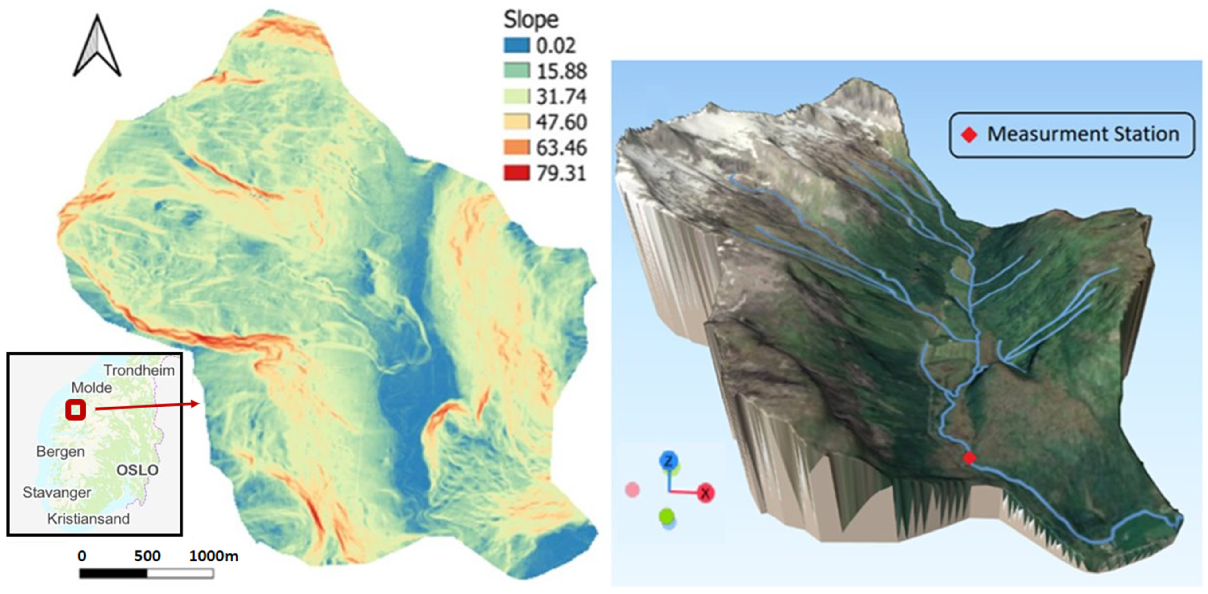
A small and steep catchment, Sleddalen, in Møre og Romsdal county in western Norway, was selected for this study (Figure 1). The catchment is 10.5 km2, with altitudes ranging from 77 to 1379 masl and an average slope of 0.5 m/m. Half of the catchment is covered by bare rock and scarce vegetation, while the other half is mainly covered by forest and open land. The catchment has snow-covered mountains for most of the year except for a few weeks in late summer. Digital terrain model (DTM) with a spatial resolution of 0.5 m × 0.5 m was downloaded from the Norwegian mapping authority database (hoydedata.no).
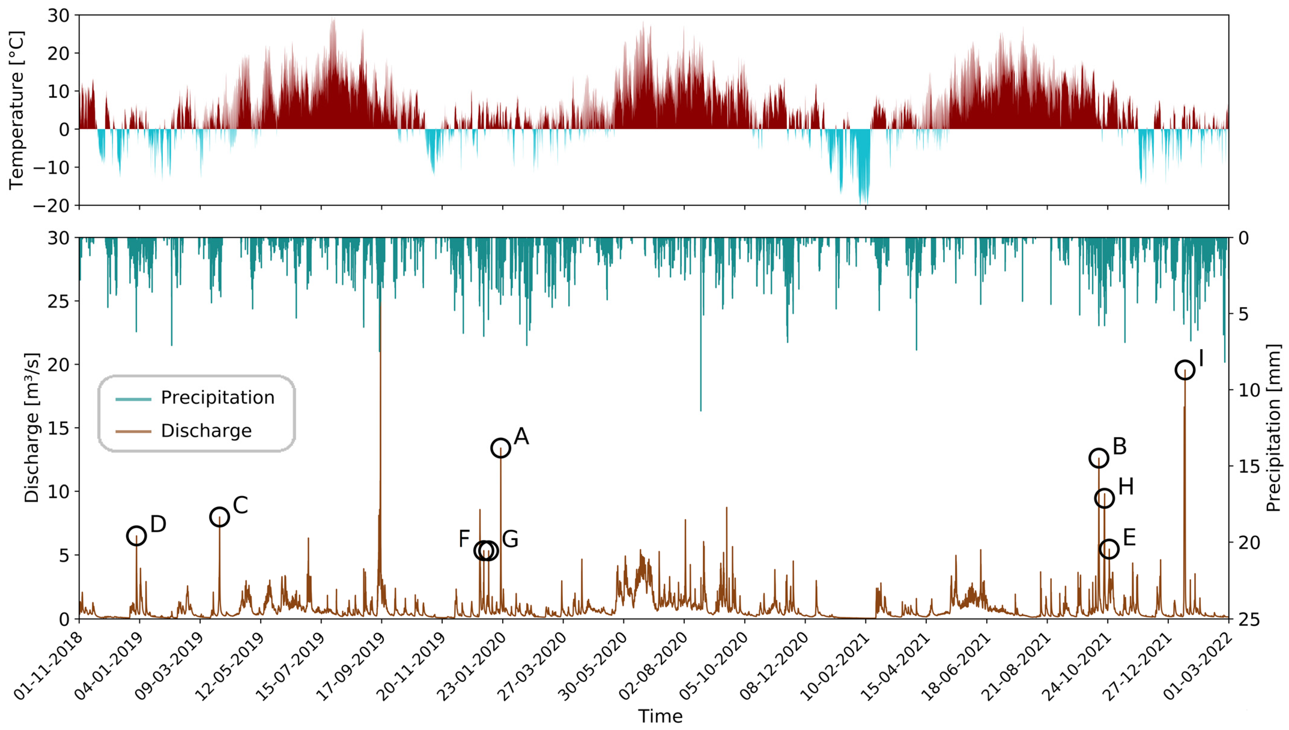
Seven peak flow events (A to G in Figure 2) from 2018 to 2022, all caused by rainfall with RoS events, were selected for the current study. Distributed precipitation data with 1 km × 1 km spatial and 1 hour temporal resolution was extracted for the catchment from the RadPro dataset from the Norwegian meteorological departments (https://www.met.no/en/projects/radpro, last accessed on 20 October 2023). RadPro is a merged product of gridded point observations and radar precipitation data [37]. Measured discharge data with 15 min temporal resolution and air temperature data with hourly resolution were downloaded for the Sleddalen measurement station (ID: 97.5.0) from Norwegian Water Resources and Energy Directorate (NVE) database available at ‘sildre.nve.no’ (Figure 2).
2.2. Methods and the Combination of Snow Routine with Integrated Hydrologic–Hydraulic Model
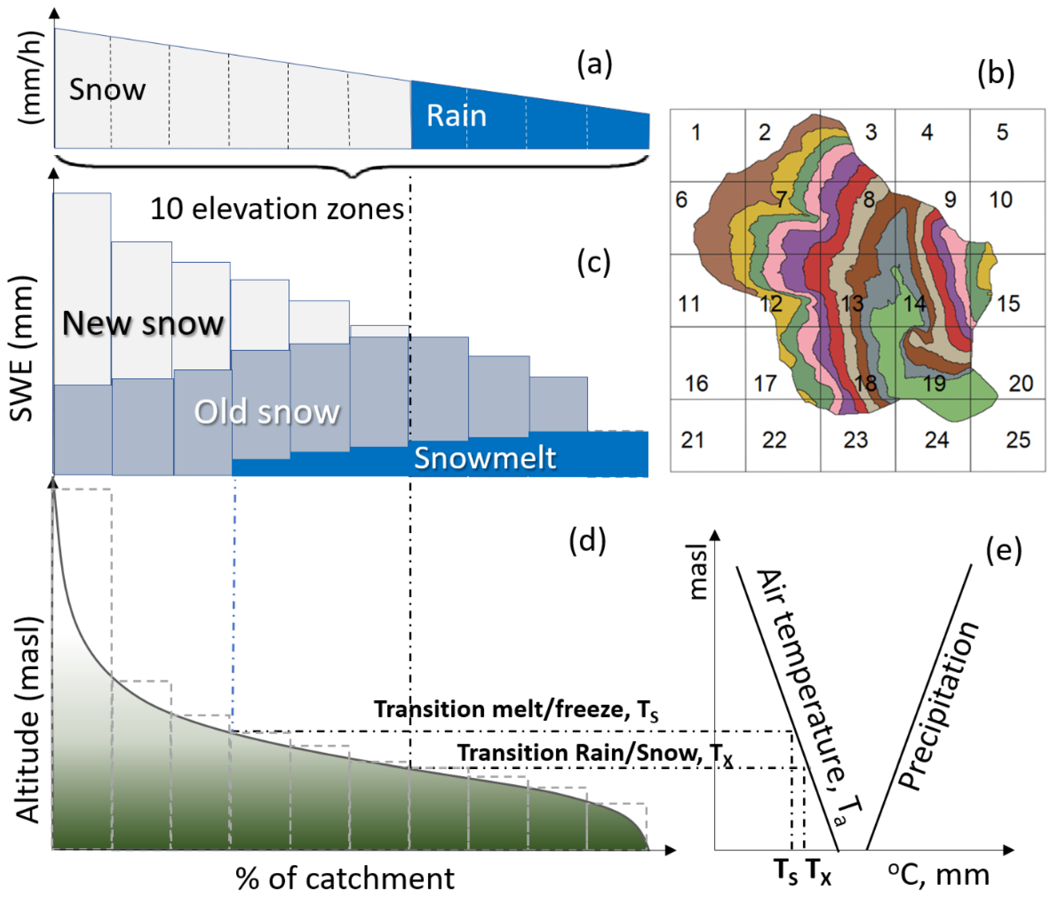
In a catchment with high altitude ranges, precipitation can occur both as rain and snow in the same timestep at different altitudes, but the snowfall does not contribute to runoff before the snow melts. The Radpro precipitation dataset does not distinguish between rain and snow. Therefore, we used HBV snow routine [35] to compute the snowmelt. The snow routine (Figure 3) calculates precipitation type and the snowmelt based on the precipitation and temperature dataset. The HBV model divides the catchment into ten equally sized elevation zones and calculates air temperature and amount and type of precipitation in each zone depending on the temperature gradients, precipitation gradients, and the threshold temperature (Tx) for snowfall [38]. The model keeps track of the accumulated snow storage in each of the elevation zones and calculates snowmelt (Equation (1)) when the temperature at the respective elevation bands is higher than the threshold for snowmelt (Ts). The snowmelt is calculated with an intensity depending on the degree day factor (Cx) and air temperature (Ta) above a snowmelt threshold temperature.
where M is the snowmelt given in mm/h, Cx is the degree day factor in mm/h °C, Ta is the air temperature in °C, and Ts is the threshold temperature for snowmelt in °C. Parameters Tx and Cx are calibrated for each event. The observed temperature and precipitation are adjusted to each elevation zone according to the lapse rate for temperature (dry or wet adiabatic) and precipitation (Figure 3e). Snowfall occurs at temperatures below a snowfall threshold temperature (Figure 3a,e). Lapse rates, threshold temperatures, and the degree-day factor are calibrated to fit discharge from simulated snowmelt events to observed and simulated snow storage to actual snow storage (exhausted at the end of summer). The snow routine also accounts for accumulation of liquid water in the snow and, thus, the delayed rain and snowmelt–water output from the snowpack [39].
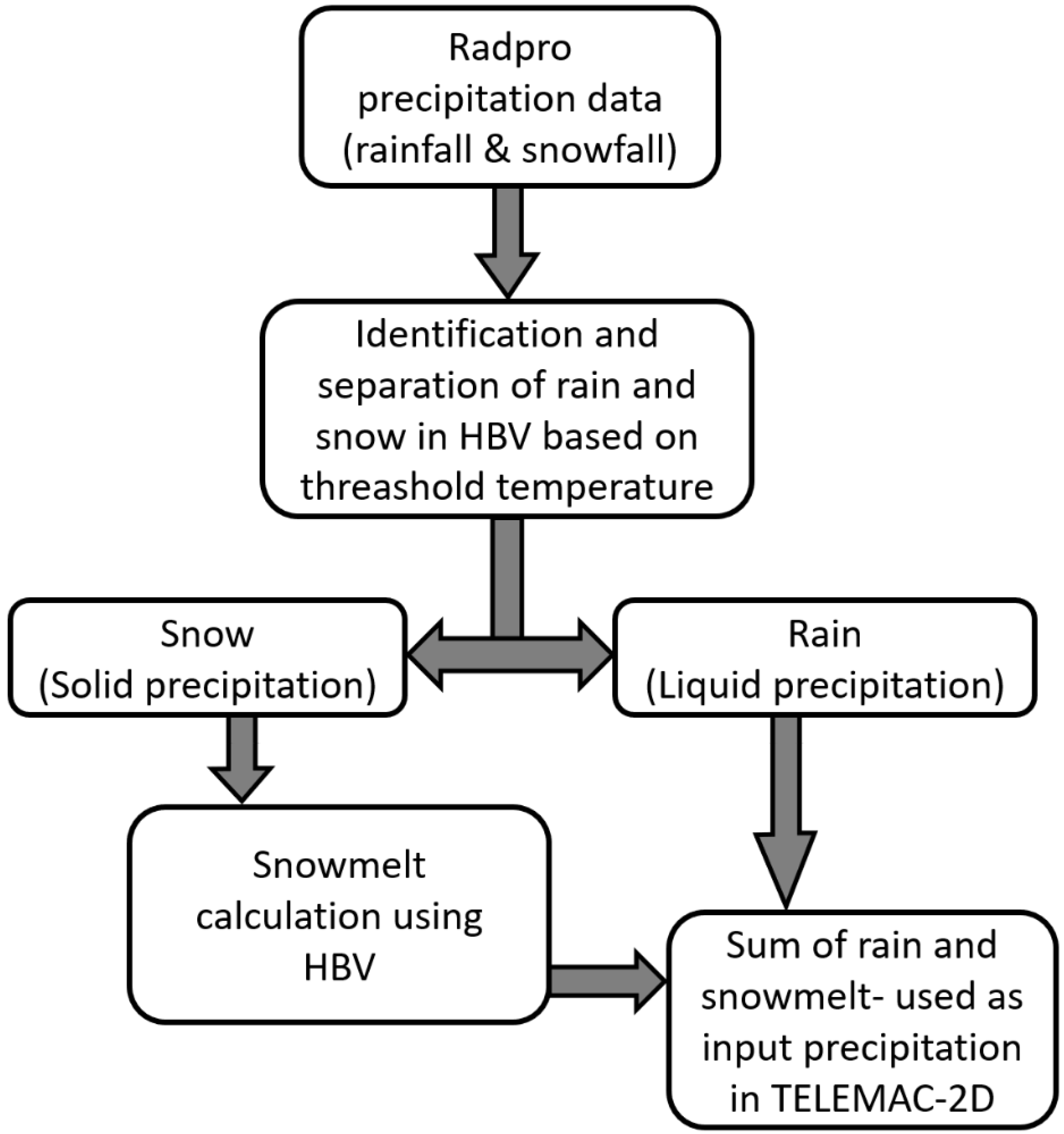
The model was run on hourly resolution with precipitation calculated to the elevation zone from the 1 km × 1 km spatially distributed RadPro precipitation data (Figure 3b) and locally observed temperature data from the Sleddalen station. The HBV model was calibrated for a three-year period (2018–2021) to evaluate the overall performance, but since the purpose of this study was to evaluate the effect of snow melt in a RoG model, a calibration was also performed for each of the specific events used in this case to obtain the snowmelt as precise as possible. Better calibration of the snow routine in HBV ensures the correct precipitation input to the HDRRM. The snowmelt values and the liquid precipitation for each timestep and elevation zone were extracted from the HBV snow routine and averaged into each grid cell in the HDRRM module of TELEMAC-2D model [36]. The flow chart for this methodology is shown below in Figure 4.
TELEMAC-2D is used as an integrated hydrological–hydraulic model (aka HDRRM) in this study. It is originally a hydrodynamic model that focuses on two-dimensional depth-averaged free surface water flows and relies on the Saint Venant equation. This software (v8p2) is designed to simulate free-surface dynamics within a two-dimensional horizontal spatial framework. At each node or point within the computational grid, T2D computes parameters such as water depth and two velocity components. A finite element mesh is incorporated to enhance the precision in representing details like rivers, embankments, and roads. Additionally, there is a parallel version available, enabling the model to operate efficiently on multi-processor computers. The model’s calculation sub-routines are scripted in Fortran-90 and Python. Users have the flexibility to customize the code to suit their specific needs. The source code of T2D model is customized in this study to use spatially distributed precipitation as input from a previous study [40]. The main inputs required are DTM, roughness values, and boundary conditions such as water flow or water surface elevation. The code in T2D model simultaneously solves the following hydrodynamic equations:
- (a)
- Continuity equation:
- (b)
- Momentum equation along x:
- (c)
- Momentum equation along y:
(m) = water depth;
, (m/s) = velocity components;
(m/s2) = gravity acceleration;
(m2/s) = momentum coefficient;
(m) = free surface elevation;
(s) = time;
, (m) = horizontal space coordinates;
(m/s) = source or sink of fluid;
, , and are the unknowns.
The model also has a supplement to include a spatially distributed rainfall-runoff module making it a hydrodynamic rainfall–runoff model (HDRRM) [41]. The curve number (CN) method is used for infiltration modelling in TELEMAC-2D. This method was developed by the USDA Natural Resources Conservation Services (NRCS) in 1950s [42] for predicting direct runoff. CN is a dimensionless empirical parameter based on the land use, soil cover, and antecedent moisture and hydrological conditions in the catchment. The following equation is used to calculate the direct runoff depth:
where Q is the direct runoff depth in mm, P is the event precipitation depth in mm, λ is the initial abstraction ratio in percentage, S in mm is the potential maximum retention, and Ia in mm is initial abstraction used as 20% of the potential maximum retention in the current study.
Based on findings from a previous study by Godara et al. [40] using TELEMAC-2D on the same catchment, parameters such as the antecedent moisture conditions (AMC), roughness, and mesh size were kept constant, and the model was calibrated only for CN values. The calibration results from that study showed that courser the mesh size, drier the catchment, and higher the roughness, the lower the runoff volume and vice versa. Since the CN value is a calibration parameter here, these values change for each event and are, therefore, different from the calibrated values for another set of events in the previous study by Godara et al. [40]. As most of the catchment is covered by forests, open land, bare rock, and scarce vegetation, spatially distributed CN values were calibrated manually only for these land covers (marked green in Table 1) whereas same CN values are used for the other land-covers (marked yellow in Table 1) for the seven peak flow events (events A to G in Figure 2).
Manning’s roughness values were calculated based on land use data from the Geonorge map catalogue, which were calibrated in a previous study for the same catchment [40] and used directly in this study.
AMC can be classified into three categories based on soil moisture levels: dry (I), normal (II), and wet (III). As there was no information available on the moisture level of the soil prior to the events, and since the CN values were not adjusted for the different moisture conditions in the catchment, we used AMC values corresponding to normal moisture conditions in this study. In addition, a correction of CN for the steep slope was applied for all these simulations. The base flow for each event was set based on the measured discharge. A 5 m by 5 m triangular mesh was used for the river and surrounding areas, while a 100 m by 100 m mesh was used for the rest of the catchment. The input file preparation such as roughness, rainfall, mesh generation, CN values over the mesh, and the post-processing of TELEMAC-2D results were carried out using python, QGIS (3.16), and Blukenue (3.3.4) software [43].
3. Results
3.1. HBV
The overall calibration of the HBV model for the period September 2018 to September 2021 gave a Nash–Sutcliffe efficiency (NSE) of 0.70, whereas for the specific events (A to I) used in this study, the NSE values were 0.94, 0.94, 0.91, 0.71, 0.86, 0.93, 0.62, 0.95, and 0.96, respectively for HBV simulations.
3.2. TELEMAC-2D
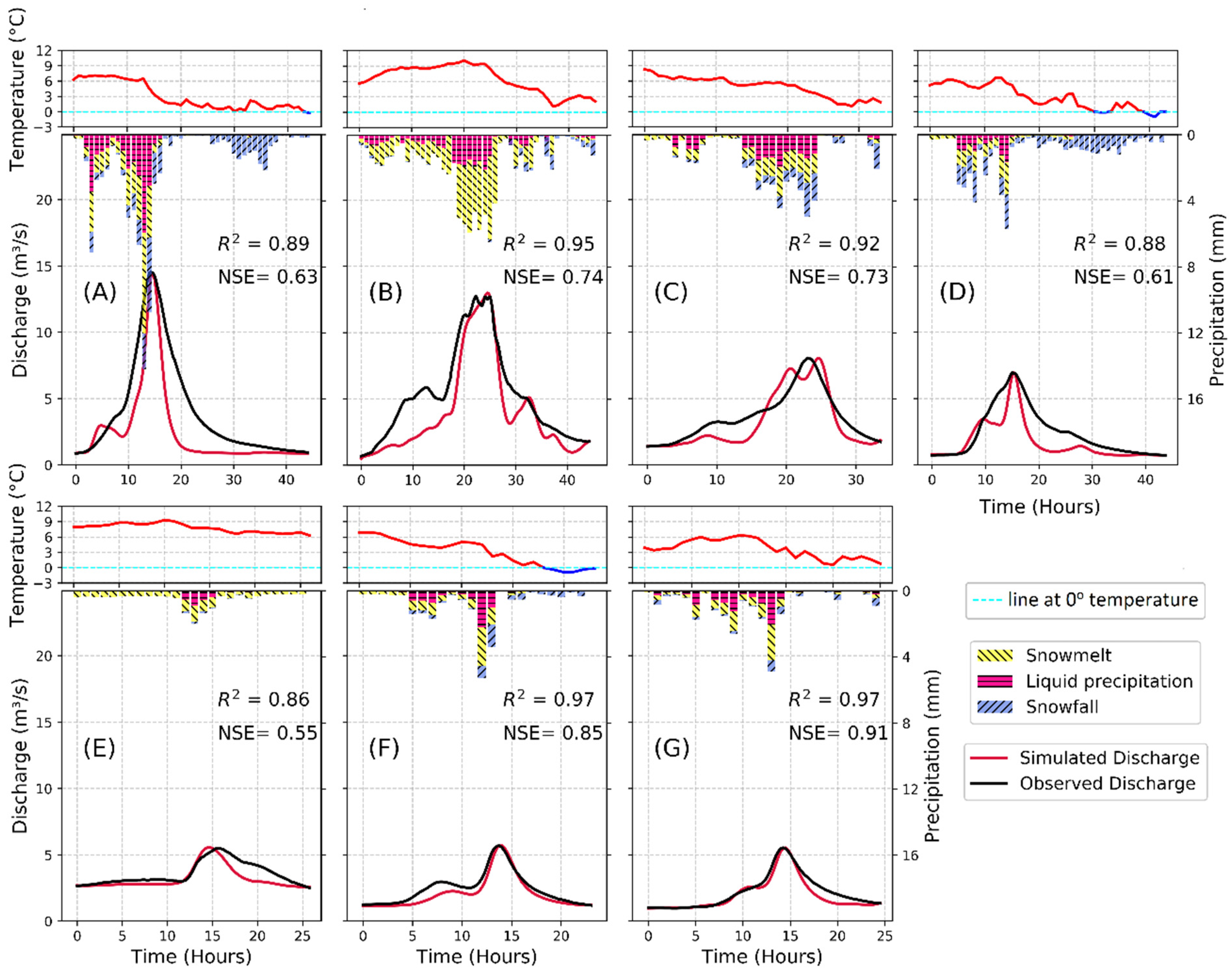
The results from TELEMAC-2D simulations corresponding to the seven peak flow events (A to G) produced via combined liquid precipitation and snowmelt are shown in Figure 5. The solid precipitation (snow), which does not contribute to the runoff during the event, is also shown in the same figure. Nash–Sutcliffe efficiency (NSE) for these events ranged from 0.55 to 0.91, and Pearson correlation coefficient (R2) values ranged from 0.86 to 0.97, as shown in Figure 5.
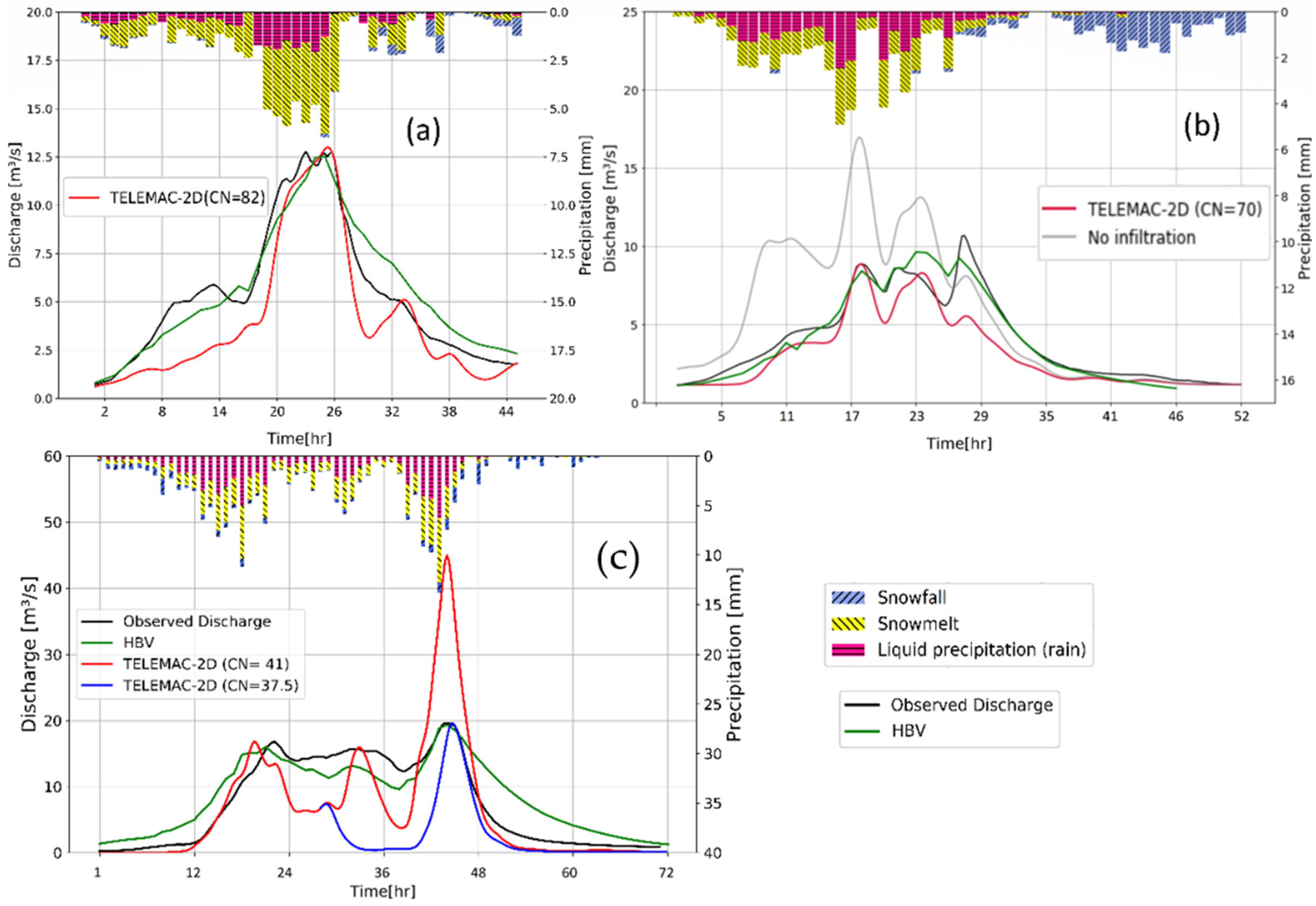
Figure 6a compares the results from a case-specific calibrated HBV model and TELEMAC-2D for the same event, as shown in Figure 5B. The HBV model accurately simulates the event with an NSE of 0.94, but TELEMAC-2D is not able to reproduce the first part of the flood as accurately with an NSE of 0.74. However, both models perform well in capturing the magnitude and timing of the peak flow. For the events in Figure 6, the catchment was calibrated with a single averaged value of CN (CNavg) to test if it gives equally satisfactory results if no soil data are available for catchment [40].
In Figure 6c, the first simulation is run with a CNavg of 41. It captured the first peak but overestimated the second peak since the CN 41 becomes too high as the catchment grows more saturated. So, to capture the second peak, another simulation was run with a lower CN value using the output from the first simulation as the initial condition (known as a hotstart file) keeping all the other parameters the same.
Figure 6b,c show that the HBV model can simulate rain-on-snow events with longer durations and multiple peaks (NSE > 0.95), while TELEMAC-2D is not able to capture the entire events. In Figure 6b, the hydrograph from TELEMAC with a CN value of 100 (grey) represents the flow without infiltration, while the hydrograph with a CNavg of 70 satisfactorily reproduces the first peak but fails to capture the last. In Figure 6c, a CNavg of 41 in TELEMAC-2D accurately simulates the first peak, but a higher average infiltration rate is needed to simulate the last peak (CNavg = 37.5). However, it was not possible to accurately simulate the high sustained discharge throughout the event, regardless of the choice of curve number.
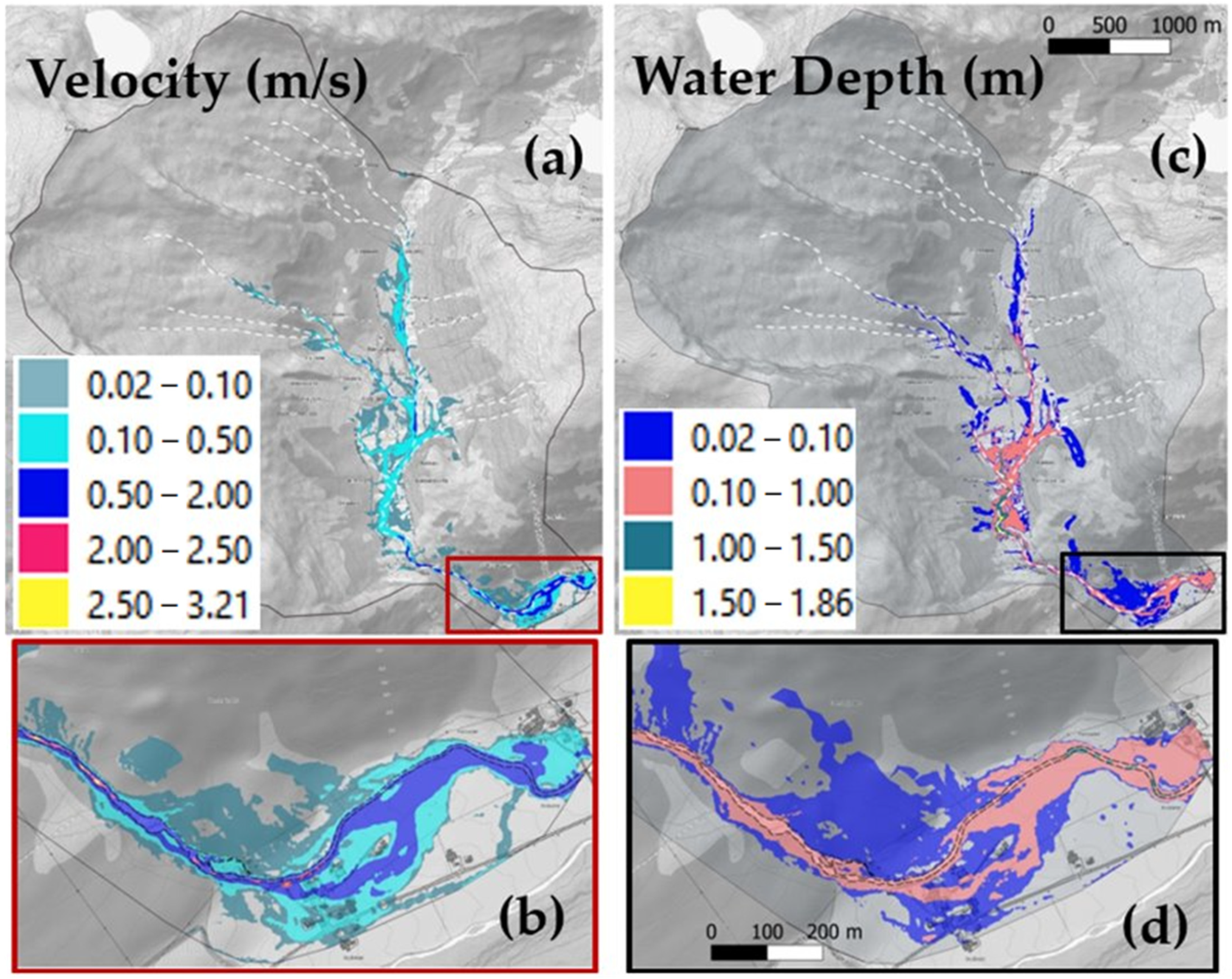
Figure 7 shows the maximum water depth and velocity results in the entire catchment for the event shown in Figure 5A with a peak discharge of 14.55 m3/s from RoG HDRRM modelling. The figure also shows that the river network generated via the model is similar to the digitized river network from the Norwegian Water Administration database in Figure 7a. Maximum water velocities are 3.21 m/s, which may cause erosion, leading to serious sedimentation problems in the lower regions where the water depths are up to 1.86 m. The figure shows also that even with a 100 by 100 m grid cell size, the RoG model captures the river network and flow paths quite well compared to the digitized river network from the Norwegian Water Administration database.
4. Discussion
This study analyses flash flood events caused by RoS events in small and steep snow-covered mountainous catchments using the RoG version of TELEMAC-2D combined with snowmelt calculation from the HBV model. The resulting RoG simulations for the investigated events indicate that the approach used in this study satisfactorily reproduces single peak flows, the inflow sources, and tributaries. However, as the hydraulic model is not calibrated towards observed water depths due to a lack of such information, the simulated water velocities and water depth are only indicative. Flood data from past flood events should be used for calibration and verifying the application of this technique in future studies. Nevertheless, the results of the current study provide crucial information for flood protection at any point along the river system in the catchment (Figure 7). High water levels and velocity locations are identified using the current technique, which is important information for contingency planners. Critical locations and risk levels in the catchment can be determined using the product of water depths and water velocity in terms of pedestrian, vehicle, and building safety [44,45,46].
An NSE of 0.70 for the period from 2018 to 2022 indicates that the HBV model is also able to reproduce the floods for Sleddalen. An average NSE for the seven events of 0.84 in HBV compared to 0.71 for the RoG in TELEMAC-2D shows that the HBV model demonstrates a more accurate reproduction of the flood events in this study. However, the HBV model does not provide information on velocities, flooded areas, and water depths and is, therefore, not a sufficient tool for flood mitigation or preparedness. This is, nevertheless, an indication of a better hydrological approach in the HBV model than in the RoG TELEMAC-2D.
The good fit between the observed runoff and HBV-simulated runoff for the selected events shows that the calculated snowmelt for these events is a reliable input to the RoG model. In addition, the results, when combined with the rain from the RadPro data, show that the RadPro data represent true precipitation satisfactorily. The RoG model worked well for single peak events, whereas it did not give satisfactory results in the case of longer flood events with multiple peaks. In complex mountainous areas such as in western Norway, it is difficult to capture the correct spatial distribution of the precipitation either by gauge stations, radar datasets, or high-resolution interpolated data sets because the pattern is strongly influenced by the complex terrain [47]. Hence, the model results are subject to uncertainty due to the input data. However, the good fit achieved via the HBV model indicates that the input is probably not the cause of the poor simulation via RoG in TELEMAC-2D for events lasting over longer periods. It is also important to mention that the results from the hydrologic and hydraulic models are subjected to various uncertainties in the models themselves [48] and in the input data such as precipitation, digital elevation model, bathymetry of the river, and roughness [49].
The calibration results of TELEMAC-2D for CN values show decreasing CN values and thus a higher infiltration as the rainfall depth increases, which is a contradiction to an expected higher saturation and less infiltration during longer events [50]. However, this finding is coherent with the results from the study by Krvavica and Rubinić [51]. A possible explanation for this is that since RoG TELEMAC-2D does not simulate the subsurface drainage of infiltrated water, which, in nature, comes back to the river system, TELEMAC-2D compensates by a higher surface runoff using low infiltration capacity (high CN). For a longer duration flood, a low infiltration (high CN) gives a good fit in the initial stage but gives too high discharge at later stages. Vice versa, a high infiltration rate used to fit the model to a later peak in a longer flood event gives too low discharge in the early stage. This can explain why the first small peak in Figure 6a is not correctly reproduced via TELEMAC-2D, but the later peak flows are well captured via the TELEMAC-2D as well as HBV. Since the HBV model includes soil storage and runoff from infiltrated water, it performs better for longer events and events with multiple rain peaks as the case in the event in Figure 6b,c. For the same reasons, it better handles the increase in the discharge in situations with saturated conditions prior to the event and also the recession part of the flow as illustrated in the event in Figure 6a. However, in contrast to the HBV model, TELEMAC-2D with RoG technique gives the hydraulic conditions, such as water levels, velocities, and inundated areas along the watercourses in the catchment. As TELEMAC-2D, in contradiction to the HBV model, does not include water storages, the infiltered water will not return and contribute as subsurface drainage to the base flow in a later stage of the flood. Another consequence of this, which is apparent in all the cases, is a steeper recession limb compared to the observed.
Similarly, in Figure 6b, TELEMAC-2D is not able to maintain a high discharge during the entire event because even after the catchment is completely saturated, the continuing abstractions kept occurring based on the CN value selected. A solution to this can be a time-varying CN value in a single simulation, as illustrated in Figure 6c. A simulation with an average CN value of 41, which captured the first peak, was combined with a simulation with a lower CN to capture the last peak. Here, only two CN values were used, but this indicates that a continuous transition of curve numbers from high to low during the event can possibly enable RoG TELEMAC-2D to reconstruct the longer, multi-peaked floods. The CN value is used as a calibration parameter in this study, and the results are sensitive to the CN values in determining the runoff volume [40]. Each flood event from the same catchment needs to be calibrated against a CN value. Therefore, further investigation is necessary to better understand the factors influencing CN values and to develop a methodology for selecting an appropriate CN value for specific storm events. A sensitivity analysis in the previous study [40] has shown that CN values and antecedent moisture conditions (AMCs) in the catchment are very crucial factors that influence the output runoff volume. Nevertheless, the analysis did not reveal any distinct correlation between CN and cumulative rainfall over the preceding five days, base flow, or the flow peak. Since CN is a calibration parameter in this study, the proposed integrated HDRRM model cannot be used as a forecasting model but can be used satisfactorily for the identification and post-analysis of the consequences of flood events. In order to employ this approach as a predictive model, the variability of the CN values among various events needs to be further investigated. The varying CN value is an issue here, and further work is needed to understand why CN value varies for each event. However, the multiple CN values calibrated for each flood event can be utilized to conduct an ensemble analysis of outputs for predictive analysis.
Since the CN method is a lumped conceptual approach that was originally developed for single storm events [52], the results for the sustained flow events align with what could be expected. However, it is important to examine the consequences of such events. A solution to satisfactorily simulate multi-peak flood events can either be to include variable CN values in RoG T2D or implement another hydrological model allowing for storage and subsurface drainage back to the river system as in the HBV model. Such a combination can also be used to integrate the snowmelt and rain with hydraulic simulations in rain-on-grid models as demonstrated in this study.
5. Conclusions
The main objective of this study was to examine the effects of the snowmelt contribution in flash flood events and to see how snowmelt calculations can be combined with the rain-on-grid method in an HDRRM model. Since a snowmelt routine is not available in the HDRRM T2D model, an external snowmelt algorithm from the HBV model was used and integrated with the rain-on-grid technique in the TELEMAC-2D model. This study’s purpose and objectives have been successfully fulfilled as evidenced by generated flood maps and depth and velocity maps. Significantly, this study demonstrated that these analyses could be executed without using the conventional methodology of using a separate hydrological model for discharge computation, followed by its use as input in a hydraulic routing model. The implementation of a soil and snow storage routine in the RoG hydraulic models would give a valuable contribution to flash flood mitigation and contingency work because such a combination gives both the hydrology and the hydraulics in the river and catchment in a continuous operational simulation model.
Author Contributions
Conceptualization, N.G., O.B. and K.A.; methodology, N.G., O.B. and K.A.; software, N.G.; validation, N.G.; formal analysis, N.G.; investigation: N.G. and resources, N.G., O.B. and K.A.; data curation, N.G.; writing—original draft preparation, N.G.; writing—review and editing, N.G. and O.B.; visualization, N.G. and O.B.; supervision, O.B. and K.A.; project administration, O.B.; funding acquisition, O.B. All authors have read and agreed to the published version of the manuscript.
Funding
This publication is part of the World of Wild Waters (WoWW) project number 949203100, which falls under the umbrella of the Norwegian University of Science and Technology (NTNU)’s Digital Transformation initiative.
Data Availability Statement
The data that support the findings of this study are available from the corresponding author, N.G., upon reasonable request.
Conflicts of Interest
The authors declare no conflict of interest. The funders had no role in the design of this study; in the collection, analyses, or interpretation of data; in the writing of the manuscript, or in the decision to publish the results.
References
- Sweeney, T.L. Modernized Areal Flash Flood Guidance. NOAA Technical Memorandum NWS HYDRO. 1992. Available online: https://repository.library.noaa.gov/view/noaa/13498 (accessed on 20 October 2023).
- Zhang, Y.; Wang, Y.; Chen, Y.; Xu, Y.; Zhang, G.; Lin, Q.; Luo, R. Projection of changes in flash flood occurrence under climate change at tourist attractions. J. Hydrol. 2021, 595, 126039. [Google Scholar] [CrossRef]
- Zhang, Y.; Wang, Y.; Chen, Y.; Liang, F.; Liu, H. Assessment of future flash flood inundations in coastal regions under climate change scenarios—A case study of Hadahe River basin in northeastern China. Sci. Total Environ. 2019, 693, 133550. [Google Scholar] [CrossRef] [PubMed]
- Modrick, T.M.; Georgakakos, K.P. The character and causes of flash flood occurrence changes in mountainous small basins of Southern California under projected climatic change. J. Hydrol. Reg. Stud. 2015, 3, 312–336. [Google Scholar] [CrossRef]
- Swanston, D.N. Slope Stability Problems Associated with Timber Harvesting in Mountainous Regions of the Western United States; Pacific Northwest Research Station, US Department of Agriculture, Forest Service: Washington, DC, USA, 1974. [Google Scholar]
- Johnson, J.P.L.; Whipple, K.X.; Sklar, L.S. Contrasting bedrock incision rates from snowmelt and flash floods in the Henry Mountains, Utah. Geol. Soc. Am. Bull. 2010, 122, 1600–1615. [Google Scholar] [CrossRef]
- Sandersen, F.; Bakkehøi, S.; Hestnes, E.; Lied, K. The influence of meteorological factors on the initiation of debris flows, rockfalls, rockslides and rockmass stability. Publ.-Nor. Geotek. Inst. 1997, 201, 97–114. [Google Scholar]
- Heyerdahl, H.; Høydal, Ø.A. Geomorphology and Susceptibility to Rainfall Triggered Landslides in Gudbrandsdalen Valley, Norway. Adv. Cult. Living Landslides 2017, 4, 267–279. [Google Scholar] [CrossRef]
- Pall, P.; Tallaksen, L.M.; Stordal, F. A climatology of rain-on-snow events for Norway. J. Clim. 2019, 32, 6995–7016. [Google Scholar] [CrossRef]
- Hansen, B.B.; Isaksen, K.; Benestad, R.E.; Kohler, J.; Pedersen, Å.Ø.; Loe, L.E.; Coulson, S.J.; Larsen, J.O.; Varpe, Ø. Warmer and wetter winters: Characteristics and implications of an extreme weather event in the High Arctic. Environ. Res. Lett. 2014, 9, 114021. [Google Scholar] [CrossRef]
- Krug, A.; Primo, C.; Fischer, S.; Schumann, A.; Ahrens, B. On the temporal variability of widespread rain-on-snow floods. Meteorol. Z. 2020, 29, 147–163. [Google Scholar] [CrossRef]
- Schmocker-Fackel, P.; Naef, F. Changes in flood frequencies in Switzerland since 1500. Hydrol. Earth Syst. Sci. 2010, 14, 1581–1594. [Google Scholar] [CrossRef]
- Sui, J.; Koehler, G. Rain-on-snow induced flood events in southern Germany. J. Hydrol. 2001, 252, 205–220. [Google Scholar] [CrossRef]
- Uhlemann, S.; Thieken, A.H.; Merz, B. A consistent set of trans-basin floods in Germany between 1952–2002. Hydrol. Earth Syst. Sci. 2010, 14, 1277–1295. [Google Scholar] [CrossRef]
- Gvoždíková, B.; Müller, M. Evaluation of extensive floods in western/central Europe. Hydrol. Earth Syst. Sci. 2017, 21, 3715–3725. [Google Scholar] [CrossRef]
- Musselman, K.N.; Lehner, F.; Ikeda, K.; Clark, M.P.; Prein, A.F.; Liu, C.; Barlage, M.; Rasmussen, R. Projected increases and shifts in rain-on-snow flood risk over western North America. Nat. Clim. Chang. 2018, 8, 808–812. [Google Scholar] [CrossRef]
- Marks, D.; Kimball, J.; Tingey, D.; Link, T. The sensitivity of snowmelt processes to climate conditions and forest cover during rain-on-snow: A case study of the 1996 Pacific Northwest flood. Hydrol. Process. 1998, 12, 1569–1587. [Google Scholar] [CrossRef]
- McCabe, G.J.; Clark, M.P.; Hay, L.E. Rain-on-snow events in the western United States. Bull. Am. Meteorol. Soc. 2007, 88, 319–328. [Google Scholar] [CrossRef]
- Pomeroy, J.W.; Fang, X.; Marks, D.G. The cold rain-on-snow event of June 2013 in the Canadian Rockies—Characteristics and diagnosis. Hydrol. Process. 2016, 30, 2899–2914. [Google Scholar] [CrossRef]
- Kattelmann, R. Flooding from rain-on-snow events in the Sierra Nevada. IAHS-AISH Publ. 1997, 239, 59–65. [Google Scholar]
- Seneviratne, S.I.; Zhang, X.; Adnan, M.; Badi, W.; Dereczynski, C.; Di Luca, A.; Ghosh, S.; Iskandar, I.; Kossin, J.; Ewitson, B.; et al. IPCC—Climate Change 2021: The Physical Science Basis; Chapter 11: Weather and Climate Extreme Events in a Changing Climate; Cambridge University Press: Cambridge, UK; New York, NY, USA, 2021; p. 1610. [Google Scholar] [CrossRef]
- Førland, E.J.; Skaugen, T.E.; Benestad, R.E.; Hanssen-Bauer, I.; Tveito, O.E. Variations in thermal growing, heating, and freezing indices in the Nordic Arctic, 1900–2050. Arct. Antarct. Alp. Res. 2004, 36, 347–356. [Google Scholar] [CrossRef]
- Rantanen, M.; Karpechko, A.Y.; Lipponen, A.; Nordling, K.; Hyvärinen, O.; Ruosteenoja, K.; Vihma, T.; Laaksonen, A. The Arctic has warmed nearly four times faster than the globe since 1979. Commun. Earth Environ. 2022, 3, 168. [Google Scholar] [CrossRef]
- Singh, P.; Spitzbart, G.; Hübl, H.; Weinmeister, H. Hydrological response of snowpack under rain-on-snow events: A field study. J. Hydrol. 1997, 202, 1–20. [Google Scholar] [CrossRef]
- Sati, V.P. Glacier bursts-triggered debris flow and flash flood in Rishi and Dhauli Ganga valleys: A study on its causes and consequences. Nat. Hazards Res. 2022, 2, 33–40. [Google Scholar] [CrossRef]
- Roald, L.A. Floods in Norway. In Changes in Flood Risk in Europe; CRC Press: Boca Raton, FL, USA, 2019. [Google Scholar]
- Yang, Z.; Yuan, X.; Liu, C.; Nie, R.; Liu, T.; Dai, X.; Ma, L.; Tang, M.; Xu, Y.; Lu, H. Meta-Analysis and Visualization of the Literature on Early Identification of Flash Floods. Remote Sens. 2022, 14, 3313. [Google Scholar] [CrossRef]
- Merz, R.; Blöschl, G. A process typology of regional floods. Water Resour. Res. 2003, 39, 1340. [Google Scholar] [CrossRef]
- Surfleet, C.G.; Tullos, D. Variability in effect of climate change on rain-on-snow peak flow events in a temperate climate. J. Hydrol. 2013, 479, 24–34. [Google Scholar] [CrossRef]
- Blöschl, G.; Bierkens, M.F.P.; Chambel, A.; Cudennec, C.; Destouni, G.; Fiori, A.; Kirchner, J.W.; McDonnell, J.J.; Savenije, H.H.G.; Sivapalan, M.; et al. Twenty-three unsolved problems in hydrology (UPH)–a community perspective. Hydrol. Sci. J. 2019, 64, 1141–1158. [Google Scholar] [CrossRef]
- Li, D.; Lettenmaier, D.P.; Margulis, S.A.; Andreadis, K. The Role of Rain-on-Snow in Flooding Over the Conterminous United States. Water Resour. Res. 2019, 55, 8492–8513. [Google Scholar] [CrossRef]
- Costabile, P.; Costanzo, C.; Ferraro, D.; Barca, P. Is HEC-RAS 2D accurate enough for storm-event hazard assessment? Lessons learnt from a benchmarking study based on rain-on-grid modelling. J. Hydrol. 2021, 603, 126962. [Google Scholar] [CrossRef]
- David, A.; Schmalz, B. A systematic analysis of the interaction between rain-on-grid-simulations and spatial resolution in 2d hydrodynamic modeling. Water 2021, 13, 2346. [Google Scholar] [CrossRef]
- Norwegian Directorate for Civil Protection (DSB). Analyses of Crisis Scenarios 2019; DSB Skien: Porsgrunn, Norway, 2019; pp. 1–228. Available online: https://www.dsb.no/rapporter-og-evalueringer/analyses-of-crisis-scenarios-2019/ (accessed on 20 October 2023).
- Bergström, S.; Forsman, A. Development of a conceptual deterministic rainfall-runoff model. Nord. Hydrol. 1973, 4, 240–253. [Google Scholar] [CrossRef]
- Ligier, P. Implementation of a rainfall-runoff model in TELEMAC-2D. In Proceedings of the XXIIIrd TELEMAC-MASCARET User Conference 2016, Paris, France, 11–13 October 2016. [Google Scholar]
- Engeland, K.; Abdella, S.Y.; Azad, R.; Arrturi Elo, C.; Lussana, C.; Tadege Mengistu, Z.; Nipen, T.; Randriamampianina, R. Use of precipitation radar for improving estimates and forecasts of precipitation estimates and streamflow. In Proceedings of the 20th EGU General Assembly, EGU2018, Vienna, Austria, 4–13 April 2018; 2018; p. 12207. [Google Scholar]
- Killingtveit, A.; Sælthun, N.R. Hydropower Development: Hydrology; NTNU: Trondheim, Norge, 1995. [Google Scholar]
- Bruland, O. Snow processes, modeling, and impact. In Precipitation; Elsevier Inc.: Amsterdam, The Netherlands, 2021; pp. 107–143. [Google Scholar] [CrossRef]
- Godara, N.; Bruland, O.; Alfredsen, K. Simulation of flash flood peaks in a small and steep catchment using rain-on-grid technique. J. Flood Risk Manag. 2023, 16, e12898. [Google Scholar] [CrossRef]
- Broich, K.; Pflugbeil, T.; Disse, M.; Nguyen, H. Using TELEMAC-2D for Hydrodynamic Modeling of Rainfall-Runoff. In Proceedings of the 26th TELEMAC-MASCARET User Conference, Toulouse, France, 15–17 October 2019. [Google Scholar]
- The ASCE/EWRI Curve Number Hydrology Task Committee. Curve Number Hydrology; Hawkins, R.H., Ward, T.J., Woodward, D.E., Van Mullem, J.A., Eds.; American Society of Civil Engineers: Reston, VA, USA, 2008; ISBN 9780784410042. [Google Scholar]
- Barton, A.J. Blue Kenue Enhancements from 2014 to 2019. In Proceedings of the 26th TELEMAC-MASCARET User Conference, Toulouse, France, 15–17 October 2019. [Google Scholar] [CrossRef]
- Shand, T.; Smith, G.; Cox, R.; Blacka, M. Development of Appropriate Criteria for the Safety and Stability of Persons and Vehicles in Floods. In Proceedings of the 34th World Congress of the International Association for Hydro—Environment Research and Engineering: 33rd Hydrology and Water Resources Symposium and 10th Conference on Hydraulics in Water Engineering, Brisbane, Australia, 26 June–1 July 2011; p. 9. [Google Scholar]
- Direktoratet for Byggkvalitet. Veiledning om Tekniske Krav Til Byggverk; TEK17. 2017. Available online: http://www.jurpc.de/jurpc/show?id=20140073 (accessed on 20 September 2023).
- Skrede, T.I.; Muthanna, T.M.; Alfredesen, K. Applicability of urban streets as temporary open floodways. Hydrol. Res. 2020, 51, 621–634. [Google Scholar] [CrossRef]
- Li, L.; Pontoppidan, M.; Sobolowski, S.; Senatore, A. The impact of initial conditions on convection-permitting simulations of a flood event over complex mountainous terrain. Hydrol. Earth Syst. Sci. 2020, 24, 771–791. [Google Scholar] [CrossRef]
- McMillan, H.K.; Westerberg, I.K.; Krueger, T. Hydrological data uncertainty and its implications. WIREs Water 2018, 5, e1319. [Google Scholar] [CrossRef]
- Annis, A.; Nardi, F.; Volpi, E.; Fiori, A. Quantifying the relative impact of hydrological and hydraulic modelling parameterizations on uncertainty of inundation maps. Hydrol. Sci. J. 2020, 65, 507–523. [Google Scholar] [CrossRef]
- Hjelmfelt, A.T. Investigation of Curve Number Procedure. J. Hydraul. Eng. 1991, 117, 725–737. [Google Scholar] [CrossRef]
- Krvavica, N.; Rubinić, J. Evaluation of design storms and critical rainfall durations for flood prediction in partially urbanized catchments. Water 2020, 12, 2044. [Google Scholar] [CrossRef]
- USDA-SCS. Part 630 Hydrology National Engineering Handbook. Chapter 10 Estimation of Direct Runoff from Storm Rainfall. 2004. Available online: https://directives.sc.egov.usda.gov/OpenNonWebContent.aspx?content=17752.wba (accessed on 20 October 2023).
Figure 1.
Location of the study area in Norway along with the catchment slope in degrees (left) and a picture showing the steepness, vegetation cover and the discharge and temperature measurement stations in the area (right).
Figure 1.
Location of the study area in Norway along with the catchment slope in degrees (left) and a picture showing the steepness, vegetation cover and the discharge and temperature measurement stations in the area (right).

Figure 2.
Time series with hourly temporal resolution from November 2018 to March 2022 showing observed discharge, precipitation, temperature, the seven single peak events (A to G), and two longer flood events with multiple peaks (H and I) selected for this study.
Figure 2.
Time series with hourly temporal resolution from November 2018 to March 2022 showing observed discharge, precipitation, temperature, the seven single peak events (A to G), and two longer flood events with multiple peaks (H and I) selected for this study.

Figure 3.
Snow routine in the HBV model with (a) hourly precipitation input in the form of rain and snow defined by (e) the temperature and precipitation gradients, threshold values and intensities from (b) the RadPro grid cells (also showing the elevation zones), (c) resulting accumulated new and old snow and snowmelt, (d) Hypsographic curve of the catchment with the ten elevation zones.

Figure 4.
Flow chart for the methodology used.

Figure 5.
Simulated discharge from TELEMAC-2D, observed discharge, liquid (rain) and solid (snow) precipitation and snowmelt, temperature (upper) corresponding to the seven single peak events (A–G) selected for this study.
Figure 5.
Simulated discharge from TELEMAC-2D, observed discharge, liquid (rain) and solid (snow) precipitation and snowmelt, temperature (upper) corresponding to the seven single peak events (A–G) selected for this study.

Figure 6.
(a) Simulated discharge from TELEMAC-2D (red) and from HBV (green) calibrated for a single peak event B in Figure 2. (b) Simulated flow from TELEMAC-2D for CN = 70 (red) (R2 = 0.93) and for CN = 100 (no infiltration) (grey) corresponding to the multi-peak event H in Figure 2. (c) Single simulation in TELEMAC-2D for entire event with CN = 41 (red), another TELEMAC-2D simulation with CN = 37.5 (blue) for 2nd peak, and the result from calibrated HBV only (R2 = 0.87) (green) corresponding to the multi-peak event I in Figure 2.

Figure 7.
(a) Digitized river network from Norwegian Water Administration database (white dotted river lines) and flow velocity in the entire catchment. (b) Velocities in populated areas (red rectangle). (c) Water depths in entire catchment and (d) in the populated area (black rectangle) for the event shown in Figure 5A.


Table 1.
Calibrated CN values corresponding to the seven events A to G (in Figure 2) along with their date and time of occurrence.
Table 1.
Calibrated CN values corresponding to the seven events A to G (in Figure 2) along with their date and time of occurrence.
| Description | Area (%) | Event A [20 January 2020 (10:00)-44 hours] | Event B [13 October 2021 (16:00)-45 hours] | Event C [28 March 2019 (17:00)-33 hours] | Event D [31 December 2018 (04:00)-44 hours] | Event E [24 January 2020 (23:00)-25 hours] | Event F [2 January 2020 (12.00)-23 hours] | Event G [7 January 2020 (14:00)-24 hours] |
|---|---|---|---|---|---|---|---|---|
| Bare rock and scarce vegetation | 46.57 | 50 | 84 | 64 | 72 | 80 | 72 | 74 |
| Forest | 25.05 | 45 | 73 | 61 | 68 | 74 | 68 | 71 |
| Open land | 20.00 | 43 | 70 | 59 | 65 | 72 | 65 | 69 |
| Swamp | 3.62 | 90 | ||||||
| Fully cultivated soil | 3.24 | 90 | ||||||
| Inland pasture | 0.86 | 89 | ||||||
| River water | 0.38 | 100 | ||||||
| Urban Area | 0.19 | 89 | ||||||
| Roads | 0.10 | 91 | ||||||
Disclaimer/Publisher’s Note: The statements, opinions and data contained in all publications are solely those of the individual author(s) and contributor(s) and not of MDPI and/or the editor(s). MDPI and/or the editor(s) disclaim responsibility for any injury to people or property resulting from any ideas, methods, instructions or products referred to in the content. |
© 2023 by the authors. Licensee MDPI, Basel, Switzerland. This article is an open access article distributed under the terms and conditions of the Creative Commons Attribution (CC BY) license (https://creativecommons.org/licenses/by/4.0/).
Share and Cite
MDPI and ACS Style
Godara, N.; Bruland, O.; Alfredsen, K. Modelling Flash Floods Driven by Rain-on-Snow Events Using Rain-on-Grid Technique in the Hydrodynamic Model TELEMAC-2D. Water 2023, 15, 3945. https://doi.org/10.3390/w15223945
AMA Style
Godara N, Bruland O, Alfredsen K. Modelling Flash Floods Driven by Rain-on-Snow Events Using Rain-on-Grid Technique in the Hydrodynamic Model TELEMAC-2D. Water. 2023; 15(22):3945. https://doi.org/10.3390/w15223945
Chicago/Turabian StyleGodara, Nitesh, Oddbjørn Bruland, and Knut Alfredsen. 2023. "Modelling Flash Floods Driven by Rain-on-Snow Events Using Rain-on-Grid Technique in the Hydrodynamic Model TELEMAC-2D" Water 15, no. 22: 3945. https://doi.org/10.3390/w15223945
Note that from the first issue of 2016, this journal uses article numbers instead of page numbers. See further details here.