


Comparative Assessment of Different Image Velocimetry Techniques for Measuring River Velocities Using Unmanned Aerial Vehicle Imagery

1
Department of Civil and Disaster Prevention Engineering, National United University, Miaoli 360302, Taiwan
2
Department of Civil Engineering, Diponegoro University, Semarang 50275, Indonesia
*
Author to whom correspondence should be addressed.
Water 2023, 15(22), 3941; https://doi.org/10.3390/w15223941
Submission received: 30 September 2023
/
Revised: 4 November 2023
/
Accepted: 8 November 2023
/
Published: 12 November 2023
(This article belongs to the Special Issue Advances in Hydrology: Flow and Velocity Analysis in Rivers)
Abstract
:The accurate measurement of river velocity is essential due to its multifaceted significance. In response to this demand, remote measurement techniques have emerged, including large-scale particle image velocimetry (LSPIV), which can be implemented through cameras or unmanned aerial vehicles (UAVs). This study conducted water surface velocity measurements in the Xihu River, situated in Miaoli County, Taiwan. These measurements were subjected to analysis using five distinct algorithms (PIVlab, Fudaa-LSPIV, OpenPIV, KLT-IV, and STIV) and were compared with surface velocity radar (SVR) results. In the quest for identifying the optimal parameter configuration, it was found that an IA size of 32 pixels × 32 pixels, an image acquisition frequency of 12 frames per second (fps), and a pixel size of 20.5 mm/pixel consistently yielded the lowest values for mean error (ME) and root mean squared error (RMSE) in the performance of Fudaa-LSPIV. Among these algorithms, Fudaa-LSPIV consistently demonstrated the lowest mean error (ME) and root mean squared error (RMSE) values. Additionally, it exhibited the highest coefficient of determination (R2 = 0.8053). Subsequent investigations employing Fudaa-LSPIV delved into the impact of various water surface velocity calculation parameters. These experiments revealed that alterations in the size of the interrogation area (IA), image acquisition frequency, and pixel size significantly influenced water surface velocity. This parameter set was subsequently employed in an experiment exploring the incorporation of artificial particles in image velocimetry analysis. The results indicated that the introduction of artificial particles had a discernible impact on the calculation of surface water velocity. Inclusion of these artificial particles enhanced the capability of Fudaa-LSPIV to detect patterns on the water surface.
1. Introduction
River flow velocity plays a crucial role in water resource management and river flood prevention, necessitating constant measurements regardless of flood or drought seasons [1]. However, obtaining accurate observations in river areas, particularly during floods, remains challenging and limited [2]. Conventional methods for measuring surface flow velocities, such as acoustic Doppler current profilers and current meters, require expensive equipment and manpower during measurements [1,3]. Moreover, obtaining surface velocities from an ADCP might also be difficult due to blanking distance and post-processing might be needed. To address this issue, there has been a growing interest in utilizing recorded videos or image velocimetry to measure flow velocities [1].
Originally, image velocimetry utilized cameras to monitor river flow and evolved into a non-contact technique for natural channels known as large-scale particle image velocimetry (LSPIV), capable of monitoring river flow with various applications and generating two-dimensional (2D) flow fields [4]. LSPIV provides detailed information about velocity vector angles and magnitudes, capturing the spatial variability along the river from the video data [5,6]. In engineering demonstrations, LSPIV has shown promising results, with an error value of 10% when compared to micro-propeller ADCP and numerical simulations [7]. Additionally, LSPIV measurements exhibit good agreement with ADCP velocities, with a deviation of ±10% [8]. Studies in Sweden (with a lack of natural particles) and Denmark (with artificial particles) reported a velocity error of 10 cm/s and an R-squared value (R2) greater than 0.7, indicating the effectiveness of LSPIV [6]. Moreover, LSPIV has been used as a benchmark for the validation and calibration of 2D hydraulic models, showing comparable results to traditional ADCP measurements [9].
The potential of LSPIV has led to the development of diverse software tools to calculate surface flow velocity [10]. Each software employs different analysis techniques, making it essential to compare their accuracy (see Table 1). Commonly used software includes particle image velocimetry (PIV) tools such as PIVlab [11], OpenPIV [12], and Fudaa-LSPIV [13,14]. Additionally, other algorithms like Kanade Lucas Tomasi (KLT) are utilized, with KLT-IV [15] being one of the notable tools, as well as space time image velocimetry (STIV) [16,17,18,19,20] represented by RIVeR-STIV (Table 1).
Image velocimetry has been widely employed in the field using either handheld cameras or cameras mounted onto buildings overlooking the water surface. However, with the advancements in technology, a growing number of studies have utilized unmanned aerial vehicles (UAVs) to capture images and videos of river bodies. In hydrology, UAVs have proven advantageous due to their ability to gather data in hazardous environments and conduct large-scale observations, making them an ideal tool for surface flow observation [21,22,23,24]. Furthermore, UAV-based data gathering has proven to be more cost-effective and efficient compared to traditional remote sensing methods for surface flow observation [25,26,27]. The agility of UAVs allows for swift operations and comprehensive coverage of the entire river body, capturing wide views from vantage points that are unattainable from the ground [4,28]. Given these advantages, the use of video data obtained through UAVs reduces the necessity for extensive image correction and transformation. As a result, potential errors are minimized, and the time required for operational analysis is significantly reduced [4,29]. This reduction in potential errors maximizes the analytical potential of image velocimetry for accurately assessing water surface velocity.
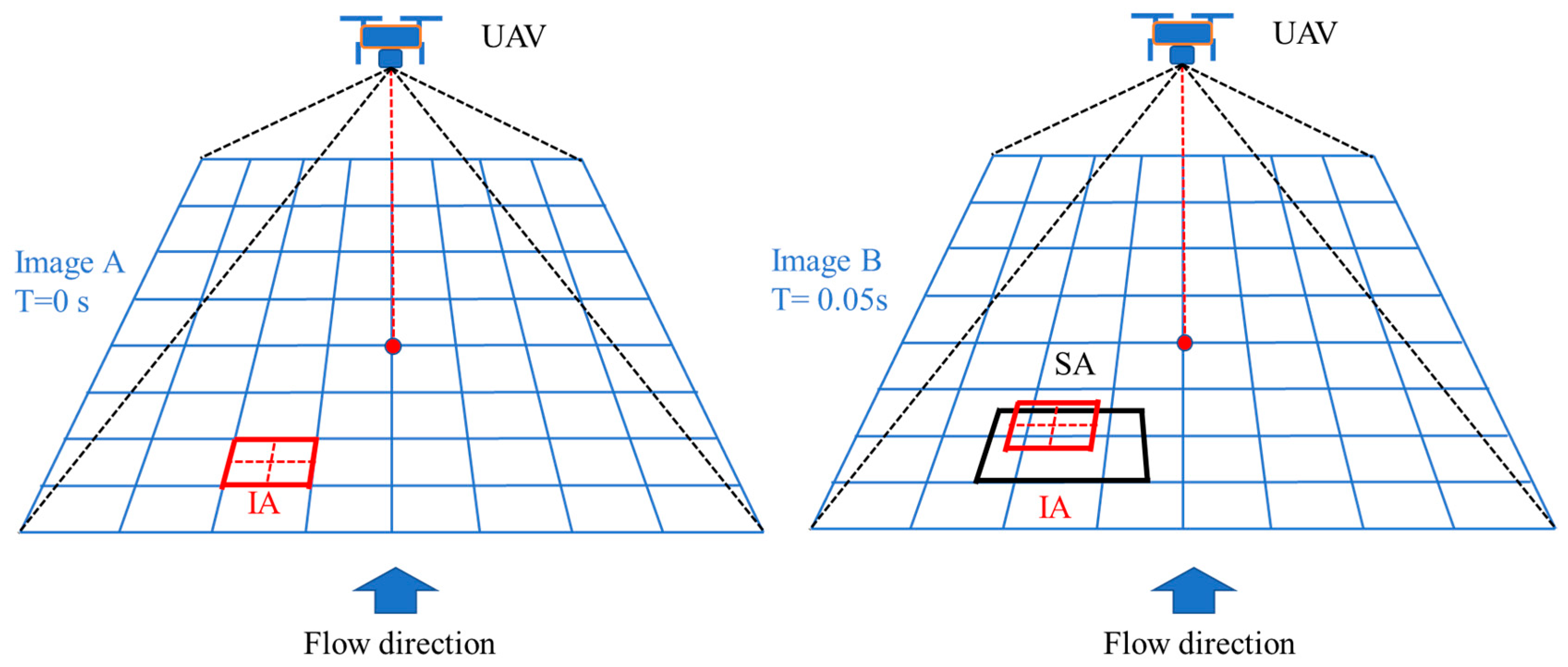
In image velocimetry software, an essential aspect is the presence of particles or patterns on the river surface, which are utilized to calculate surface flow velocities [30]. The method relies on the displacement of particles groups or image textures. The resulting flow velocities are determined on a regular grid known as the surface velocity field (SVF). Each cell on this grid, called the interrogation area (IA), is used to determine the most probable particles displacements [29]. Figure 1 illustrates the relationship between IA (represented by the red box) and SA (depicted by the black box). The IA in the second image searches within the SA to find the position with the highest similarity to the IA in the first image. Calculating the flow velocity is achievable by dividing the distance between the IA in the two images by the time difference between them.
Aside from the IA and SA, other factors like the image frequency or frame rate from videos or images also influence velocity analysis results. Particles displacement is calculated using the formula , where V is the velocity in meters per second (m/s), is the distance between two images of IA, and is the time difference between two images. Image frequency is adjusted accordingly to suit particles displacement, especially when there is minimal displacement between frames [4]. The height from which a river image or video is captured impacts image visibility. Flying height and camera characteristics dictate the pixel size. Higher UAV flights result in increased ground distance, represented by one pixel in the image [2]. All of these parameters are interrelated and can be improved through parameter optimization to obtain better parameter values [31].
To improve the image processing and velocity calculation, artificial particles may need to be added to the river. These artificial particles or seeds assist LSPIV in detecting patterns on the water’s surface, making it easier to infer its velocities. The accuracy of LSPIV depends on critical factors like the size, shape, and color of these artificial particles. The density of particles seeding also influences LSPIV’s effectiveness in detecting movement patterns. Moreover, artificial color and contrast enhance the success of image processing, particularly when there is a lack of light, which could otherwise reduce pattern identification [30].
The main purpose of this study is to examine methodologies and techniques employed by common software tools, namely PIVlab, Fudaa-LSPIV, OpenPIV, KLT-IV, and RIVeR-STIV. Additionally, this investigation delves into the pivotal factors that contribute to the precision of water surface velocity computations, including the IA, SA, artificial tracer, pixel size, and video frame rate. The acquisition of data videos and frames was carried out using a UAV. Subsequently, the obtained results were subjected to a comparative analysis against the surface velocity radar (SVR) to establish a benchmark. Gaining insights into the advantages and constraints of each software tool, as well as comprehending the influential factors, will enhance the user’s proficiency in analyzing water surface velocity. Such knowledge empowers researchers to make informed decisions and optimally utilize these tools to analyze the surface velocity of water.
2. Materials and Methods
2.1. Image Velocimetry Process
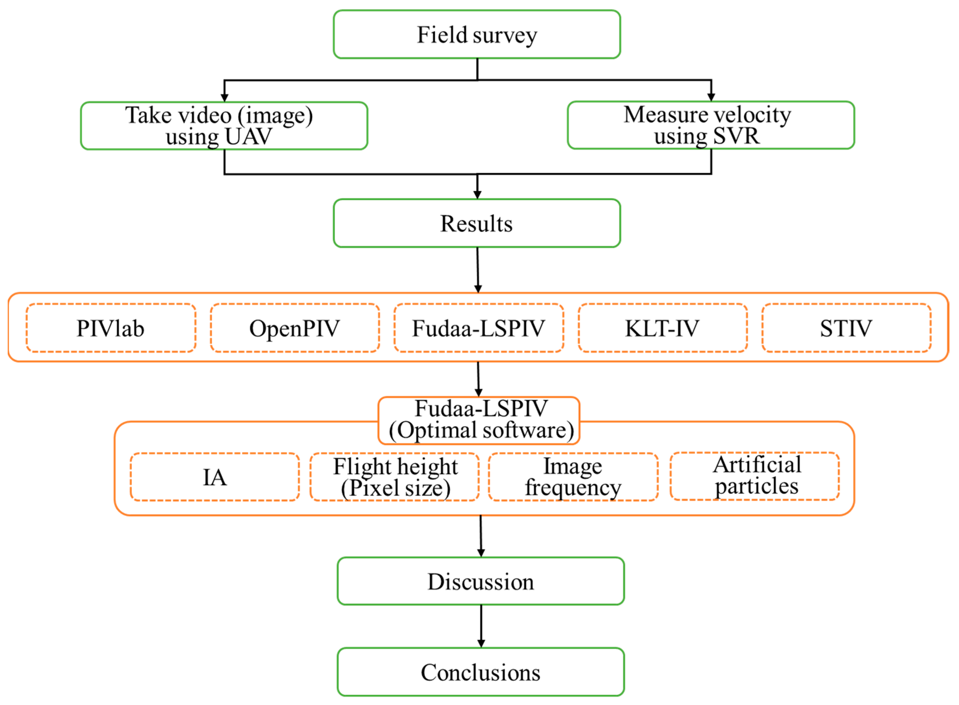
The flowchart of this study method is depicted in Figure 2. It commences with field surveys to assess river geometry and identify suitable UAV flight locations. Once the field conditions are known, data are collected through manual measurements using SVR and measurements using UAV. Subsequently, the UAV data are analyzed using five freely accessible software tools for image-based velocimetry analysis: PIVlab, Fudaa-LSPIV, OpenPIV, KLT-IV, and STIV. The objective is to determine the most suitable software for analyzing river surface velocity through a comparison of their performance under specific parameters.
In this study, an analysis of five software programs is conducted, with an emphasis on comparing their results while employing identical parameters. The optimal parameter set, determined through the examination of multiple parameter configurations, is subsequently applied to all five software programs for the purpose of comparison. Following this, the software program that exhibits the superior performance is utilized to explore the impact of various parameters on the analysis outcomes, including IA, pixel size, and image frequency. Moreover, the study delves into the influence of artificial particles on the analysis results, recognizing the significance of particles presence on water surfaces as an external factor in LSPIV. Each parameter’s individual effect on analysis outcomes is addressed separately to mitigate the potential for errors stemming from simultaneous alterations in multiple parameters. Finally, a discussion and conclusion are presented.
The results of the analysis from the five types of software are compared with the results of the SVR to determine the most suitable software for analyzing river conditions. Various parameters such as IA, image frequency, and pixel size can affect the water surface velocity analysis results, along with the presence of artificial particles. The study concludes with a discussion of the advantages and limitations of these factors and software tools.
2.2. Description of the Study Area
The research was conducted in the Xihu River, located in Xihu Township, Miaoli County. The main stream originates from the Guandao Mountain at an elevation of 889 m in Sanyi Township, while its tributary, the Shuiwei River, starts at the northern foot of Mountain Jitu at 548 m. Both streams converge on the north side of the Sanyi road, passing through Tongluo Township and Xihu Township. The total length of the river is approximately 32 km, and the river basin covers an area of about 110 km2.
The study area is situated on the Xihu River, within the provincial road section (Figure 3a). The constant flow of the river allows for easy access and conduct of studies by communities. The river’s width is influenced by the flow and water level, as the river banks contain silt and sand that can be easily washed away by water. The flow direction is shown in Figure 3b, and the river’s width ranges from 12 to 21 m, depending on environmental conditions and water level. The measured section’s width is depicted in Figure 4.
To measure the water velocity, manual measurements were performed by two individuals pulling a rope at both ends of the river to ascertain a straight line, while SVR was used to measure the water velocity every 0.5 m along the red line, as shown in Figure 3b. The variability of the number of points is dependent on the discharge, as shown in Table 2. Additionally, UAVs were used to capture river surface conditions, with videos of durations ranging from 20 to 50 s. The experiments, conducted on 23 August and 18 September, involved the release of additional particles via wood shavings (Table 2).
After analyzing the surface velocity using various LSPIV software with images captured with a UAV, it was possible to manually select the positions of personnel holding fixed tape measures from the images. Finally, along a straight line connecting the two image coordinates, surface velocities were compared at intervals of 50 cm.
2.3. Unmanned Aerial Vehicle (UAV)
In this study, the unmanned aerial vehicle employed for image and video capture along the river was the DJI Phantom 4 Pro (DJI P4P, Shenzhen Dajiang Innovation Technology Co. Ltd, Shenzhen, China, https://www.dji.com/tw/phantom-4-pro/info, accessed on 30 October 2023) series. The camera equipped on the DJI P4P is capable of capturing images and videos in 4K, FHD, and HD quality, offering both single and multiple shooting options. This UAV achieves a video frame rate of 24−30 frames per second, ensuring smooth footage. Thanks to its four-axis stabilized gimbal, this UAV maintains stable balance during image capture, effectively reducing any in-air shaking.
However, due to its compact size, the chosen UAV is susceptible to wind interference during takeoff. This study conducted flights at varying altitudes, namely 15 m, 35 m, 55 m, and 75 m, in order to make comparisons. The video size was set to 3480 pixels × 2160 pixels, so the pixel sizes corresponding to different UAV flight heights of 15 m, 35 m, 55 m, and 75 m were 7 mm/pixel, 13.8 mm/pixel, 20.5 mm/pixel, and 27.4 mm/pixel, respectively.
2.4. Surface Velocity Radar (SVR)
The study employed a handheld surface velocity radar 3D (SVR 3D, Decatur Electronics, LLC, Escondido, CA, USA, https://decaturelectronics.com/hydrology-products/svr-3d/, accessed on 30 October 2023) as its benchmark tool. SVR 3D is known for its safety and ease of use, making it highly effective for real-time water velocity measurements, especially in flood-prone situations. Obtaining results using this equipment is swift, taking just 5 s after pointing the SVR 3D towards the water surface. This device boasts spectral and spectrogram features that expedite the evaluation of water conditions. Furthermore, SVR 3D’s ergonomic design and water-resistant properties enhance its usability.
One notable advantage of SVR 3D is its automatic compensation for vertical angles, accommodating angles of up to 60° without requiring manual tilt adjustments. However, measurements should be maintained at a constant angle below 60° to ensure the accurate correction of the SVR. To maintain precision, it is essential to orient the device’s antenna parallel to the target without any horizontal (yaw) angle exceeding 10°, as exceeding this threshold can introduce measurement errors.
As per the manufacturer’s data sheet, SVR’s measurement accuracy stands at ±1% of the measured value. This impressive accuracy range extends from 0.1 m/s to 33 m/s, making SVR 3D a versatile and reliable tool for a wide range of water velocity measurements [32,33].
When using SVR as a sonic measurement instrument and holding it manually for measurements, it could potentially shake. Consequently, measurements were typically conducted for more than one minute in order to acquire an average value as the measurement result, thereby mitigating measurement errors.
2.5. Statistical Error
In order to assess the precision of each software’s analysis, it becomes imperative to determine the discrepancy by juxtaposing the software’s results with those generated with the SVR. The computation of this disparity for each software employs two key metrics: the mean error (ME) and the root mean square error (RMSE), computed as follows:
where N expresses the total number measured, Vs,i denotes the value measured with SVR, and Vo,i represents the LSPIV measurement using a different software.
3. Results
This section delves into a comparative analysis of five software applications employed for river velocity analysis. The experimental dataset utilized consisted of observations taken on 5 and 11 July 2022. In each experiment, data regarding water surface velocity were collected using both the SVR and UAV methods. SVR was utilized as a reference point, and its results were subsequently compared with those obtained from the UAV analysis. This analysis was carried out utilizing five different software tools: PIVlab, Fudaa-LSPIV, OpenPIV, KLT-IV, and STIV. The research first tested the configuration of parameters for five software tools, and selected a better set of parameters to be applied for comparison on all software.
All software applications were configured with identical parameters, namely an interrogation area size of 32 pixels × 32 pixels, a pixel size of 20.5 mm/pixel, and an image capture frequency of 12 fps. In the investigation of Fudaa-LSPIV and KLT-IV, as well as the implementation of PIVlab, OpenPIV, and STIV, the search area (SA) and step size were set at half of the IA. The primary objective of Section 3.1 and Section 3.2 is to identify the most optimal software for conducting surface velocity analysis.
3.1. Measurement Results on 5 July 2022
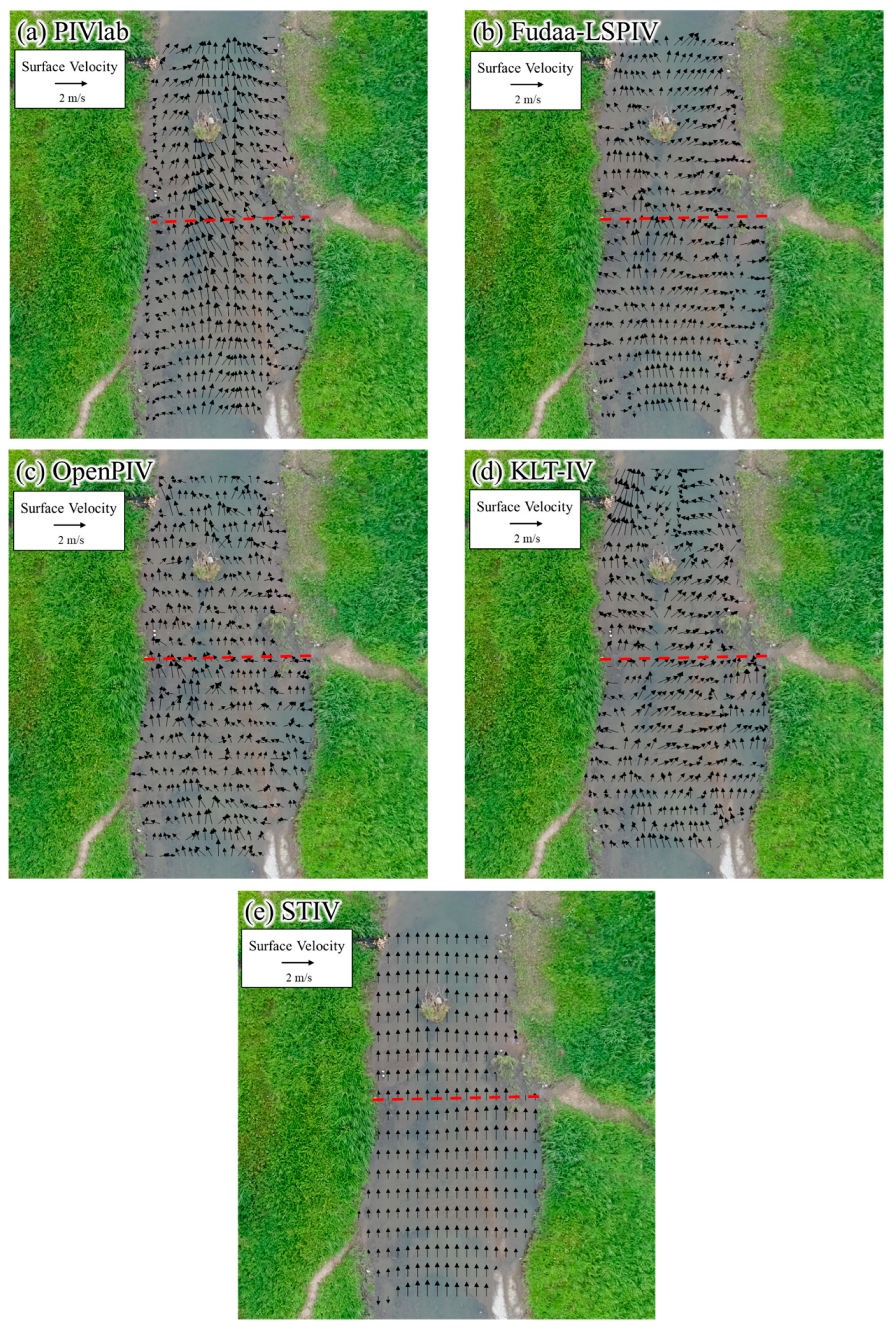
The experiment conducted on July 5th took place in challenging conditions due to the high water level in the river, making it unsafe for entry. Data collection occurred between 10 a.m. and 2 p.m., as subsequent hours were constrained by rainfall. The river’s length measures 20.5 m, and data points were recorded at 0.5 m intervals, resulting in a total of 42 data points. Video footage, lasting 24 s, was captured for analysis. Subsequently, the captured video material was subjected to analysis, and a flow field was generated in each software, as depicted in Figure 4, with the red line denoting the SVR measurement line.
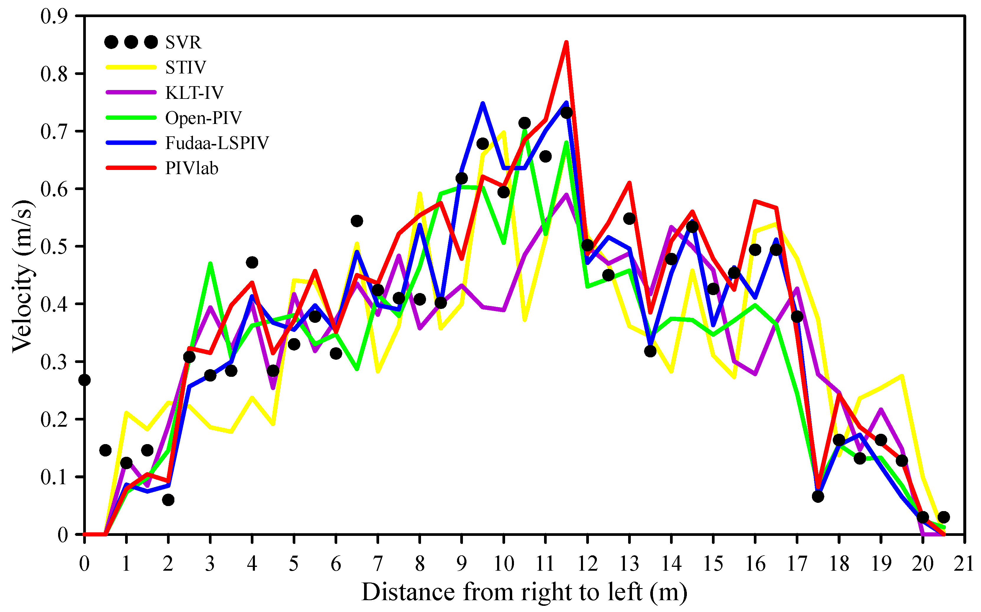
Figure 5 displays the outcomes of the image velocimetry analysis conducted on 5 July. In general, the velocities obtained with all software packages remain within reasonable limits compared to those generated via SVR. Figure 5 also reveals that all software exhibits an error within the 0−0.5 m range, with all software indicating a velocity of 0 m/s in this region. In comparing the manual measurements with the image velocimetry, the results show reasonable agreement, with water velocity increasing from the riverbank towards the middle of the river.
On the specific date of 5 July 2022, the PIV algorithm stands out for its superior ability to detect water surface movement through cross-correlation. Fudaa-LSPIV demonstrates the lowest error, with an RMSE of 0.150 m/s and ME of 0.013 m/s.
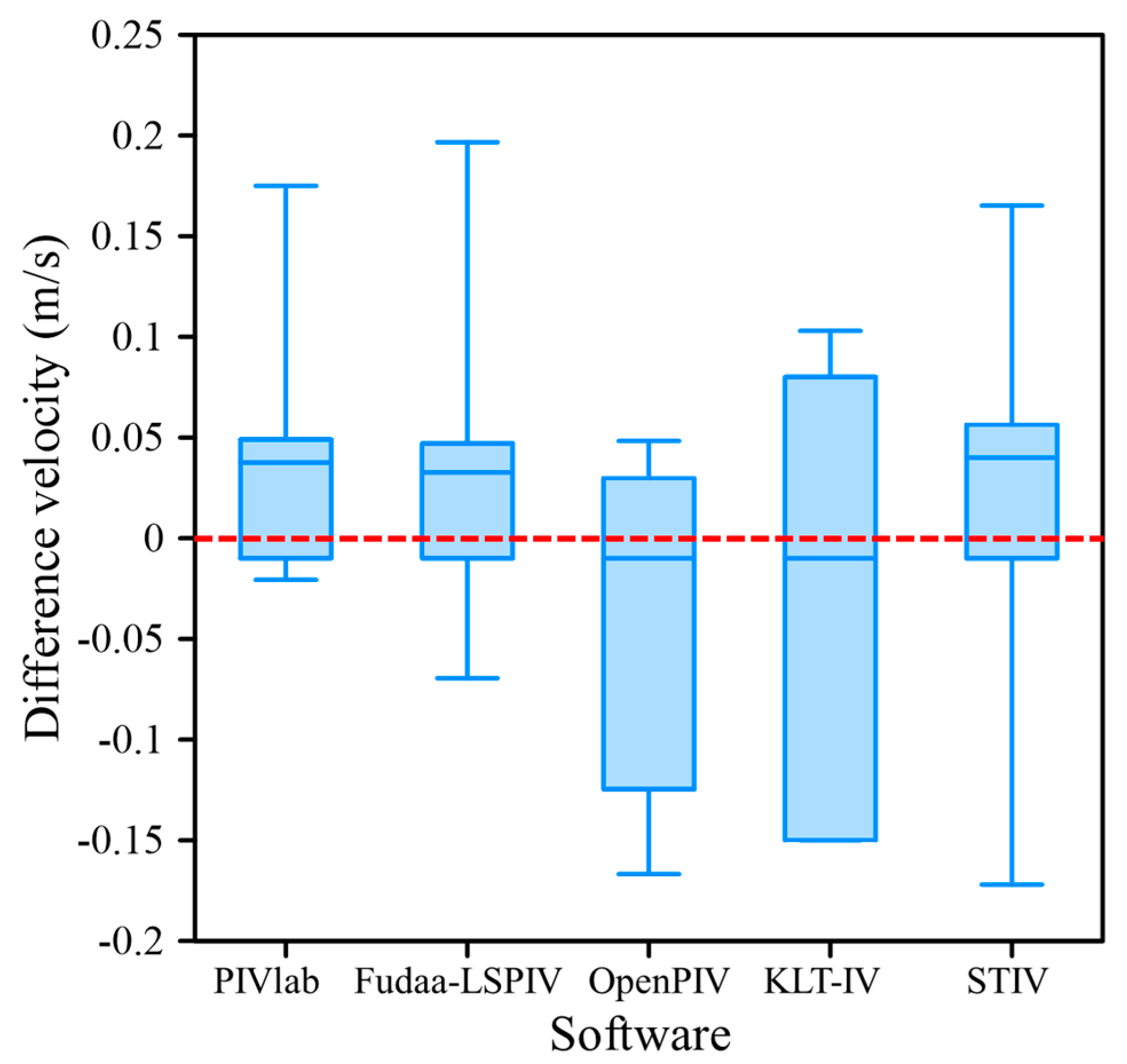
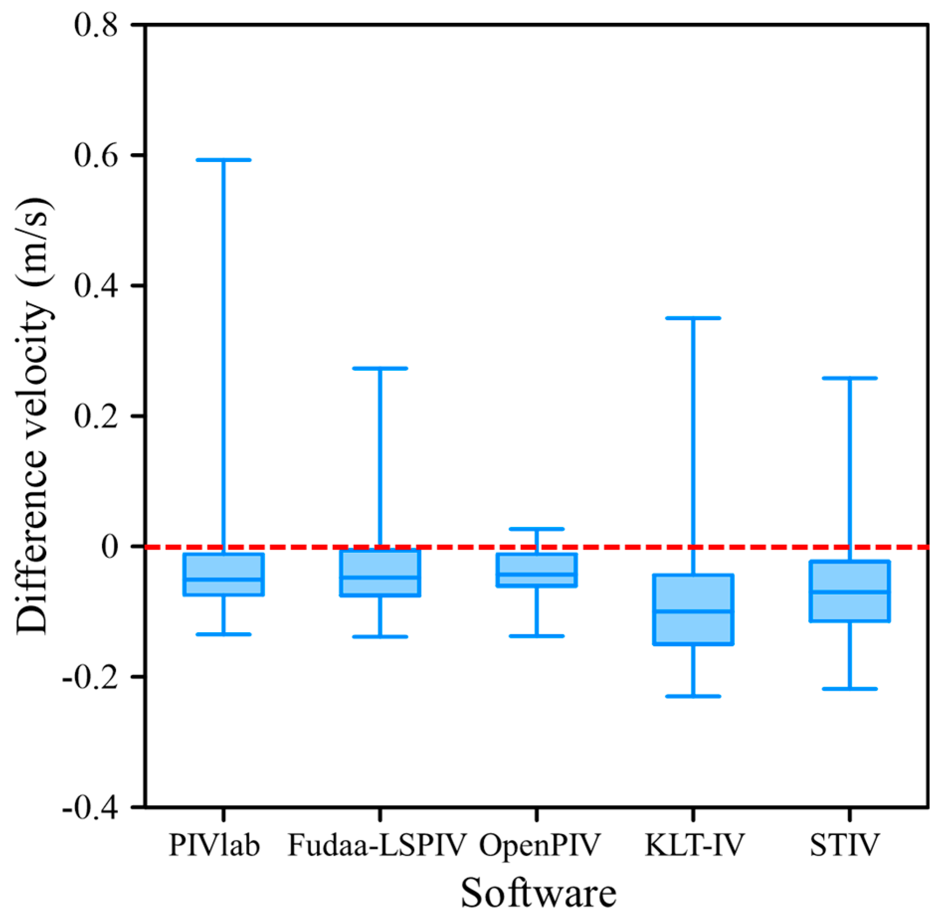
Figure 6 presents a box plot illustrating the velocity differences between the image velocimetry software and SVR. These results indicate minimal variability in the velocity difference data, with PIVlab and Fudaa-LSPIV exhibiting the same median values. However, Fudaa-LSPIV produces smaller maximum and minimum velocity values compared to PIVlab.
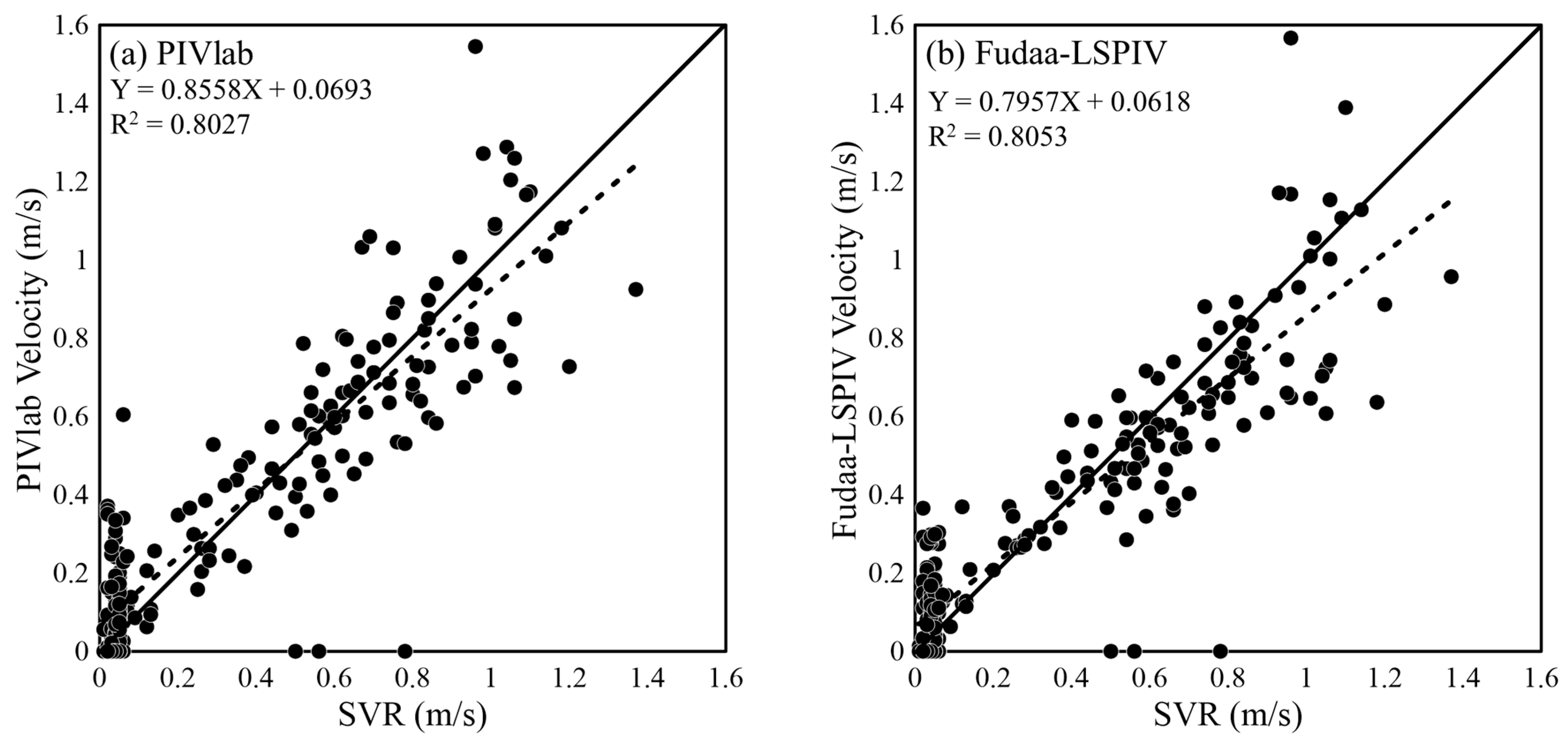
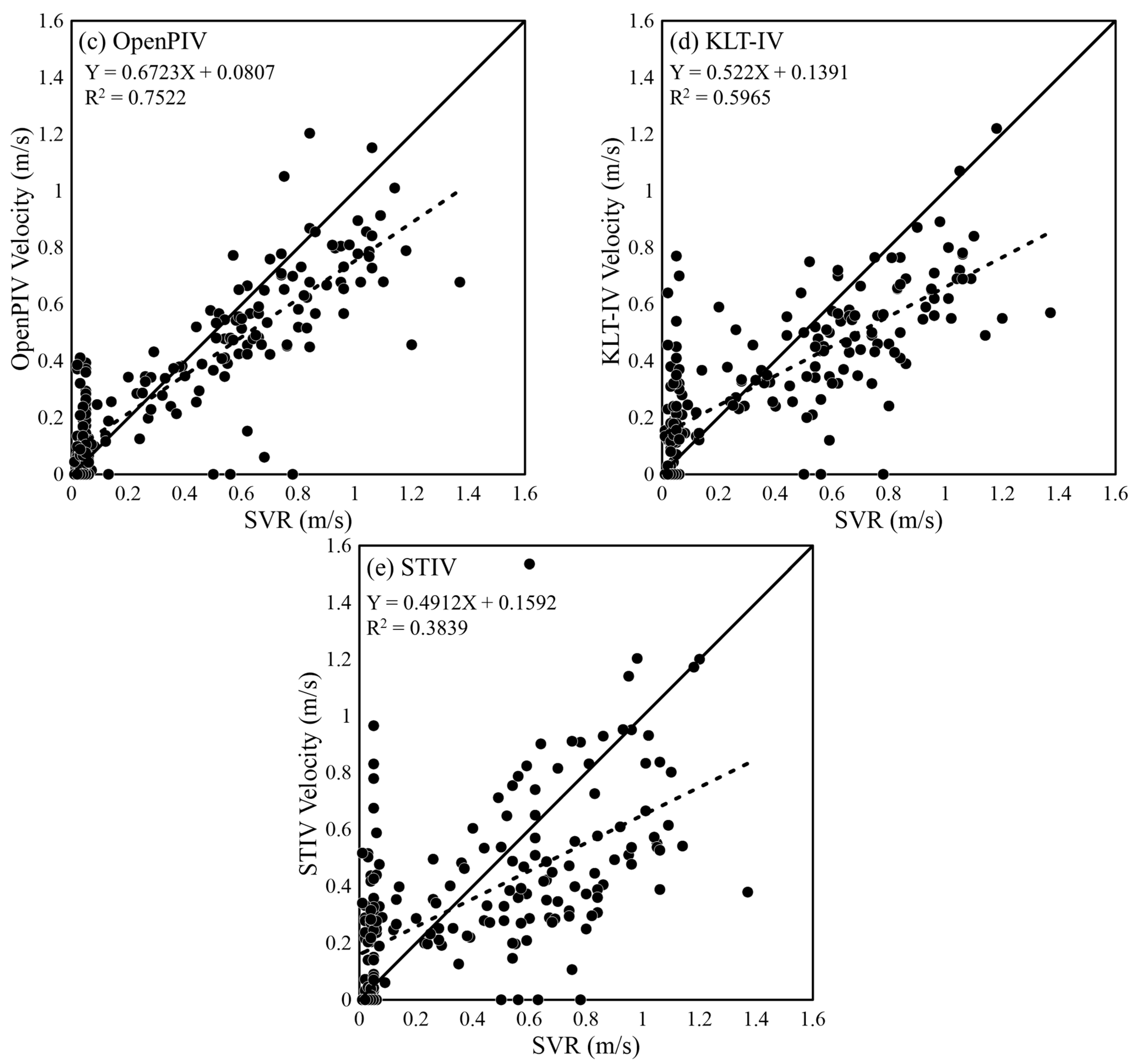
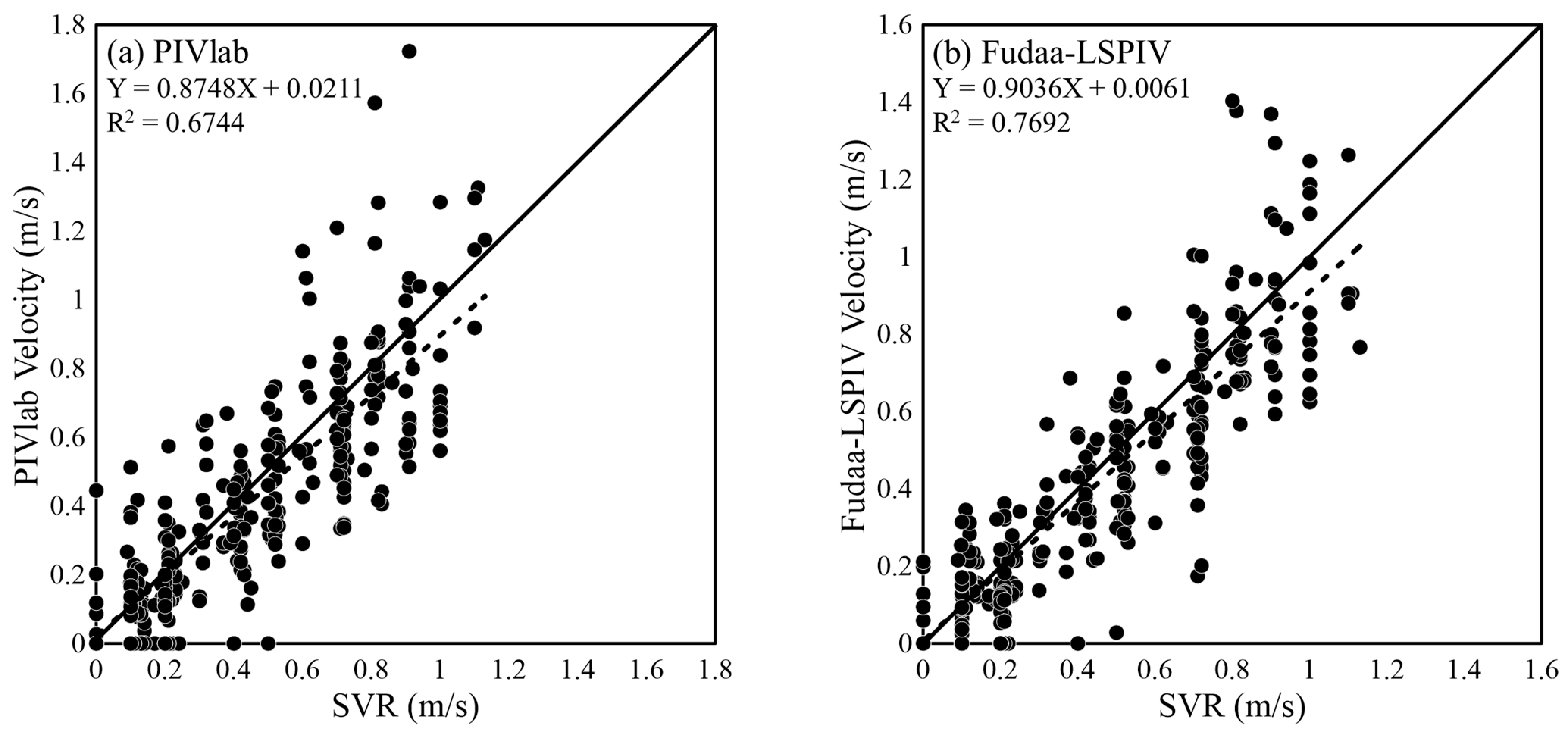
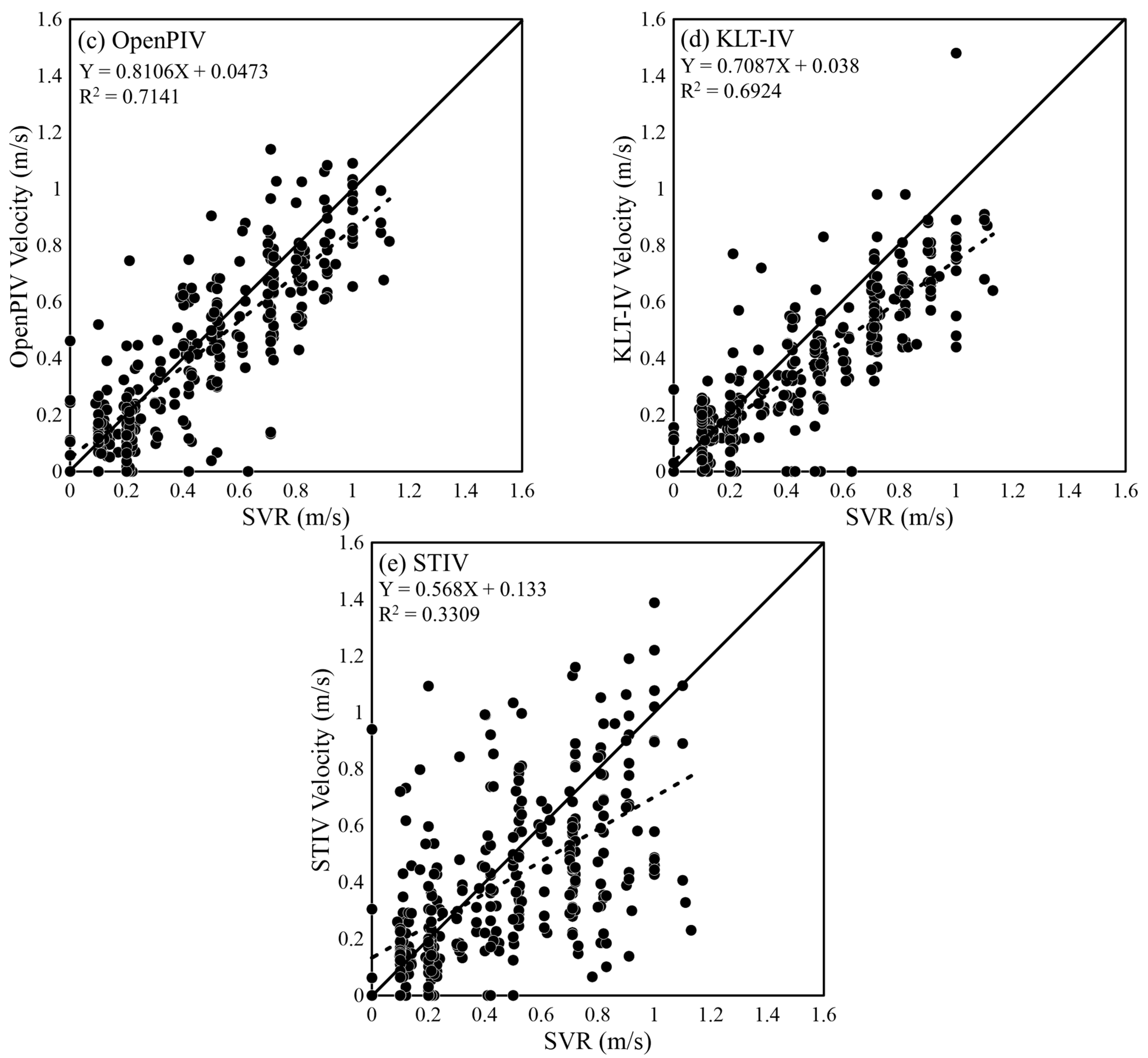
To further analyze the data distribution within each software, Figure 7 depicts a scatter plot comparing SVR and each software. There are 42 points measured each time, and a total of five measurements were taken on that day, resulting in a total of 210 data points. The x = y line indicates a variable tendency of each software to overestimate/underestimate the SVR. Figure 7 shows that Fudaa-LSPIV presents the tendency of least dispersion compared to the other software. The results reveal that Fudaa-LSPIV has the most consistent data distribution, characterized by an R2 value of 0.8053, while STIV shows the highest variability, with an R2 value of 0.3839. Here, R2 represents the coefficient of determination.
3.2. Measurement Results on 11 July 2022
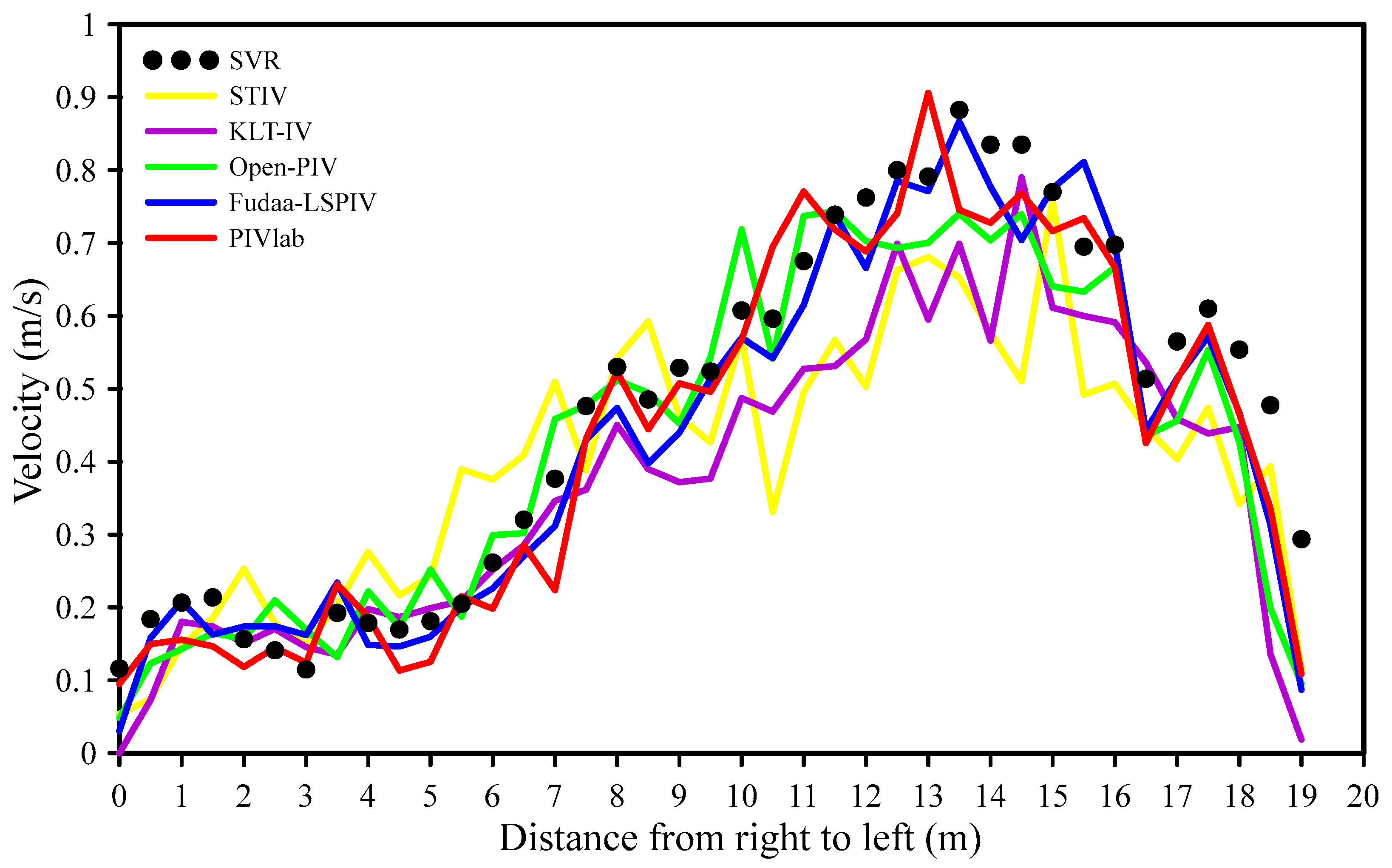
The experiment conducted on 11 July 2022 to collect data occurred from 10 a.m. to 5 p.m., with each video lasting 24 s. The river spanned a length of 19 m, and data points were recorded at 0.5 m intervals, yielding a total of 39 data points. Figure 8 depicts the captured video footage that underwent analysis, resulting in the generation of a flow field for each software. In the overall velocity field analysis results, the average surface velocities for PIVlab, Fudaa-LSPIV, OpenPIV, KLT-IV, and STIV were 0.69 m/s, 0.72 m/s, 0.65 m/s, 0.61 m/s, and 0.62 m/s, respectively. Among all the software types, the maximum difference in the average surface velocity was 0.11 m/s.
An overview of the analysis results obtained from the image velocimetry software is displayed in Figure 9. In general, the velocities obtained across all types of the software remained consistent with those observed in the July 5th experiment, remaining within reasonable limits. Both manual measurements and image velocimetry from this second experiment indicated reasonable results, with water velocity increasing from the riverbank towards the middle of the river. Notably, Fudaa-LSPIV demonstrated the lowest error, with an RMSE of 0.069 m/s and ME of 0.038 m/s.
Figure 10 illustrates a box plot depicting the velocity differences between the image velocimetry software and SVR. The results indicate that the variability between PIVlab, Fudaa-LSPIV, and OpenPIV is not significantly different. However, the box plot reveals that OpenPIV’s maximum and minimum velocity values closely align with SVR’s, resulting in OpenPIV having the shortest whisker. For a more detailed data distribution analysis, see the plots presented in Figure 11, which provide a comparison between the SVR and each software type. It should be noted that each measurement consisted of 39 points, and over the course of the day, a total of eight measurements were conducted, yielding a cumulative dataset of 312 data points. These results suggest that Fudaa-LSPIV exhibited the most consistent data distribution, with an R2 value of 0.7692, while STIV displayed the highest variability, with an R2 value of 0.3309.
Numerous factors exert influences on the outcomes generated by each software package. Both PIVlab and Fudaa-LSPIV conduct orthorectification and enhance the image quality before analysis, resulting in lower errors when compared to the other software options. OpenPIV also employs pre-processing to enhance the image contrast before utilizing a cross-correlation algorithm for analysis. In contrast, STIV is notably affected by variations in light contrast, particularly during the bright conditions observed during the experiments on July 5th and July 11th. These lighting conditions posed challenges for STIV in accurately tracking the movement of the river’s water surface. On the other hand, KLT-IV demands a stable video feed for analysis, as the influence of wind conditions during data collection can cause UAV movement and alter the positions of ground control points, disrupting orthorectification and subsequently impacting the results.
3.3. Influence of the Interrogation Area (IA) on Surface Flow Measurement
After comparing five different software options, it is evident that Fudaa-LSPIV is the most appropriate choice. Consequently, the following subsections exclusively employ Fudaa-LSPIV for water surface velocity analysis. The dataset utilized comprises observations from 16 April, 23 August, and 18 September 2022, acquired through SVR and UAV methods, followed by a comparative analysis. These following subsections aim to ascertain optimal parameters for water surface velocity analysis and assess the impact of artificial particles on the software.
The interrogation area stands as a critical parameter for configuring any image velocimetry software. Understanding the influence of the IA on image velocimetry software and identifying the ideal settings is imperative. The IA’s impact on analysis precision is profound due to its dependence on particle size, with no mathematical formula to universally determine the correct IA for every scenario [34]. Consequently, comparative testing was conducted, involving various IA dimensions—specifically, 64 pixels × 64 pixels, 48 pixels × 48 pixels, 32 pixels × 32 pixels, 16 pixels × 16 pixels, and 8 pixels × 8 pixels—within the context of image velocimetry analysis. All other parameters remained constant, including an image frequency of 12 frames per second and a pixel size of 20.5 mm/pixel; thus, the sole variable under scrutiny was the IA. The dataset used for analysis was obtained on 16 April 2022, between 10 a.m. and 5 p.m. Subsequently, each IA variant was compared to the SVR results.
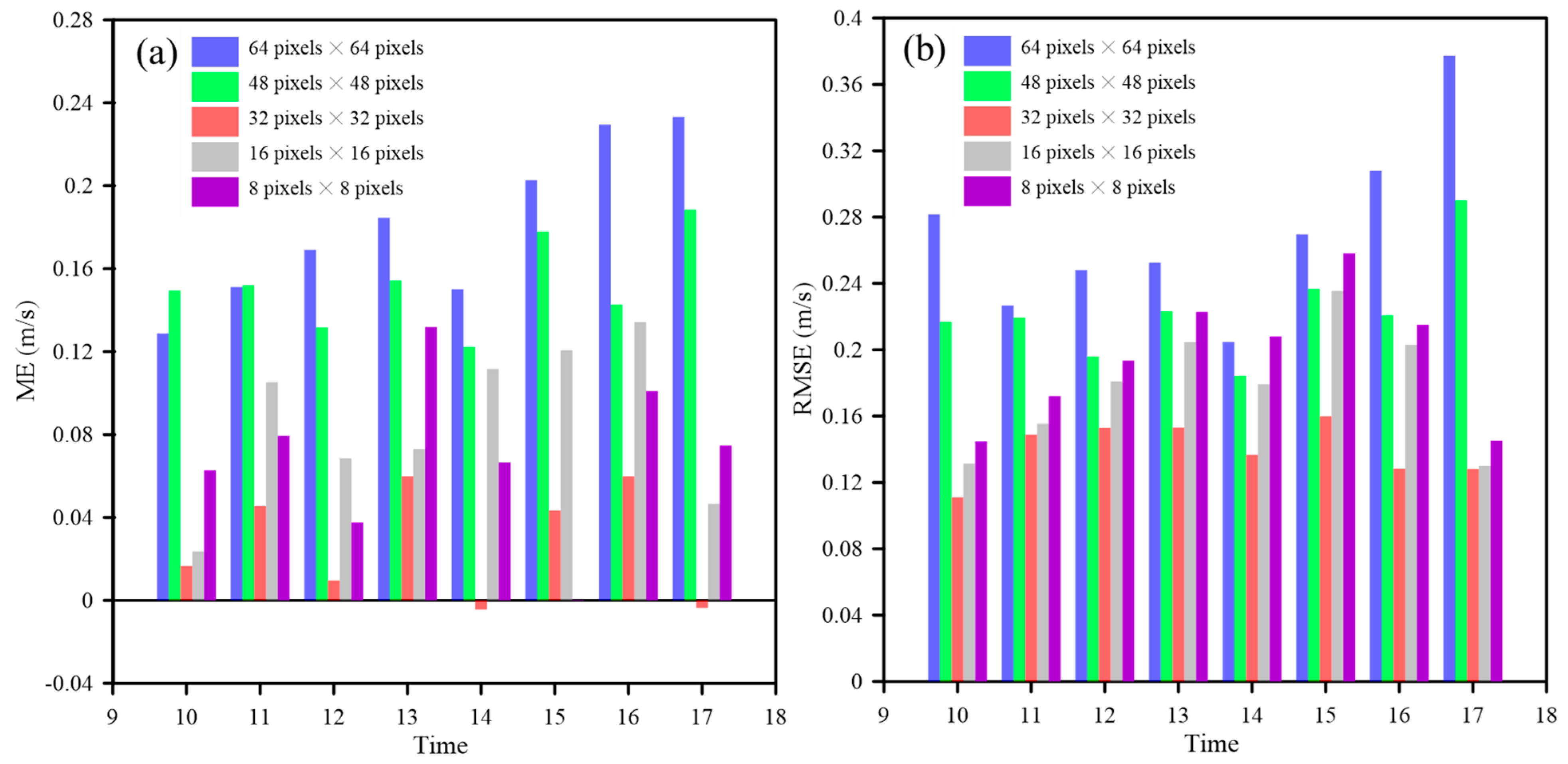
Figure 12 illustrates the statistical error outcomes of the Fudaa-LSPIV analysis for varying IAs. Notably, an IA size of 32 pixels × 32 pixels emerges as the most suitable choice for image velocimetry analysis using Fudaa-LSPIV, as it exhibits the lowest RMSE and ME values over time (Figure 12). Specifically, the average ME and RMSE values for the 32 pixels × 32 pixels IA are 0.03 m/s and 0.14 m/s, respectively. In comparison to IA sizes exceeding 32 pixels × 32 pixels, namely 16 pixels × 16 pixels and 8 pixels × 8 pixels, the latter two dimensions yield better results. This highlights that a larger IA size does not necessarily equate to improved analysis, aligning with the findings of researchers [34], who observed that an oversized IA can compromise velocity vector detection, thus diminishing accuracy. Additionally, these results align with the assertion made by Liu and Huang [2] that a smaller IA does not necessarily enhance measurement precision, as it restricts the search range, leading to successive mismatched images and a subsequent decrease in accuracy or particles escaping from the IA if it is too small. Consequently, it is essential to tailor the IA size to the particle size in order to optimize the output results.
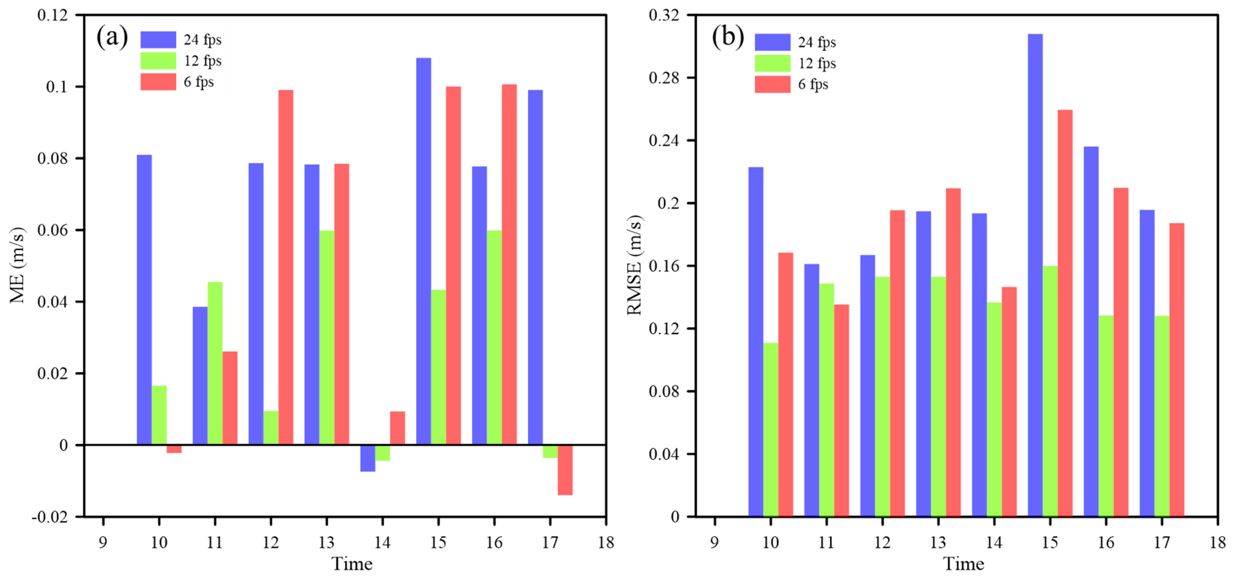
3.4. Influence of Image Frequency on Surface Flow Measurement
The input videos utilized for analysis exhibit varying frame rates or image frequencies. The movement of particles within the physical space, as captured in the image frames, is notably influenced by the acquisition frame rate. Subsequently, these particles motions undergo analysis through image velocimetry, as highlighted in the study by Caridi et al. [35]. Consequently, a comparative examination was conducted using distinct image frequencies—specifically, 24 fps, 12 fps, and 6 fps—aimed at determining the image frequencies that yield the most suitable results. If the image frequency is excessively fast or slow, the inter-frame particles displacement becomes imperceptible, as noted by Pearce et al. [4]. Other parameters remained constant, encompassing an IA of 32 pixels × 32 pixels and a pixel size of 20.5 mm/pixel. The temporal data chosen for analysis spanned from 10 a.m. to 5 p.m. on 16 April 2022. Each instance with a distinct image frequency was juxtaposed with the SVR outcomes.
The findings of this analysis are graphically presented in Figure 13, illustrating the statistical error outcomes of the Fudaa-LSPIV analysis across different image frequencies. This graph discerns that videos with either higher or lower frame rates yield more precise results. Notably, videos or images captured at 12 fps exhibited the most favorable outcomes during the 10 a.m. to 5 p.m. timeframe compared to their counterparts. Figure 13 explicitly showcases that the average ME and RMSE values with a 12 fps video are 0.03 m/s and 0.14 m/s, respectively. This substantiates the assertion that the frame rate of the video or image significantly influences the outcomes of image velocimetry analysis.
3.5. Influence of Pixel Size on Surface Flow Measurement
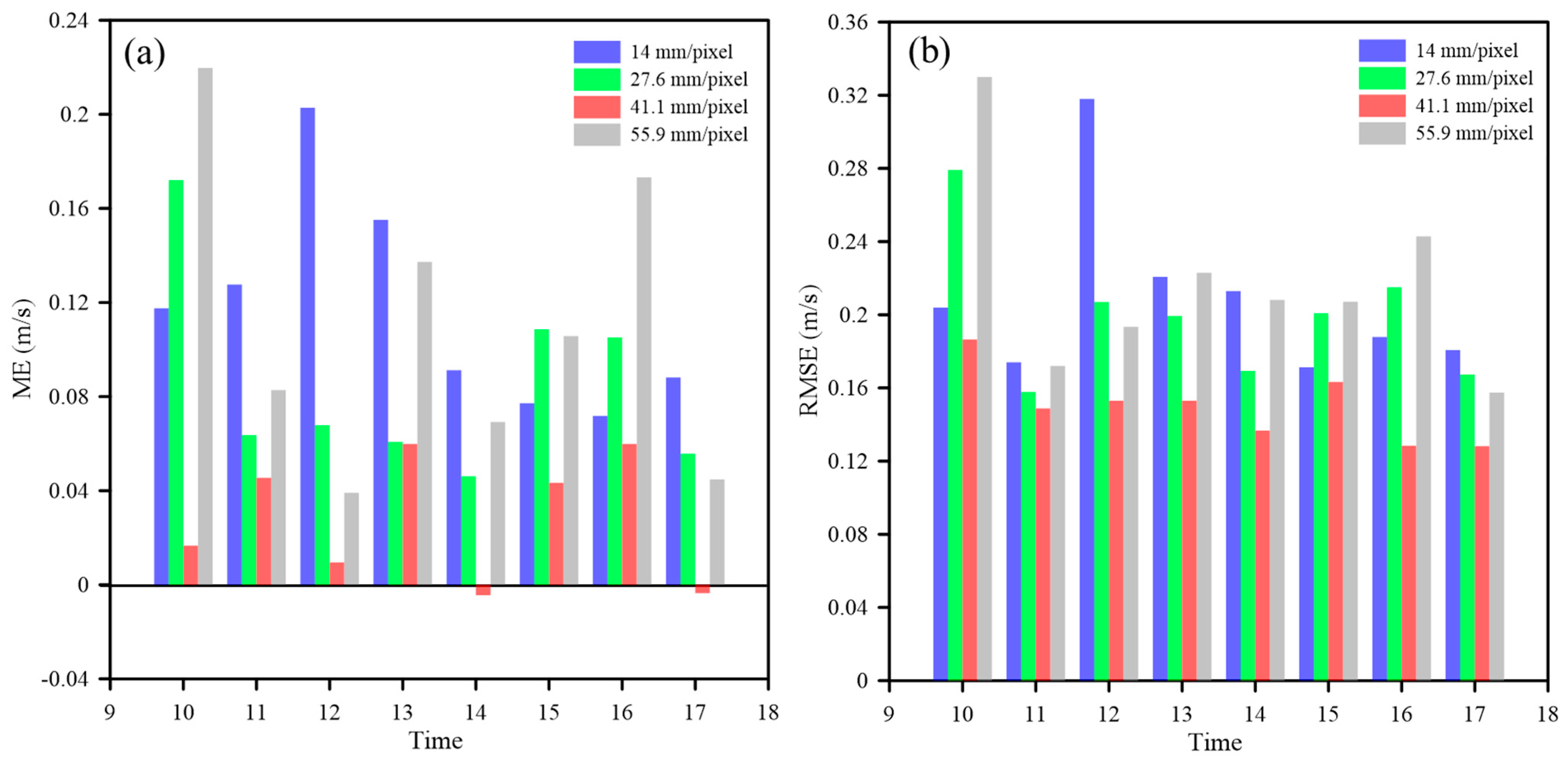
The video used for analysis was captured using an unmanned aerial vehicle (UAV), and as a result, the UAV’s altitude has a significant impact on the analysis outcomes. Variations in the UAV’s altitude influence the clarity of the particles observed on the water’s surface in the video. Liu and Huang [2] pointed out that higher UAV altitudes can adversely affect image resolution. They also demonstrated that the mean absolute error (MAE) value was lowest for the UAV at an altitude of 62 m, compared to those at altitudes of 32 m and 112 m. These findings suggest that a lower UAV flying altitude does not necessarily yield superior results.
To investigate the optimal UAV altitude for image velocimetry analysis, an experiment was conducted with different UAV heights: specifically, 15 m, 35 m, 55 m, and 75 m. The pixel sizes at flying heights of 15 m, 35 m, 55 m, and 75 m are 7 mm/pixel, 13.8 mm/pixel, 20.5 mm/pixel, and 27.4 mm/pixel, respectively. At a flying height of 15 m, the captured image range can cover the entire width of the river. Other parameters remained constant, including an IA of 32 pixels × 32 pixels and an image capture rate of 12 fps. The dataset utilized for analysis comprised data from 16 April 2022, spanning from 10 a.m. to 5 p.m. Each pixel size was compared with SVR results.
Figure 14 illustrates the statistical error results of the Fudaa-LSPIV analysis for various pixel sizes. Notably, a pixel size of 20.5 mm/pixel produced the most favorable outcomes between 10 a.m. and 5 p.m. The average ME and RMSE values at a pixel size of 20.5 mm/pixel were 0.03 m/s and 0.140 m/s, respectively. These results indicate that the altitude at which the UAV operates significantly influences the accuracy of image velocimetry analysis.
3.6. Influence of Artificial Particles on Surface Flow Measurement
We conducted parameter adjustments involving an internal LSPIV parameter (IA) and video data parameters (pixel size and image frequency) by varying these parameters and comparing the analysis results to determine the most suitable values for the Xihu River scenario. Our analysis employed an IA setting of 32 pixels × 32 pixels, a pixel size of 20.5 mm/pixel, and an image frequency of 12 fps. The data used in these experiments were collected on August 23 and 18 September 2022. The analysis was performed using the Fudaa-LSPIV software. In these experiments, we conducted analyses both with and without artificial particles, specifically wood shavings, for water surface velocity analysis, and we compared the results with those obtained using SVR. Some of the characteristics of wood shavings are its light weight, small volume, easy visibility (i.e., large surface area and unique color), biodegradability, environmental neutrality, and low cost, making them suitable for use as tracers [36].
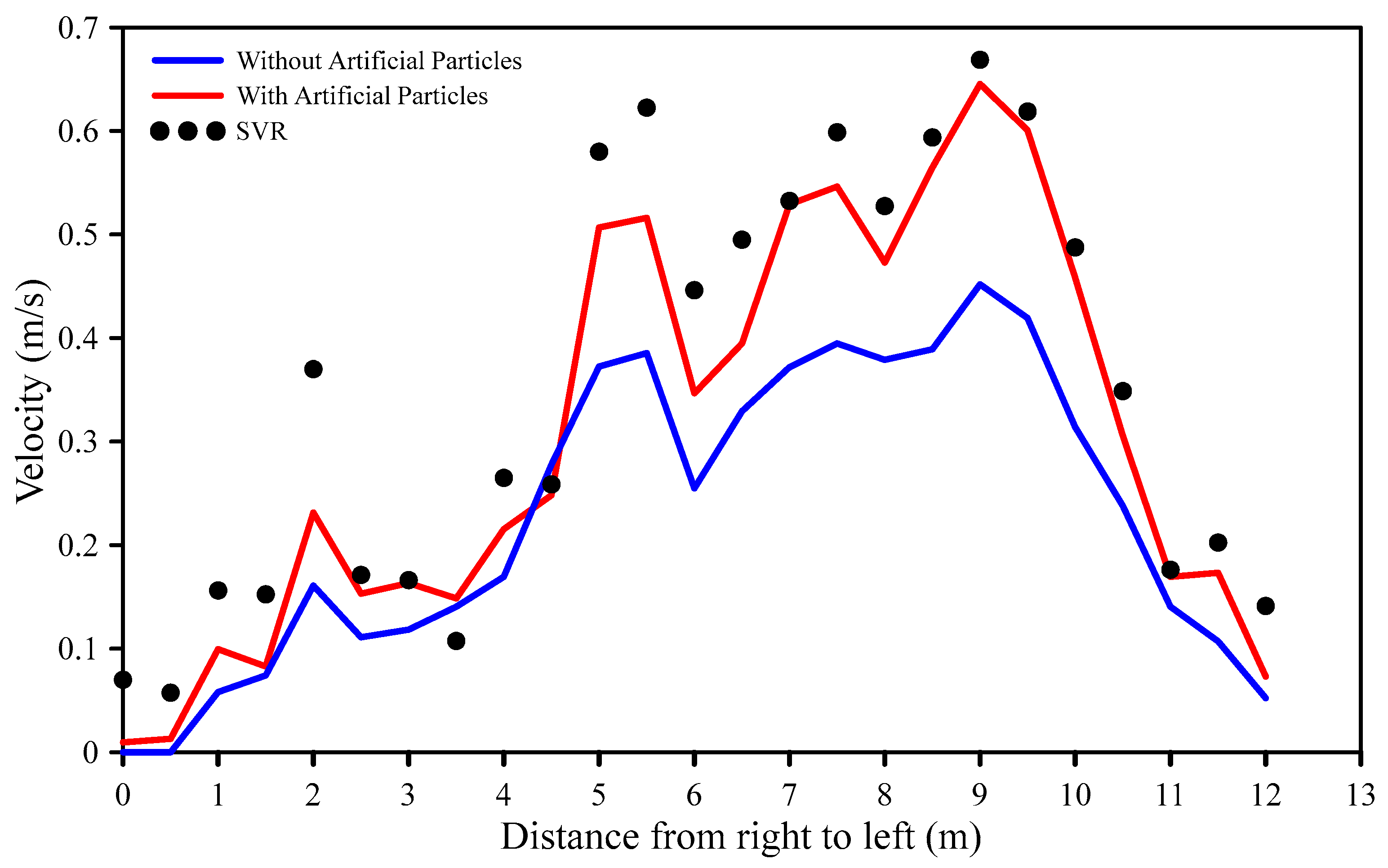
On 23 August 2022, field trials were conducted under conditions deemed safe for manual measurements in the river. Data collection took place from 9 a.m. to 4 p.m., with video recordings lasting for 40 s each. The river’s shallowness limited its length to approximately 12 m, with data measurements taken at 0.5 m intervals using SVR. Data were initially collected using SVR and subsequently subjected to analysis using Fudaa-LSPIV. Figure 15 provides measurements taken along cross-sectional lines. In the seeding section (ranging from a distance of 5 m to 10 m), the water’s surface velocity without artificial particles was observed to be lower than that with artificial particles. This observation indicates that artificial particles enhance Fudaa-LSPIV’s ability to detect the movement of surface water particles. The differences in the ME and RMSE values between the analyses with artificial particles and those without were approximately 0.099 m/s and 0.092 m/s, respectively.
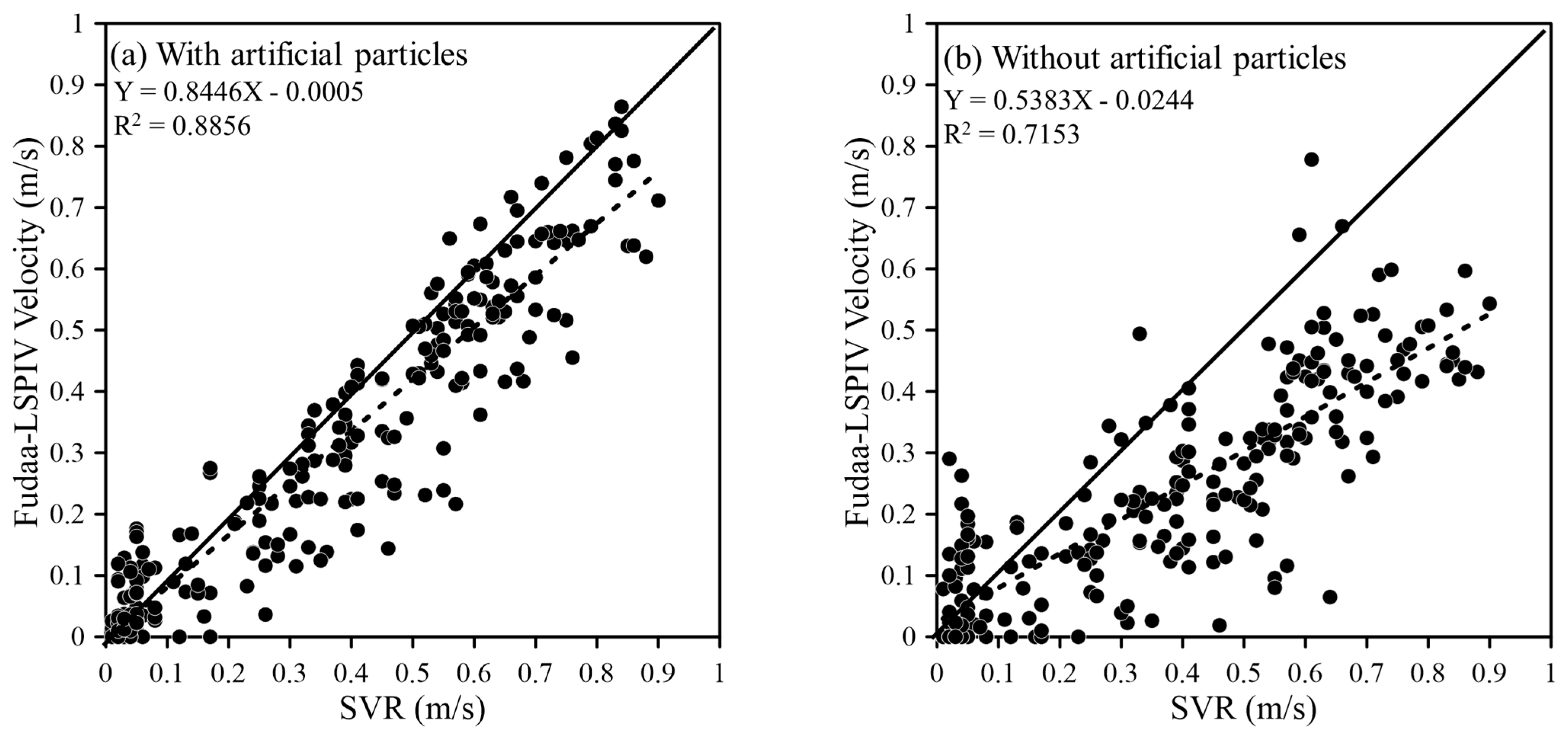
For a more comprehensive examination of the data distribution, Figure 16 presents a comparison of the SVR and Fudaa-LSPIV analyses, both with and without artificial particles. The data reveal that the deviations in the analysis with artificial particles are smaller than those without. In terms of regression analysis values, the presence of artificial particles yielded a value of 0.8856, while the absence of artificial particles resulted in a value of 0.7153.
On 18 September 2022, field trials were conducted under conditions deemed safe for manual measurements in the river. Data collection occurred from 9 a.m. to 4 p.m., with each video recording lasting for 40 s. The river’s relatively shallow depth allowed for a longer river length compared to August 18, spanning approximately 14 m, with data measurements taken at 0.5 m intervals using SVR.
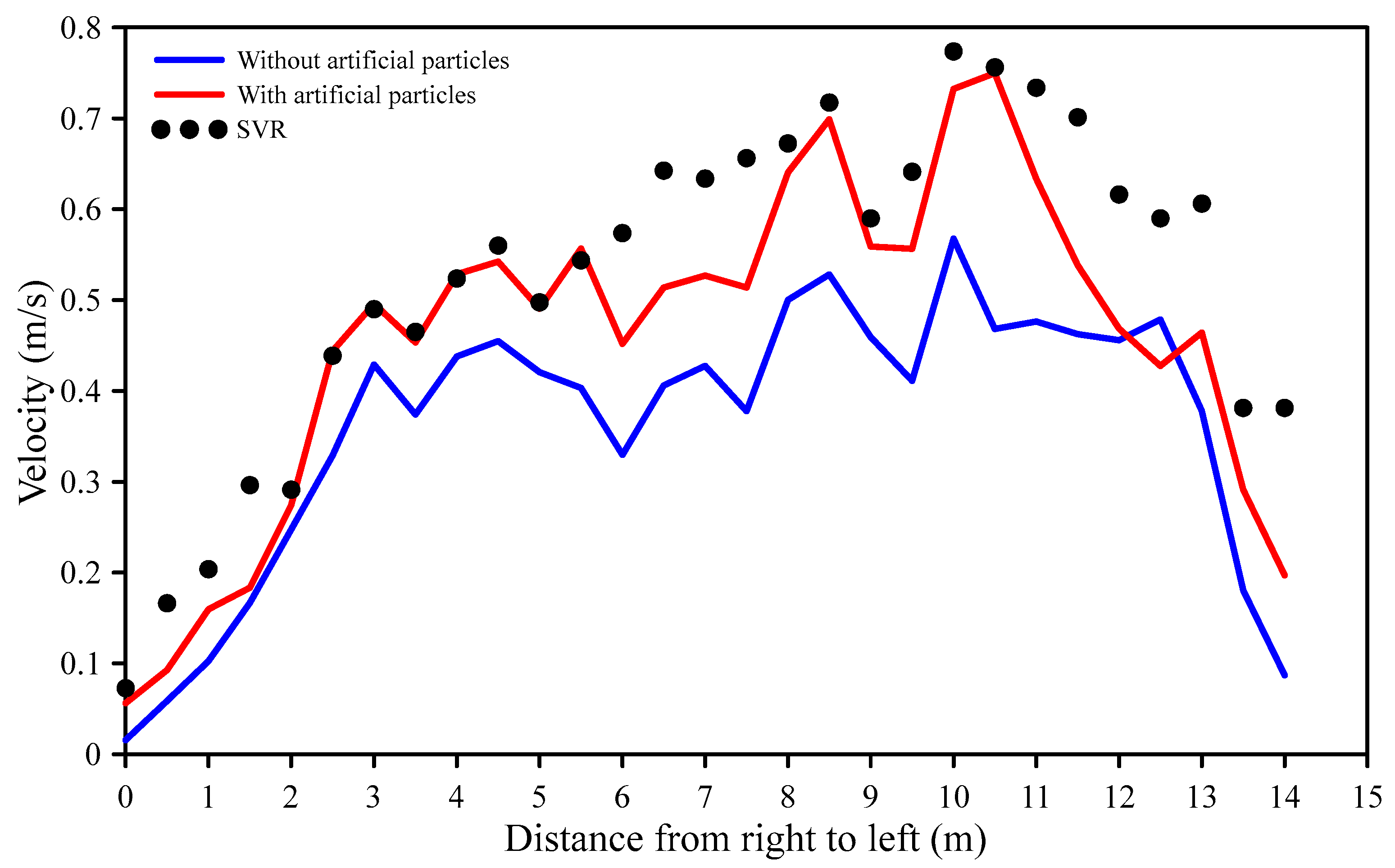
Figure 17 portrays the measurement results along cross-sectional lines. In the seeding portion, specifically the left side of the river (ranging from 5 m to 10 m), the water’s surface velocity without artificial particles was observed to be lower than that with artificial particles. Further downstream (between 10 m and 13 m), an area where artificial particles were introduced, the water surface velocity was slightly lower than the SVR measurements. This suggests that artificial particles enhance Fudaa-LSPIV’s capacity to detect the motion of surface water particles. The differences in the ME and RMSE values between the analyses with artificial particles and those without were approximately 0.087 m/s and 0.086 m/s, respectively.
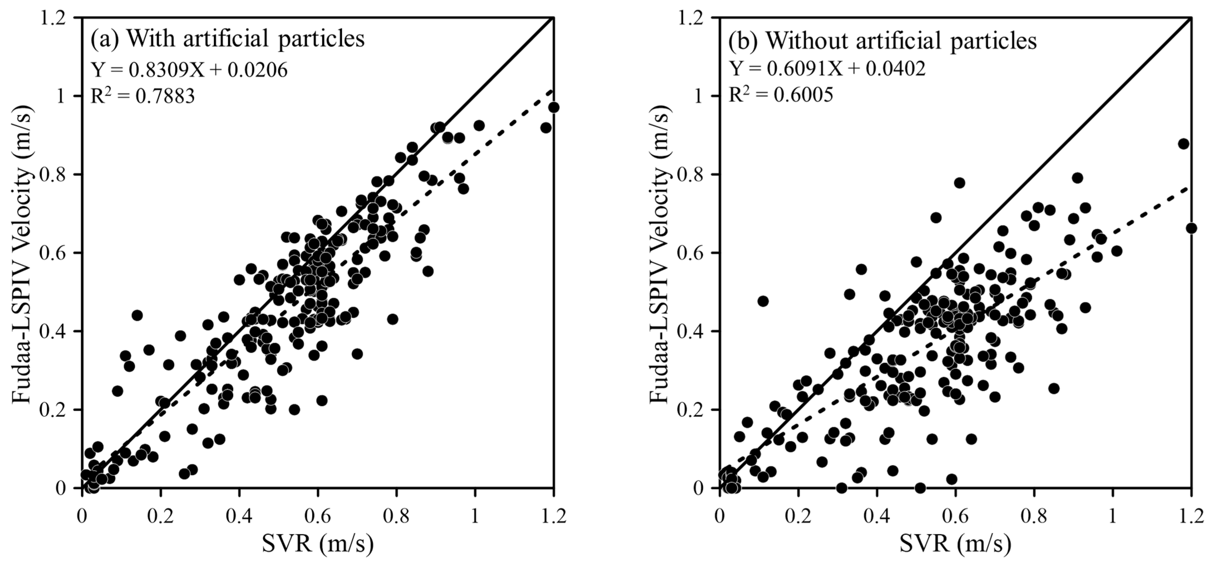
For a more in-depth examination of the data distribution, Figure 18 presents a comparison between SVR and Fudaa-LSPIV analyses, both with and without artificial particles. It suggests that deviations in the analysis with artificial particles are smaller than those in the analysis without. In terms of regression analysis values, the presence of artificial particles yielded a value of 0.788, while the absence of artificial particles resulted in a value of 0.601.
Both the experiments conducted on August 23 and September 18 in 2022 consistently demonstrated that the Fudaa-LSPIV analysis results with artificial particles outperformed those without, showcasing lower ME and RMSE values. This substantiates the assertion made by Dal Sasso et al. [30,37] that the inclusion of artificial particles enhances the accuracy of detecting water surface particles movements. Furthermore, the research conducted on these two dates revealed that the surface velocity results obtained from Fudaa-LSPIV analysis remained below the SVR measurements, especially in areas not traversed by artificial particles. The observed lower ME and RMSE values on August 23 compared to September 18 can be attributed to differences in the dispersion of artificial particles within the river and higher river flow rates on September 18 in contrast to August 23. Elevated river flow rates cause artificial particles to move more swiftly, and since the video’s duration was only 30−40 s, it may capture areas devoid of artificial particles. Reducing the video duration would result in a reduction in frames available for analysis, potentially impacting the overall accuracy of the results.
4. Discussion
4.1. Specific Measurement on 11 July 2022
The software employing the PIV algorithm consistently exhibits lower errors than their counterparts. While all three utilize the same algorithm, the techniques employed during the analysis stage by these software options yield variations in the resulting water surface velocity. Consequently, it becomes imperative to conduct comparisons that extend beyond solely relying on the ME and RMSE values.
Drawing insights from Figure 4 and Figure 8, it becomes evident that KLT-IV’s flow field exhibits the greatest irregularities compared to the other software, a phenomenon influenced by factors such as ground control points and camera positioning. Because KLT-IV image alignment takes into account both the GCPs and camera position, unlike other software that only considers GCPs. Therefore, the movement of the UAV has a direct impact on both the camera and ground control point locations, resulting in the formation of larger vectors that do not align in a uniform direction. This issue can be mitigated by exercising control over the ground control point placement during the analysis and adjusting the extraction rate, which, in turn, affects the number of generated trajectories. It should be noted that the analysis results of PIVlab, STIV, and OpenPIV have all been corrected using the RIVeR software to eliminate the effects of instability in aerial UAV video recording. In contrast, Fudaa-LSPIV and KLT-IV have built-in correction procedures.
Despite these variations, all software packages produce results with consistent flow directions, rendering them acceptable for analysis purposes. Among all software packages, the flow direction of STIV is more consistent than other software, because STIV is a one-dimensional water velocity calculation method that uses the image surface in a search line as an object of analysis in a space-time image [38]. Therefore, while STIV can be used to measure the surface flow velocity of rivers, it is not suitable for studying changes in river surface flow patterns. Notably, STIV stands out as particularly challenging due to its sensitivity to changes in image brightness, leading to hourly adjustments in applied filters based on the field conditions. Furthermore, the size of the search line influences the light captured for analysis; if it primarily captures darker areas, the image analysis window becomes dominated by these dark regions.
Fudaa-LSPIV emerges as the most suitable software for analysis, boasting the lowest ME and RMSE values compared to the other software in the experiments conducted on 5 and 11 July 2022. Delving into the vector fields, it becomes apparent that the vectors in STIV exhibit greater stability when contrasted with those in Fudaa-LSPIV. This is mainly because the analysis results of STIV represent a one-dimensional flow field, so all velocity vectors point in the same direction. In contrast, Fudaa-LSPIV, OpenPIV, PIVlab, and KLT-IV generate vector fields across all analyzed river areas. Consequently, vectors in these areas become more concentrated along the red line, facilitating comparisons with SVR values. In this regard, Fudaa-LSPIV demonstrates a balanced vector distribution, predominantly in an upward direction, with a more consistent orientation when contrasted with PIVlab, which primarily exhibits a single direction (as depicted in Figure 8). When looking at the box plots in Figure 6, it is evident that PIVlab produces the most compact data distribution, while OpenPIV achieves the same in Figure 10. Moving on to the scatter plots, Fudaa-LSPIV presents the most regular data distribution with the least dispersion when compared to the other software (as illustrated in Figure 7 and Figure 10). This is further corroborated by the highest R2 values observed in Figure 7 and Figure 11. All of these factors collectively affirm that Fudaa-LSPIV is the most appropriate software for conducting the analysis in this study.
4.2. Advantages, Limitations, and Future Work
Our comparison of five different software packages reveals variations in their usage, leading to distinct strengths and weaknesses. The accuracy of the KLT-IV trajectory results is significantly impacted by factors such as camera positioning and UAV shake, whereas STIV is influenced by the brightness levels. PIVlab, Fudaa-LSPIV, and OpenPIV all employ the same PIV algorithm, utilizing cross-correlation, resulting in fairly consistent ME and RMSE values. The PIV algorithm assesses particles motion through a sequence of images, employing multiple passes and pre-processing/post-processing to enhance particles tracking precision. A detailed breakdown of the pros and cons of each software can be found in Table 3.
While using a UAV can provide more accurate and straightforward results, it does have limitations, particularly in terms of video duration. Expanding from simple measurements to real-time velocity monitoring necessitates a stable and durable camera system. The images captured with the camera are directly transmitted to and processed with a computer for calculating the water surface velocity. Additionally, adverse weather conditions, such as rain, can pose challenges when recording data with a UAV. There is also potential for the development of other image velocimetry techniques, including the application of deep learning for water surface velocity detection.
Deep learning techniques, such as convolutional neural networks (CNNs), can be employed to extract spatial features from images, although their effectiveness may vary depending on the complexity of the problem. Deep learning models utilize images as their input data and produce velocity fields as their output data. The implementation of deep learning can be achieved on a small scale, such as in a laboratory setting, with conditions tailored to field-specific requirements [39,40].
5. Conclusions
A comprehensive assessment was conducted of the Xihu River to measure its water surface velocity using UAV technology, focusing on five distinct software programs: PIVlab, Fudaa-LSPIV, OpenPIV, KLT-IV, and STIV. The primary objective was to evaluate the performance of these software programs. This evaluation took place during two trials, held on 5 July and 11 July 2022, with SVR serving as the benchmark. Throughout both trials, consistent parameters were maintained for all software programs, including an IA size of 32 pixels × 32 pixels, a pixel size of 20.5 mm/pixel, and an image frequency of 12 fps. The analysis results revealed that all software programs produced acceptable results. However, the software employing the PIV algorithm demonstrated a lower statistical error value. Among the five software programs, Fudaa-LSPIV consistently exhibited the lowest ME and RMSE values in both trials. It also displayed superior scatter plot and box plot results, characterized by low regression and scatter values.
To explore the influence of the IA, image frequency, and pixel size parameters on water surface velocity analysis, the Fudaa-LSPIV software was specifically utilized. This trial was conducted using data gathered on 16 April 2022. The comparison revealed that the combination of an IA size of 32 pixels × 32 pixels, an image frequency of 12 fps, and a pixel size of 20.5 mm/pixel yielded the most favorable results.
In a separate investigation employing Fudaa-LSPIV, the study delved into the impact of introducing artificial particles on the precision of water surface velocity measurements. The parameters selected for this analysis were derived from previous trials, incorporating an IA of 32 pixels × 32 pixels, an image frequency of 12 fps, and a pixel size of 20.5 mm/pixel. This experimental research was carried out over two days, specifically on August 23 and 18 September 2022. The results demonstrated that the incorporation of artificial particles significantly enhanced the detection of the water’s surface movements. In these scenarios, the inclusion of artificial particles proved to be a valuable asset, enabling Fudaa-LSPIV to effectively identify patterns on the water surface.
Author Contributions
Conceptualization, W.-C.L. and W.-C.H.; methodology, W.-C.H. and F.W.; software, F.W.; validation, W.-C.L., S. and W.-C.H.; formal analysis, F.W.; investigation, W.-C.L. and S.; resources, W.-C.L.; data curation, F.W. and W.-C.H.; writing—W.-C.L. and F.W.; original draft preparation, F.W.; writing—review and editing, W.-C.L. and S.; visualization, F.W.; supervision, W.-C.L. and S.; project administration, W.-C.L. and W.-C.H.; funding acquisition, W.-C.L. All authors have read and agreed to the published version of the manuscript.
Funding
This present study was partially funded by the National Science and Technology Council, Taiwan (MOST 111-2625-M-239-001).
Data Availability Statement
Data are contained within the article.
Acknowledgments
This investigation received partial financial backing from the National Science and Technology Council, Taiwan. The authors extend their sincerest appreciation for this support.
Conflicts of Interest
The authors declare no conflict of interest.
References
- Yu, K.; Lee, J. Method for measuring the surface velocity field of a river using images acquired by a moving drone. Water 2023, 15, 53. [Google Scholar] [CrossRef]
- Liu, W.C.; Huang, W.C. Development of a three-axis accelerometer and large-scale particle image velocimetry (LSPIV) to enhance surface velocity measurements in rivers. Comput. Geosci. 2021, 155, 104866. [Google Scholar] [CrossRef]
- Eltner, A.; Sardemann, H.; Grundmann, J. Technical note: Flow velocity and discharge measurement in rivers using terrestrial and unmanned-aerial-vehicle imagery. Hydrol. Earth Syst. Sci. 2020, 24, 1429–1445. [Google Scholar] [CrossRef]
- Pearce, S.; Ljubicic, R.; Peña-Haro, S.; Perks, M.; Tauro, F.; Pizarro, A.; Dal Sasso, S.F.; Strelnikova, D.; Grimaldi, S.; Maddock, I.; et al. An evaluation of image velocimetry techniques under low flow conditions and high seeding densities using unmanned aerial systems. Remote Sens. 2020, 12, 232. [Google Scholar] [CrossRef]
- Jolley, M.J.; Russell, A.J.; Quinn, P.F.; Perks, M.T. Considerations when applying Large-Scale PIV and PTV for determining river flow velocity. Front. Water 2021, 3, 709269. [Google Scholar] [CrossRef]
- Bandini, F.; Frías, M.C.; Liu, J.; Simkus, K.; Karagkiolidou, S.; Bauer-Gottwein, P. Challenges with regard to Unmanned Aerial Systems (UASs) measurement of river surface velocity using Doppler radar. Remote Sens. 2022, 14, 1277. [Google Scholar] [CrossRef]
- Hou, J.; Yang, L.; Wang, X.; Chai, J.; Zhang, Z.; Li, X.; Shao, J.; Du, Y.; Bai, G. Adaptive large-scale particle image velocimetry method for physical model experiments of flood propagation with complex flow patterns. Measurement 2022, 198, 111309. [Google Scholar] [CrossRef]
- Rozos, E.; Mazi, K.; Koussis, A.D. Probabilistic evaluation and filtering of image velocimetry measurements. Water 2021, 13, 2206. [Google Scholar] [CrossRef]
- Masafu, C.; Williams, R.; Shi, X.; Yuan, Q.; Trigg, M. Unpiloted Aerial Vehicle (UAV) image velocimetry for validation of two-dimensional hydraulic model simulations. J. Hydrol. 2022, 612, 128217. [Google Scholar] [CrossRef]
- Ljubičić, R.; Strelnikova, D.; Perks, M.T.; Eltner, A.; Penã-Haro, S.; Pizarro, A.; Dal Sasso, S.F.; Scherling, U.; Vuono, P.; Manfreda, S. A comparison of tools and techniques for stabilising unmanned aerial system (UAS) imagery for surface flow observations. Hydrol. Earth Syst. Sci. 2021, 25, 5105–5132. [Google Scholar] [CrossRef]
- Thielicke, W.; Stamhuis, E.J. PIVlab—Towards user-friendly, affordable and accurate digital particle image velocimetry in MATLAB. J. Open Res. Softw. 2014, 2, 30. [Google Scholar] [CrossRef]
- Ben-Gida, H.; Gurka, R.; Liberzon, A. OpenPIV-MATLAB-An open-source software for particle image velocimetry; test case: Birds’ aerodynamics. SoftwareX 2020, 12, 100585. [Google Scholar] [CrossRef]
- Le Coz, J.; Jodeau, M.; Hauet, A.; Marchand, B.; Boursicaud, R. Image-based velocity and discharge measurements in field and laboratory river engineering studies using the free FUDAA-LSPIV software. Proc. Intern. Conf. Fluv. Hydraul. River Flow 2014, 2014, 1961–1967. [Google Scholar]
- Jodeau, M.; Le Coz, J.; Bercovitz, Y.; Lebert, F. Laboratory and field lspiv measurements of flow velocities using Fudaa-LSPIV a free user-friendly software Fudaa-lspiv: A user friendly software View project Passive Acoustic Monitoring View project. In Proceedings of the HydroSensoft Conference, HydroSenSoft, International Symposium and Exhibition on Hydro-Environment Sensors and Software, Madrid, Spain, 1–3 March 2017. [Google Scholar]
- Perks, M.T. KLT-IV v1.0: Image velocimetry software for use with fixed and mobile platforms. Geosci. Model Dev. 2020, 13, 6111–6130. [Google Scholar] [CrossRef]
- Fujita, I.; Watanabe, H.; Tsubaki, R. Development of a non-intrusive and efficient flow monitoring technique: The space-time image velocimetry (STIV). Int. J. River Basin Manag. 2007, 5, 105–114. [Google Scholar] [CrossRef]
- Patalano, A.; García, C.M.; Rodríguez, A. Rectification of image velocity results (RIVeR): A simple and user-friendly toolbox for large scale water surface particle image velocimetry (PIV) and particle tracking velocimetry (PTV). Comput. Geosci. 2017, 109, 323–330. [Google Scholar] [CrossRef]
- Fujita, I.; Notoya, Y.; Tani, K.; Tateguchi, S. Efficient and accurate estimation of water surface velocity in STIV. Environ. Fluid Mech. 2019, 19, 1363–1378. [Google Scholar] [CrossRef]
- Lu, J.; Yang, X.; Wang, J. Velocity vector estimation of two-dimensional flow field based on STIV. Sensors 2023, 23, 955. [Google Scholar] [CrossRef]
- Hutley, N.R.; Beecroft, R.; Wagenaar, D.; Soutar, J.; Edwards, B.; Deering, N.; Grinham, A.; Albert, S. Adaptively monitoring streamflow using a stereo computer vision system. Hydrol. Earth Syst. Sci. 2023, 27, 2051–2073. [Google Scholar] [CrossRef]
- Tauro, F.; Petroselli, A.; Arcangeletti, E. Assessment of drone-based surface flow observations. Hydrol. Proc. 2016, 30, 1114–1130. [Google Scholar] [CrossRef]
- Huang, W.C.; Young, C.C.; Liu, W.C. Application of an automated discharge imaging system and LSPIV during typhoon events in Taiwan. Water 2018, 10, 280. [Google Scholar] [CrossRef]
- Liu, W.C.; Lu, C.H.; Huang, W.C. Large-scale particle velocimetry to measure streamflow from videos from unmanned aerial vehicle and fixed imaging system. Remote Sens. 2021, 13, 2661. [Google Scholar] [CrossRef]
- Pena-Haro, S.; Carrel, M.; Luthi, B.; Hansen, I.; Lukes, R. Robust image-based streamflow measurements for real-time continuous monitoring. Front. Water 2021, 3, 766918. [Google Scholar] [CrossRef]
- Lewis, Q.W.; Rhoads, B.L. LSPIV measurements of two-dimensional flow structure in stream using small unmanned aerial systems: 2. Hydrodynamic mapping at river confluences. Water Resour. Res. 2018, 54, 7891–7999. [Google Scholar] [CrossRef]
- Acharya, B.S.; Bhandari, M.; Bandini, F.; Pizarro, A.; Perks, M.; Joshi, D.R.; Wang, S.; Dogwiler, T.; Ray, R.L.; Kharel, G.; et al. Unmanned aerial vehicles in hydrology and water management: Applications, challenges, and perspectives. Water Resour. Res. 2021, 57, e2021WR029925. [Google Scholar] [CrossRef]
- Eskandari, R.; Mahdianpari, M.; Mohammadimanesh, F.; Salehi, B.; Brisco, B.; Homayouni, S. Meta-analysis of unmanned aerial vehicle (UAV) imagery for agro-environmental monitoring using machine learning and statistical models. Remote Sens. 2020, 12, 3511. [Google Scholar] [CrossRef]
- Federman, A.; Shrestha, S.; Quintero, M.S.; Mezzino, D.; Gregg, J.; Kretz, S.; Ouimet, C. Unmanned Aerial Vehicles (UAV) photogrammetry in the conservation of historic places: Carleton Immersive Media Studio case studies. Drones 2018, 2, 18. [Google Scholar] [CrossRef]
- Strelnikova, D.; Paulus, G.; Käfer, S.; Anders, K.H.; Mayr, P.; Mader, H.; Scherling, U.; Schneeberger, R. Drone-based optical measurements of heterogeneous surface velocity fields around fish passages at hydropower dams. Remote Sens. 2020, 12, 384. [Google Scholar] [CrossRef]
- Dal Sasso, S.F.; Pizarro, A.; Manfreda, S. Metrics for the quantification of seeding characteristics to enhance image velocimetry performance in rivers. Remote Sens. 2020, 12, 1789. [Google Scholar] [CrossRef]
- Legleiter, C.; Kinzel, P. Inferring surface flow velocities in sediment-laden Alaskan Rivers from optical image sequences acquired from a helicopter. Remote Sens. 2020, 12, 1282. [Google Scholar] [CrossRef]
- Welber, M.; Le Coz, J.; Jonathan, B.L.; Zolezzi, G.; Zamler, D.; Dramais, G.; Hauet, A.; Salvaro, M. Field assessment of noncontact stream gauging using portable surface velocity radars (SVR). Water Resour. Res. 2016, 52, 1108–1126. [Google Scholar] [CrossRef]
- Son, G.; Kim, D.; Kim, K.; Roh, Y. Performance of a rectangular-shaped surface velocity radar for river velocity measurements. KSCE J. Civ. Eng. 2023, 27, 1077–1092. [Google Scholar] [CrossRef]
- Rozos, E.; Dimitriadis, P.; Mazi, K.; Lykoudis, S.; Koussis, A. On the uncertainty of the image velocimetry method parameters. Hydrology 2020, 7, 65. [Google Scholar] [CrossRef]
- Caridi, G.C.A.; Torta, E.; Mazzi, V.; Chiastra, C.; Audenino, A.L.; Morbiducci, U.; Gallo, D. Smartphone-based particle image velocimetry for cardiovascular flows applications: A focus on coronary arteries. Front. Bioeng. Biotechnol. 2020, 10, 1011806. [Google Scholar] [CrossRef] [PubMed]
- Biggs, H.J.; Smith, B.; Detert, M.; Sutton, H. Surface image velocimetry: Aerial tracer particle distribution system and techniques for reducing environmental noise with coloured tracer particles. River Res. Appl. 2022, 38, 1192–1198. [Google Scholar] [CrossRef]
- Dal Sasso, S.F.; Pizarro, A.; Pearce, S.; Maddock, I.; Manfreda, S. Increasing LSPIV performances by exploiting the seeding distribution index at different spatial scales. J. Hydrol. 2021, 598, 126438. [Google Scholar] [CrossRef]
- Zhao, H.; Chen, H.; Liu, B.; Liu, W.; Xu, C.Y.; Guo, S.; Wang, J. An improvement of the Space-Time Image Velocimetry combined with a new denoising method for estimating river discharge. Flow Meas. Instrum. 2021, 77, 101864. [Google Scholar] [CrossRef]
- Ho, H.C.; Chiu, Y.W.; Chen, T.Y.; Lin, Y.C. Flow measurement in open channel using imaging techniques in conjunction with a convolutional neural network. J. Hydrol. 2023, 618, 129183. [Google Scholar] [CrossRef]
- Morrell, M.C.; Hickmann, K.; Wilson, B. Particle image velocimetry analysis with simultaneous uncertainty qualification using Bayesian neural network. Meas. Sci. Technol. 2021, 32, 104003. [Google Scholar] [CrossRef]
Figure 1.
Schematic diagram of the IA (Red frame) and SA (Black frame).

Figure 2.
Schematic representation of the research workflow.

Figure 3.
(a) Geographic position of the Xihu River in Miaoli County and (b) data collection points along the Xihu River.
Figure 3.
(a) Geographic position of the Xihu River in Miaoli County and (b) data collection points along the Xihu River.

Figure 4.
Flow patterns on 5 July 2022, as captured using (a) PIVlab, (b) Fudaa-LSPIV, (c) OpenPIV, (d) KLT-IV, and (e) STIV.
Figure 4.
Flow patterns on 5 July 2022, as captured using (a) PIVlab, (b) Fudaa-LSPIV, (c) OpenPIV, (d) KLT-IV, and (e) STIV.

Figure 5.
Average cross-sectional surface velocities between 10 a.m. and 2 p.m. on 5 July 2022, using PIVlab, Fudaa-LSPIV, OpenPIV, KLT-IV, STIV, and SVR.
Figure 5.
Average cross-sectional surface velocities between 10 a.m. and 2 p.m. on 5 July 2022, using PIVlab, Fudaa-LSPIV, OpenPIV, KLT-IV, STIV, and SVR.

Figure 6.
Box plot depicting velocity discrepancies between the image velocimetry software and SVR on 5 July 2022. Note that the red dashed line represents the velocity difference of SVR.
Figure 6.
Box plot depicting velocity discrepancies between the image velocimetry software and SVR on 5 July 2022. Note that the red dashed line represents the velocity difference of SVR.

Figure 7.
Scatter plot of SVR results on 5 July 2022, in comparison with (a) PIVlab, (b) Fudaa-LSPIV, (c) OpenPIV, (d) KLT-IV, and (e) STIV. Note that the dashed line represents the regression line.
Figure 7.
Scatter plot of SVR results on 5 July 2022, in comparison with (a) PIVlab, (b) Fudaa-LSPIV, (c) OpenPIV, (d) KLT-IV, and (e) STIV. Note that the dashed line represents the regression line.


Figure 8.
Flow characteristics on 11 July 2022, captured using (a) PIVlab, (b) Fudaa-LSPIV, (c) OpenPIV, (d) KLT-IV, and (e) STIV.
Figure 8.
Flow characteristics on 11 July 2022, captured using (a) PIVlab, (b) Fudaa-LSPIV, (c) OpenPIV, (d) KLT-IV, and (e) STIV.

Figure 9.
Average cross-sectional surface velocities between 10 a.m. and 5 p.m. on July 11 2022 using PIVlab, Fudaa-LSPIV, OpenPIV, KLT-IV, STIV, and SVR.
Figure 9.
Average cross-sectional surface velocities between 10 a.m. and 5 p.m. on July 11 2022 using PIVlab, Fudaa-LSPIV, OpenPIV, KLT-IV, STIV, and SVR.

Figure 10.
Box plot illustrating velocity discrepancies between the image velocimetry software and SVR on 11 July 2022. Note that the red dashed line represents the velocity difference of SVR.
Figure 10.
Box plot illustrating velocity discrepancies between the image velocimetry software and SVR on 11 July 2022. Note that the red dashed line represents the velocity difference of SVR.

Figure 11.
Scatter plot of SVR data on 11 July 2022, compared to (a) PIVlab, (b) Fudaa-LSPIV, (c) OpenPIV, (d) KLT-IV, and (e) STIV. Note that the dashed line represents the regression line.
Figure 11.
Scatter plot of SVR data on 11 July 2022, compared to (a) PIVlab, (b) Fudaa-LSPIV, (c) OpenPIV, (d) KLT-IV, and (e) STIV. Note that the dashed line represents the regression line.


Figure 12.
(a) ME values and (b) RMSE values for different IAs using Fudaa-LSPIV on 16 April 2022.

Figure 13.
(a) ME values and (b) RMSE values for different image frequencies using Fudaa-LSPIV on 16 April 2022.
Figure 13.
(a) ME values and (b) RMSE values for different image frequencies using Fudaa-LSPIV on 16 April 2022.

Figure 14.
(a) ME values and (b) RMSE values for different pixel sizes using Fudaa-LSPIV on 16 April 2022.
Figure 14.
(a) ME values and (b) RMSE values for different pixel sizes using Fudaa-LSPIV on 16 April 2022.

Figure 15.
Average cross-sectional surface velocities between 9 a.m. and 4 p.m. on 23 August 2022, with and without artificial particles, analyzed using Fudaa-LSPIV.
Figure 15.
Average cross-sectional surface velocities between 9 a.m. and 4 p.m. on 23 August 2022, with and without artificial particles, analyzed using Fudaa-LSPIV.

Figure 16.
Scatter plot comparing SVR and measured surface velocities on 23 August 2022 through Fudaa-LSPIV analysis: (a) with artificial particles and (b) without artificial particles. Note that the dashed line represents the regression line.
Figure 16.
Scatter plot comparing SVR and measured surface velocities on 23 August 2022 through Fudaa-LSPIV analysis: (a) with artificial particles and (b) without artificial particles. Note that the dashed line represents the regression line.

Figure 17.
Average cross-sectional surface velocities between 9 a.m. and 4 p.m. on 18 September 2022, with and without artificial particles, analyzed using Fudaa-LSPIV.
Figure 17.
Average cross-sectional surface velocities between 9 a.m. and 4 p.m. on 18 September 2022, with and without artificial particles, analyzed using Fudaa-LSPIV.

Figure 18.
Scatter plot showing the relationship between SVR and measured surface velocity on 18 September 2022 using Fudaa-LSPIV analysis: (a) with artificial particles and (b) without artificial particles. Note that the dashed line represents the regression line.
Figure 18.
Scatter plot showing the relationship between SVR and measured surface velocity on 18 September 2022 using Fudaa-LSPIV analysis: (a) with artificial particles and (b) without artificial particles. Note that the dashed line represents the regression line.


Table 1.
A summary of the image velocimetry techniques utilized in this study for each software.
| Image Velocimetry Software | Overview of the Software | Requirement |
|---|---|---|
| PIVlab (Version 2.0) | PIVlab comprises three primary stages. Initially, in the pre-processing phase, it employs contrast-limited adaptive histogram equalization (CLAHE) as the default setting, which effectively enhances image contrast. Subsequently, during the image analysis stage, PIVlab employs three distinct correlation algorithms: direct cross correlation (DCC), fast Fourier transformation (FFT), and ensemble correlation. Finally, in the post-processing phase of PIVlab, velocity-based validation and image-based validation techniques are employed. | This method does not require the provision of control point data, but it does require the provision of a scale for the pixel size and real-space length. The user has the authority to define the IA, step, and calibration. |
| Fudaa-LSPIV (Version 1.8.1) | Fudaa-LSPIV involves three primary stages. To begin, the pre-processing phase encompasses the density of points of interest, an image stabilization model, and orthorectification. Following that, the image analysis stage employs cross-correlation statistical analysis by defining the IA, SA, and grid size. Finally, in the post-processing stage, a standard velocity filter is applied in the vx and vy directions. | The user is responsible for inputting values for the IA, SA, and data with at least four control point coordinates. The choices for density of points of interest and the image transformation model adapt to the specific conditions of the river. This method of orthorectification is contingent upon the extent of camera shake and the quality of the captured images. |
| OpenPIV (https://github.com/ElsevierSoftwareX/SOFTX-D-20-00014. Accessed on 8 March 2021) | OpenPIV employs a spatial analysis toolbox for conducting spectral and characteristic analysis of the flow field. To utilize OpenPIV effectively, one is required to provide input parameters such as the IA value, spacing size, and a feature threshold that distinguishes between true and false vector values, depending on the Signal-to-Noise (S/N) ratio. | This method does not require the provision of control point data but requires the provision of a scale for the pixel size and real-world length. The user is tasked with specifying the IA and spacing size. The Signal-to-Noise (S/N) ratio parameter is designed to minimize the uncertainty associated with the resulting PIV measurement. Additionally, users provide input for the scale and time step (dt). |
| KLT-IV (Version 1.0) | KLT-IV employs the particle tracking velocimetry (PTV) method to detect motion on the water surface, and its available options are tailored to align with field and environmental conditions [15]. Within KLT-IV, users can specify the camera type and orientations, and the workflow is contingent upon the chosen camera orientations. | Ground control points (GCPs) are specified based on both their physical location and corresponding pixel coordinates, typically requiring a minimum of four points for calibration. The determination of camera location and orientation is contingent on the camera type selected. Users establish values for the block size and extract rate for the analysis. |
| RIVeR-STIV (Version 2.4.1) | In the context of velocity analysis, RIVeR-STIV utilizes a searching line, represented as a straight line. STIV conducts its analysis based on light contrast within images, necessitating the use of filters like CLAHE, Gaussian Blur, and FFT (both vertically and horizontally) to enhance the image quality and accuracy. | A minimum of four points is required for the ground control points (GCPs). In the analysis process, essential parameters include the time step, window size, and the selection of a straight-line segment for the specific area of interest. The application of filters such as CLAHE, Gaussian Blur, and FFT (both vertical and horizontal stripes) is aimed at enhancing the visibility and clarity of the particles on the water surface. |
Table 2.
Information on the field conditions.
| Date | 16 April 2022 | 5 July 2022 | 7 July 2022 | 23 August 2022 | 18 September 2022 |
|---|---|---|---|---|---|
| Benchmark (along cross-section) | Every 0.5 m 24 points | Every 0.5 m 42 points | Every 0.5 m 39 points | Every 0.5 m 24 points | Every 0.5 m 24 points |
| Particles release (Kg) | N | N | N | N 0.5 1.0 1.5 | N 0.5 1.0 1.5 |
| Discharge (m3/s) | 2.2 | 10.6 | 6.9 | 2.6 | 2.4 |
Note: N = no addition of artificial particles.
Table 3.
Advantages and limitations of the five software programs employed in this research.
| Software | Advantages | Limitations |
|---|---|---|
| PIVlab | ●Visualizes full field vector information ●Has pre-processing and post-processing, which enhances the images ●Can choose to perform single passes or multiple passes ●Does not require a lot of ground control points ●The process of analyzing the velocity of the water surface is fast | ●Sensitive to changes in the IA. ●Sensitive to particles on the surface of the water ●Users have to perform trial and error to obtain more accurate results |
| Fudaa-LSPIV | ●Visualizes full field vector information ●Has clear information about the stabilization parameters and orthorectification ●Has a grid so that the visualized vector is clear and neat | ●Sensitive to changes in the IA. ●Sensitive to particles on the surface of the water ●The analysis process takes longer |
| OpenPIV | ●Visualizes full field vector information ●The process of analyzing the velocity of the water surface is fast ●The simple GUI display makes it easy for the user to understand the process | ●Sensitive to changes in the IA. ●The parameter S/N value must be carried out via trial and error to obtain the best results |
| KLT-IV | ●Changing block size does not influence the water surface velocity analysis ●Many options for different camera and field conditions ●Clearly visualizes the trajectories of the flow field | ●Sensitive to changes in the extraction rate; even a small change will change the trajectory intensity ●For conditions requiring GCPs, camera shake affects the resulting trajectories ●User experience is needed to adjust the KLT-IV parameters and hydrological environmental conditions |
| STIV | ●The analysis process is fast because the analysis is only one-dimensional ●Allows flexibility to adapt to different flow conditions | ●Limitations in analyzing wide areas because it is limited to only one cross section ●Sensitive to changes in the IA and length of the search line ●Although there is a filter to adjust the illumination of the image, it still requires trial and error to obtain acceptable results |
Disclaimer/Publisher’s Note: The statements, opinions and data contained in all publications are solely those of the individual author(s) and contributor(s) and not of MDPI and/or the editor(s). MDPI and/or the editor(s) disclaim responsibility for any injury to people or property resulting from any ideas, methods, instructions or products referred to in the content. |
© 2023 by the authors. Licensee MDPI, Basel, Switzerland. This article is an open access article distributed under the terms and conditions of the Creative Commons Attribution (CC BY) license (https://creativecommons.org/licenses/by/4.0/).
Share and Cite
MDPI and ACS Style
Wijaya, F.; Liu, W.-C.; Suharyanto; Huang, W.-C. Comparative Assessment of Different Image Velocimetry Techniques for Measuring River Velocities Using Unmanned Aerial Vehicle Imagery. Water 2023, 15, 3941. https://doi.org/10.3390/w15223941
AMA Style
Wijaya F, Liu W-C, Suharyanto, Huang W-C. Comparative Assessment of Different Image Velocimetry Techniques for Measuring River Velocities Using Unmanned Aerial Vehicle Imagery. Water. 2023; 15(22):3941. https://doi.org/10.3390/w15223941
Chicago/Turabian StyleWijaya, Firnandino, Wen-Cheng Liu, Suharyanto, and Wei-Che Huang. 2023. "Comparative Assessment of Different Image Velocimetry Techniques for Measuring River Velocities Using Unmanned Aerial Vehicle Imagery" Water 15, no. 22: 3941. https://doi.org/10.3390/w15223941
Note that from the first issue of 2016, this journal uses article numbers instead of page numbers. See further details here.