
Flood Hazard Evaluation Using a Flood Potential Index

1
Doctoral School, Technical University of Civil Engineering of Bucharest, 122-124 Lacul Tei Av., 020396 Bucharest, Romania
2
Department of Civil Engineering, Transilvania University of Brasov, 5 Turnului Str., 900152 Brasov, Romania
*
Author to whom correspondence should be addressed.
Water 2023, 15(20), 3533; https://doi.org/10.3390/w15203533
Submission received: 1 September 2023
/
Revised: 7 October 2023
/
Accepted: 9 October 2023
/
Published: 10 October 2023
(This article belongs to the Special Issue Impacts of Climate Change on Water Resources and Water Risks, the 2nd Edition)
Abstract
:Areas subject to flooding must be carefully analyzed to make correct measures for preventing disasters that impact the population’s lives and economy. In this article, we propose a flood potential index (FPI) to estimate flood susceptibility, using an optimal selection of weights for the criteria contributing to flooding risk evaluation. Comparisons with the situation when equal weights are assigned to each factor are exemplified in a case study from the Vărbilău catchment (Romania). The study reveals the necessity of an objective factor weighting choice for determining the flooded zones. The results are validated with the available data from the Romanian Waters Institute.
1. Introduction
From ancient times, extreme phenomena have affected human lives. However, in the last period, their intensity and frequency have significantly increased [1], augmenting the number of victims and economic losses [2,3]. Hydrological phenomena—floods, torrents, storms, and rapid snow melting—are encountered throughout the year. The factors producing extreme events are diverse, from the differential heating of the continent and the ocean that generates monsoons to the orographic and altimetric influence of relief forms (vertical climatic arrangement, orographic barrier). A sudden rise of temperatures in spring in temperate zones causes rapid snowmelt and floods. Even in the desert and arid areas characterized by deficient rainfall, rare, catastrophic hydrological events can occur as torrential rains that lead to the formation of wadis (dry areas) [4,5,6,7].
Europe is a continent exposed to oceanic influences in the west, Mediterranean in the south, polar in the north, and continental in the east. Mountains (Alps, Carpathians, Urals, Caucasus, Pyrenees, Apennines, etc.); closed seas (Black Sea, Baltic Sea); and local factors such as vegetation, lithology, soils, land use, and slope must also be considered when analyzing the apparition and development of extreme events [8].
Various articles have been published over time regarding flood susceptibility. Askar et al. [9] found that floods are the most common form of natural disaster, which can cause extensive destruction of infrastructure and damage to the natural environment. The authors developed a set of models for flood susceptibility integrating genetic algorithms, particle swarm optimization, and harmony search algorithms with decision table classifiers. Several parameters, such as aspect, the curvature of the plane, distance from rivers, and vegetation, were used for training the model and validation. The certainty factor was used to determine the spatial association between the parameters’ effects and the occurrence of floods. Such risk maps can be helpful for early warning systems and improving defense systems. Pandey et al. [10] built susceptibility prediction models with different input parameters to achieve the best performing choice for a type of climate (in their case, subtropical humid). They proposed two machine-learning ensemble models based on some flood inventories and 12 predictors. The results are essential for managing natural hazards and can be used to build risk analyses. Samanta et al. [11] proved the usefulness of remote sensing, geographical information systems (GIS), and frequency ratio for mapping susceptibility to floods. The frequency ratio was used to analyze some variables based on bivariate weighted-based probabilities. Factors such as land use, altitude, slope, wetness index, lithology, and soil intervene in the frequency ratio model for flood vulnerability analysis. The obtained data were classified into five intervals, from very low to very high, in terms of vulnerability. Dottori et al. [12] proposed a methodology based on a mathematical index that considers local topography and basic information about the flood scenario to reproduce the flooding process. The algorithm helps to spatialize the susceptibility index. Rincón et al. [13] realized flood susceptibility maps for GTA, using GIS (Geographic Information System), MCDM (Multi-Criteria Decision Analysis), and AHP (Analytic Hierarchy Process) techniques to determine the optimum weights of the involved parameters.
In all cases, the flood magnitude must be estimated. The following groups of techniques are mostly used: rainfall–runoff analysis [14], the use of statistical methods for evaluating flood frequency and intensity [15], and deriving models that link the flood discharge to the river basin’s characteristics [16].
An interesting spatial approach for estimating flood susceptibility is presented in [16]. It used the maximum recorded discharge across regions with similar flood potential to derive a flood potential index to compare floods from different zones.
Empirical and physical-based modeling approaches for producing flood hazard maps [17] are essential for designing and implementing the strategies for flood management, and accurately depicting the intensity and extent of the flood hazard [18,19]. Remote sensing and GIS are valuable tools for collecting the data necessary for flood modeling and preparing hazard maps [20,21,22].
ASTER is a remote sensing instrument that provides high-resolution images of Earth in 14 different bands of the electromagnetic spectrum, ranging from visible to thermal infrared light. The ASTER Global Digital Elevation Model v3 (realized by NASA and the Ministry of Economy, Trade, and Industry of Japan) offers a global digital elevation model (DEM) of the terrestrial Earth’s zones at a spatial resolution of 1 arc second. It covers the Earth’s surface from 83° north to 83° south with tiles in GeoTIFF format and projected on a WGS84/EGM96 geoid. By comparison to its previous versions, the outliers and residual bad values have been removed and residual anomalies from zones with limited data were corrected using different existing DEMs [23].
In the last period, a flood risk assessment was performed using multi-criteria approaches integrated with GIS, which is less expensive from a financial viewpoint and more straightforward than the hydrological and hydraulic modeling alternatives [24]. Scientists may use different methods to analyze floods, concentrating on climatic components or geomorphological factors. There are integrated approaches considering multiple factors that offer an essential perspective on areas susceptible to flooding. All are important because they contribute to the identification of the susceptibility to floods necessary for decision-makers to take action and reduce the impact of hazards in exposed areas. Smith [25] introduced the flash flood potential index involving only geographical factors (soil type, vegetation, slope, and land use), integrated with GIS, and developed by other authors since then [26,27,28,29].
This research aims to identify the susceptibility of the Vărbilău River catchment (Romania) to floods by building a flood susceptibility index (FPI) considering twelve factors. It is the first time such a detailed study has been developed for a small catchment (216 km2). The novelty consists of selecting the factors adapted to the catchment’s particularities and the weights associated with each factor. Validation was performed using the available flood susceptibility maps from RoWater.
The study was performed using two scenarios: (1) different weights were assigned to the factors, depending on the relative importance of the factors in each possible combination of pairs, and (2) equal weights were assigned to all the factors. A comparative analysis is provided based on the flood hazard maps to emphasize the flood-prone areas, especially in the populated zones. The results show that the optimal selection of the weights leads to a better estimation of the susceptibility to flooding.
The proposed approach can be applied to other catchments, by adapting the factors to the field situation.
2. Materials and Methods
2.1. Study Area
Romania is situated in a region with different climatic influences: oceanic in the west and center, Scandinavian–Baltic in the north, continental in the east, and Mediterranean in the southwest. Thus, various hydrological phenomena can occur, such as floods, rapid snow melting, torrents, and landslides. The Carpathians act as an orographic barrier between eastern continental and oceanic influences from the west. Furthermore, they contribute to vertical climatic stratification. Some showers can cause floods during May–July, whereas in spring, the snow can melt quickly if the temperature rises suddenly. In winter, there are significant precipitation events [30].
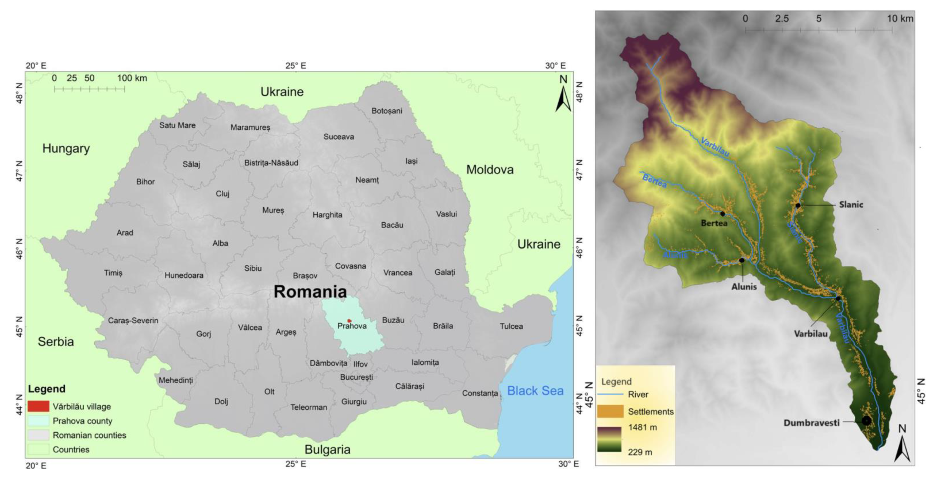
The Vărbilau catchment is situated in Prahova County (Romania) and is a sub-basin of the Teleajen basin, with an altitude between 229 and 1481 m and a surface of 215 km2. The Curvature Carpathians are in its north, while its south and center belong to the SubCarpathians. This position favors an increased amount of precipitation from south to north. The vegetation is diverse due to the existence of mountainous areas, hills, and plains [9]. The basin form is circular in the north and center (Figure 1) and elongated in the south.
Vărbilau River, with a length of 34 km, flows into Teleajen near Dumbrăveşti village. The climate is temperate–continental, which is influenced by local factors, such as the Carpathians, and the opening in the south that communicates with the Romanian plain. The alternation of valleys and hills affects the temperature. It is colder in the north and warmer in the south. Precipitation increases from 600 mm/m2/year in the south to 900 mm/m2/year in the north [7]. The vegetation consists mainly of deciduous forests in hilly zones, pastures, transitional woodland, shrubs, and mixed forests in the north.
In the flat areas, the vegetation was replaced with arable land and settlements [31]. The lithology comprises sedimentary formations, such as flysch in the north, sandstone, clay, sandy–loamy formations, gravel, and marl. The soil patterns influence the infiltration and further percolation in aquifers.
The largest settlement is Vărbilău village, and the closest town is Slănic. In the past, some floods in the area have affected Slănic, Vărbilău, Aluniş, Ştefeşti, and Lutu Roşu [32].
2.2. Methodology
In this article, the flood susceptibility of the study area was evaluated through a Flood Potential Index defined as follows:
where n is the number of themes, m is the number of classes for a theme, is the jth thematic layer’s weight, is the jth class weight from the ith layer [33].
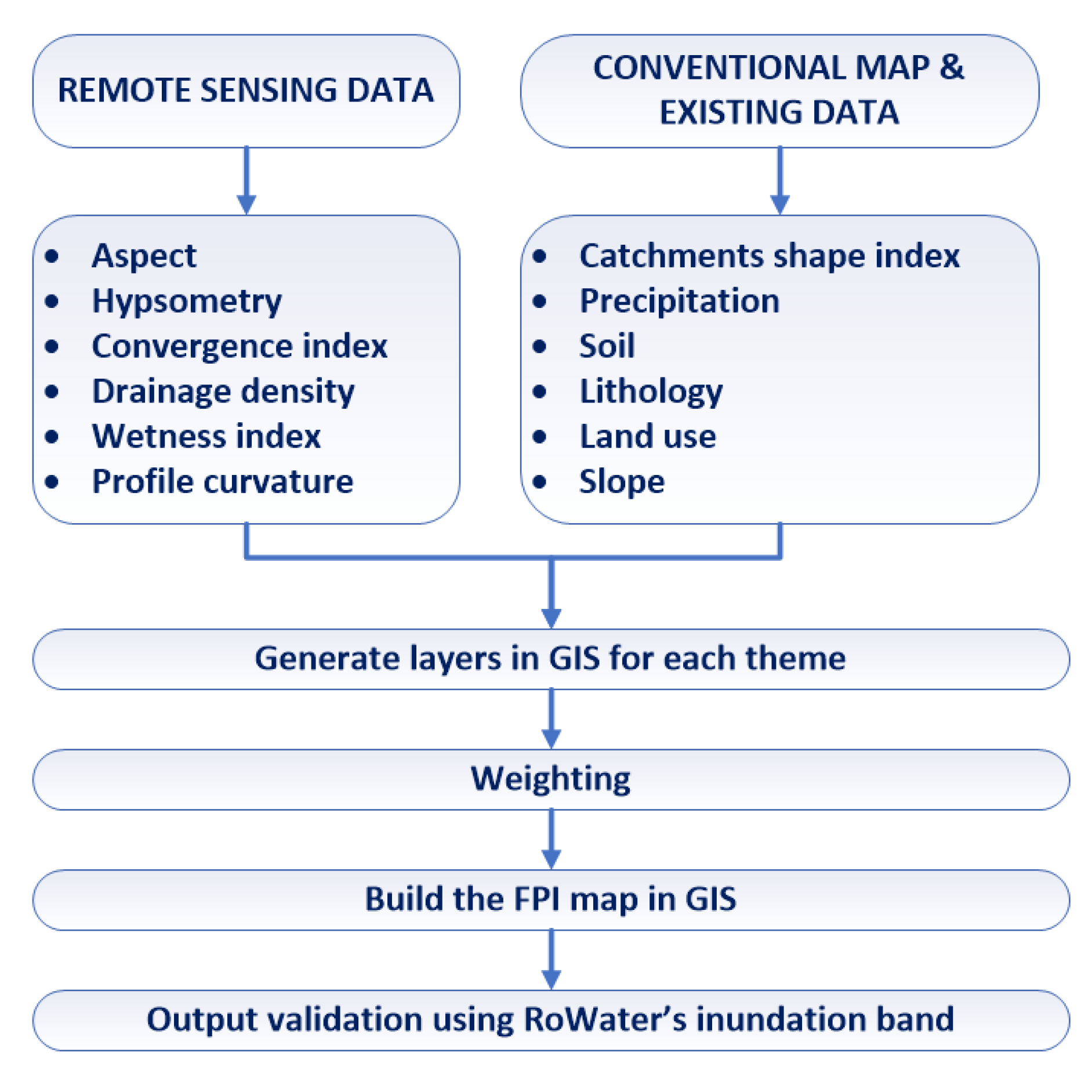
The study’s flow chart is presented in Figure 2, and the proposed methodology steps are described in the following passage.
- 1.
- Select the factors (themes) taken into account for building FPI slope (SL), aspect (A), hypsometry (HY), convergence index (CF), drainage density (DD), topographic wetness index (TWI), profile curvature (PC), catchment shape index (CS), precipitation (P), soil (S), lithology (LH), land use (LU), and classes for each (usually five).
- 2.
- Generate the layers for each theme based on the collected data. The software used for this purpose included the GIS applications ArcMap 10.2.2 (https://support.esri.com/en/products/desktop/arcgis-desktop/arcmap/10-2-2, accessed on 13 May 2023) and SagaGIS 8.5.1 (https://saga-gis.sourceforge.io/en/index. html, accessed on 15 May 2023). After processing, the databases utilized in shapefile and raster formats were exported in .jpg format. The precipitation database (raster format) was from Worldclim.com (https://worldclim.com/, accessed on 20 April 2023) for 12 months from 2010 to 2018. The land use data were from the Corine Land Cover database-ESRI FGDB (https://land.copernicus.eu/pan-european/corine-land-cover, accessed on 13 May 2023). The shapefile layers of the soils, lithology, limits of the hydrographic basin, and the main rivers and Digital Elevation Model (DEM) of the Vărbilău basin have also been used [34,35]. The convergence index was obtained from SAGA GIS 8.5.1. The slope and profile curvature were built from ASTER DEM. The DEM is part of the national numerical model of Romania at 30 cm which was individualized at the hydrographic basin level, in the case of the Vărbilău face. The resolution of the DEM per pixel is 30 m, which is sufficient for what we need in the development of the index in a hydrographic basin, this being already specified;
- 3.
- Compute the drainage density layers in ArcGIS;
- 4.
- Assign the thematic layers’ weights using the multi-criteria decision-making (MCDM) introduced by Saaty [36], as follows:
- Build the comparison matrix of the pairs of themes and assign a score as a function of the relative importance of a theme with respect to another one;
- Normalize the scores by dividing each score through the corresponding column’s sum in the comparison matrix;
- Build the weights vector containing the averages of the rows’ normalized scores.
- 5.
- Validate the weighting choice by computing the following values:
- The maximum eigenvector of the comparison matrix, ;
- The consistency index as follows:
- c.
- The consistency ratio (CR) as follows:
The pair-wise comparison must be reevaluated if CR > 0.1.
- 6.
- Divide the values of each thematic layer into five classes (depending on the importance of its feature in the flood occurrence) and assign a score from 1 to 5 to each class;
- 7.
- Build the FPI map in GIS by integrating the elements from the second step with the weight from step 3;
- 8.
- Compare the results with those obtained when assigning equal weights (8.33%) to each layer;
- 9.
- Validate the model using the flooding simulation maps from RoWater [37], which were realized by experts in hydrology from technical universities in Romania and the Romanian Water Institute in the following stages: developing the digital terrain model (DEM); image processing for the DEMs included in the analysis; hydraulic modeling (including the model calibration) using an exceedance probability of 1%, emphasizing the flood band resulted after hydraulic modeling (to observe the flood impact on settlements and land); intersecting areas of interest with flood band based on road, rail, settlement, industrial, land use, forest, etc. database.
We did not consider it necessary to repeat all the hydraulic simulations here for the entire Vărbilău basin.
3. Results and Discussion
Table 1 contains the factors considered in modeling, their classes, and the scores assigned to each class.
The slope represents the inclination of a surface with respect to the horizontal. A large slope favors water leakage and erosion, while a small one results in water accumulation. Therefore, score five was given to slopes between 0 and 5.36 degrees, and score 1 was given to slopes from 22.65 to 44.1 degrees (Table 1).
The slope was derived from the DEM using the “Slope” extension from the Raster Surface tool in ArcMap. The resulting index is in raster format. In Figure 3 (left), one may see the spatial representation of the slope.
The aspect is the slope’s orientation. Its influence is indirect because it impacts the soil humidity, evapotranspiration, and the frontal rainfall direction [38]. It was determined based on the DEM using “Aspect” from the Raster Surface extension in ArcMap. Figure 3 (right) presents the slope orientations. Those located towards the NW, N, and NE received a value of three because the northern slopes are more shaded than the southern ones. For example, the snow melts slower in these areas. The western and eastern aspects were given a value of four, while the flat areas and the slopes oriented towards the SW, S, and SE were given a five because they either favor water accumulation (in the case of flat land) or snow melting (in the case of those oriented towards the south).
Hypsometry shows the altitudes in the Vărbilău basin. Low-lying areas favor flooding, and thus received high values. In Figure 4 (left), the spatial representation of hypsometry can be observed.
The convergence index indicates the relief structure as a collection of convergent and divergent zones [39], that is, the mean difference “between real aspect and theoretical maximum divergent direction matrix representing ideal peak minus 90 degrees” [40]. Generally, high values of the index indicate the possible apparition of torrential water flows [39,41].
The convergence index was created in SagaGIS and exported as a DEM to be imported into ArcGIS. Values below (−9.6) were given a value of 5, while those above (−3.2) were given a 3, the latter favoring the accumulation of water the least. Figure 4 (right) shows the spatial representation of the convergence index.
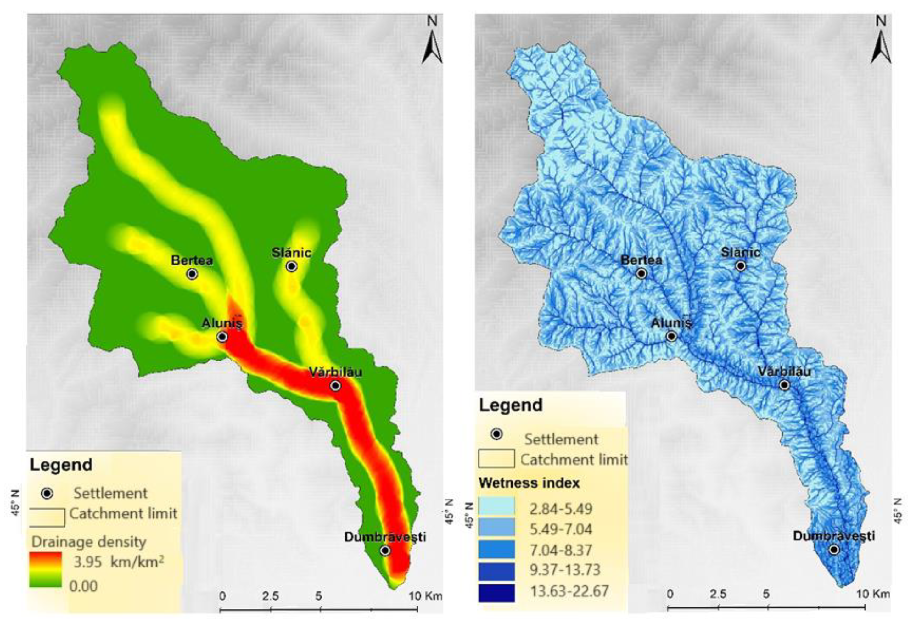
The drainage density was obtained using several tools from Spatial Analyst in ArcGIS. It was determined based on the line density, equivalent to the river valleys. After a tributary meets the main collector, the drainage density is higher. Thus, the density is higher downstream of the Vărbilău catchment (Figure 5 (left)). The higher the density, the higher the value awarded is.
The topographic wetness index is defined as follows:
TWI = log(SCA/tan(b)),
The TWI was built in ArcMap based on the DEM, using the tools from Spatial Analyst in the following order: hydrology extension (“Fill”, “Flow direction”, “Flow accumulation”, “Slope in degrees”), then surface (“Slope”), and finally “Radians of slope”. Figure 5 (right) shows the wetness index. The higher this index is, the higher the grade awarded [43]. The highest drainage density and TWI were found along the river, from Aluniș to Vărbilau and Dumbrăvești villages.
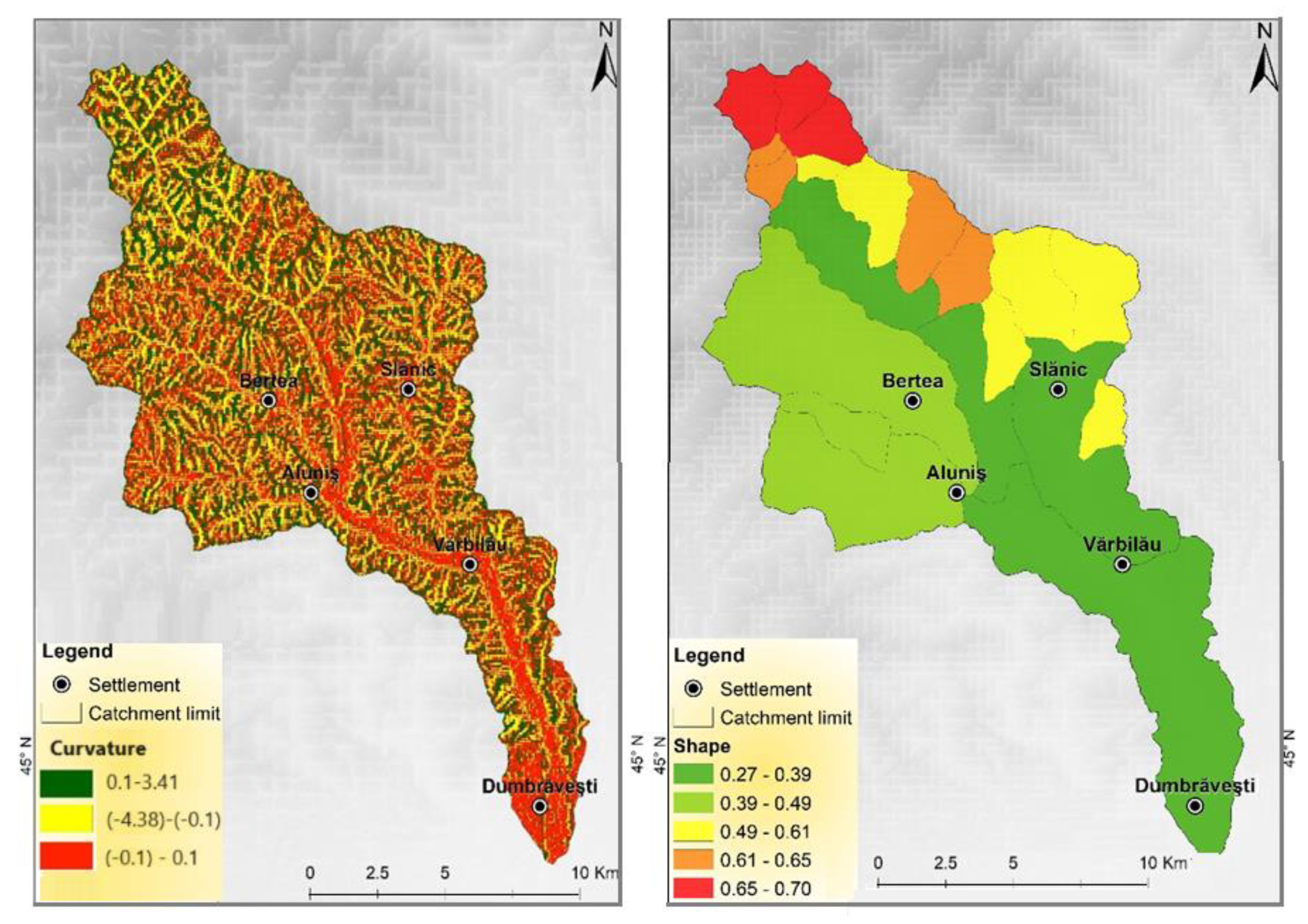
The profile curvature (Figure 6 (left)) was obtained based on the DEM in ArcGIS (raster surface). A negative value means that a surface is upward convex at a cell. A positive profile indicates that a surface is upward concave at a cell. A value of zero indicates that the surface is flat.
Thus, the flat areas have been given the highest score of 5; values from 0.1 to 3.41 were awarded 3, whereas the ones from (−0.1) to (−4.38) have been given 1. Figure 6 (left) shows an alternation of the highest and moderate curvature, especially in the northern part of the river basin.
The catchment shape index was calculated in ArcMap, after the sub-basins were delimited (Figure 6 (right)) using the following formula:
where F is the basin’s surface and L is its length.
CS = F/L2,
The basins with elongated shapes favor water accumulation, so they had a higher index value [31]. This was the case for the sub-basin represented with green in Figure 6 (right), to which Slănic, Vărbilău, and Dumbrăveni belong.
The precipitation map was obtained in ArcGIS as a raster (Figure 7 (left)). First, the yearly precipitation was calculated using the “Raster Calculator” (all 12 months were cumulated for each year).
Then, the annual average was computed. For the Vărbilău catchment, the precipitation increased from south to north, from 600 to 900 mm/m3/year. The areas with low rainfall received a score of 3, while the ones in the north with higher values received a 5.
The soil theme is represented in Figure 7 (right). The predominant soils are clayey-sandy soils (in the northern part of the study basin and in the vicinity of Aluniș and Vărbilău villages), clays, and limy sandstones. Based on the soil texture, different marks were awarded. For example, loamy soils received a 5, while sandy–loamy soils received a 1 because water infiltrates through them faster [44].
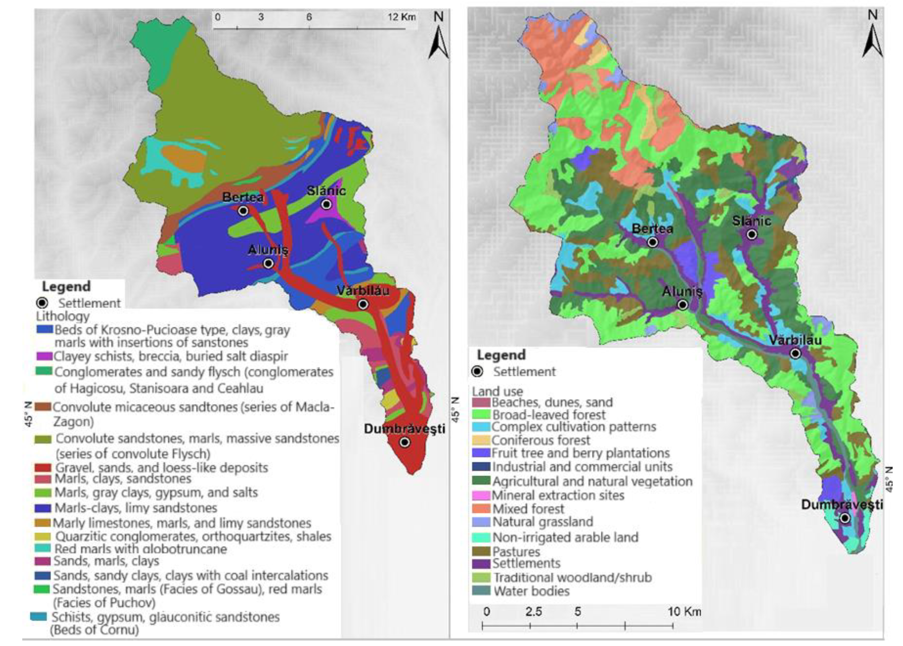
The lithology map is shown in Figure 8 (left). Convolute sandstones, marls, and massive sandstones, conglomerates of sandy flysch, dominate the north of the basin (covering more than a third of the region).
Marls–clay and limy stones are found in the middle of the region, while in the zones along the river and in the southern part, gravels, sands, and loess-like deposits are preponderant.
Water can pass quickly through sandy soils (which are permeable), so the runoff is reduced. By comparison, clay has a more negligible permeability; the runoff is higher than for sandy soils, and, as a consequence, water accumulates for an increased period. Therefore, flood risk is inversely proportional to the infiltration capacity.
According to the lithology influence on water accumulation, grades were awarded from one for gravels, sands, and loess-like deposits, to five for conglomerates and sandy flysch [45,46].
The land use map (Figure 8 (right)) was obtained in ArcMap based on the data from Corine Land Cover. Vegetation impacts the soil’s capacity to diminish runoff. Therefore, forest areas received a score of 1 because they have a role in retaining water in the upper parts. In contrast, settlements, water bodies, and industrial or commercial units received five because they favor water accumulation [46].
Furthermore, to obtain the Flood Potential Index, the factors that were represented in shapefiles (land use, lithology, soil, catchment shape) in ArcMap were converted into raster format.
Afterwards, with the help of the “Raster Calculator,” the twelve factors were cumulated to obtain the FPI [47] in two scenarios: (I) with the weights computed as explained in the Methodology or (II) with equal weights (8.33%).
Table 2 contains the comparison matrix. Based on the computed weights (in the last column) and the thematic maps, the FPI index was determined.
The obtained values were split into five intervals based on the ‘natural breaks’ [48] idea because differences between the classes are maximized whereas those inside them are minimized. The following classes were obtained based on the FPI values: very low vulnerability, when FPI is in the interval 2.04–2.65; low vulnerability, with an FPI between 2.65 and 3.02; medium vulnerability, with an FPI from 3.02 to 3.34; high vulnerability, with an FPI from 3.34 to 3.68; and very high vulnerability, with an FPI between 3.68 and 4.50.
Figure 9 shows the susceptibility map in the first scenario (unequal weights), with and without intervals, which is discussed in the following section. The Vărbilău basin registers a greater susceptibility along its lower and middle course (3.68–4.50), at the confluences of the Slănic and Vărbilău rivers and the Aluniş and Bertea rivers, and in the area of the Slănic town, on the river with the same name. Moreover, the most extended regions with very high susceptibility (3.68–4.50) were located in Varbilău, Ostrovu, Slănic, and Dumbrăveşti. The factors that make these areas susceptible are, among others, the elongated shape of the basins, the almost flat slope, the humidity index, and the land use (inhabited areas favor floods) [49,50].
In general, areas with a high susceptibility to flooding were identified in the valleys. In hilly zones, the vulnerability was average (3.02–3.34). There, the values of the slope index were medium, along with the hypsometric and soil values. Furthermore, the population density is low. Low flood susceptibility values were found in mountainous areas with steep slopes. The sub-basin shape in mountainous area was circular, so water accumulation is low. One may observe that the areas with high population densities (Slănic, Ostrovu, Aluniș, Dumbrăvești, Târșoreni, Scurtești, Poiana Vărbilău) showed a high (3.34–3.68) and very high (3.68–4.50) susceptibility to floods.
Figure 10 presents a comparison of the obtained FPIs with different (left) and equal weights (right). In the case of equal weights, a smaller surface of the basin belongs to the high susceptibility class, most of it being in the low and medium susceptibility classes.
The difference appears because the importance of some factors (precipitation, slope, hypsometry) is diminished in the second case. Therefore, a good selection of weights is necessary. Figure 11 and Figure 12 contain a zoomed-in view of two areas with a high and very high susceptibility to flooding. The Aluniş–Ostrovu area (Figure 11 (left) and Figure 12 (left)) is located at a confluence. The Strâmba River flows into Aluniş, which, after a few hundred meters, flows into Bertea.
The Bertea River, which borders the village of Ostrovu to the west, flows into Vărbilău in the southern part of the same village. Here, there are three confluences in less than 1.5 km. With a high population density, this area is among the most susceptible to floods. Aluniş village was heavily affected by flooding in 2019. The Vărbilău commune (Figure 11 and Figure 12 (right)) has been affected by flooding many times.
Comparisons of Figure 11 and Figure 12 show the importance of the weight selection, revealed by the areas of high and very high susceptibility to flooding with a lower extent in the second scenario.
The buildings that overlap the area with high susceptibility can be observed in Figure 13 (left).
Notice that a significant number of settlements are prone to flooding based on the susceptibility index.
Data from the Romanian Waters Institute, including flood zone maps, at an exceedance probability of 1%, were utilized to validate the results obtained using the FPI approach. These were superimposed on the highest susceptibility index (3.68–4.50). Figure 13 (right) shows that the Vărbilău River’s inundation band (in blue) largely overlaps the area where the estimated flood susceptibility is very high.
The present study completes the simulation provided by RoWater [34], developing an FPI index that shows the areas that are also susceptible to flooding and could be affected in the future by the hazard.
The FPI index is an indicator developed using several factors that have been calculated or determined based on field observation, a digital terrain model, or other supporting values. The obtained FPI is unique for the area of study that does not have a detailed susceptibility index map.
4. Conclusions
The Flood Potential Index obtained using ArcGIS can be used to assess the hydrological impact in a given area, separately or together with other analyses, especially in the context of the recurrence of hydrologic phenomena such as floods. Depending on the area’s specifics, it can also be spatially represented and analyzed in detail at the constituent factor level. Other factors can be introduced for building the index, which can be adapted to the user’s needs.
The proposed methodology can be used for any region by adapting the factors to the catchment particularities. In the second scenario, the importance of the factors was established based on the scientific literature and a deep knowledge of the field situation. Still, the user’s experience also influences the weight selection when FPI is computed. It was proved that when using weights, the FPI better described the vulnerable areas.
It was shown that in the Vărbilău basin, the densely populated areas have a high and very high susceptibility to flooding. In contrast, uninhabited mountain areas present a very low susceptibility. Settlements such as Vărbilău, Aluniş, Ostrovu, Bertea, Slănic, and Dumbrăveşti have a high susceptibility to floods as a result of the flat land, the elongated shape of the basin, the presence of settlements, and the absence of forests.
This study represents part of a bigger project aiming to quantify the hazard risk and accessibility in the region in the case of extreme events and to evaluate damage. It will help the authorities make informed decisions to prevent or reduce the effects of possible flooding in the study zone.
Author Contributions
Conceptualization, N.-C.P. and A.B.; methodology, N.-C.P. and A.B.; software, N.-C.P.; validation, N.-C.P. and A.B.; formal analysis, A.B.; investigation, N.-C.P. and A.B.; resources, N.-C.P. and A.B.; data curation, N.-C.P.; writing—original draft preparation, N.-C.P. and A.B.; writing—review and editing, A.B.; visualization, N.-C.P.; supervision, A.B.; project administration, A.B.; funding acquisition, N.-C.P. All authors have read and agreed to the published version of the manuscript.
Funding
The publication fee was supported for the first author by the Technical University of Civil Engineering of Bucharest, Romania.
Data Availability Statement
Data will be available on request.
Conflicts of Interest
The authors declare no conflict of interest.
References
- McPhillips, L.E.; Chang, H.; Chester, M.V.; Depietri, Y. Defining Extreme Events: A Cross-Disciplinary Review. Earth’s Future 2018, 6, 441–455. [Google Scholar] [CrossRef]
- Chang, S.E.; Gregorian, M.; Pathman, K.; Yumagulova, L.; Tse, W. Urban growth and long-term changes in natural hazard risk. Environ. Plann. A 2012, 44, 989–1008. [Google Scholar] [CrossRef]
- United Nations Office for Disaster Risk Reduction. Global Assessment Report on Disaster Risk Reduction. 2013. Available online: https://www.undrr.org/publication/global-assessment-report-disaster-risk-reduction-2013 (accessed on 6 March 2023).
- Visser, H.; Petersen, A.C.; Ligtvoet, W. On the relation between weather-related disaster impacts, vulnerability and climate change. Clim. Change 2012, 125, 461–477. [Google Scholar] [CrossRef]
- Gill, J.C.; Malamud, B.D. Reviewing and visualizing the interactions of natural hazards. Rev. Geophys. 2014, 52, 680–722. [Google Scholar] [CrossRef]
- Thodsen, H.; Baattrup-Pedersen, A.; Andersen, H.E.; Brask Jensen, K.M.; Mejlhede Andersen, P.; Bolding, K.; Ovesen, N.B. Climate change effects on lowland stream flood regimes and riparian rich fen vegetation communities in Denmark. Hydrol. Sci. J. 2016, 91, 344–358. [Google Scholar] [CrossRef]
- Ciulache, S.; Ionac, N. Essential in Meteorology and Climatology; Editura Universitară: Bucharest, Romania, 2007. (In Romanian) [Google Scholar]
- Gaume, E.; Bain, V.; Bernardara, P.; Newinger, O.; Barbuc, M.; Bateman, A.; Blaškovičová, L.; Blöschl, G.; Borga, M.; Dumitrescu, A.; et al. A compilation of data on European flash floods. J. Hydrol. 2009, 367, 70–78. [Google Scholar] [CrossRef]
- Askar, S.; Zeraat Peyma, S.; Yousef, M.M.; Prodanova, N.A.; Muda, I.; Elsahabi, M.; Hatamiafkoueieh, J. Flood Susceptibility Mapping Using Remote Sensing and Integration of Decision Table Classifier and Metaheuristic Algorithms. Water 2022, 14, 3062. [Google Scholar] [CrossRef]
- Pandey, M.; Arora, A.; Arabameri, A.; Costache, R.; Kumar, N.; Mishra, V.N.; Nguyen, H.; Mishra, J.; Siddiqui, M.A.; Ray, Y.; et al. Flood Susceptibility Modeling in a Subtropical Humid Low-Relief Alluvial Plain Environment: Application of Novel Ensemble Machine Learning Approach. Front. Earth Sci. 2021, 9, 659296. [Google Scholar] [CrossRef]
- Samanta, S.; Pal, D.K.; Palsamanta, B. Flood susceptibility analysis through remote sensing, GIS and frequency ratio model. Appl. Water Sci. 2018, 8, 66. [Google Scholar] [CrossRef]
- Dottori, F.; Martina, M.L.V.; Figueiredo, R. A methodology for flood susceptibility and vulnerability analysis in complex flood scenarios. J. Flood Risk Manag. 2016, 11, S632–S645. [Google Scholar] [CrossRef]
- Rincón, D.; Khan, U.T.; Armenakis, C. Flood Risk Mapping Using GIS and Multi-Criteria Analysis: A Greater Toronto Area Case Study. Geoscience 2018, 8, 275. [Google Scholar] [CrossRef]
- Sitterson, J.; Knightes, C.; Parmar, R.; Wolfe, K.; Muche, M.; Avant, B. An Overview of Rainfall-Runoff Types. U.S. Environmental Protection Agency, Office of Research and Development. EPA/600/R-14/152, 217. Available online: https://cfpub.epa.gov/si/si_public_record_report.cfm?dirEntryId=339328&Lab=NERL (accessed on 7 October 2023).
- England, J.F.; Cohn, T.A.; Faber, B.A.; Stedinger, J.R.; Thomas, W.O.; Veilleux, A.G.; Kiang, J.E.; Mason, R.R. Guidelines for Determining Flood Flow Frequency. Bull. 17C. U.S. Department of Interior, U.S. Geological Survey, Techniques and Methods 4-B5. 2018. Available online: https://pubs.usgs.gov/tm/04/b05/tm4b5.pdf (accessed on 7 October 2023).
- Yochum, S.E.; Scott, J.A.; Levinson, D.H. Methods for Assessing Expected Flood Potential and Variability: Southern Rocky Mountains Region. Water Resour. Resear. 2019, 55, 6392–6416. [Google Scholar] [CrossRef]
- Bellos, V. Ways for flood hazard mapping in urbanised environments: A short literature review. Water Util. J. 2012, 4, 25–31. [Google Scholar]
- Di Baldassarre, G.; Montanari, A.; Lins, H.; Koutsoyiannis, D.; Brandimarte, L.; Blöschl, G. Flood fatalities in Africa: From diagnosis to mitigation. Geophys. Res. Lett. 2010, 37, L22402. [Google Scholar] [CrossRef]
- Pham, B.T.; Avand, M.; Janizadeh, S.; Van Phong, T.; Al-Ansari, N.; Ho, L.S.; Das, S.; Van Le, H.; Amini, A.; Bozchaloei, S.K. GIS based hybrid computational approaches for flash flood susceptibility assessment. Water 2020, 12, 683. [Google Scholar] [CrossRef]
- Al-Juaidi, A.E.; Nassar, A.M.; Al-Juaidi, O.E. Evaluation of flood susceptibility mapping using logistic regression and GIS conditioning factors. Arab. J. Geosci. 2018, 11, 765. [Google Scholar] [CrossRef]
- Hong, Y.; Abdelkareem, M. Integration of remote sensing and a GIS-based method for revealing prone areas to flood hazards and predicting optimum areas of groundwater resources. Arab. J. Geosci 2022, 15, 114. [Google Scholar] [CrossRef]
- Alarifi, S.S.; Abdelkareem, M.; Abdalla, F.; Alotaibi, M. Flash Flood Hazard Mapping Using Remote Sensing and GIS Techniques in Southwestern Saudi Arabia. Sustainability 2022, 14, 14145. [Google Scholar] [CrossRef]
- Abrams, M.; Yamaguchi, Y.; Crippen, R. Aster Global Dem (GDEM) Version 3. Int. Arch. Photogramm. Remote Sens. Spatial Inf. Sci. 2022, XLIII-B4-2022, 593–598. [Google Scholar] [CrossRef]
- Albano, R.; Mancusi, L.; Sole, A.; Adamowski, J. FloodRisk, A collaborative free and open-source software for flood risk analysis. Geomat. Nat. Hazards Risk 2017, 8, 1812–1832. [Google Scholar] [CrossRef]
- Smith, G. Flash Flood Potential: Determining the Hydrologic Response of ffmp Basins to Heavy Rain by Analyzing Their Physiographic Characteristics. 2003. Available online: https://www.cbrfc.noaa.gov/papers/ffpwpap.pdf (accessed on 27 January 2023).
- Costache, R.; Zaharia, L. Flash-flood potential assessment and mapping by integrating the weights-of-evidence and frequency ratio statistical methods in GIS environment—Case study: Bâsca Chiojdului River catchment (Romania). J. Earth Syst. Sci. 2017, 126, 59. [Google Scholar] [CrossRef]
- Usman Kaoje, I.; Abdul Rahman, M.Z.; Idris, N.H.; Razak, K.A.; Wan Mohd Rani, W.N.M.; Tam, T.H.; Mohd Salleh, M.R. Physical Flood Vulnerability Assessment using Geospatial Indicator-Based Approach and Participatory Analytical Hierarchy Process: A Case Study in Kota Bharu, Malaysia. Water 2021, 13, 1786. [Google Scholar] [CrossRef]
- Ţîncu, R.; Zêzere, J.L.; Lazar, G. Identification of elements exposed to flood hazard in a section of Trotus River, Romania. Geomat. Nat. Hazards Risk 2018, 9, 950–969. [Google Scholar] [CrossRef]
- Popa, M.C.; Peptenatu, D.; Drăghici, C.C.; Diaconu, D.C. Flood Hazard Mapping Using the Flood and Flash-Flood Potential Index in the Buzău River Catchment, Romania. Water 2019, 11, 2116. [Google Scholar] [CrossRef]
- Ielenicz, M. Physical Geography of Romania, Volume II—Climate, Waters, Vegetation, Soils, Environment; Editura Universitară: Bucharest, Romania, 2007. (In Romanian) [Google Scholar]
- Velcea, V.; Savu, A. Geography of the Romanian Carpathians and Subcarpathians; Editura Didactică şi Pedagogică: Bucharest, Romania, 1982. (In Romanian) [Google Scholar]
- Ghinea, D. Geographical Encyclopaedia of Romania; Editura Enciclopedică: Bucharest, Romania, 2000. (In Romanian) [Google Scholar]
- Rejith, R.G.; Anirudhan, S.; Sundararajan, M. Delineation of Groundwater Potential Zones in Hard Rock Terrain Using Integrated Remote Sensing, GIS, and MCDM Techniques: A Case Study from Vamanapuram River Basin, Kerala, India. In GIS and Geostatistical Techniques for Groundwater Science; Venkatramanan, S., Prasanna, M.V., Chung, S.Y., Eds.; Elsevier: Amsterdam, The Netherlands, 2009. [Google Scholar] [CrossRef]
- Prăvălie, R.; Costache, R. The analysis of the susceptibility of the flash-floods genesis in the area of the hydrographical basin of Basca Chiojdului river. Forum Geogr. 2014, XIII, 39–49. [Google Scholar] [CrossRef]
- Zaharia, L.; Minea, G.; Toroimac, I.; Barbu, R.; Sârbu, I. Estimation of the Areas with Accelerated Surface Runoff in the Upper Prahova Watershed (Romanian Carpathians); BALWOIS: Ohrid, North Macedonia, 2012; Available online: https://www.academia.edu/3280129/Estimation_of_the_Areas_with_Accelerated_Surface_Runoff_in_the_Upper_Prahova_Watershed_Romanian_Carpathians (accessed on 23 January 2023).
- Saaty, T.L. The Analytic Hierarchy Process: Planning, Priority Setting, Resource Allocation; McGraw-Hill: New York, NY, USA, 1980. [Google Scholar]
- Hazard and Flood Risk Map (1st Cycle). Available online: https://inundatii.ro/portal-harti/ (accessed on 12 January 2023). (In Romanian).
- Jade, S.; Sarkar, S. Statistical model for slope instability classification. Eng. Geol. 1993, 36, 71–98. [Google Scholar] [CrossRef]
- Kiss, R. Determination of Drainage Network in Digital Elevation Models, Utilities and Limitations. J. Hung. Geomath. 2004, 2, 16–29. [Google Scholar]
- ***. Available online: https://grass.osgeo.org/grass82/manuals/addons/r.convergence.html (accessed on 12 January 2023).
- Ramesh, V.; Iqbal, S.S. Urban flood susceptibility zonation mapping using evidential belief function, frequency ratio, and fuzzy gamma operator models in GIS: A case study of Greater Mumbai, Maharashtra, India. Geocarto Int. 2022, 37, 581–606. [Google Scholar] [CrossRef]
- Sørensen, R.; Zinko, U.; Seibert, J. On the calculation of the topographic wetness index: Evaluation of different methods based on field observations. Hydrol. Earth Syst. Sci. 2006, 10, 101–112. [Google Scholar] [CrossRef]
- Kopecky, M.; Macek, M.; Wild, J. Topographic Wetness Index calculation guidelines based on measured soil moisture and plant species composition. Sci. Total Environ. 2021, 757, 143785. [Google Scholar] [CrossRef]
- Patel, K.F.; Fansler, S.J.; Campbell, T.P.; Bond-Lamberty, B.; Peyton-Smith, A.; Chowdhury, T.R.; McCue, L.A.; Varga, T.; Bailey, V.L. Soil texture and environmental conditions influence the biogeochemical responses of soils to drought and flooding. Commun. Earth Environ. 2021, 2, 127. [Google Scholar] [CrossRef]
- Sugianto, S.; Deli, A.; Miswar, E.; Rusdi, M.; Irham, M. The Effect of Land Use and Land Cover Changes on Flood Occurrence in Teunom Watershed, Aceh Jaya. Land 2022, 11, 1271. [Google Scholar] [CrossRef]
- Zhang, G.; Feng, G.; Li, X.; Xie, C.; Pi, X. Flood Effect on Groundwater Recharge on a Typical Silt Loam Soil. Water 2017, 9, 523. [Google Scholar] [CrossRef]
- Costache, R.; Prăvălie, R.; Mitof, I.; Popescu, C. Flood vulnerability assessment in the low sector of Sărăţel catchment. Case study: Joseni village. Carpath. J. Earth Environ. Sci. 2015, 10, 161–169. [Google Scholar]
- Data Classification Methods. Available online: https://pro.arcgis.com/en/pro-app/latest/help/mapping/layer-properties/data-classification-methods.htm (accessed on 20 January 2023).
- Jacinto, R.; Grosso, N.; Reis, E.; Dias, L.; Santos, F.D.; Garrett, P. Continental Portuguese Territory Flood Susceptibility Index—Contribution to a vulnerability index. Nat. Hazards Earth Syst. Sci. 2015, 15, 1907–1919. [Google Scholar] [CrossRef]
- Tehrany, M.S.; Pradhan, B.; Jebur, M.N. Flood susceptibility mapping using a novel ensemble weights-of-evidence and support vector machine models in GIS. J. Hydrol. 2014, 512, 332–343. [Google Scholar] [CrossRef]
Figure 1.
(Left) The location of Prahova County in Romania, and (right) the Vărbilău catchment in Prahova County.
Figure 1.
(Left) The location of Prahova County in Romania, and (right) the Vărbilău catchment in Prahova County.

Figure 2.
The study flowchart.

Figure 3.
The maps of slope (left) and aspect (right).

Figure 4.
Hypsometry (left) and convergence index (right).

Figure 5.
Drainage density (left) and TWI (right).

Figure 6.
Profile curvature (left) and catchment shape (right) maps.

Figure 7.
The maps for precipitation (left) and soil (right).

Figure 8.
Lithology (left) and land use (right) maps.

Figure 9.
FPI with unequal weights with (left) and without (right) intervals.

Figure 10.
FPI with unequal weights (left) and equal weights (right).

Figure 11.
Zoomed-in areas with high susceptibility: Aluniş–Ostrovu (left) and Vărbilău (right), under the scenario with different weights.
Figure 11.
Zoomed-in areas with high susceptibility: Aluniş–Ostrovu (left) and Vărbilău (right), under the scenario with different weights.

Figure 12.
Zoomed-in areas with high susceptibility: Aluniş–Ostrovu (left) and Vărbilău (right), under the scenario with equal weights.
Figure 12.
Zoomed-in areas with high susceptibility: Aluniş–Ostrovu (left) and Vărbilău (right), under the scenario with equal weights.

Figure 13.
Areas with very high susceptibility (left) and flooding surfaces and susceptibility index comparison (right).
Figure 13.
Areas with very high susceptibility (left) and flooding surfaces and susceptibility index comparison (right).


Table 1.
The scores of the factors influencing the flood potential.
| Factors | Type/Values | ||||
|---|---|---|---|---|---|
| Slope (degrees) | 22.65–44.1 | 15.39–22.65 | 10.37–15.39 | 5.36–10.37 | 0–5.36 |
| Aspect | N, NW, NE | W, E | Flat, S, SW, SE | ||
| Hypsometry (m) | 1079–1481 | 818–1079 | 606–818 | 430–606 | 229–430 |
| Convergence index | >(−3.2) | (−9.6)–(−3.2) | <−9.6 | ||
| Drainage density (km/km2) | 0–0.79 | 0.79–1.58 | 1.58–2.37 | 2.37–3.16 | 3.16–3.95 |
| TWI | 2.84–5.49 | 5.49–7.04 | 7.04–9.37 | 9.37–13.73 | 13.73–22.67 |
| Profile curvature (radians/m) | 0.1–3.41 | (−4.38)–(−0.1) | (−0.1)–0.1 | ||
| Catchment shape index | 0.65–0.70 | 0.61–0.65 | 0.49–0.61 | 0.39–0.49 | 0.27–0.39 |
| Precipitation (mm/year) | 600–700 | 700–800 | 800–900 | ||
| Soil | sandy−loamy, loamy−sandy | sandy and loamy | varied textures, clayey, clayey−loamy | loamy−clayey, loamy | loamy |
| Lithology | Gravels, sands and loess−like deposits | Marly limestones, marls, and limy sandstones Marls−clays, limy sandstones Sands, marls, clays | Marls, clays, sandstones, Marls, gray clays, gypsum and salts Beds of Krosno−Pucioasa type; clays, gray marls with insertions of sandstones Red marls with Globotruncana | Clayey schists, breccia, buried salt diaper. Schists, gypsum, glauconitic sandstones (beds of Cornu) Quartzitic conglomerates, orthoquartzites, shales Convolute sandstones, marls, massive sandstones (series of Convolute Flysch) | Conglomerates and sandy flysch (conglomerates of Hacigosu, Stanisoara, and Ceahlau) Convolute micaceous sandstones (series of Macla−Zagon) |
| Land use | Broad-leaved forest Coniferous forest Mixed forest | Fruit trees and berry plantations Transitional woodland/shrub Beaches, dunes, sands | Complex cultivation patterns Land with agriculture and natural vegetation Non-irrigated arable land | Pastures Natural grassland Mineral extraction sites | Settlements Water bodies Industrial or commercial units |
| Given score | 1 | 2 | 3 | 4 | 5 |
| FPI | 2.06−2.65 (very low) | 2.65−3.02 (low) | 3.02−3.34 (medium) | 3.34−3.68 (high) | 3.68−4.50 (very high) |
Table 2.
Comparison matrix of the thematic layers and the weights (in the last column).
| Factor | SL | A | HY | CF | DD | TWI | PC | CS | P | S | LH | LU | Weights |
|---|---|---|---|---|---|---|---|---|---|---|---|---|---|
| SL | 1.00 | 2.00 | 0.50 | 0.50 | 3.00 | 1.00 | 1.00 | 0.25 | 1.00 | 0.33 | 0.33 | 0.50 | 0.055 |
| A | 0.50 | 1.00 | 0.33 | 0.25 | 1.00 | 0.50 | 0.50 | 0.25 | 0.50 | 0.33 | 0.33 | 0.25 | 0.031 |
| HY | 2.00 | 3.00 | 1.00 | 1.00 | 2.00 | 2.00 | 3.00 | 0.50 | 2.00 | 0.50 | 1.00 | 1.00 | 0.098 |
| CF | 2.00 | 4.00 | 1.00 | 1.00 | 3.00 | 3.00 | 2.00 | 0.50 | 2.00 | 1.00 | 0.50 | 0.50 | 0.1 |
| DD | 0.33 | 1.00 | 0.50 | 0.33 | 1.00 | 1.00 | 2.00 | 0.50 | 1.00 | 0.33 | 0.33 | 0.50 | 0.048 |
| TWI | 1.00 | 2.00 | 0.50 | 0.33 | 1.00 | 1.00 | 1.00 | 0.25 | 0.50 | 0.33 | 0.50 | 0.33 | 0.043 |
| Pc | 1.00 | 2.00 | 0.33 | 0.50 | 0.50 | 1.00 | 1.00 | 0.33 | 1.00 | 0.33 | 0.50 | 0.33 | 0.045 |
| CS | 4.00 | 4.00 | 2.00 | 2.00 | 2.00 | 4.00 | 3.00 | 1.00 | 2.00 | 2.00 | 2.00 | 1.00 | 0.16 |
| P | 1.00 | 2.00 | 0.50 | 0.50 | 1.00 | 2.00 | 1.00 | 0.50 | 1.00 | 0.50 | 1.00 | 1.00 | 0.067 |
| S | 3.00 | 3.00 | 2.00 | 1.00 | 3.00 | 3.00 | 3.00 | 0.50 | 2.00 | 1.00 | 1.00 | 1.00 | 0.122 |
| LH | 3.00 | 3.00 | 1.00 | 2.00 | 3.00 | 2.00 | 2.00 | 0.50 | 1.00 | 1.00 | 1.00 | 0.50 | 0.103 |
| LU | 2.00 | 4.00 | 1.00 | 2.00 | 2.00 | 3.00 | 3.00 | 1.00 | 1.00 | 1.00 | 2.00 | 1.00 | 0.126 |
| Sum | 20.83 | 31.00 | 10.66 | 11.41 | 22.50 | 23.50 | 22.50 | 6.08 | 15.00 | 8.65 | 10.49 | 7.91 | 1.00 |
Disclaimer/Publisher’s Note: The statements, opinions and data contained in all publications are solely those of the individual author(s) and contributor(s) and not of MDPI and/or the editor(s). MDPI and/or the editor(s) disclaim responsibility for any injury to people or property resulting from any ideas, methods, instructions or products referred to in the content. |
© 2023 by the authors. Licensee MDPI, Basel, Switzerland. This article is an open access article distributed under the terms and conditions of the Creative Commons Attribution (CC BY) license (https://creativecommons.org/licenses/by/4.0/).
Share and Cite
MDPI and ACS Style
Popescu, N.-C.; Bărbulescu, A. Flood Hazard Evaluation Using a Flood Potential Index. Water 2023, 15, 3533. https://doi.org/10.3390/w15203533
AMA Style
Popescu N-C, Bărbulescu A. Flood Hazard Evaluation Using a Flood Potential Index. Water. 2023; 15(20):3533. https://doi.org/10.3390/w15203533
Chicago/Turabian StylePopescu, Nicolae-Cristian, and Alina Bărbulescu. 2023. "Flood Hazard Evaluation Using a Flood Potential Index" Water 15, no. 20: 3533. https://doi.org/10.3390/w15203533
Note that from the first issue of 2016, this journal uses article numbers instead of page numbers. See further details here.