Modeling Wetland Functions: Is Space-to-Time Substitution of the Perimeter–Area Relationship Appropriate?

Abstract

Wetlands’ morphometric or shape properties, such as their area and perimeter, impact a multitude of ecosystem functions and services. However, current models used to quantify these functions often only use area as an independent variable, as the static area and perimeter of different wetlands have been found to be closely related. The study uses monthly inundation maps, derived from remote sensing data, to assess the temporal covariation of geographically isolated wetlands’ perimeter and surface area. The results show that using static representations of wetlands to evaluate temporal dynamic perimeter–area relationships can introduce significant discrepancies and that these discrepancies can be reduced if evaluations using static data are performed separately for each wetlandscape. This study concludes that models that use implicit area–perimeter relationships based on static wetland representations, as is usually the case, should be applied with caution. Additionally, it suggests that incorporating perimeter–area relationships from temporally dynamic data can improve estimates of wetland functions.

1. Introduction

Wetlands provide a wide range of invaluable ecosystem services, including contaminant buffering [1], flood protection [2,3], biodiversity support [4], and carbon sequestration [5]. Notably, several of these ecosystem services are strongly related to wetlands’ morphometric or shape attributes. For example, the removal rate of contaminants is related to wetlands’ inundation area and perimeter [6,7,8,9,10], the volume of methane emissions is affected by wetlands’ area [11,12,13,14], and the suitability of aquatic habitats for wetland bird communities is influenced by wetlands’ area and perimeter-to-area ratio [15,16,17,18]. Unsurprisingly, the effect of a wetland’s perimeter and area on its functions is a topic of active study. For example, several studies have focused on assessing habitat suitability [19,20,21,22,23,24,25,26,27,28,29,30,31,32] and erosion and water quality [33,34,35,36,37,38,39,40] vis à vis wetlands’ shape attributes.

The effect of a wetland’s perimeter and area on its function is of particular significance for geographically isolated wetlands (GIWs, hereafter). GIWs usually have a relatively small inundation area but higher perimeter length per unit area, characteristics that make them prominent control points for nutrient removal [41] and other biogeochemical processing at the landscape scale [42,43,44]. Even though these wetlands play an important role in modulating downstream water quality, they have been lost at higher rates [45], in part because they are often accorded limited protections [46], although variably so in different parts of the US [47].

Models quantifying wetland functions in relation to wetlands’ morphometric properties oftentimes only use area as an independent variable [7,44,48,49], in part because the static area and perimeter of different wetlands can be closely related [50]. However, it remains unclear if such a relation between static area and perimeter is valid temporally, as the area and perimeter of wetlands vary with time. Addressing this knowledge gap is essential, as a refined understanding of how wetland area and perimeter covary over time could significantly enhance the precision of models used to quantify ecosystem services. To this end, this study sheds light on the dynamic landscape patterns of GIWs. Specifically, we examine the intricate interplay between perimeter and inundation area, employing diverse shape metrics. The results of our investigation provide insights spanning wetlands of varying sizes, diverse wetness conditions, and an array of wetland landscapes. The goal is to unravel the nuanced relationships between wetland dimensions and their functions, paving the way for more accurate predictive models, and optimal designs of constructed and restored wetlands.

2. Materials and Methods

2.1. Metrics Used to Track the Perimeter–Area Covariation

2.1.1. Perimeter–Area (P:A) Ratio

The P:A ratio is a metric often used to capture a water body’s boundary configuration vis à vis its size. Increasing deviation from a perfectly circular shape results in a higher P:A ratio. In other words, an irregularly shaped wetland must be larger than a circular wetland to have the same P:A ratio value. This metric has been used for quantifying the suitability of water bodies to support biotic habitats [51,52] and to assess the potential of wetlands for sequestering contaminants in the boundary ecotone per unit wetland size [42]. A high P:A ratio is typically associated with wetlands that are hydrologically more dynamic and ecologically diverse, such as marshes and swamps. In contrast, a low P:A ratio is usually associated with wetlands that are more stable and less diverse, such as ponds and lakes. The P:A ratio is calculated as:

$$P:Aratio=\frac{P}{A}$$

(1)

where $P$ is the wetland perimeter in m and $A$ is the wetland area in m². The metric has the advantage of simple calculation, intuitive understanding, and representation. As the metric has a dimension of 1/L where L is a length dimension, its magnitude decreases monotonically with increasing area [42].

2.1.2. Shoreline Fractal Dimension

The shoreline fractal dimension (SFD) was originally developed to quantify the degree of irregularity in oceanic coastlines [53,54,55]. Recently, SFD has also been used to characterize wetlandscapes in US [56]. This metric is a measure of the complexity of the shoreline of a wetland, and is calculated using the following equation:

$$P=k{A}^{\frac{D}{2}}$$

(2)

where $k$ is a proportionality factor, and $D$ is the SFD. As the geometric shape changes from a circle to a line, $D$ changes from $D=1$ for a perfect circle with $P=k\sqrt{A}$ to $D=2$ for a line with $P=kA$. A higher SFD indicates a more complex wetland boundary with enhanced twists and indentations. Given that complex shorelines are known to provide more microhabitats, such as different water depths and water flow patterns, a higher SFD is usually considered to favor higher diversity of plant and animal species found in the wetland. Higher SFD for a wetland is also often interpreted to have larger reactive interface length per unit area, thus highlighting the potential for contaminant buffering. For the evaluation of D using static data of the area and perimeter, $D$ is calculated as the slope of the regression line between $\log P$ and $\log A$ of the wetlands under consideration. In order to evaluate the temporal dynamics of $D$, it is computed using the equation $D=2·\log P/\log A$, assuming $k$ as 1, for each time step. Notably, SFD, just like the P:A ratio, is also a scale-dependent metric.

2.1.3. Shoreline Irregularity

The shoreline irregularity (SI) is the ratio of the perimeter of wetland to the perimeter of a circle of the same area [57,58]. The SI is calculated using the following equation:

$$SI=\frac{P}{2\sqrt{\pi A}}$$

(3)

The smallest wetland area in remote sensing data corresponding to a wetland represented by a pixel has an SI of 1.13, while a perfect circle of the same area has an SI of 1. A crenulated wetland will have a larger SI. This metric has been used for evaluating human impacts on wetlands [45] or explaining wetlands’ functions within their landscapes [16,23,26]. Notably, unlike the two other metrics considered above, i.e., P:A ratio and SFD, SI is dimensionless in nature. However, it should be noted that a recent study highlighted that despite the dimensionless nature of this metric, data resolution may still alter its estimates [59].

2.2. Tracking the Dynamics of Perimeter-Area Covariation

To assess the dynamics of the shape attributes of GIWs, the three aforementioned metrics were evaluated for each time instant that the data existed. Next, variations in these metrics in relation to the wetness were assessed. Here, the wetness at a given time was quantified according to the fractional area of the wetland with respect to its maximal extent in the data period. The evaluation was performed separately for wetlands of different size ranges. For all wetlands with their time-averaged area falling within a size range, metrics were averaged for 20 wetness bins (i.e., 0–5%, 5–10%, etc.) to obtain the dynamical relation of shape metric with wetness.

2.3. Assessing the Representativeness of Dynamic Perimeter-Area Covariation Based on Static Wetland Data

To assess the applicability of perimeter–area relationships obtained from static wetland data for defining temporal dynamics of shape metrics, the static shape-based relationship between perimeter and area was first obtained. To this end, the area and perimeter for all wetlands at their respective maximum extent were derived. The reason for using the maximum extent was because it is consistent with the static relations derived using NWI or similar databases in previous studies. Notably, wetlands in NWI are generally developed based on vegetation, soil, and morphological descriptors that often respond to the maximum inundated area extent [56,60]. This is further confirmed by the 1:1 relation between NWI GIWs and the maximum area extent of remote sensing derived wetlands (Figure S1). Using the area and perimeter of the wetlands’ maximum extent based on remote sensing data, instead of evaluating them from static NWI data, also ensured that the methodology can be applied globally.

Once the area and perimeter of each wetland at its maximum extent were established, averages of the perimeter of all wetlands of identical sizes were obtained. The static area–perimeter relationship was then derived as the linear interpolation between each wetland pair ordered based on increasing area. To obtain the predicted perimeter, and consequently the three aforementioned shape metrics, at a given time, the area for that given time was substituted in the static relation. The differences between the predicted and observed perimeter or shape metric magnitude were quantified as percentage discrepancies. These differences were calculated as the ratio of abs(actual shape metric at any given time instant − estimated shape metric using static data relation)/(estimated shape metric using static data relation). Here, abs() indicates the absolute value. The evaluation was performed for each time step. Next, the discrepancies were time averaged.

2.4. Data

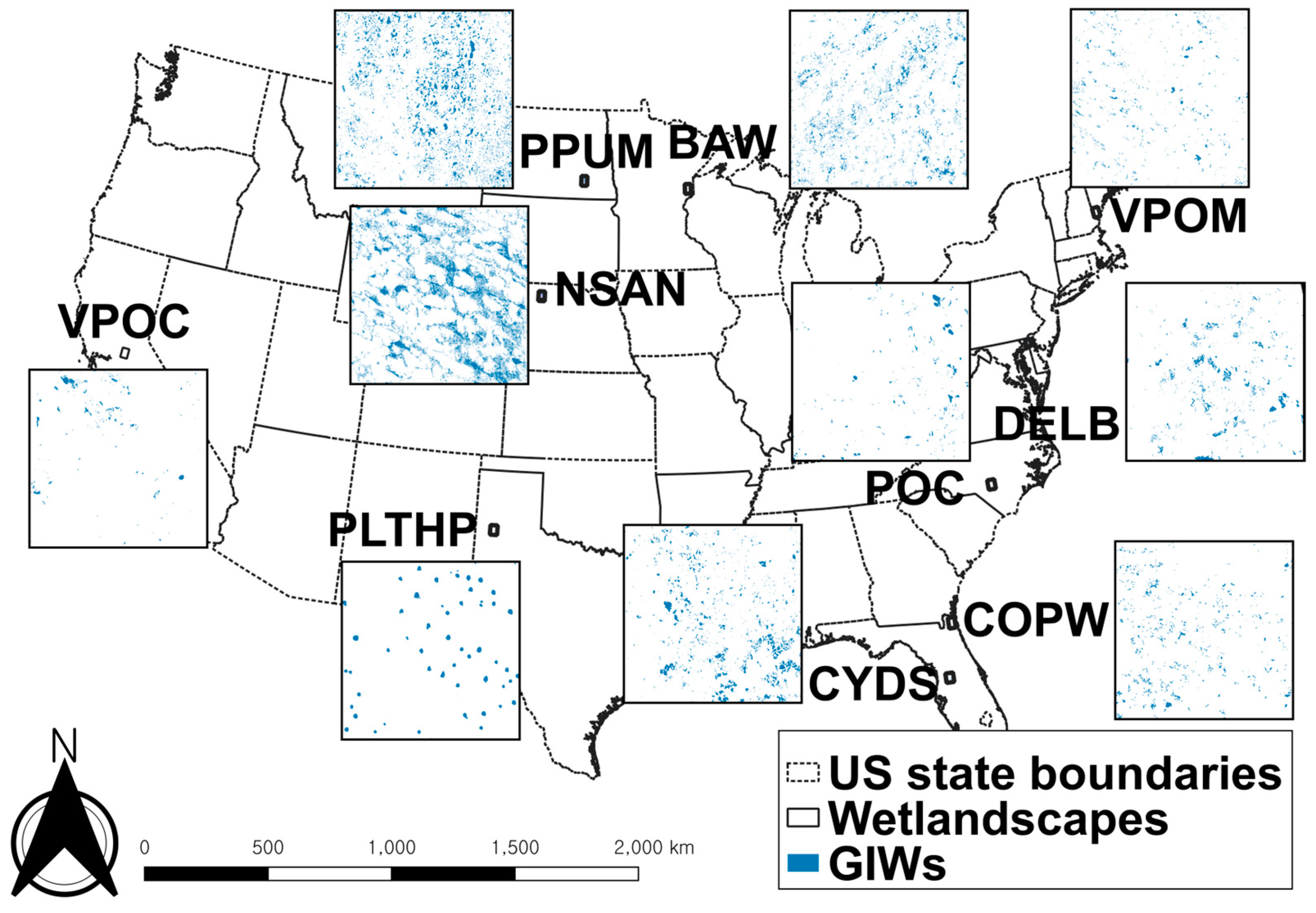
Spatio-temporal variations in wetland extent are usually mapped either by implementing distributed or spatially explicit hydrologic models [61,62,63,64] or post-processing of remote sensing data [65,66,67,68]. For mapping over larger areas (say, at continental scales) at high spatial-resolution, remote sensing data have proven to be particularly effective. For example, the Global Surface Water (GSW) [69] and Dynamic Surface Water Extent (DSWE) [70,71] maps have been used to study inundation dynamics at as fine as 30 m resolution [72,73,74,75] over large areas. Here, we used the monthly inundation maps of GIWs, as derived from remotely sensed data in [75], for ten wetlandscapes in the continental US (Figure 1). Using the GSW v1.0 inundation data from March 1985 to October 2015, the GIWs were derived within 1000 km² area rectangular regions within each wetlandscape. The selected regions were identified to ensure the presence of a sufficient number of wetlands in the study area and the frequent availability of remote sensing data. The method to derive the GIWs in the remotely sensed GSW data followed a two-step process. First, GIWs were identified in the National Wetlands Inventory (NWI) dataset following the rubric presented in [76]. This encompassed several steps including the exclusion of riverine, marine, and estuarine wetlands from ensuing analysis, as they are deemed to have surface connections with water bodies. From among the remaining palustrine and lacustrine wetlands within the study area, we identified the ones that have a higher likelihood of connections with other water bodies during wet periods. To accomplish this, proximity filters were used. Specifically, palustrine and lacustrine wetlands falling within buffer polygons with a radius of 10 m around rivers or lakes with size exceeding 80,000 m², or other water bodies such as reservoirs with area larger than 15,000 m², or water features such as bays/inlets, locks, levees, etc., were excluded. Water polygons from the National Hydrography Dataset (NHD) were used in the analysis. These steps yielded a map of GIWs in the NWI data. Notably, several of these GIWS did not include any wet pixels based on the GSW data. The reason for this discrepancy could be due to inherent uncertainties in these data, or mismatch between the periods when these data were generated. Next, GIWs in the GSW data were identified. To this end, the maximal extent of each wetland in the GSW data was mapped. Then, wetlands that included at least an NWI GIW and also did not touch other non-GIW water bodies in the NWI data were considered as GIWs. The ten wetlandscapes in which GIWs were derived included the Basin wetlands (BAW), Cypress domes of the Southeast (CYDS), Coastal plain wetlands (COPW), Delmarva bays (DELB), Nebraska Sandhills (NSAN), Playa lakes of Texas and High Plains (PLTHP), Prairie potholes of the Upper Midwest (PPUM), Vernal pools of California (VPOC), Vernal pools of Maine (VPOM), and the Pocosins (POC). This study used the derived monthly inundation maps of GIWs to quantify their dynamic shape attributes.

3. Results

3.1. Covariation of Perimeter and Area Based on Static Wetland Data

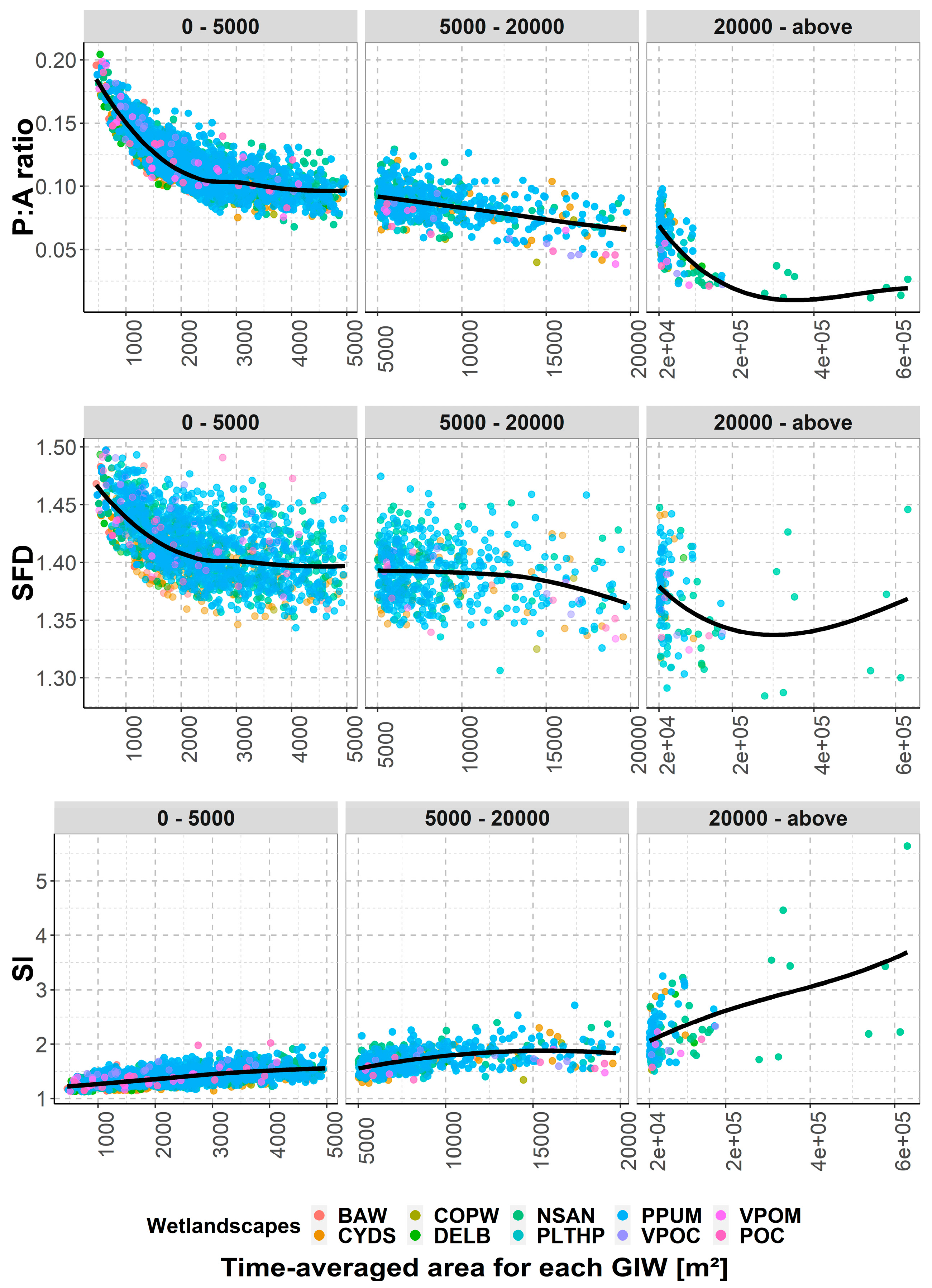
The covariation is evaluated using the best non-linear locally estimated scatterplot smoothing (LOESS) fit line of perimeter–area covariation metrics vis à vis wetland size (Figure 2). While performing this fit, all selected GIWs across the ten wetlandscapes are used. The results show a clear dependence of the P:A ratio, SFD, and SI on wetland size (Figure 2). For larger GIWs, the P:A ratio and SFD generally decrease. This is unsurprising, as both metrics are non-dimensionless, with a length dimension in their denominator, and are expected to decrease with area. The decreasing trend in P:A highlights that with increase in area, there is a proportional but sublinear increase in perimeter. Notably, the two metrics reduce at a faster rate when the wetlands are smaller in size. As SFD is obtained as the ratio of log-transformed perimeter and area, the decrease in it is much smaller than that in the P:A ratio. In contrast to the variations in P:A ratio and SFD, the only dimensionless metric here, i.e., the SI, increases with size. This indicates that larger GIWs have more complex edges or non-rounded shape compared to the smaller GIWs per unit area. It should be acknowledged that for the smallest wetlands with area that encompass only a few pixels (with pixel size = 30 $\times$ 30 m), SI could be uncharacteristically small, as the perimeter representation will likely be much smoother than reality. The aforementioned trends in the considered metrics’ in relation to wetland size are similar regardless of the wetlandscape under consideration (Figure S2), even though the wetlandscapes belonged to diverse hydroclimatic settings [75].

3.2. Dynamic Covariation of Perimeter and Area

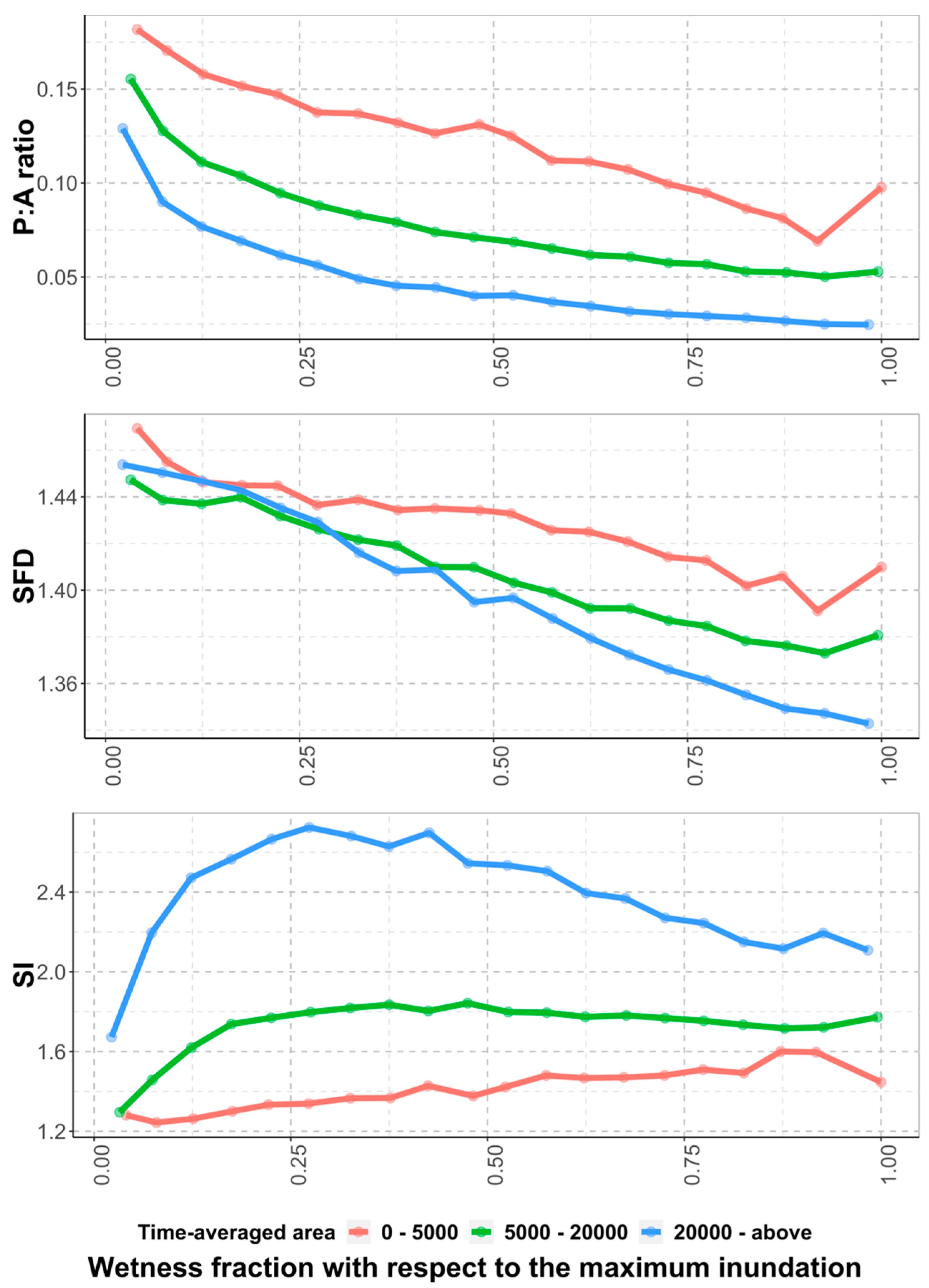
Variation of the P vs. A relationship with time is tracked by evaluating the three metrics as a function of wetness. Covariation of inundation area and perimeter, as incorporated in the three metrics, shows that shape metrics vary significantly with wetness (Figure 3). In other words, as the inundation extent of wetlands or its wetness changes in time, so does the shape metrics. For example, for wetlands with a maximum size within the range 5000 m² to 20,000 m², the P:A ratio reduces from 0.155 to 0.05 (a 68.1% reduction), while SFD reduces from 1.447 to 1.379 (a 4.7% reduction). The expressed trends are valid for all considered wetland size ranges. Interestingly, SI is observed to show a non-monotonic variation, with SI first increasing with wetness and then decreasing subsequently. This trend is more apparent for bigger wetlands (size > 5000 m²). The non-monotonic relation indicates that for larger wetlands, both during extremely dry and wet periods, the perimeter is less crenulated. Figure S3 confirms that these variations of metrics with wetness are generally valid in most wetlandscapes.

3.3. Discrepancies between Observed Dynamic P vs. A Variation and One Estimated from Static Data

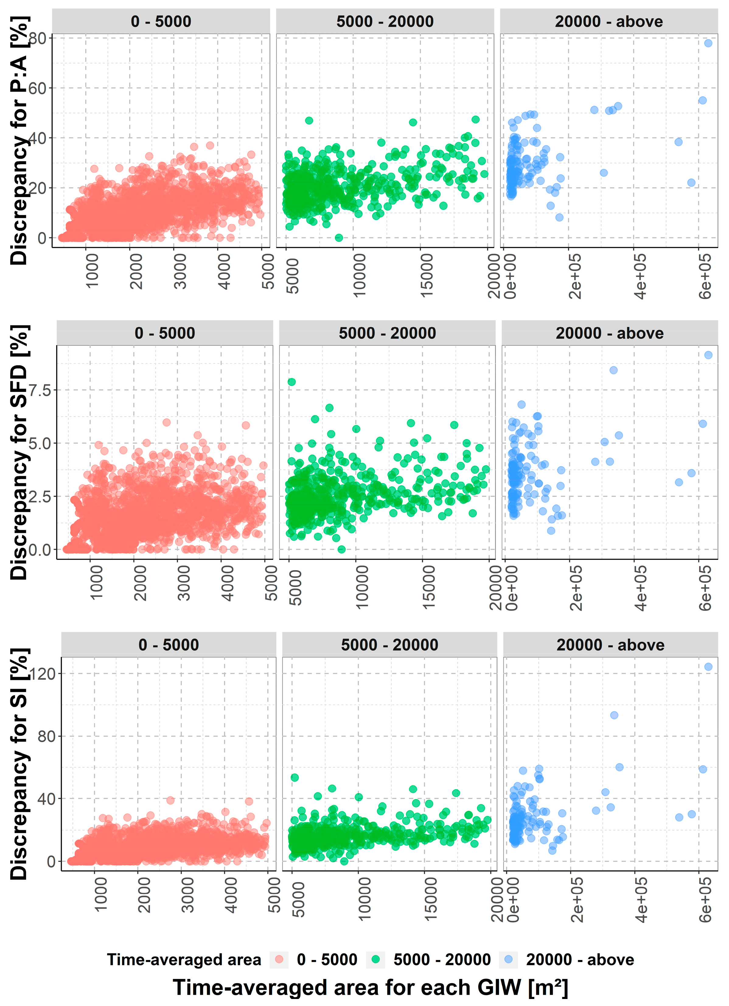
To assess the covariation of area and perimeter with time, as the wetness varies, similar to that obtained using the static data, the discrepancies between estimated shape metrics and the actual value at different times are evaluated (Figure 4). Discrepancies in SFD are found to be modest, ranging from 0 to 10%. In contrast, the discrepancies in the P:A ratio and SI estimates are found to be as large 80 and 120%, respectively. Notably, the discrepancies are usually higher for larger wetlands, irrespective of the metric.

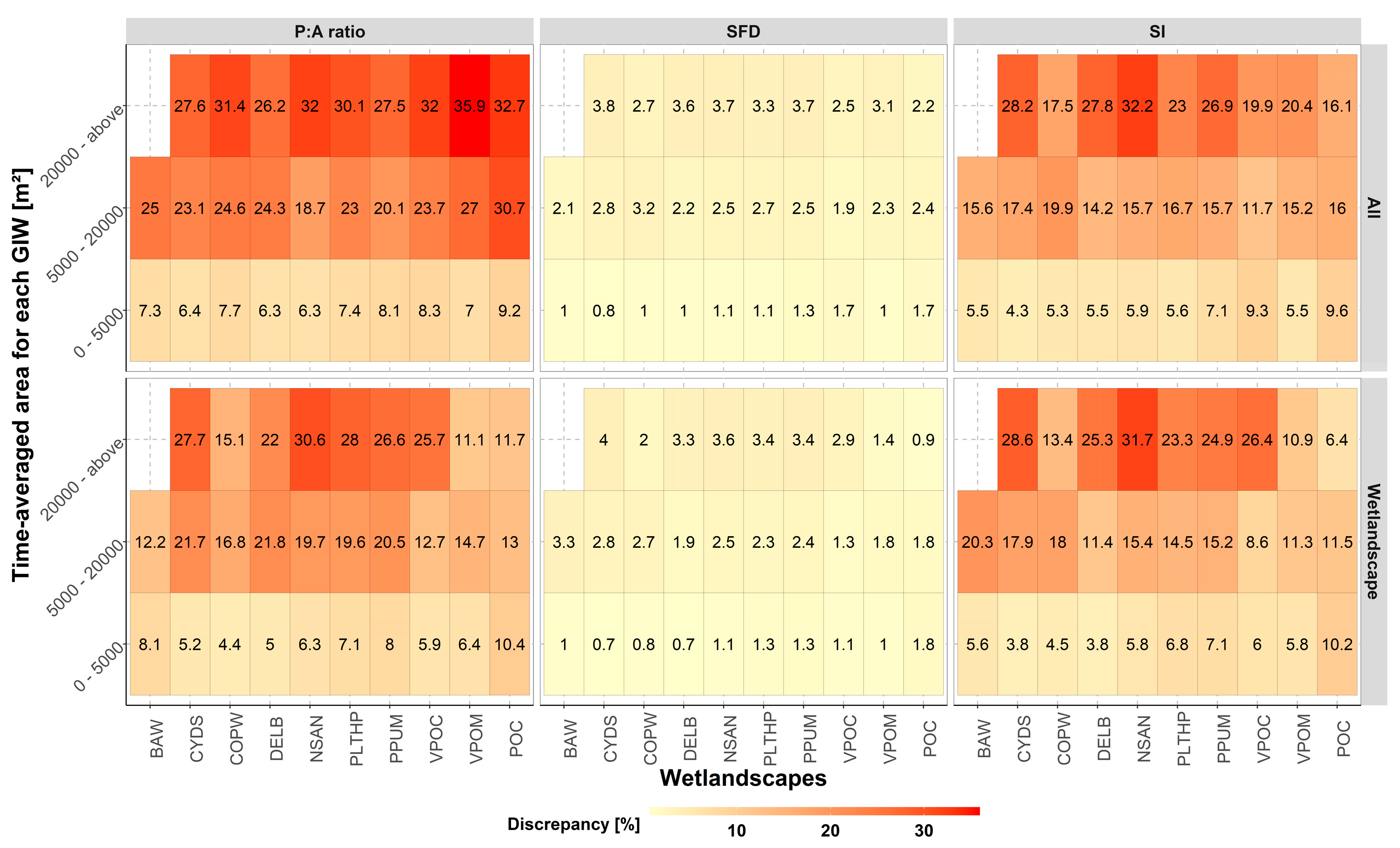
We further investigate if static relations that are developed specifically for individual wetlandscapes can be used to reduce discrepancies in the prediction of temporally evolving shape metrics. To this end, averaged prediction discrepancies are re-evaluated for each wetlandscape separately by using corresponding relations derived based on static data in those landscapes. Among the 87 cases (10 wetlandscapes * 3 wetland size groups − 3, see Figure 5), 69 cases (79.31%) show that the errors in estimated shape metrics reduce when static relations are developed using local data of the relevant wetlandscape. The corresponding fractions for the P:A ratio, SFD, and SI are 82.76%, 79.31%, and 75.86% (24/29, 23/29, and 22/29), respectively. Smaller errors in estimated shape metrics when developed using local data can be partially attributed to the similarity of the morphological and bathymetric characteristics of wetlands within a wetlandscape, even when they vary in size. In fact, if all wetlands in a wetlandscape exhibit an identical shape, the relationship between perimeter and area across different wetlands, as determined from static data, will resemble that derived from dynamic data. The largely uniform influence of hydrometeorological factors on inundation dynamics across wetlands within a wetlandscape is expected to also contribute to reduced errors in the estimation of shape metrics when obtained using static relations within a wetlandscape. On average, the impacts of reductions are the highest for large wetlands (Table S1). Among the ten wetlandscapes, discrepancy reduction is the highest (lowest) in Pocosins (Basin wetlands), with an average reduction of 36.28%, 26.07%, and 27.3.7% (20.12%, −28.57%, and −15.97%) for the P:A ratio, SFD, and SI, respectively.

4. Discussion

This study quantifies three well-known shape metrics for GIWs, viz. P:A ratio, SFD, and SI, and assesses their variations with wetland size. The results show that shape metrics have strong dependence on wetland size and inundation status. While this is unsurprising for shape metrics that are non-dimensionless, but even the SI metric, which is dimensionless, exhibits the influence of inundation status, i.e., what fraction of the wetland is inundated with respect to its maximal area, showing an increasing followed by a subsequently decreasing trend with inundation fraction. The results indicate that larger GIWs have more complex edges or non-rounded shapes compared to the smaller GIWs per unit area. The information regarding the variation of these shape metrics with wetland size can be used to design or restore wetlands with the goal to optimize the ecosystem service yield.

Next, the study evaluated the extent to which the shape metrics vs. wetland size relationship derived using static data, as has been achieved in the past, is valid for temporal datasets of wetland inundation extent. Evaluations for three well-known shape metrics, viz. P:A ratio, SFD, and SI, indicated that using relations derived from static data to estimate shape metrics at varying inundation extents introduced large discrepancies (up to 80%, 10%, and 120% for P:A ratio, SFD, and SI, respectively). Notably, these discrepancies are small for smaller wetlands. Overall, the results highlight the need to develop and incorporate temporally dynamic shape metrics or perimeter–area relationships to improve wetland function modeling. This is further corroborated by a recent study [77] that highlighted that the consideration of transient wetland inundation dynamics can increase nitrogen retention estimates by up to 130%. Given that the prediction errors reduced markedly when static relations were derived for each individual wetlandscape, the results underscore the need to develop perimeter–area relationships that are wetlandscape-specific. It is important to note that the shape factors considered here do not capture all aspects of wetland functions. Different wetland functions, such as recharge, nutrient cycling, habitat suitability, or carbon sequestration, may be more or less sensitive to wetland area and perimeter dynamics, and this relationship may change over time depending on changes in meteorological conditions and wetland substrate properties. Hence, the extent to which the temporally dynamic perimeter–area relationship may improve estimates of wetland functions are expected to be dependent on the ecosystem function under consideration, the representativeness of the shape metrics used to capture these functions, and site-specific properties. Despite this, the findings of this study clearly emphasize the necessity of relinquishing the limitations of static data analyses and embracing a more dynamic approach to shape metric assessment in models used for quantification of wetland ecosystem services.

References

- Whigham, D.F.; Chitterling, C.; Palmer, B. Impacts of Freshwater Wetlands on Water Quality: A Landscape Perspective. Environ. Manag. 1988, 12, 663–671. [Google Scholar] [CrossRef]
- Wamsley, T.V.; Cialone, M.A.; Smith, J.M.; Atkinson, J.H.; Rosati, J.D. The Potential of Wetlands in Reducing Storm Surge. Ocean Eng. 2010, 37, 59–68. [Google Scholar] [CrossRef]
- Ogawa, H.; Male, J.W. Simulating the Flood Mitigation Role of Wetlands. J. Water Resour. Plan. Manag. 1986, 112, 114–128. [Google Scholar] [CrossRef]
- Junk, W.J.; Brown, M.; Campbell, I.C.; Finlayson, M.; Gopal, B.; Ramberg, L.; Warner, B.G. The Comparative Biodiversity of Seven Globally Important Wetlands: A Synthesis. Aquat. Sci. 2006, 68, 400–414. [Google Scholar] [CrossRef]
- Pant, H.; Rechcigl, J.E.; Adjei, M. Carbon Sequestration in Wetlands: Concept and Estimation. Food Agric. Environ. 2003, 1, 308–313. [Google Scholar]
- Cheng, F.Y.; Van Meter, K.J.; Byrnes, D.K.; Basu, N.B. Maximizing US Nitrate Removal through Wetland Protection and Restoration. Nature 2020, 588, 625–630. [Google Scholar] [CrossRef]
- Cheng, F.Y.; Basu, N.B. Biogeochemical Hotspots: Role of Small Water Bodies in Landscape Nutrient Processing. Water Resour. Res. 2017, 53, 5038–5056. [Google Scholar] [CrossRef]
- Laterra, P.; Booman, G.C.; Picone, L.; Videla, C.; Orúe, M.E. Indicators of Nutrient Removal Efficiency for Riverine Wetlands in Agricultural Landscapes of Argentine Pampas. J. Environ. Manag. 2018, 222, 148–154. [Google Scholar] [CrossRef]
- Ligi, T.; Truu, M.; Truu, J.; Nõlvak, H.; Kaasik, A.; Mitsch, W.J.; Mander, Ü. Effects of Soil Chemical Characteristics and Water Regime on Denitrification Genes (NirS, NirK, and NosZ) Abundances in a Created Riverine Wetland Complex. Ecol. Eng. 2014, 72, 47–55. [Google Scholar] [CrossRef]
- Moreno-Mateos, D.; Mander, Ü.; Comín, F.A.; Pedrocchi, C.; Uuemaa, E. Relationships between Landscape Pattern, Wetland Characteristics, and Water Quality in Agricultural Catchments. J. Environ. Qual. 2008, 37, 2170–2180. [Google Scholar] [CrossRef]
- Bloom, A.A.; Bowman, K.W.; Lee, M.; Turner, A.J.; Schroeder, R.; Worden, J.R.; Weidner, R.; McDonald, K.C.; Jacob, D.J. A Global Wetland Methane Emissions and Uncertainty Dataset for Atmospheric Chemical Transport Models (WetCHARTs Version 1.0). Geosci. Model Dev. 2017, 10, 2141–2156. [Google Scholar] [CrossRef]
- Hondula, K.L.; DeVries, B.; Jones, C.N.; Palmer, M.A. Effects of Using High Resolution Satellite-Based Inundation Time Series to Estimate Methane Fluxes From Forested Wetlands. Geophys. Res. Lett. 2021, 48, e2021GL092556. [Google Scholar] [CrossRef]
- Melton, J.R.; Wania, R.; Hodson, E.L.; Poulter, B.; Ringeval, B.; Spahni, R.; Bohn, T.; Avis, C.A.; Beerling, D.J.; Chen, G.; et al. Present State of Global Wetland Extent and Wetland Methane Modelling: Conclusions from a Model Inter-Comparison Project (WETCHIMP). Biogeosciences 2013, 10, 753–788. [Google Scholar] [CrossRef]
- Zhang, Z.; Zimmermann, N.E.; Stenke, A.; Li, X.; Hodson, E.L.; Zhu, G.; Huang, C.; Poulter, B. Emerging Role of Wetland Methane Emissions in Driving 21st Century Climate Change. Proc. Natl. Acad. Sci. USA 2017, 114, 9647–9652. [Google Scholar] [CrossRef]
- Fairbairn, S.E.; Dinsmore, J.J. Local and Landscape-Level Influences on Wetland Bird Communities of the Prairie Pothole Region of Iowa, USA. Wetlands 2001, 21, 41–47. [Google Scholar] [CrossRef]
- Murray, C.G.; Kasel, S.; Loyn, R.H.; Hepworth, G.; Hamilton, A.J. Waterbird Use of Artificial Wetlands in an Australian Urban Landscape. Hydrobiologia 2013, 716, 131–146. [Google Scholar] [CrossRef]
- Santoro, A.; Chambers, J.M.; Robson, B.J.; Beatty, S.J. Land Use Surrounding Wetlands Influences Urban Populations of a Freshwater Turtle. Aquat. Conserv. Mar. Freshw. Ecosyst. 2020, 30, 1050–1060. [Google Scholar] [CrossRef]
- Wu, H.; Dai, J.; Sun, S.; Du, C.; Long, Y.; Chen, H.; Yu, G.; Ye, S.; Chen, J. Responses of Habitat Suitability for Migratory Birds to Increased Water Level during Middle of Dry Season in the Two Largest Freshwater Lake Wetlands of China. Ecol. Indic. 2021, 121, 107065. [Google Scholar] [CrossRef]
- Arp, C.D.; Jones, B.M.; Grosse, G. Recent Lake Ice-out Phenology within and among Lake Districts of Alaska, USA. Limnol. Oceanogr. 2013, 58, 2013–2028. [Google Scholar] [CrossRef]
- Bajer, P.G.; Beck, M.W.; Hundt, P.J. Effect of Non-Native versus Native Invaders on Macrophyte Richness: Are Carp and Bullheads Ecological Proxies? Hydrobiologia 2018, 817, 379–391. [Google Scholar] [CrossRef]
- Bélanger, L.; Couture, R. Use of Man-Made Ponds by Dabbling Duck Broods. J. Wildl. Manag. 1988, 52, 718–723. [Google Scholar] [CrossRef]
- Bowerman, W.W.; Grubb, T.G.; Bath, A.J.; Giesy, J.P.; Weseloh, D.V.C. A Survey of Potential Bald Eagle Nesting Habitat along the Great Lakes Shoreline; U.S. Department of Agriculture: Fort Collins, CO, USA, 2005; p. 6. [Google Scholar]
- Fox, B.J.; Holland, W.B.; Boyd, F.L.; Blackwell, B.F.; Armstrong, J.B. Use of Stormwater Impoundments near Airports by Birds Recognized as Hazardous to Aviation Safety. Landsc. Urban Plan. 2013, 119, 64–73. [Google Scholar] [CrossRef]
- Grubb, T.G.; Bowerman, W.W.; Bath, A.J.; Giesy, J.P.; Weseloh, D.V.C. Evaluating Great Lakes Bald Eagle Nesting Habitat with Bayesian Inference; RMRS-RP; U.S. Department of Agriculture: Fort Collins, CO, USA, 2003. [Google Scholar]
- Longcore, J.R.; Gibbs, J.P. Distribution and Numbers of American Black Ducks along the Maine Coast during the Severe Winter of 1980–1981. In Waterfowl in Winter; University of Minnesota Press: Minneapolis, MN, USA, 1988; pp. 377–389. [Google Scholar]
- Merendino, M.T.; Ankney, C.D.; Dennis, D.G. Increasing Mallards, Decreasing American Black Ducks: More Evidence for Cause and Effect. J. Wildl. Manag. 1993, 57, 199–208. [Google Scholar] [CrossRef]
- Merendino, M.T.; Ankney, C.D. Habitat Use by Mallards and American Black Ducks Breeding in Central Ontario. Condor 1994, 96, 411–421. [Google Scholar] [CrossRef]
- Oertli, B.; Parris, K.M. Review: Toward Management of Urban Ponds for Freshwater Biodiversity. Ecosphere 2019, 10, e02810. [Google Scholar] [CrossRef]
- Patton, D.R. A Diversity Index for Quantifying Habitat “Edge”. Wildl. Soc. Bull. 1975, 3, 171–173. [Google Scholar]
- Politi, E.; MacCallum, S.; Cutler, M.E.J.; Merchant, C.J.; Rowan, J.S.; Dawson, T.P. Selection of a Network of Large Lakes and Reservoirs Suitable for Global Environmental Change Analysis Using Earth Observation. Int. J. Remote Sens. 2016, 37, 3042–3060. [Google Scholar] [CrossRef]
- Roni, P.; Morley, S.A.; Garcia, P.; Detrick, C.; King, D.; Beamer, E. Coho Salmon Smolt Production from Constructed and Natural Floodplain Habitats. Trans. Am. Fish. Soc. 2006, 135, 1398–1408. [Google Scholar] [CrossRef]
- Willén, E. Phytoplankton and Water Quality Characterization: Experiences from the Swedish Large Lakes Mälaren, Hjälmaren, Vättern and Vänern. Ambio 2001, 30, 529–537. [Google Scholar] [CrossRef]
- Håkanson, L. The Length of Closed Geomorphic Lines. Math. Geol. 1978, 10, 141–167. [Google Scholar] [CrossRef]
- Håkanson, L. On Lake Bottom Dynamics—The Energy–Topography Factor. Can. J. Earth Sci. 1981, 18, 899–909. [Google Scholar] [CrossRef]
- Håkanson, L. Lake Bottom Dynamics and Morphometry: The Dynamic Ratio. Water Resour. Res. 1982, 18, 1444–1450. [Google Scholar] [CrossRef]
- Håkanson, L. Considerations on Representative Water Quality Data. Int. Rev. Der Gesamten Hydrobiol. Und Hydrogr. 1992, 77, 497–505. [Google Scholar] [CrossRef]
- Håkanson, L. Models to Predict Organic Content of Lake Sediments. Ecol. Model. 1995, 82, 233–245. [Google Scholar] [CrossRef]
- Håkanson, L. Error Propagations in Step-by-Step Predictions: Examples for Environmental Management Using Regression Models for Lake Ecosystems. Environ. Model. Softw. 1998, 14, 49–58. [Google Scholar] [CrossRef]
- Håkanson, L.; Kvarnäs, H.; Karlsson, B. Coastal Morphometry as Regulator of Water Exchange—A Swedish Example. Estuar. Coast. Shelf Sci. 1986, 23, 873–887. [Google Scholar] [CrossRef]
- Persson, J.; Håkanson, L.; Pilesjö, P. Prediction of Surface Water Turnover Time in Coastal Waters Using Digital Bathymetric Information. Environmetrics 1994, 5, 433–449. [Google Scholar] [CrossRef]
- Bernhardt, E.S.; Blaszczak, J.R.; Ficken, C.D.; Fork, M.L.; Kaiser, K.E.; Seybold, E.C. Control Points in Ecosystems: Moving Beyond the Hot Spot Hot Moment Concept. Ecosystems 2017, 20, 665–682. [Google Scholar] [CrossRef]
- Cohen, M.J.; Creed, I.F.; Alexander, L.; Basu, N.B.; Calhoun, A.J.K.; Craft, C.; D’Amico, E.; DeKeyser, E.; Fowler, L.; Golden, H.E.; et al. Do Geographically Isolated Wetlands Influence Landscape Functions? Proc. Natl. Acad. Sci. USA 2016, 113, 1978–1986. [Google Scholar] [CrossRef] [PubMed]
- Marton, J.M.; Creed, I.F.; Lewis, D.B.; Lane, C.R.; Basu, N.B.; Cohen, M.J.; Craft, C.B. Geographically Isolated Wetlands Are Important Biogeochemical Reactors on the Landscape. BioScience 2015, 65, 408–418. [Google Scholar] [CrossRef]
- McLaughlin, D.L.; Kaplan, D.A.; Cohen, M.J. A Significant Nexus: Geographically Isolated Wetlands Influence Landscape Hydrology. Water Resour. Res. 2014, 50, 7153–7166. [Google Scholar] [CrossRef]
- Van Meter, K.J.; Basu, N.B. Signatures of Human Impact: Size Distributions and Spatial Organization of Wetlands in the Prairie Pothole Landscape. Ecol. Appl. 2015, 25, 451–465. [Google Scholar] [CrossRef] [PubMed]
- Creed, I.F.; Lane, C.R.; Serran, J.N.; Alexander, L.C.; Basu, N.B.; Calhoun, A.J.K.; Christensen, J.R.; Cohen, M.J.; Craft, C.; D’Amico, E.; et al. Enhancing Protection for Vulnerable Waters. Nat. Geosci. 2017, 10, 809–815. [Google Scholar] [CrossRef] [PubMed]
- Walsh, R.; Ward, A.S. An Overview of the Evolving Jurisdictional Scope of the U.S. Clean Water Act for Hydrologists. WIREs Water 2022, 9, e1603. [Google Scholar] [CrossRef]
- Duan, H.; Xu, M.; Cai, Y.; Wang, X.; Zhou, J.; Zhang, Q. A Holistic Wetland Ecological Water Replenishment Scheme with Consideration of Seasonal Effect. Sustainability 2019, 11, 930. [Google Scholar] [CrossRef]
- Fu, Y.; Zhao, J.; Peng, W.; Zhu, G.; Quan, Z.; Li, C. Spatial Modelling of the Regulating Function of the Huangqihai Lake Wetland Ecosystem. J. Hydrol. 2018, 564, 283–293. [Google Scholar] [CrossRef]
- Hayashi, M.; van der Kamp, G. Simple Equations to Represent the Volume–Area–Depth Relations of Shallow Wetlands in Small Topographic Depressions. J. Hydrol. 2000, 237, 74–85. [Google Scholar] [CrossRef]
- Helzer, C.J.; Jelinski, D.E. The Relative Importance of Patch Area and Perimeter-Area Ratio to Grassland Breeding Birds. Ecol. Appl. 1999, 9, 1448–1458. [Google Scholar] [CrossRef]
- Yu, M.; Hu, G.; Feeley, K.J.; Wu, J.; Ding, P. Richness and Composition of Plants and Birds on Land-Bridge Islands: Effects of Island Attributes and Differential Responses of Species Groups. J. Biogeogr. 2012, 39, 1124–1133. [Google Scholar] [CrossRef]
- Krummel, J.R.; Gardner, R.H.; Sugihara, G.; O’Neill, R.V.; Coleman, P.R. Landscape Patterns in a Disturbed Environment. Oikos 1987, 48, 321–324. [Google Scholar] [CrossRef]
- Mandelbrot, B.B. Stochastic Models for the Earth’s Relief, the Shape and the Fractal Dimension of the Coastlines, and the Number-Area Rule for Islands. Proc. Natl. Acad. Sci. USA 1975, 72, 3825–3828. [Google Scholar] [CrossRef] [PubMed]
- Sugihara, G.; May, R.M. Applications of Fractals in Ecology. Trends Ecol. Evol. 1990, 5, 79–86. [Google Scholar] [CrossRef] [PubMed]
- Bertassello, L.E.; Rao, P.S.C.; Jawitz, J.W.; Botter, G.; Le, P.V.V.; Kumar, P.; Aubeneau, A.F. Wetlandscape Fractal Topography. Geophys. Res. Lett. 2018, 45, 6983–6991. [Google Scholar] [CrossRef]
- Gilbert, M.C.; Whited, P.M.; Clairain, J.; Smith, R.D. A Regional Guidebook for Applying the Hydrogeomorphic Approach to Assessing Wetland Functions of Prairie Potholes; U.S. Army Corps of Engineers: Washington, DC, USA, 2006. [Google Scholar]
- Wetzel, R.G. Limnology; W. B. Sauders Company: Philadelphia, 1975. [Google Scholar]
- Seekell, D.; Cael, B.B.; Byström, P. Problems with the Shoreline Development Index—A Widely Used Metric of Lake Shape. Geophys. Res. Lett. 2022, 49, e2022GL098499. [Google Scholar] [CrossRef]
- Jones, C.N.; Evenson, G.R.; McLaughlin, D.L.; Vanderhoof, M.K.; Lang, M.W.; McCarty, G.W.; Golden, H.E.; Lane, C.R.; Alexander, L.C. Estimating Restorable Wetland Water Storage at Landscape Scales. Hydrol. Process. 2018, 32, 305–313. [Google Scholar] [CrossRef] [PubMed]
- Lai, X.J.; Huang, Q.; Jiang, J.H. Wetland Inundation Modeling of Dongting Lake Using Two-Dimensional Hydrodynamic Model on Unstructured Grids. Procedia Environ. Sci. 2012, 13, 1091–1098. [Google Scholar] [CrossRef]
- Liu, Y.; Kumar, M. Role of Meteorological Controls on Interannual Variations in Wet-Period Characteristics of Wetlands. Water Resour. Res. 2016, 52, 5056–5074. [Google Scholar] [CrossRef]
- Sorribas, M.V.; Paiva, R.C.D.; Melack, J.M.; Bravo, J.M.; Jones, C.; Carvalho, L.; Beighley, E.; Forsberg, B.; Costa, M.H. Projections of Climate Change Effects on Discharge and Inundation in the Amazon Basin. Clim. Chang. 2016, 136, 555–570. [Google Scholar] [CrossRef]
- Wilson, M.; Bates, P.; Alsdorf, D.; Forsberg, B.; Horritt, M.; Melack, J.; Frappart, F.; Famiglietti, J. Modeling Large-Scale Inundation of Amazonian Seasonally Flooded Wetlands. Geophys. Res. Lett. 2007, 34, L15404. [Google Scholar] [CrossRef]
- Huang, C.; Peng, Y.; Lang, M.; Yeo, I.-Y.; McCarty, G. Wetland Inundation Mapping and Change Monitoring Using Landsat and Airborne LiDAR Data. Remote Sens. Environ. 2014, 141, 231–242. [Google Scholar] [CrossRef]
- Krapu, C.; Kumar, M.; Borsuk, M. Identifying Wetland Consolidation Using Remote Sensing in the North Dakota Prairie Pothole Region. Water Resour. Res. 2018, 54, 7478–7494. [Google Scholar] [CrossRef]
- Li, L.; Chen, Y.; Xu, T.; Liu, R.; Shi, K.; Huang, C. Super-Resolution Mapping of Wetland Inundation from Remote Sensing Imagery Based on Integration of Back-Propagation Neural Network and Genetic Algorithm. Remote Sens. Environ. 2015, 164, 142–154. [Google Scholar] [CrossRef]
- Shaeri Karimi, S.; Saintilan, N.; Wen, L.; Valavi, R. Application of Machine Learning to Model Wetland Inundation Patterns Across a Large Semiarid Floodplain. Water Resour. Res. 2019, 55, 8765–8778. [Google Scholar] [CrossRef]
- Pekel, J.-F.; Cottam, A.; Gorelick, N.; Belward, A.S. High-Resolution Mapping of Global Surface Water and Its Long-Term Changes. Nature 2016, 540, 418–422. [Google Scholar] [CrossRef]
- Jones, J.W. Efficient Wetland Surface Water Detection and Monitoring via Landsat: Comparison with in Situ Data from the Everglades Depth Estimation Network. Remote Sens. 2015, 7, 12503–12538. [Google Scholar] [CrossRef]
- Jones, J.W. Improved Automated Detection of Subpixel-Scale Inundation—Revised Dynamic Surface Water Extent (DSWE) Partial Surface Water Tests. Remote Sens. 2019, 11, 374. [Google Scholar] [CrossRef]
- Allen, G.H.; Pavelsky, T.M. Global Extent of Rivers and Streams. Science 2018, 361, 585–588. [Google Scholar] [CrossRef] [PubMed]
- Luijendijk, A.; Hagenaars, G.; Ranasinghe, R.; Baart, F.; Donchyts, G.; Aarninkhof, S. The State of the World’s Beaches. Sci Rep 2018, 8, 6641. [Google Scholar] [CrossRef]
- Mentaschi, L.; Vousdoukas, M.I.; Pekel, J.-F.; Voukouvalas, E.; Feyen, L. Global Long-Term Observations of Coastal Erosion and Accretion. Sci Rep 2018, 8, 12876. [Google Scholar] [CrossRef]
- Park, J.; Kumar, M.; Lane, C.R.; Basu, N.B. Seasonality of Inundation in Geographically Isolated Wetlands across the United States. Environ. Res. Lett. 2022, 17, 054005. [Google Scholar] [CrossRef]
- Lane, C.R.; D’Amico, E. Identification of Putative Geographically Isolated Wetlands of the Conterminous United States. J. Am. Water Resour. Assoc. 2016, 52, 705–722. [Google Scholar] [CrossRef]
- Cheng, F.Y.; Park, J.; Kumar, M.; Basu, N.B. Disconnectivity Matters: The Outsized Role of Small Ephemeral Wetlands in Landscape-Scale Nutrient Retentions. Environ. Res. Lett. 2022, 18, 024018. [Google Scholar] [CrossRef]
Figure 1.
Ten 1000 km2 rectangular wetlandscapes and identified NWI GIWs in them, as derived in [75]. The ten wetlandscapes include the Basin wetlands (BAW), Cypress domes of the Southeast (CYDS), Coastal plain wetlands (COPW), Delmarva bays (DELB), Nebraska Sandhills (NSAN), Playa lakes of Texas and High Plains (PLTHP), Prairie potholes of the Upper Midwest (PPUM), Vernal pools of California (VPOC), Vernal pools of Maine (VPOM), and the Pocosins (POC).
Figure 2.
P:A ratio, shoreline fractal dimension (SFD), and shoreline irregularity (SI) vs. time-averaged area for GIWs belonging to different size-groups. The three groups contain GIWs with time-averaged size falling within the range of 0–5000 m2, 5000–20,000 m2, and 20,000 m2 and above. Each point indicates the metric magnitude for a given GIW. The black line represents the best non-linear LOESS fit.
Figure 3.
P:A ratio, shoreline fractal dimension (SFD), and shoreline irregularity (SI) vs. wetness fraction of GIWs belonging to different size-groups. The three groups contain GIWs with their time-averaged size falling within the range of 0–5000 m2, 5000–20,000 m2, and 20,000 m2 and above. Twenty equal-sized bins are used in the x-axis of each panel.
Figure 4.
Prediction discrepancies of P:A ratio, shoreline fractal dimension (SFD), and shoreline Irregularity (SI) vs. area of each GIW belonging to different size-groups. The three groups contain GIWs with their time-averaged size falling within the range of 0–5000 m2, 5000–20,000 m2, and 20,000 m2 and above. Each point indicates the time-averaged discrepancies for a GIW when the dynamic metrics were predicted by the empirical relation obtained from static wetland descriptors such as its maximum area and perimeter.
Figure 5.
Heatmap with prediction discrepancies of P:A ratio, shoreline fractal dimension (SFD), and shoreline irregularity (SI) vs. area of GIWs belonging to different size-groups in each wetlandscape. The prediction used the static shape relations vis à vis wetland size from all wetlandscapes (top row) or the given wetlandscape (bottom row). The three size-groups contain GIWs with time-averaged size in the range of 0–5000 m2, 5000–20,000 m2, and 20,000 m2 and above.
Disclaimer/Publisher’s Note: The statements, opinions and data contained in all publications are solely those of the individual author(s) and contributor(s) and not of MDPI and/or the editor(s). MDPI and/or the editor(s) disclaim responsibility for any injury to people or property resulting from any ideas, methods, instructions or products referred to in the content. |
© 2023 by the authors. Licensee MDPI, Basel, Switzerland. This article is an open access article distributed under the terms and conditions of the Creative Commons Attribution (CC BY) license (https://creativecommons.org/licenses/by/4.0/).
Share and Cite
MDPI and ACS Style
Park, J.; Kumar, M.; Jones, C.N. Modeling Wetland Functions: Is Space-to-Time Substitution of the Perimeter–Area Relationship Appropriate? Water 2023, 15, 3445. https://doi.org/10.3390/w15193445
AMA Style
Park J, Kumar M, Jones CN. Modeling Wetland Functions: Is Space-to-Time Substitution of the Perimeter–Area Relationship Appropriate? Water. 2023; 15(19):3445. https://doi.org/10.3390/w15193445
Chicago/Turabian StylePark, Junehyeong, Mukesh Kumar, and C. Nathan Jones. 2023. "Modeling Wetland Functions: Is Space-to-Time Substitution of the Perimeter–Area Relationship Appropriate?" Water 15, no. 19: 3445. https://doi.org/10.3390/w15193445
Note that from the first issue of 2016, this journal uses article numbers instead of page numbers. See further details here.