Article

Planning and Evaluating Nature-Based Solutions for Watershed Investment Programs with a SMART Perspective Using a Distributed Modeling Tool

1
Gotta Ingeniería S.A.S., Medellín 050030, Colombia
2
The Nature Conservancy, Bogotá 110231, Colombia
3
The Nature Conservancy, Wellington 6012, New Zealand
*
Author to whom correspondence should be addressed.
Water 2023, 15(19), 3388; https://doi.org/10.3390/w15193388
Submission received: 18 August 2023 / Revised: 14 September 2023 / Accepted: 21 September 2023 / Published: 27 September 2023
(This article belongs to the Special Issue Integrated Water Resources Modeling and Management)

Abstract

:
Watershed Investment Programs (WIPs) face many challenges in implementing strategies aimed at restoring and preserving ecosystem services using Nature-based Solutions (NbS). A key challenge lies in defining SMART (Specific, Measurable, Achievable, Relevant, and Time-bound) objectives, which involve addressing questions such as which NbS interventions to apply, where, and in what amounts. Effectively achieving WIPs’ objectives requires strategic implementation of NbS. In response to this challenge, we present SIGA-CALv1.0, a daily time-step and distributed modeling conceptual framework that enables the design and evaluation of the impact of NbS portfolios on water quantity and quality. To validate our framework, we applied it to the Arma river basin in Colombia. Our findings indicate that NbS can lead to substantial benefits, including reductions of up to 47% in sediment, 62% in nitrogen, 8% in phosphorus, and 15% in pathogen indicators (total coliforms). The proposed methodological framework offers decision-makers robust technical support for defining strategic NbS implementation plans, guided by SMART objectives. This approach strengthens the effectiveness of ecosystem services restoration and conservation strategies in watersheds, enabling more efficient resource allocation and improved environmental outcomes.

1. Introduction

Nature-based solutions (NbS) are increasingly being implemented as strategies to address water security issues [1,2,3], with growing use and replicability in watershed investment programs (WIPs) in urban and rural areas worldwide. One of the primary challenges in implementing NbS strategies is aligning them with SMART (Specific, Measurable, Achievable, Relevant, and Time-bound) objectives, particularly when funding is limited, and key stakeholders prioritize measurable and near-term outcomes.
The effectiveness of NbS investments in improving water quantity and quality is commonly defined, either based on a conceptual formulation of the likely changes in the physical processes directly or indirectly modified through the portfolio of NbS investments, or by comparing measured data regarding water quantity and quality from impact, reference, and control watersheds [4,5,6]. However, expected outcomes are often complex and are sensitive to local conditions, such as climate, aridity, geology, and watershed size [7,8], as well as external and anthropogenic disturbances. This makes practically evaluating NbS investment programs challenging [9]. Monitoring and modeling therefore arise as complementary quantitative strategies to support NbS investments, especially because the effects of many NbS take time to manifest.
Modeling tools, such as the Soil Water Assessment Tool (SWAT) [10] and the Integrated Valuation of Ecosystem Services and Tradeoffs Tool (InVEST) [11], are widely recognized for their ability to quantify several water quantity and quality attributes at different temporal and spatial scales (see Table 1). The InVEST tool is typically more user-friendly for those not as familiar with process-based modeling [7] and enables long-term assessments for a variety of water quantity and quality metrics, but its temporal structure limits the assessment of stream flow regimes that are required to connect the effects of NbS with changes in extreme hydrological events such as floods and droughts. This limitation can make it challenging to obtain relevant indicators from InVEST to guide decision making in certain contexts. Conversely, a comprehensive review of global applications of the SWAT tool for assessing ecosystem service responses to NbS was conducted by [12], with most documented cases focusing on provisioning and regulating services, including those presented in Table 1. The set of parameters required to represent NbS in the SWAT tool is also well documented [13,14] for agricultural best management practices, such as contour farming and no-tillage farming. Furthermore, the semidistributed structure of the SWAT tool has been used to identify priority management areas (PMAs) within watersheds [15] based on the pollutants exported to surface waterways from the nearby subbasins and hydrological response units (HRUs) that are used to spatially discretize watersheds. However, it is important to note that in practice, intervention areas do not necessarily fit the size or extent of HRUs because many WIPs (e.g., Water Funds) [16] typically focus on spatial units corresponding to parcels of land (hereafter ‘parcels’) owned or controlled by single persons or entities. The aforementioned challenges have been of interest to stakeholders, research centers, universities, and consulting companies in relation to both research and operational tasks [17], leading to the development of several comprehensive tools for hydrological analyses and modeling based on conceptual models [17,18,19,20]. In this paper, we present an alternative model for WIPs, which we have called SIGA-CALv1.0, which overcomes some modeling challenges related to the spatial representation of hydrological, sedimentological, and water quality processes. Table 1 shows some general attributes for SIGA-CALv1.0 in comparison with SWAT and InVEST, which are also widely used in NbS investment analysis for watersheds.
We aim to describe a comprehensive framework for quantifying the water quantity and quality effects of existing and potential NbS interventions and prioritizing the spatial allocation of NbS within a watershed based on these effects. This framework is based on the conceptually based, daily time-step, distributed and cell-based modeling tool SIGA-CALv1.0 (from the Spanish acronym for Geoscientific Open Simulation), developed and implemented by The Nature Conservancy and Gotta Ingeniería to support the Water Fund CuencaVerde (based in Medellín, Colombia) to define and develop SMART-oriented NbS interventions as laid out in Table 2 below.

2. Materials and Methods

We have used a distributed modeling approach to prioritize NbS interventions in certain areas of a watershed, based on the assessment of several important environmental variables under different scenarios. This section outlines the modeling framework structure and its key concepts, as well as the case study used to perform the analysis.

2.1. Modeling Framework Structure

SIGA-CAL is a computational modeling framework based on the modeling scheme SHIA proposed by [18], which has been developed to represent different basin phenomena. The resulting framework integrates six models that operate on a daily time step basis and represent different aspects of watersheds (meteorology, phenology, hydrology, sedimentology, landslides, and water quality) in a distributed manner. The watershed is spatially delimited into square grid cells to enable the modeling process.
At each time step, the modeling framework performs different calculations in sequence. First, it calculates the meteorological variables of interest for all the cells in the watershed. After that, the leaf area index (LAI) is computed through a phenological model, giving information about the state of the vegetation in each cell. The hydrological model is executed next, incorporating the information provided by the former two models (meteorology and phenology). The runoff information given by the hydrological model enables the computing of the landslides and sedimentological models. The water quality model is a composite of several submodels, one each for temperature, dissolved oxygen, ammonium, organic nitrogen, nitrates, organic phosphorus, inorganic phosphorus, Escherichia coli, biochemical oxygen demand, and conductivity.
Given that the base model (SHIA) is a hydrological tank model, the sedimentology and water quality models (in hillslopes) have been conceptualized in a similar way. Section 2.2 provides a more detailed explanation of the conceptual framework and mathematical models used in SIGA-CALv1.0.

2.2. Topological Representation of the Basin

SIGA-CALv1.0 models the basin as a raster grid made up of square cells. Several distributed attributes give information about flow conditions, terrain morphology, and the state of each cell regarding all the models of the framework (e.g., LAI, water depth storage in the aquifer, and organic nitrogen concentration).
Among the attributes of each cell is a type (channel network or hillslope), which determines which processes may occur in the cell for the several models previously described. Connection between cells is defined by the destination attribute, which specifies the identification number of the cell to which the given cell’s drainage is directed, based on the flow direction [21]. Given a set of initial conditions, as well as the distributed parameters of the basin, the modeling framework continuously updates the state of all the cells for all the variables at each time step until the simulation is finished.

2.3. Physical Processess Conceptualization

As indicated previously, SIGA-CALv1.0 is a composite modeling framework made up of several integrated models that have been independently proposed by different authors, adapted to the framework structure. Measuring units have been standardized: mass is always expressed in kilograms, length in meters, and time in days. The sections below outline each model in turn. The details of each model, including their mathematical formulation and empirical relationships, can be found in the Supplementary Material S1.

2.3.1. Meteorological Model

This model represents the spatial and temporal variability of the meteorological variables needed to simulate the phenological and hydrological processes of the watershed, based on the interpolation of point measured time-series data. Relative humidity, solar radiation, vertical precipitation (rainfall), and zonal and meridional wind speed are interpolated using the inverse distance weighting (IDW) method [22]. Minimum and maximum temperatures are interpolated using an assembly of the IDW method with the ordinary least squares (OLS) method [23]. The OLS method is used to incorporate the trend component of air temperature as a variable dependent on altitude, while the IDW method is used to interpolate the residual spatial variability.
Potential evapotranspiration is evaluated using one of two approaches depending on the cell conditions: in channel network type cells, evapotranspiration is calculated using the method proposed by Shuttleworth [24], whereas the FAO Penman–Monteith model is used in hillslope type cells [25]. Actual evapotranspiration is evaluated within the hydrological model.
Horizontal precipitation (fog interception by vegetation) is evaluated after the phenological model—because it depends on the state of the vegetation—using the approach proposed by [26]. With this approach, horizontal precipitation is calculated based on temperature, relative humidity, LAI, wind velocity, and a land-cover-specific fog collection efficiency. Horizontal precipitation is given in the same units as vertical precipitation depth (meters), and total precipitation for each cell is calculated as a sum of vertical and horizontal precipitation.

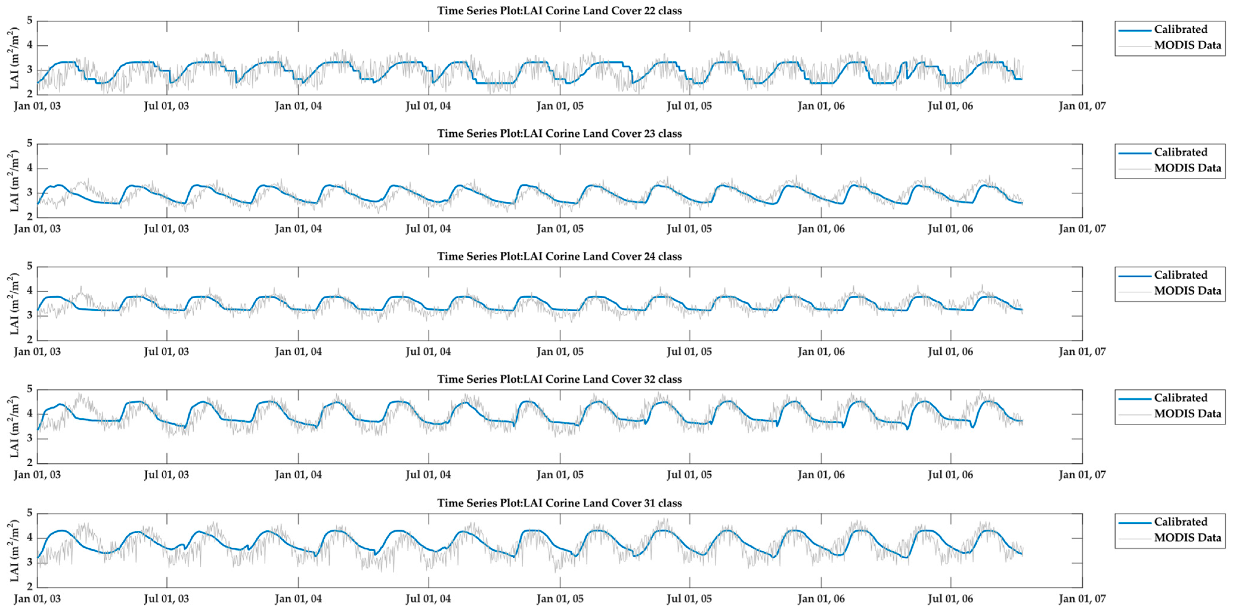
2.3.2. Phenological Model

Changes in vegetation driven by environmental conditions can be represented by SIGA-CALv1.0 through its phenological model, based on [27]. Assuming a permanent state of vegetation (maturity), two phases can be identified: growth (increase in leaf surface) and senescence (decrease in leaf surface). The growth and senescence phases can be expressed in terms of leaf area index (LAI), which is defined as the one-sided green leaf surface per unit ground surface area (m2/m2) [28].
LAI increase is determined using air temperature, until a land-cover-specific maximum LAI value is reached, at which point the growth phase stops and LAI remains constant until the senescence rate (leaf aging and death) overtakes the growth rate. During senescence, LAI declines until a land-cover-specific minimum LAI value is reached, and/or environmental conditions (soil moisture and precipitation regime) enable a new growth phase to start.
Some important variables for subsequent models depend on LAI, including the value of the Manning’s roughness coefficient in hillslopes, and the cropping management factor of the Universal Soil Loss Equation (RUSLE C factor). Manning’s coefficient in hillslopes has two components: one based on soil texture and other based on vegetation conditions. The vegetation component is calculated by multiplying a land-cover-specific potential Manning’s coefficient with a fraction given by the quotient of the current LAI value and the maximum potential LAI value for the corresponding land cover of the cell.
The RUSLE C factor is one of the variables for the estimation of sediment transport capacity in hillslopes using the modified version of the Kilinic and Richardson equation [29], as adapted by Julien [30]. It is evaluated as a function of LAI using an empirical relationship (see Supplementary Material S2).

2.3.3. Hydrological Model

The SHIA model [18] is the basis of the hydrology of the SIGA-CAL modeling framework. SHIA is a distributed hydrological model that represents the surface and soil layers of a watershed as storage tanks, connected by pipes both vertically (inside a single cell) and horizontally (between an origin cell and a destination cell). It assumes that water flow is vertical through the surface and soil layers until certain thresholds are reached, at which point excess water is temporarily stored and then drained horizontally to the destination cell, flowing through the same layer where the water excess has occurred. The channel network cells are an exception to this last rule, as the horizontal drainage goes directly to the channel storage tank of the same cell.
To incorporate the concept of preferential flow pathways, the vertical connection within each cell is represented by a main pipe with consecutive diversion nodes that deliver the water to the different storage tanks.
Water enters the system from the top of the pipe as total precipitation, flowing down until it finds the first diversion node where some water is sent to the foliar storage (tank 0), representing the process of water retention by vegetation via surface tension. The amount of water conducted to foliar storage depends on the amount of total precipitation, as well as the remaining capacity of the tank, which is finite. The total capacity of the foliar storage depends on the leaf surface in the cell, which is given by the LAI. Water stored in the foliar tank cannot join runoff flow, and its only way out is via evaporation.
Any water remaining in the main pipe after the first diversion node continues its way down to the next diversion node, which transfers water to the capillary storage (tank 1). This diversion represents the process of water retention and storage in the soil micropores, where it cannot flow by the effect of gravity. The amount of water transferred to the capillary storage depends on the amount of water available at the input of the corresponding diversion node (not-intercepted precipitation) as well as the remaining capacity of the capillary storage tank. The total capacity of the capillary storage is the volume of water that must be added to bring the soil column of a cell from the permanent wilting point to field capacity. Similarly, to the water stored in the foliar tank, water stored in the capillary tank cannot join runoff flow; its only way out is via transpiration by the vegetation.
Any water still available after the capillary diversion node keeps going down until it reaches the superficial storage (tank 2) diversion node. The superficial storage tank represents the water that flows over the hillslope surface. The amount of water that enters the superficial storage tank depends on the water available at the input of the corresponding diversion node (effective precipitation) as well as the upper soil permeability (which describes the capacity of the soil to receive infiltration from the surface). When the upper soil layer becomes saturated, water can emerge to the surface and become another input for the superficial storage tank. Since water infiltrating to the upper soil has already been subtracted at the diversion node, the only way out of the superficial storage is the horizontal drainage to the destination cell, or in the case of channel network cells to the channel storage tank of the same cell.
Any remaining water in the main pipe after the superficial diversion node flows downward to the upper soil storage (tank 3) diversion node. This point represents the process of infiltration and percolation through the macropores, which are the spaces within the shallow layer of soil where water is subject to the force of gravity. The quantity of water entering the upper soil storage depends on the water available at the input of the corresponding diversion node (infiltration) and the lower soil permeability (which determines the capacity of the deeper soil layer to receive percolation from the upper layer). Since water percolating to the lower soil has been already accounted for at the diversion node, the water stored within the upper soil tank can either be drained horizontally to the destination cell (or to the channel storage tank of the same cell in the case of channel network cells), or it can emerge directly to the superficial tank if the capacity of the upper soil storage has been exhausted (i.e., it is fully saturated). The upper soil storage capacity is the amount of water that must be added to bring the soil column of a cell from field capacity to saturation; water emergence occurs when saturation conditions are reached.
Finally, water remaining in the main pipe (if any) reaches the final diversion node. At this point it is possible to incorporate underground water exchange between watersheds, resulting in an addition or a subtraction of the quantity of water that is finally delivered to the lower soil storage (tank 4). However, underground water exchanges between watersheds should be incorporated only when there is strong evidence supporting their occurrence, and therefore, they are generally not considered. Water transferred to the lower soil storage flows at a very low velocity and can only leave the tank via horizontal drainage to the destination cell (or to the channel storage tank of the same cell in the case of channel network cells).
Channel storage (tank 5) is only present in the cells where permanent and consolidated drainage channels exist. This tank receives water drained horizontally from the channel storage of the upstream channel network cell(s), as well as the horizontal drainage coming from the superficial, upper soil, and lower soil storage tanks of the same cell. The only way out of the channel storage tank is the horizontal drainage to the channel storage of the destination cell.
Anthropic interventions in the hydrologic system, such as reservoirs, water intakes, and discharges, are included in the model. Reservoir cells are represented as simple channel storage tanks, in which only surface processes are considered: there is an exchange of water between the water body and the atmosphere through precipitation and evaporation, and horizontal transport of liquid water from the origin to the destination cell channel storage tanks. Water intakes and discharges are modeled as additions or removals of water from the channel storage tanks of their respective cells.
Figure 1a schematically presents the conceptualization of the hydrological model (other parts of the Figure visualize the other models, which are explained below).

2.3.4. Sedimentological Model

Sediment production, transport, and deposition processes are simulated in the SIGA-CAL modeling framework by incorporating the CASC2D-SED sediment model [31] along with the fundamental principles of the hydrological tank model. A riverbank erosion component is also integrated, using the work of Wilkinson [32]. The sediment dynamics are governed by the availability of sediment (supply) and the energy availability of the water flow to move particles (transport capacity). Erosion prevails when the transport capacity exceeds the sediment supply, whereas deposition dominates when sediment supply surpasses transport capacity. A balance between capacity and supply promotes transport only (no erosion or deposition).
The previously outlined concepts are represented in SIGA-CALv1.0 through a system of storage tanks and flow paths, with sediments being the flowing element. Each cell in the model is equipped with a minimum of three storage tanks: one for suspended material at the top, another for deposited material in the middle, and a third for parental material at the bottom; all of them together representing the hillslope component of sediment dynamics. Channel network cells feature three additional storage tanks that are analogous to the ones described earlier, but specific to the river channel itself. The main distinction of the channel-specific storage tanks is that the parent material within them consists of riverbank material, whereas in the hillslope storage tanks it is composed of the upper reach of the soil. Each one of the tanks is further divided into three subtanks, assigned to the three particle sizes considered by the model (sand, silt, and clay).
As mentioned above, the volume of sediment flow is determined by the transport capacity of water. For hillslopes, the modified version of the Kilinic and Richardson equation [29], as adapted by Julien [30], is used to evaluate this variable. In the case of channel networks, transport capacity is determined using the Engelund and Hansen equation [33]. The magnitude of the transport capacity in each cell dictates the volume of sediment that can flow horizontally as suspended material.
The first process that occurs in each time step is deposition from the suspended material to the deposited material tank of each cell. The sediment settling process follows the same methods explained by [17,34], which are also based in the CASC2D-SED model. The volume of sediment settled is subtracted from the suspended material tank and added to the deposited material tank.
Following sediment deposition, the model compares the transport capacity with the volume of material stored in the suspended material tank. If the volume of material exceeds the transport capacity, an amount equal to the transport capacity is moved horizontally, and the remaining volume in the suspended material tank is then subjected to the deposition process in the next time step. Conversely, if the transport capacity exceeds the volume of material in the suspended material tank, all its contents are horizontally mobilized as suspended material, and the remaining transport capacity is utilized to mobilize sediments stored in the deposited material tank.
A similar process is performed for the deposited material tank. If the volume of material stored in the deposited material tank exceeds the remaining transport capacity, a volume equivalent to the remaining transport capacity is removed from the deposited material tank and mobilized horizontally, as resuspended material. Alternatively, if the remaining transport capacity is greater than the volume of material stored in the deposited material tank, all of it is resuspended. If this occurs, the remaining transport capacity after mobilizing suspended material and resuspending sediment is used to remove and mobilize material from the parental material tank in the case of hillslopes, representing the erosion process over the surface of the soil. As mentioned earlier, erosion in the channel network is modeled using the Wilkinson approach.
The horizontal mobilization of suspended, resuspended, and eroded material is similar to the horizontal drainage of the tanks in the hydrological model. In hillslope cells, all the mobilized material is sent to the suspended material tank of the corresponding destination cell. Since channel network cells feature both hillslope and channel-specific tanks, their hillslope mobilized material is sent to the channel suspended material tank of the same cell, whereas their channel mobilized material is sent to the channel suspended material tank of the corresponding destination cell. Figure 1b schematically presents the conceptualization of the sedimentological model.

2.3.5. Landslide Model

Mass movements are simulated in SIGA-CALv1.0 using a mechanistic geotechnical approach relying on the SHIA Landslide model [35], which builds upon earlier research by [36]. The susceptibility of a specific cell to experience a landslide is evaluated through the infinite slope model [37]. This model considers the various stabilizing and destabilizing forces acting on a simplified conceptual slope.
These forces are affected by several variables, namely soil bulk density, soil cohesion, soil friction angle, water density, soil vertical depth, vertical depth of the saturated portion of the soil, and slope angle. Among these variables, only the vertical depth of the saturated portion of the soil is modelled for each time step in SIGA-CALv1.0. This variation is coupled with the hydrological model, since it is evaluated using the amount of water stored in the upper soil tank, as well as the soil depth and the maximum capacity of the upper soil storage.
Since the vertical depth of the saturated portion of the soil is the only time-changing variable in SIGA-CALv1.0, a critical landslide-triggering value for the variable can be calculated for each cell based on the mechanical equilibrium of the forces involved in the infinite slope system. That critical value is the main tool used to perform the slope stability analysis.
That being said, some cells can be excluded from the stability analysis for two reasons. Cells where the soil vertical depth is smaller than the critical value of the saturated soil depth have a correspondingly unconditionally stable hillslope, and therefore no landslides ever occur in these cells. Cells in which destabilizing forces dominate even when there is no water stored in the upper soil tank (saturated soil depth is zero) are considered unconditionally unstable. For these unconditionally unstable cells, it is assumed that a landslide already occurred before the start of the simulation.
During the simulation, the slope stability analysis is performed at every time step for each one of the susceptible cells (all those that have not been previously excluded). The vertical depth of the saturated portion of the soil is compared to the corresponding critical value, and a landslide is triggered at those cells where the critical value is surpassed. Landslides are represented as a mass movement process, started by removing a volume of sediment from the cell. The removed volume is calculated using an expression based in [38] (refer to the Supplementary Material S1).
The landslide development is modeled using the method proposed by [36]. The movement is sent to the corresponding destination cell, where it keeps removing material successively until a cell with a slope angle less than a specified critical value (usually between 10° and 15°) is reached. Sediment deposition starts at the next cell, and continues until either a runout distance is depleted or a cell with a slope angle less than a specified stop value (usually between 4° and 5°) is reached (whichever condition is satisfied first).
The runout distance is estimated as a fraction (usually set to 0.45) of the difference between the elevation of the cell where the landslide is triggered and the elevation of the cell where the material removal stops. The volume of material accumulated along the removal path is divided across the runout distance, and it is distributed along the deposition cells according to their distance along the direction of drainage.
If the movement stops due to reaching a slope angle less than the stop value (without depleting the runout distance), all the remaining material is deposited in the stop cell.
All deposited material is directed to the deposited storage tank of the sedimentological model in the corresponding cells. Figure 1c presents a conceptual schematic of the landslide model.

2.3.6. Water Quality Model

SIGA-CALv1.0 features a water quality model that accounts for the impact of both nonpoint source and point source loads on the physical and chemical properties of water as it flows through the channel network. This works by representing water quality processes using two distinct approaches: one for hillslopes and another for river channels.
On hillslopes, diffuse loads of organic nitrogen, nitrates, ammonium, organic phosphorus, inorganic phosphorus, and E. coli, all dependent on land cover, are applied over the soil surface of each cell. Their dilution, transport, and transformation processes are represented through a system of storage tanks and flow paths that follow the structure of the hydrological model. The representation of these processes in SIGA-CALv1.0 is based on the conceptualization of the SWAT, TETIS, and INCA models [39,40,41,42], as shown in Figure 1d.
A daily mass of the determinant enters the accumulation storage tank, located at the top of the system. The mass stored in this tank can undergo processes such as washing, transformation by bacterial action, volatilization, and absorption by plants. Water dilution occurs when a precipitation event takes place, as effective precipitation washes a portion of the mass proportional to a determinant-specific solubility constant. The washed portion is then directed to the capillary storage diversion node.
At this point, the mass of the determinant dissolved in the water entering the capillary hydrological storage is delivered to the homologous water quality tank. The mass dissolved in the water that continues flowing down through the main pipe of the hydrological model reaches the superficial storage diversion node.
In general, since the mass of the determinant is dissolved in the water, the distribution of water quality determinants closely follows the distribution of water in the hydrological model, except for the diffusion-based mixing between the mass of dissolved determinant in the upper soil storage tank and the capillary storage tank. The capillary storage tank consists of two sections, a saturated and a partially saturated portion. The partitioning between these sections affects only the water quality model, as only the saturated portion of the capillary tank can mix with the content of the upper soil tank.
The horizontal drainage also follows the behavior of the hydrological model, within the superficial, upper soil, and lower soil tanks. Water quality determinants are drained horizontally through the hillslope cells until they reach a channel network cell. Just like in the hydrological model, channel network cells have both the hillslope tank structure and a channel-specific structure. Again, in channel network cells, the horizontal drainage from the hillslope tank structure is directed to the channel structure, where the water quality determinants follow a different mechanism of transport.
During their path along the hillslopes, water quality determinants undergo different transformation, gain, and/or loss processes. These processes only occur in the reactive zone, where temperature and humidity conditions lead to transformations taking place. The reactive zone is composed of all the storage tanks and derivations located above the lower soil diversion node.
The transformation processes occurring in the reactive zone are specific for each water quality determinant. The different forms of nitrogen can follow the processes of mineralization, nitrification, denitrification, fixation, volatilization, immobilization, and plant uptake. Organic and inorganic phosphorus can undergo the processes of mineralization, immobilization, plant uptake, and exchange with the firmly soil-bound phosphorus pool. Finally, E. coli related processes include growth and die-off.
In the nonreactive zone, the water quality determinants are only transported without other processes taking place, with the exception of E. coli, for which all the content entering the nonreactive zone is considered lost. This is because it is assumed that E. coli cannot survive under the environmental conditions present in the lower soil storage tank.
In river channel cells, water quality determinant loads are received from both hillslopes and water discharges. These loads result from the processes of dilution, transport, and transformation of diffuse loads in the upstream hillslopes, as well as from point sources (water discharges) into the network. Additional variables are modeled in the channel network besides those considered in the hillslope cells, namely: total phosphorus, dissolved oxygen, biochemical oxygen demand, temperature, conductivity, total suspended solids, and turbidity.
The dilution and transport processes of determinants along the drainage network are represented through a modeling approach known as quasi-steady state aggregated dead zone (ADZ) [43,44]. The ADZ model represents the complex morphological structure of a river reach through a simplified topological abstraction, in which the reach is divided into two zones: one of pure advective transport, and the other being an aggregated dead zone. A given concentration of a solute entering the reach is assumed to travel firstly through the pure advective zone for a given time, and then enter the aggregated dead zone, where it is mixed instantly and resides for another given time. The amount of time spent by the solute in each zone depends on the geomorphological conditions of the reach. In SIGA-CAL, each individual channel network cell is treated as a reach in the context of the ADZ model, and the cell-specific geomorphological conditions required for the ADZ calculations are evaluated as part of the preprocessing stage.
The implementation of ADZ in SIGA-CALv1.0 is based on the water quality model QUASAR (quality simulation along river systems) [45,46]. In addition to the advective and dispersive processes represented by the ADZ scheme, QUASAR incorporates sinks and sources of mass for the water quality determinants, through first-order reactions.
Each determinant can undergo specific transformation processes. Dissolved oxygen enters the water through reaeration from the atmosphere and is depleted through nitrification and oxidation. Biochemical oxygen demand has three sinks: denitrification, oxidation, and organic matter sedimentation.
A standard reference value (corresponding to a temperature of 25 °C) is assigned to all hillslope cells for calculating conductivity. This value is then moved downhill to the channel network as a diffuse load. Once inside the stream, conductivity flows using the quasi-stationary ADZ-QUASAR model as a conservative tracer including the additional effects coming from point loads.
Organic nitrogen can settle or transform into ammonium through hydrolysis. Ammonium can transform into nitrate via nitrification. Nitrates are depleted via denitrification. Organic phosphorus can settle or transform into inorganic phosphorus via hydrolysis. E. coli can undergo settling and mortality processes during its transit through the streams.
Some variables are computed as a function of others using empirical relationships or simple arithmetic operations. For example, total coliforms are calculated through an empirical equation as a function of E. coli, and total phosphorus is calculated as the sum of organic phosphorus and inorganic phosphorus. The total volume of sediments flowing towards the suspended storage tank of the destination cell is summed and transformed into mass, resulting in the total suspended solids value. Turbidity is evaluated via an empirical expression as a function of total suspended solids. Refer to the Supplementary Material S2 for more detail on the empirical relationships used.

2.4. NbS Portfolio and Potential NbS Interventions

A specific portfolio of NbS was defined by considering the expected LULC transition after NbS implementation. This portfolio includes best livestock practices, best agricultural practices, nucleation, enrichment planting, passive restoration, and conservation. These methods represent some of the most frequently employed NbS by WIPs, and are particularly relevant to the WIP operating within the study area (CuencaVerde in Medellín, Colombia). Table 3 shows the definition of each NbS used in the conceptualization.
Table 4 shows the expected LULC change induced through the implementation of each NbS [47]. Base LULC refers to the land cover class before the NbS implementation, and final LULC refers to the land cover class resulting from NbS implementation. Note in Table 4 that a single LULC class can be transformed by several NbS; thus a spatial allocation within the watershed was defined in terms of both the expected establishment time ( T ) for the succession between the initial and final LULC class, and the likely change of the leaf-area index in response to the NbS implemented ( L A I ). The former was assigned based on typical floristic arrangements of the intervention type and their corresponding allometric relationships [48], and the latter by considering the estimated average L A I values for each LULC class. The expected land cover transitions induced by the NbS implementation are the result of several years of field observation by The Nature Conservancy in restoration and conservation programs [47], using the Corine Land Cover (CLC) level 3 classes [48,49].
Once the specific portfolios are defined, three possible intervention pathways are possible. The first pathway focuses on suggesting LULC transitions that maximize the L A I parameter, since a higher L A I is likely to promote greater erosion reduction, improved water regulation, and enhanced water quality. In such cases where the NbS-driven LULC transitions result in the same L A I change, the selected NbS is that which minimizes the T parameter when L A I is greater than zero, or the one that maximizes the T parameter when L A I is less than zero. The second pathway focuses on selecting LULC transitions that require less establishment time. The third pathway is a combination of the first two pathways. A score P was assigned to each pathway from normalized quantities T * and L A I * , where coefficients a and b (see Figure 2) take values of (1 and 0), (0 and 1), and (0.5 and 0.5) for each scoring category.
Figure 2 shows an example of the allocation criteria previously described for those pixels with a base LULC class of 233 (weeded pastures). Three final LULC classes can be achieved from this starting point, depending on the NbS implemented and whether it is applied within paramo zones (an alpine mountain ecosystem that can be found at high altitudes in the Andean Mountain range [50]). Figure 2a shows the corresponding score for each intervention pathway as well as the best option (bold red values) in paramo and nonparamo areas.
It should be mentioned that for those transitions whose action corresponds to active nucleation, adjacency to natural spaces (50% of the adjacent area) within a radius of 500 m was required. This is important for the movement of seed dispersers such as birds, bats, and wind, among others; with birds being the most effective dispersers according to monitoring studies like those conducted by [50]. Furthermore, areas classified as paramo were only allowed to have transition to shrubs (LULC class 321).

2.5. Prioritization of Intervention Areas
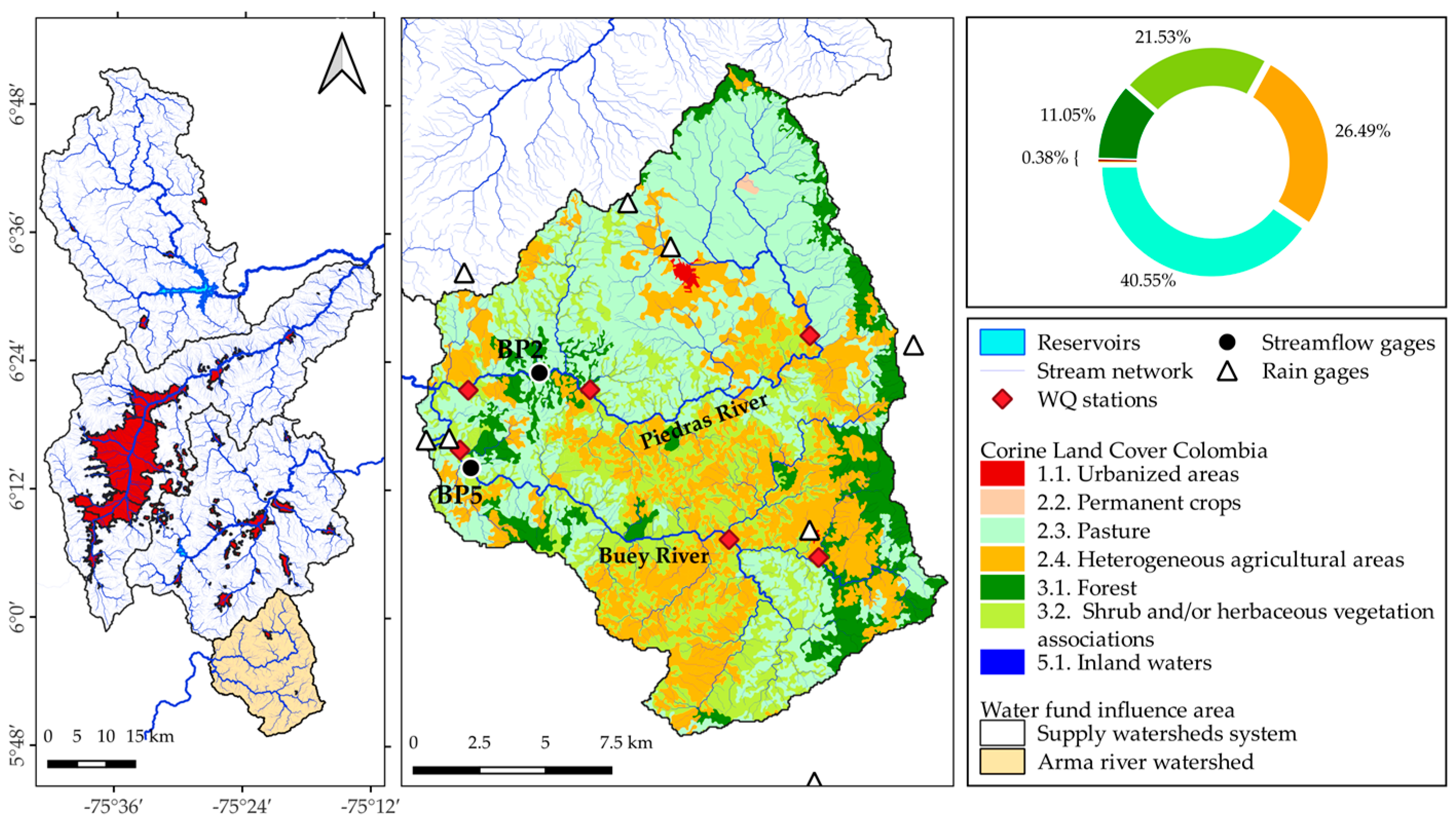
To identify and prioritize relevant management areas for NbS implementations aligned with the WIP goals, we used the mean annual sediment/nutrient delivery from a pixel i to a control or interest point k , δ i k , [15,51] given by:
δ i k = I i j = i + 1 M i k 1 R C j ,
where I i   is the net contribution of sediment/nutrient from element i, R C j is the sediment/nutrient retention coefficient of element j, and M i k is the number of elements (pixels) connecting element i to control point k. It is worth noting that each pixel of the drainage network was considered as a control point, taking into account the relevance of all water bodies in the influence area of the WIP.
In the SIGA-CALv1.0 conceptualization, the net contribution of sediments/nutrients is related to the slope of the terrain (S%), the RUSLE soil erodibility factor (RUSLE-K), direct surface runoff (q), the RUSLE-C coverage factor, and the nonpoint pollutant loads, the last two being directly related to the LULC category. Therefore, considering that the mitigation of sediment/nutrient deliveries through the drainage network by WIP interventions is achieved through NbS (i.e., through the transformation of LULC according to the intervention portfolio described in Section 2.5), Equation (1) can be modified to estimate the average annual delivery of sediments/nutrients that can be avoided, δ i k * , from an element I, as follows:
δ i k * I i B L I i I j = 1 M i k 1 R C j ,
where I i B L   is the net contribution of sediment/nutrient from element i for the baseline simulation scenario, and I i P   is the net contribution of sediment/nutrient from element i for the potential intervention scenario. It must be noted that Equation (2) is presented as an aproximation as I i P   can vary not only in response to LULC changes in pixel i but also due to effects associated with changes upstream.
Since NbS are implemented at the parcel scale, an additional step in the prioritization process requires aggregating the metric δ i k * at this scale as illustrated in Figure 3, where those pixels (within each parcel) with restoration potential contribute by decreasing downhill nitrogen ( δ i N * ), phosphorus ( δ i P * ), total coliforms ( δ i E C * ) and sediment ( δ i T S S * ) loads, and by increasing expected water movements in the soil column which contribute to base flow ( δ i B F * ). Within these calculations, contributions from each variable were normalized in the range [0, 1] and weighted by w -factors equally assigned.
δ p a r c e l * = w S S T P a r c e l δ i T S S * + w N P a r c e l δ i N * + w P P a r c e l δ i P * + w E C P a r c e l δ i E C * + w F B P a r c e l δ i B F *

2.6. Basin of Study

The Arma watershed drains 298.5 km2 at the confluence of the Buey and Piedras rivers (see Figure 4), and accounts for 8.5% of the entire influence area of the CuencaVerde WIP, which is supported by several private and public organizations. The primary objective of the WIP is to enhance water governance, ensure water security, and promote climate change adaptability within the large watershed system that supplies drinking water to one of the most populous metropolitan areas in Colombia [52]. This watershed is in the Magdalena River basin, one of the main water courses in Colombia, and ranges in elevation from 1817 to 2921 m above mean sea level, with average annual precipitation of 2949 mm. The main land uses, according to the CORINE Land Cover types, are pasture (40.55%), heterogeneous agricultural areas (26.49%), shrub and/or herbaceous vegetation (21.53%) and forest (11.05%). Furthermore, the analysis conducted by CuencaVerde using LULC maps from the period 2015–2020 has revealed a significant trend towards increased degradation in the watershed, particularly in the expansion of pasture areas [52].

2.7. Model Input Data

The primary data used to perform the modeling framework with SIGA-CALv1.0 came from the monitoring program carried out in the study area by Empresas Públicas de Medellín, the main partner and funding source for CuencaVerde. Water quality determinants and suspended sediment concentrations are available over the period 2012–2021 for the downstream distributed sites in high (H), medium (M), and low (L) watercourse positions (shown in Figure 4 as WQ—Water Quality—stations) along both the Buey and the Piedras rivers. Daily precipitation and discharge gauge stations are spatially distributed as shown in Figure 4 with records available in the period 2015–2022. Furthermore, daily meteorological data such as solar radiation, temperature, relative humidity, and wind speed/direction were collected from the National Hydrological Center of Colombia IDEAM.
The input data required to perform the modeling framework are presented in detail in the Supplementary Material S3 and summarized in Table 5. An ALOS-PALSAR [53] Digital Elevation Model (DEM) was resampled to a 100 m pixel size to appropriately balance process representativity and computational efficiency [54,55]; this was then used to derive the topological watershed representation as previously described in Section 2.2. Soil layer vector data (1:25,000 scale) obtained from regional agencies [56] were the starting point to obtain the RUSLE K-factor as well as to size the upper soil storage tank within the hydrological model. CORINE Land Cover level three categories were obtained from the 2018 land use cover in the watershed [56], and used to calculate the RUSLE C-factor in line with the European level assessment [57,58] and the Blue Energy Mechanism implemented in two different watersheds use for hydropower in Colombia [47]. To represent the magnitude and variability of the LAI associated with each LULC category, data captured by the NASA MODIS (Moderate Resolution Imaging Spectroradiometer) sensor were used, specifically version 006 of the MCD15A3H product [59] as well as the quality layer FparLai_QC.
Given the lack of survey data at the field scale, nonpoint loads for nitrogen, phosphorus, and total coliforms were assigned based on the LULC classes in the watershed, taking into account available published information of load values per hectare and per year [60]. The information used for each LULC in the modeling exercise can be found in the Supplementary Material S4.

2.8. Model Calibration and Validation

SIGA-CALv1.0 does not have an automatic calibration module. Instead, a semi-automatic and supervised calibration procedure was carried out following a sequential calibration for landcover phenology, streamflow, sediments, and water quality. Most parameters are set regionally by a calibration or correction factor [19], which amplifies or reduces the spatialized parameter baseline values obtained from the input data. This makes the set-up phase highly sensitive and therefore underscores the importance of collecting representative spatial data. Table 6 refers the set of calibration factors corresponding to each of SIGA-CALv1.0′s models.
To calibrate streamflow the discharge record at the BP-2 stream gauge (see Figure 4) was split to enable calibration during the period 2018–2021 and a temporal validation for the period 2015–2018. This calibration was conducted using Monte Carlo simulations, with the first year of data utilized as a warm-up period. Model performance was assessed using the Nash-Sutcliffe efficiency (NSE), and water storage in the lower tanks (tank 3 and tank 4) was supervised to avoid continuous water accumulation. This supervising measure was implemented to prevent long-term simulation trends in streamflow, which can occur even with well-performing parameter sets (NSE > 0.5) due to equifinality issues. CuencaVerde’s special interest in streamflow regulation in relation to NbS implementations necessitated special attention being paid to this component.
In contrast with streamflow, sediment and water quality data are available only for periodic surveys carried out twice a year. Therefore, calibration was performed by comparing and minimizing the deviations between the observed and simulated samples for those specific surveyed days at high (H), medium (M), and low (L) watercourse positions along the Piedras River, for the entire calibration period. A t-test to compare simulations and observations was used as a performance criterion. A spatial validation was performed for the water quality stations along the Buey River.
Since Monte Carlo simulations were performed for both streamflow and water quality, parameter sensitivity was assessed from dot plots for the relationship between objective functions and the corresponding parameter values across the entire Monte Carlo run [61]. The GLUE (Generalized Likelihood Uncertainty Estimation) method was employed to estimate confidence intervals at the 95% level [62,63]. Refer to Supplementary Material S5 for further detail.

3. Results and Discussion

3.1. NbS Spatial Allocation

The spatial distribution of the potential portfolio of NbS implementations is shown in Figure 5. NbS interventions that maximize the L A I parameter to promote the best possible water quality outcomes were chosen. It is worth mentioning that selecting interventions based on shorter establishment times resulted in only marginal outcomes. Nonetheless, given the relevance of establishment time in performing simulations to assess the expected outcomes of NbS interventions, we encourage WIPs and stakeholders to promote monitoring LULC temporal evolution in those areas where NbS are implemented for future analyses.
For the specific portfolio obtained, NbS with higher implementation potential include best livestock practices, conservation, and passive restoration; this reflects current practices being implemented by CuencaVerde in its area of influence. More active strategies, such as nucleation and enrichment planting, which had previously been implemented less due to the lack of surrounding patches with high functional vegetation density, are also recommended.

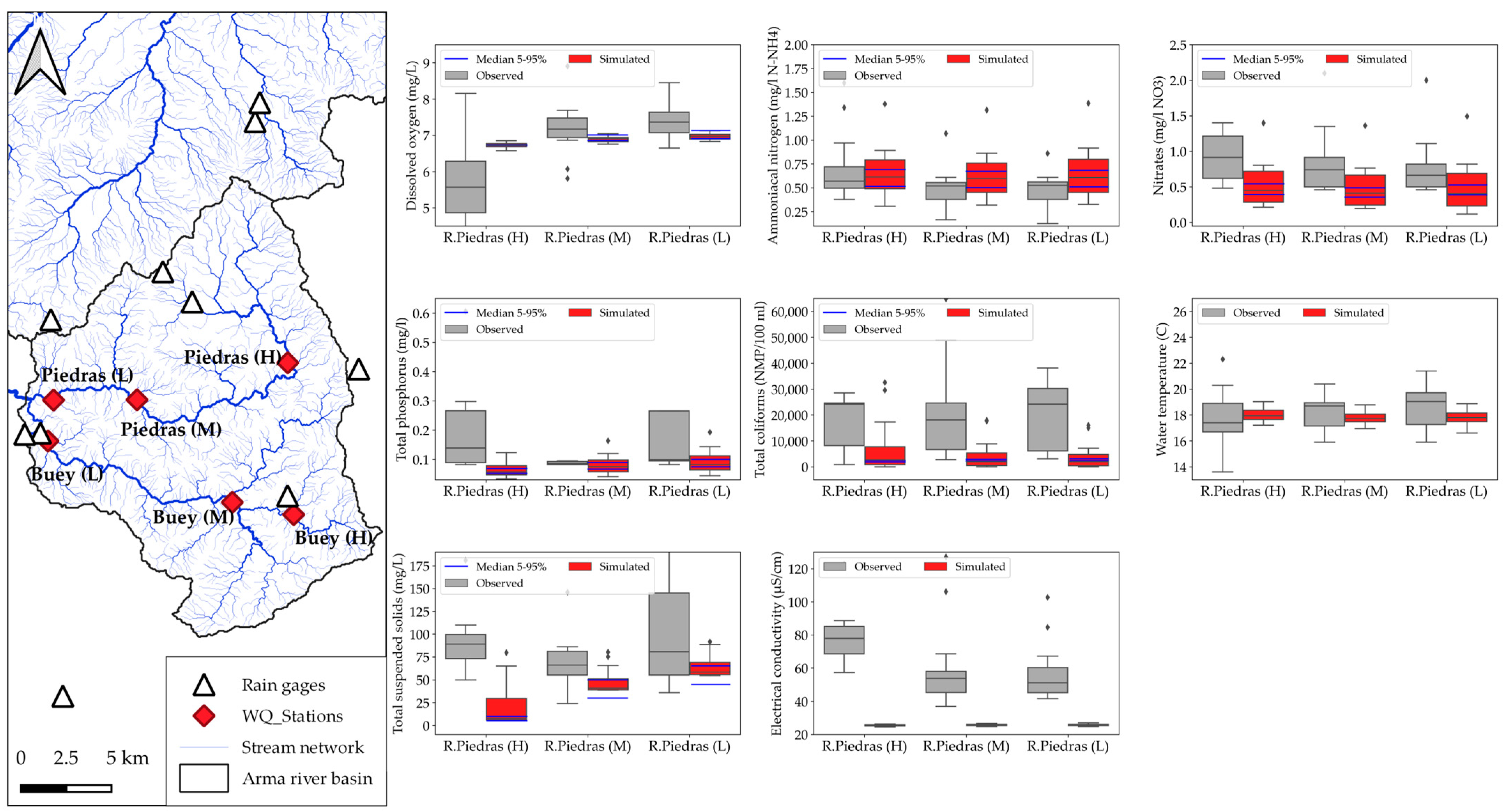
3.2. SIGA-CALv1.0 Calibration

The phenological model was calibrated for CLC classes at level two since level three categories did not allow for the filtering of a representative spatial sample within the study area. Figure 6 shows the calibrated times series in the period 2003–2018 against the MODIS filtered data. Except for permanent crop (CLC class 22), the remaining level two CLC classes have an NSE higher than 35%, reaching values of 54% for pastures (CLC class 23). The poor statistical performance for permanent crops is mainly due to the lack of data as only five cells were found for this CLC class within the basin. It should be noted that, for all coverages, calibration was made using 1-year warming periods.
An additional aspect to highlight in the simulated series in Figure 6 is the fact that they not only adequately represent the oscillations for the CLC classes, but also exhibit variability between different series minima and maxima, demonstrating how the model captures the variability present in the MODIS series. The set of calibrated parameters can be found in Supplementary Material S6.
Figure 7 shows the simulated streamflow after the calibration procedure, for which the performance criteria was close to 50% for both the calibration (2018–2021) and the validation periods (2015–2018). The corresponding baseflow simulation is also shown.
Also shown are the water storages ( S 0 to S 4 ), which were also supervised during the calibration process to avoid any long-term trends, which would have negatively affected model usability for long-term simulations. Instead, we found a pattern for those variables after calibration, which is aligned with the rainfall regime that acts as the main input of water into the basin. Despite the spatial validation at the BP5 stream gage reflecting a reduction in model performance (35.2%), streamflow simulation exhibits consistency for medium and low discharge magnitudes when compared with observations. Deviations for the higher values are due to both the inherent uncertainty structure and temporal resolution of the model, and the fact that the rain gauge network available does not capture storm events, which are likely to explain some extreme discharge events observed in the BP5 record.
Box plots for observed and simulated values of water quality determinants are shown in Figure 8 and Figure 9 for the rivers Buey and Piedras, respectively. The concentration of most determinants is within the same magnitude as the observed data; however, the primary limitation of the simulation lies in the simulated variability. Simulated mean values for dissolved oxygen tend to be lower than observed values; this is likely controlled by the saturation threshold in the model since it is not a variable subject to calibration even if reaeration rate rises. Electrical conductivity, assigned in the model as diffuse contributions from hillslopes, led to simulated values of similar magnitude to the mean observed values along the Buey river. However, the absence of data on point source pollution in urbanized upstream areas of the Piedras river basin may have contributed to significant deviations along this watercourse, for which observed data also show a downstream concentration decline due to assimilation through dilution. Total phosphorus, obtained from the inorganic and organic simulated contributions, as well as nitrates, also tend to be lower than observed values, but this case is more likely related to laboratory detection limits, which truncate the reported values used as observed data. Water temperature and total coliforms simulations perform well for high (H) and medium (M) sites, but they exhibit more notable deviations in the lowland (L) sites. Conversely, total suspended sediment exhibits higher deviations for the high (H) monitoring sites but simulated and observed box plots are closer in the other sites. The total suspended sediments variable was also used to make regional comparisons with the long-term sediment yield at different monitoring sites located in the same hydrological province from the National Hydrological Center network [64]. Figure 10 shows this result, where it is clear that the mean estimations along the control points in the basin follow the expected regional trend using the watershed area as the scaling factor.
It is worth noting that the current SIGA-CALv1.0 structure is based on calibration factors that modify the entire simulation area, but local deviations arising from factors such as input data uncertainty and spatial resolution limitations can limit the effectiveness of this calibration procedure. To overcome this limitation, some distributed models adjust parameters within specific focus areas when results do not align well with the entire region.

3.3. Priority Management Areas

To achieve relevant and achievable outcomes linked to the NbS portfolio suggested in Section 3.1, the metric δ p a r c e l * was obtained using the calibrated model and the configuration of two primary scenarios. First, a baseline scenario was set, based on the most recent CLC map available (year 2020) [65]. Next, a full-intervention scenario was considered, corresponding to the CLC that could be achieved if the entire potential NbS portfolio is implemented throughout the basin, using the information on LULC transitions associated with NbS implementation presented in Table 4. Figure 11a shows the priority order of parcels for NbS implementation by the WIP, with each parcel being assigned a value according to the metric δ p a r c e l * to reflect its relative importance for achieving water objectives. The purpose of this prioritization analysis is to support CuencaVerde’s future decision making regarding NbS interventions (e.g., where to intervene). However, it must be noted that this prioritization is based solely on biophysical analysis of water outcomes; additional WIP objectives, such as biodiversity protection, greenhouse gas sequestration, and socioeconomic improvement may also influence prioritization in practice.
Figure 11b shows both cumulative and avoided loads for nitrogen, phosphorus, and suspended solids, as well as the contributions to baseflow resulting from NbS implementations. The cumulative value given by Equation (2) is also shown, which suggests that, as NbS is implemented in more parcels (area), the expected responses improve naturally. However, the slope of the curve gradually becomes smoother as the restored area increases reaching a threshold area denoted as A * . This suggests the existence of an implementation limit beyond which additional implementations deliver marginal outcomes. This pattern could give insights regarding WIPs’ goals definition regarding primary services related with water quantity and quality (notwithstanding WIPs’ broader objectives as noted above).

3.4. NbS Intermediate Scenarios and Metrics Evaluation

One of the focal points of our work involved simulating baseflow to assess the flow regulation resulting from on-surface NbS implementations. Given the explicit representation of such a process, a direct baseflow estimation is obtained instead using a baseflow separation technique as a surrogate. The baseflow index ( B F I ) suggested by [66] and given by Equation (4) is proposed for aggregating this variable into a single value to make comparisons between simulation scenarios.
B F I = 1 N T Q B Q
The estimated annual mean load at basin outlet, which is determined by Equation (5), was used for nitrogen, phosphorus, and total suspended solids. In this equation, Q t represents the simulated daily mean flow; c t represents the daily mean concentration of nitrogen, phosphorus, or total suspended solids; and N represents the number of simulated days within the simulation period, T. For total coliforms, the annual mean value of the simulated number of individuals was used. These metrics align with the WIP’s (CuencaVerde) monitoring and evaluation plan.
W = 1 N T Q t c t
In addition to the baseline and full-intervention scenarios, three intermediate simulation scenarios were configured representing different percentages of NbS intervention area (i.e., the percentage of the total area of interest to have NbS implemented in it), based on the parcel-scale prioritization. This scenario evaluation is similar to the approach used by [67] to assess the impact of NbS on baseflow and sediment load in the Pipiripau River basin in Brazil, using the SWAT model. The intermediate scenarios correspond to 20%, 50%, and 80% of the potential area being intervened in, as illustrated in Figure 12. These percentages were established based on the cumulative δ p a r c e l * approach to define representative values both above and below the threshold A * .
Water quality and quantity metrics for the intermediate scenarios as well as for the reference baseline and full-intervention scenarios are shown in Figure 13. Results suggest only marginal changes in baseflow, with a slight decrease despite the increase in evapotranspiration rates due to improvements in vegetation cover (greater interception and transpiration). This outcome implies a general maintenance of baseflow despite the additional water losses through evapotranspiration, as also found by [68] who showed, using both SWAT and HEC-HMS simulations, that NbS implementation contributes toward promoting water recharge.
Our modelled findings are also similar to studies conducted by [8] using data from 312 watersheds worldwide, and with the compilation of published data regarding associations between land cover and hydrological metrics conducted by [69], which, in general terms, suggest an increase in the average streamflow as degradation (deforestation) in a watershed vegetation cover occurs and a decrease in this hydrological metric as vegetation cover improves (reforestation). This is shown in Figure 13 for the different intervention scenarios defined. It is worth noting that the observed trend in the average streamflow showed, as shown in Figure 13, is a consequence of the reduction in both the average annual maximum and minimum flows obtained from our daily simulations. The work by [8] also highlights that the response of annual mean streamflow to land cover changes (reforestation or deforestation) is determined not only by the magnitude of the land cover change but also by the climatological properties of each watershed, its flow regime, and the type of forest. Additionally, the work by [8] found that watersheds exhibiting higher sensitivity of annual mean streamflow to land cover change (whether reforestation or deforestation) are those characterized by a higher potential evapotranspiration to precipitation ratio. According to the National Water Study [64], the watershed analyzed herein is in regions with moderate to high water excess, which could also explain the small changes observed in the hydrological assessment metrics for the scenarios.
In contrast to water yield, there is a clear decline in nonpoint loads contributions as the implemented area increases, particularly in the case of total suspended solids and nitrogen. However, as anticipated by the cumulative form of the metric δ p a r c e l * , full NbS intervention in the watershed is not necessarily required to achieve a significant reduction in load contributions to the basin outlet, due to decreasing marginal improvements per additional intervention at higher intervention percentages. This finding highlights the advantage of supporting WIPs with modeling strategies that enable stakeholders to establish relevant intervention goals in terms of expected water services.
The results obtained in the Arma River basin under the full-intervention scenario (100%) (see Figure 13), show that a significant reduction is achieved in different water quality determinants: 47% in sediments, 62% in nitrogen, 8% in phosphorus and 15% in total coliforms. Figure 13 shows how, as the level of NbS intervention in the basin increases, the reduction of these indicators stabilizes, reaching an asymptotic point. This means that, given some economic constraint (total investment amount), an optimal level of NbS intervention to achieve the maximum benefit can be found. In the specific case of the Arma River basin, this optimal intervention point is in a range between 50% and 80% of the whole area that can be implemented through NbS. Within this range, the water quality and quantity objectives proposed for the basin are satisfactorily met. The estimated reductions in this range are between 18.7% and 37.9% in sediments; 45.1% and 59.2% in nitrogen; 6.4% and 7.9% in phosphorus; and 12.3% and 14.6% in total coliforms. It should be noted that the approximation given by the threshold area A * , represents 47% of the NbS portfolio.
In addition, it is necessary to further characterize the diffuse loads applied to the hillslopes due to the sensitivity of nutrients and total coliforms to them during model fitting. This would allow for a more complete understanding of these loads, allowing the decoupling of their estimation from their definition only in terms of LULC classes.
These results contribute to informed decisions on watershed management in the Arma river basin WIP.

4. Conclusions

This paper describes the SIGA-CALv1.0 tool and its underlying modeling framework. The distributed structure of the tool, based on pixels, and the daily temporal scale of its processes, enable the configuration of simulation scenarios, which can be used by decision-makers to define watershed investment programs guided by SMART objectives. Specific nature-based solutions were defined as a function of the expected land cover transformation, and spatially allocated based on decision rules derived from changes in L A I (Leaf-Area Index) and T (establishment time). The extent of the intervened area and the spatial prioritization for NbS intervention (relevant and achievable objectives) were determined using the tool’s results for the baseline and the full-intervention scenarios. Furthermore, the SIGA-CALv1.0 tool allows the obtention of measurable water quantity and quality indicators aligned with WIP monitoring programs or other intervention mechanisms.
It is worth noting that the strategy used to determine the priority order of parcels for NbS intervention within SIGA-CALv1.0 is based on the expected effects on the watershed in terms of a range of water quantity and quality variables. WIPs may in practice also consider other factors related to different ecosystem benefits such as greenhouse gas sequestration, landscape connectivity improvement, or increased biodiversity, which are of interest to certain stakeholders and funders.
Although the overall simulation settings here presented were temporally stationary, SIGA-CALv1.0 is also capable of assessing temporal trends in water quantity and water quality while considering external factors such as new river water diversion, point waste loads (either legally or not legally constituted) and LULC changes as deforestation and expansion of intensive livestock operations.
Further improvements to the tool are a future priority. The supervised calibration process is time-consuming and should be standardized across the tool’s models. Moreover, SIGA-CAL v1.0 should allow for local calibration to overcome deviations driven by input data uncertainty, data scarcity, or spatial resolution. Additionally, the availability of monitoring networks for essential variables such as precipitation is not always guaranteed; therefore, it may be worthwhile incorporating remote sensing products as input data. Improvements are currently underway: for example, enhancements are being made to SIGA-CAL v1.0’s water quality model to enable the inclusion of monitoring stations as boundary conditions to compensate for the lack of data on point source loads that have not necessarily been identified in the territory (e.g., by the corresponding environmental agencies).

Supplementary Materials

The following supporting information can be downloaded at: https://www.mdpi.com/article/10.3390/w15193388/s1, Document S1: Mathematical Description of SIGA-CALv1.0; Document S2: Empirical relations; Document S3: SIGA-CALv1.0 input data required; Document S4: Loads by land use/land cover; Document S5: Uncertainty analysis; Document S6: Calibrated parameters. References [10,18,19,22,25,26,27,29,30,31,32,33,34,35,36,38,41,42,43,46,63,70,71,72,73,74,75,76,77,78,79,80,81,82,83,84,85,86,87,88,89,90,91,92,93,94,95,96,97,98,99,100] are cited in the Supplementary Materials.

Author Contributions

Conceptualization, M.J., C.U., D.P. and J.R.; methodology and analysis, M.J., C.U., D.P. and J.R.; software, C.U., D.P., J.R. and M.J.; writing—original draft preparation, M.J. and C.U.; writing—review and editing, C.AR., E.S.-L. and J.N.; funding acquisition, C.A.R., J.N. and E.S.-L.; supervision, C.A.R. and J.N.; Supplementary Materials, C.A.R. and J.N. All authors have read and agreed to the published version of the manuscript.

Funding

Funding to carry out this work came from the Nature for Water Facility and The Nature Conservancy to enhance a previous version of the tool performed by Gotta Ingeniería S.A.S. as a part of its innovation program to support consultancy projects.

Data Availability Statement

Data available on request due to privacy restrictions.

Acknowledgments

We want to thank the Nature for Water Facility and the CuencaVerde Water Fund for making the project possible. We also thank the environmental agencies CORANTIOQUIA, CORNARE and Area Metropolitana del Valle de Aburrá for providing regional data regarding water diversions and water quality monitoring. We would like to thank Empresas Públicas de Medellín for allowing access to its hydrometeorological data, which is strategic to set the model typology here presented. Finally, we would like to express our gratitude to all those who have previously contributed to the conceptualization of physical processes and the creation of the mathematical model but were not part of the writing of this paper: Juan Pablo Rendón Álvarez, Juanita Cuevas Moreno, Santiago Ospina Leal, Luis Miguel Ruiz, Julián Fernando Yepes Daza, Sandra Patricia Salamanca Jiménez, Carlos Augusto Restrepo Tamayo and Mónica Andrea Bonilla.

Conflicts of Interest

The authors declare no conflict of interest.

References

  1. Ruangpan, L.; Vojinovic, Z.; Di Sabatino, S.; Leo, L.S.; Capobianco, V.; Oen, A.M.P.; McClain, M.E.; Lopez-Gunn, E. Nature-Based Solutions for Hydro-Meteorological Risk Reduction: A State-of-the-Art Review of the Research Area. Nat. Hazards Earth Syst. Sci. 2020, 20, 243–270. [Google Scholar] [CrossRef]
  2. Mosquera-Romero, S.; Ntagia, E.; Rousseau, D.P.L.; Esteve-Núñez, A.; Prévoteau, A. Water Treatment and Reclamation by Implementing Electrochemical Systems with Constructed Wetlands. Environ. Sci. Ecotechnol. 2023, 16, 100265. [Google Scholar] [CrossRef] [PubMed]
  3. Vörösmarty, C.J.; Stewart-Koster, B.; Green, P.A.; Boone, E.L.; Flörke, M.; Fischer, G.; Wiberg, D.A.; Bunn, S.E.; Bhaduri, A.; McIntyre, P.B.; et al. A Green-Gray Path to Global Water Security and Sustainable Infrastructure. Glob. Environ. Chang. 2021, 70, 102344. [Google Scholar] [CrossRef]
  4. Di Grazia, F.; Gumiero, B.; Galgani, L.; Troiani, E.; Ferri, M.; Loiselle, S.A. Ecosystem Services Evaluation of Nature-Based Solutions with the Help of Citizen Scientists. Sustainability 2021, 13, 10629. [Google Scholar] [CrossRef]
  5. Baustian, M.M.; Jung, H.; Bienn, H.C.; Barra, M.; Hemmerling, S.A.; Wang, Y.; White, E.; Meselhe, E. Engaging Coastal Community Members about Natural and Nature-Based Solutions to Assess Their Ecosystem Function. Ecol. Eng. 2020, 143, 100015. [Google Scholar] [CrossRef]
  6. Dutta, A.; Torres, A.S.; Vojinovic, Z. Evaluation of Pollutant Removal Efficiency by Small-Scale Nature-Based Solutions Focusing on Bio-Retention Cells, Vegetative Swale and Porous Pavement. Water 2021, 13, 2361. [Google Scholar] [CrossRef]
  7. Vigerstol, K.L.; Aukema, J.E. A Comparison of Tools for Modeling Freshwater Ecosystem Services. J. Environ. Manag. 2011, 92, 2403–2409. [Google Scholar] [CrossRef]
  8. Zhang, M.; Liu, N.; Harper, R.; Li, Q.; Liu, K.; Wei, X.; Ning, D.; Hou, Y.; Liu, S. A Global Review on Hydrological Responses to Forest Change across Multiple Spatial Scales: Importance of Scale, Climate, Forest Type and Hydrological Regime. J. Hydrol. 2017, 546, 44–59. [Google Scholar] [CrossRef]
  9. Bremer, L.L.; Auerbach, D.A.; Goldstein, J.H.; Vogl, A.L.; Shemie, D.; Kroeger, T.; Nelson, J.L.; Benítez, S.P.; Calvache, A.; Guimarães, J.; et al. One Size Does Not Fit All: Natural Infrastructure Investments within the Latin American Water Funds Partnership. Ecosyst. Serv. 2016, 17, 217–236. [Google Scholar] [CrossRef]
  10. Arnold, J.G.; Srinivasan, R.; Muttiah, R.S.; Williams, J.R. Large Area Hydrologic Modeling and Assessment Part I: Model Development 1. J. Am. Water Resour. Assoc. 1998, 34, 73–89. [Google Scholar] [CrossRef]
  11. Tallis, H.T.; Ricketts, T.; Guerry, A.; Wood, S.A.; Sharp, R.; Nelson, E.; Ennaanay, D.; Wolny, S.; Olwero, N.; Vigerstol, K.; et al. InVEST 2.5.3 User′s Guide. The Natural Capital Project; Stanford University: Stanford, CA, USA, 2013. [Google Scholar]
  12. Francesconi, W.; Srinivasan, R.; Pérez-Miñana, E.; Willcock, S.P.; Quintero, M. Using the Soil and Water Assessment Tool (SWAT) to Model Ecosystem Services: A Systematic Review. J. Hydrol. 2016, 535, 625–636. [Google Scholar] [CrossRef]
  13. Ricci, G.F.; Jeong, J.; De Girolamo, A.M.; Gentile, F. Effectiveness and Feasibility of Different Management Practices to Reduce Soil Erosion in an Agricultural Watershed. Land Use Policy 2020, 90, 104306. [Google Scholar] [CrossRef]
  14. Ricci, G.F.; D’Ambrosio, E.; De Girolamo, A.M.; Gentile, F. Efficiency and Feasibility of Best Management Practices to Reduce Nutrient Loads in an Agricultural River Basin. Agric. Water Manag. 2022, 259, 107241. [Google Scholar] [CrossRef]
  15. Chen, L.; Zhong, Y.; Wei, G.; Cai, Y.; Shen, Z. Development of an Integrated Modeling Approach for Identifying Multilevel Non-Point-Source Priority Management Areas at the Watershed Scale. Water Resour. Res. 2014, 50, 4095–4109. [Google Scholar] [CrossRef]
  16. The Nature Conservancy What Is a Water Fund? Available online: https://waterfundstoolbox.org/getting-started/what-is-a-water-fund (accessed on 10 September 2023).
  17. Velásquez, N.; Vélez, J.I.; Álvarez-Villa, O.D.; Salamanca, S.P. Comprehensive Analysis of Hydrological Processes in a Programmable Environment: The Watershed Modeling Framework. Hydrology 2023, 10, 76. [Google Scholar] [CrossRef]
  18. Vélez, J.I. Desarrollo de Un Modelo Hidrológico Conceptual y Distribuido Orientado a La Simulación de Crecidas. Tesis de Doctorado, Universitat Politècnica de València, Valencia, Spain, 2001. [Google Scholar]
  19. Francés, F.; Vélez, J.I.; Vélez, J.J. Split-Parameter Structure for the Automatic Calibration of Distributed Hydrological Models. J. Hydrol. 2007, 332, 226–240. [Google Scholar] [CrossRef]
  20. Krysanova, V.; Müller-Wohlfeil, D.-I.; Becker, A. Development and Test of a Spatially Distributed Hydrological/Water Quality Model for Mesoscale Watersheds. Ecol. Model. 1998, 106, 261–289. [Google Scholar] [CrossRef]
  21. O’Callaghan, J.F.; Mark, D.M. The Extraction of Drainage Networks from Digital Elevation Data. Comput. Vis. Graph. Image Process. 1984, 28, 323–344. [Google Scholar] [CrossRef]
  22. Shepard, D. A Two-Dimensional Interpolation Function for Irregularly-Spaced Data. In Proceedings of the 1968 23rd ACM National Conference, New York, NY, USA, 27–29 August 1968; ACM Press: New York, NY, USA, 1968; pp. 517–524. [Google Scholar]
  23. Galton, F. Regression Towards Mediocrity in Hereditary Stature. J. Anthropol. Inst. Great Br. Irel. 1886, 15, 246. [Google Scholar] [CrossRef]
  24. Shuttleworth, W.J. Evaporation. In Handbook of Hydrology; McGraw-Hill: New York, NY, USA, 1993; Volume 1, pp. 4.1–4.53. [Google Scholar]
  25. Allen, R.G.; Pereira, L.S.; Raes, D.; Smith, M. Crop Evapotranspiration-Guidelines for Computing Crop Water Requirements. Food Agric. Organ. United Nations Rome 1998, 300, D05109. [Google Scholar]
  26. Gómez Elorza, Á. Herramientas de Modelación y Monitoreo Para La Hidrología de Alta Montaña Colombiana—Cuenca de La Quebrada Calostros—PNN Chingaza. Master’s Thesis, Universidad Nacional de Colombia Sede Bogotá, Bogotá, Colombia, 2016. [Google Scholar]
  27. Alemayehu, T.; van Griensven, A.; Woldegiorgis, B.T.; Bauwens, W. An Improved SWAT Vegetation Growth Module and Its Evaluation for Four Tropical Ecosystems. Hydrol. Earth Syst. Sci. 2017, 21, 4449–4467. [Google Scholar] [CrossRef]
  28. Waring, R.H.; Running, S.W. Water Cycle. In Forest Ecosystems; Elsevier: Amsterdam, The Netherlands, 2007; pp. 19–57. [Google Scholar]
  29. Kilinc, M.Y. Mechanics of Soil Erosion from Overland Flow Generated by Simulated Rainfall; Colorado State University: Fort Collins, CO, USA, 1972. [Google Scholar]
  30. Julien, P.Y. Erosion and Sedimentation; Cambridge University Press: Cambridge, UK, 1995; ISBN 9780521442374. [Google Scholar]
  31. Rojas, R.; Julien, P.; Johnson, B. A 2-Dimensional Rainfall-Runoff and Sediment Model; CASC2D-SED Reference Manual v1. 0; Colorado State University: Fort Collins, CO, USA, 2003. [Google Scholar]
  32. Wilkinson, S.N.; Dougall, C.; Kinsey-Henderson, A.E.; Searle, R.D.; Ellis, R.J.; Bartley, R. Development of a Time-Stepping Sediment Budget Model for Assessing Land Use Impacts in Large River Basins. Sci. Total Environ. 2014, 468–469, 1210–1224. [Google Scholar] [CrossRef] [PubMed]
  33. Engelund, F.; Hansen, E. A Monograph on Sediment Transport in Alluvial Streams. 1967. Available online: https://repository.tudelft.nl/islandora/object/uuid%3A81101b08-04b5-4082-9121-861949c336c9 (accessed on 25 September 2023).
  34. Osorio Yepes, S. Simulación de Sedimentos Mediante Un Modelo Hidrológico Distribuido Utilizando Información Indirecta. Master’s Thesis, Universidad Nacional de Colombia Sede Medellín, Medellín, Colombia, 2016. [Google Scholar]
  35. Aristizábal, E.; Vélez, J.I.; Martínez, H.E.; Jaboyedoff, M. SHIA_Landslide: A Distributed Conceptual and Physically Based Model to Forecast the Temporal and Spatial Occurrence of Shallow Landslides Triggered by Rainfall in Tropical and Mountainous Basins. Landslides 2016, 13, 497–517. [Google Scholar] [CrossRef]
  36. Arnone, E.; Noto, L.V.; Lepore, C.; Bras, R.L. Physically-Based and Distributed Approach to Analyze Rainfall-Triggered Landslides at Watershed Scale. Geomorphology 2011, 133, 121–131. [Google Scholar] [CrossRef]
  37. Taylor, D.W. Fundamentals of Soil Mechanics, 1st ed.; Wiley: New York, NY, USA, 1948; Volume 1. [Google Scholar]
  38. Tsai, Z.-X.; You, G.J.-Y.; Lee, H.-Y.; Chiu, Y.-J. Modeling the Sediment Yield from Landslides in the Shihmen Reservoir Watershed, Taiwan. Earth Surf. Process. Landf. 2013, 38, 661–674. [Google Scholar] [CrossRef]
  39. Wade, A.J.; Whitehead, P.G.; Butterfield, D. The Integrated Catchments Model of Phosphorus Dynamics (INCA-P), a New Approach for Multiple Source Assessment in Heterogeneous River Systems: Model Structure and Equations. Hydrol. Earth Syst. Sci. 2002, 6, 583–606. [Google Scholar] [CrossRef]
  40. Wade, A.J.; Durand, P.; Beaujouan, V.; Wessel, W.W.; Raat, K.J.; Whitehead, P.G.; Butterfield, D.; Rankinen, K.; Lepisto, A. A Nitrogen Model for European Catchments: INCA, New Model Structure and Equations. Hydrol. Earth Syst. Sci. 2002, 6, 559–582. [Google Scholar] [CrossRef]
  41. Whitehead, P.G.; Wilson, E.J.; Butterfield, D. A Semi-Distributed Integrated Nitrogen Model for Multiple Source Assessment in Catchments (INCA): Part I—Model Structure and Process Equations. Sci. Total Environ. 1998, 210–211, 547–558. [Google Scholar] [CrossRef]
  42. Vélez, J.; Francés, F.; Vélez, I. TETIS: A Catchment Hydrological Distributed Conceptual Model. Geophys. Res. Abstr. 2005, 7, 03503. [Google Scholar]
  43. Beer, T.; Young, P.C. Longitudinal Dispersion in Natural Streams. J. Environ. Eng. 1983, 109, 1049–1067. [Google Scholar] [CrossRef]
  44. Santos Santos, T.F. Development of an Environmental Multiscale Decision Support System (EMDSS) for Sustainable Water Management in Highly Complex Altered Catchments. Tesis de Doctorado, Universidad de los Andes, Bogotá, Colombia, 2020. [Google Scholar]
  45. Whitehead, P.G.; Williams, R.J.; Lewis, D.R. Quality Simulation along River Systems (QUASAR): Model Theory and Development. Sci. Total Environ. 1997, 194–195, 447–456. [Google Scholar] [CrossRef]
  46. Lees, M.J.; Camacho, L.; Whitehead, P. Extension of the QUASAR River Water Quality Model to Incorporate Dead-Zone Mixing. Hydrol. Earth Syst. Sci. 1998, 2, 353–365. [Google Scholar] [CrossRef]
  47. The Nature Conservancy. Gotta Ingeniería Caracterización y Modelamiento de La Hidrología y Sedimentología de 2 Cuencas Piloto En El Marco Del Proyecto Blue Energy Mechanism (BEM); The Nature Conservancy: Medellín, Colombia, 2021. [Google Scholar]
  48. Bossard, M.; Feranec, J.; Otahel, J. CORINE Land Cover Technical Guide: Addendum 2000; European Environment Agency: Copenhagen, Denmark, 2000; Volume 40. [Google Scholar]
  49. Instituto de Hidrología, Meteorología y Estudios Ambientales (IDEAM). Leyenda Nacional de Coberturas de La Tierra, Metodología Corine Land Cover Para Colombia, Escala 1:100.000; IDEAM: Bogotá, Colombia, 2010. [Google Scholar]
  50. Buytaert, W.; Célleri, R.; De Bièvre, B.; Cisneros, F.; Wyseure, G.; Deckers, J.; Hofstede, R. Human Impact on the Hydrology of the Andean Páramos. Earth-Sci. Rev. 2006, 79, 53–72. [Google Scholar] [CrossRef]
  51. Lu, H.; Moran, C.J.; Prosser, I.P.; DeRose, R. Investment Prioritization Based on Broadscale Spatial Budgeting to Meet Downstream Targets for Suspended Sediment Loads. Water Resour. Res. 2004, 40. [Google Scholar] [CrossRef]
  52. Water Fund CuencaVerde. Available online: https://www.cuencaverde.org/ (accessed on 25 September 2023).
  53. Alaska Satellite Facility Dataset: ASF DAAC 2015, ALOS PALSAR_Radiometric_Terrain_Corrected_high_res; Includes Material © JAXA/METI 2007. Available online: https://search.asf.alaska.edu/#/ (accessed on 25 September 2023).
  54. Rojas, R.; Velleux, M.; Julien, P.Y.; Johnson, B.E. Grid Scale Effects on Watershed Soil Erosion Models. J. Hydrol. Eng. 2008, 13, 793–802. [Google Scholar] [CrossRef]
  55. Sharma, A.; Tiwari, K.N.; Bhadoria, P.B.S. Determining the Optimum Cell Size of Digital Elevation Model for Hydrologic Application. J. Earth Syst. Sci. 2011, 120, 573–582. [Google Scholar] [CrossRef]
  56. Sistema de Información Ambiental de Colombia -SIAC- Catálogo de Mapas SIAC. Available online: www.siac.gov.co/catalogo-de-mapas (accessed on 10 September 2023).
  57. Panagos, P.; Borrelli, P.; Meusburger, K.; Alewell, C.; Lugato, E.; Montanarella, L. Estimating the Soil Erosion Cover-Management Factor at the European Scale. Land Use Policy 2015, 48, 38–50. [Google Scholar] [CrossRef]
  58. Bosco, C.; de Rigo, D. Land Cover and Soil Erodibility within the E-RUSLE Model. Scientific Topics Focus 1, MRI-11b13. Notes Transdiscipl. Model. Env., Maieutike Research Initiative. 2013. Available online: https://figshare.com/articles/dataset/Land_Cover_and_Soil_Erodibility_whithin_the_e_RUSLE_Model/856670/2 (accessed on 10 September 2023).
  59. Myneni, R.; Park, Y. MODIS Collection 6 (C6) LAI/FPAR Product User’s Guide. 2015. Available online: https://lpdaac.usgs.gov/documents/2/mod15_user_guide.pdf (accessed on 10 September 2023).
  60. Salata, S.; Garnero, G.; Barbieri, C.; Giaimo, C. The Integration of Ecosystem Services in Planning: An Evaluation of the Nutrient Retention Model Using InVEST Software. Land 2017, 6, 48. [Google Scholar] [CrossRef]
  61. Ward, A.S.; Kelleher, C.A.; Mason, S.J.K.; Wagener, T.; McIntyre, N.; McGlynn, B.; Runkel, R.L.; Payn, R.A. A Software Tool to Assess Uncertainty in Transient-Storage Model Parameters Using Monte Carlo Simulations. Freshw. Sci. 2017, 36, 195–217. [Google Scholar] [CrossRef]
  62. Xiong, L.; Wan, M.; Wei, X.; O’Connor, K.M. Indices for Assessing the Prediction Bounds of Hydrological Models and Application by Generalised Likelihood Uncertainty Estimation/Indices Pour Évaluer Les Bornes de Prévision de Modèles Hydrologiques et Mise En Œuvre Pour Une Estimation d’incertitude Par Vraisemblance Généralisée. Hydrol. Sci. J. 2009, 54, 852–871. [Google Scholar] [CrossRef]
  63. Beven, K.; Binley, A. The Future of Distributed Models: Model Calibration and Uncertainty Prediction. Hydrol. Process. 1992, 6, 279–298. [Google Scholar] [CrossRef]
  64. Instituto de Hidrología, Meteorología y Estudios Ambientales (IDEAM). Anexos—Estudio Nacional Del Agua. 2022. Available online: http://www.ideam.gov.co/web/agua/estudio-nacional-del-agua (accessed on 10 September 2023).
  65. Water Fund CuencaVerde. Priorización de Áreas de Protección Hídrica en las Cuencas Abastecedoras del Sistema de Abastecimiento de Agua Potable de Empresas Públicas de Medellín; Water Fund CuencaVerde: Medelllín, Colombia, 2022. [Google Scholar]
  66. Razavi, T.; Coulibaly, P. Classification of Ontario Watersheds Based on Physical Attributes and Streamflow Series. J. Hydrol. 2013, 493, 81–94. [Google Scholar] [CrossRef]
  67. Strauch, M.; Lima, J.E.F.W.; Volk, M.; Lorz, C.; Makeschin, F. The Impact of Best Management Practices on Simulated Streamflow and Sediment Load in a Central Brazilian Catchment. J. Environ. Manag. 2013, 127, S24–S36. [Google Scholar] [CrossRef] [PubMed]
  68. Acosta, E.A.; Cho, S.J.; Klemz, C.; Reapple, J.; Barreto, S.; Ciasca, B.S.; León, J.; Rogéliz-Prada, C.A.; Bracale, H. Biophysical Benefits Simulation Modeling Framework for Investments in Nature-Based Solutions in São Paulo, Brazil Water Supply System. Water 2023, 15, 681. [Google Scholar] [CrossRef]
  69. Acreman, M.; Smith, A.; Charters, L.; Tickner, D.; Opperman, J.; Acreman, S.; Edwards, F.; Sayers, P.; Chivava, F. Evidence for the Effectiveness of Nature-Based Solutions to Water Issues in Africa. Environ. Res. Lett. 2021, 16, 063007. [Google Scholar] [CrossRef]
  70. Frei, C. Interpolation of Temperature in a Mountainous Region Using Nonlinear Profiles and Non-Euclidean Distances. Int. J. Climatol. 2014, 34, 1585–1605. [Google Scholar] [CrossRef]
  71. Shuttleworth, W.J. Putting the “Vap” into Evaporation. Hydrol. Earth Syst. Sci. 2007, 11, 210–244. [Google Scholar] [CrossRef]
  72. Tobón, C.; Morales, E.G.G. Capacidad de Interceptación de La Niebla Por La Vegetación de Los Páramos Andinos. Av. Recur. Hidráulicos 2007, 15, 35–46. [Google Scholar]
  73. Gultepe, I.; Isaac, G.A. Liquid Water Content and Temperature Relationship from Aircraft Observations and Its Applicability to GCMs. J. Clim. 1997, 10, 446–452. [Google Scholar] [CrossRef]
  74. Romps, D.M. Exact Expression for the Lifting Condensation Level. J. Atmos. Sci. 2017, 74, 3891–3900. [Google Scholar] [CrossRef]
  75. Neitsch, S.L.; Arnold, J.G.; Kiniry, J.R.; Williams, J.R. Soil and Water Assessment Tool—Theoretical Documentation—Version 2009; Texas Water Resources Institute: College Station, TX, USA, 2011. [Google Scholar]
  76. Francés, F.; Vélez, J.J.; Vélez, J.I.; Puricelli, M. Distributed Modelling of Large Basins for a Real Time Flood Forecasting System in Spain. In Proceedings of the Second Federal Interagency Hydrologic Modelling Conference, Gan, TY and Biftu, Las Vegas, NV, USA, 28 July–1 August 2002; pp. 3513–3524. [Google Scholar]
  77. Restrepo-Tamayo, C.A. Modelo Hidrológico Distribuido Orientado a La Gestión de La Utilización Conjunta de Aguas Superficiales y Subterráneas. Master’s Thesis, Universidad Nacional de Colombia, Sede Medellín, Medellín, Colombia, 2007. [Google Scholar]
  78. Velázquez, N. Simulación de Sedimentos a Partir de Un Modelo Conceptual y Distribuido No Lineal. Master’s Thesis, Facultad de Minas, Universidad Nacional de Colombia, Medellín, Colombia, 2011. [Google Scholar]
  79. Cataño-Álvarez, S.; Vélez-Upegui, J.I. Modelo Conceptual Agregado de Transporte de Sedimentos Para Cuencas de Montaña En Antioquia-Colombia. Boletín Cienc. Tierra 2016, 38–48. [Google Scholar] [CrossRef]
  80. Sáenz, L.L.; Mulligan, M. Análisis Científico Detallado del Impacto del Cambio del Uso del Suelo en el Suministro de Recursos Hídricos Para la Ciudad de Bogotá e Implicaciones Para el Desarrollo de Esquemas PES; Department of Geography, King’s College London: London, UK, 2007. [Google Scholar]
  81. Hofstede, R.; Mondragon, M.; Rocha, C. Biomass of Grazed, Burned, and Undisturbed Paramo Grasslands, Colombia. I. Aboveground Vegetation. Artic Alp. Res. 1995, 27, 1–12. [Google Scholar] [CrossRef]
  82. Buytaert, W.; Célleri, R.; De Bièvre, B.; Cisneros, F. Hidrología del Páramo Andino: Propiedades, Importancia y Vulnerabilidad. 2005. Available online: https://www.researchgate.net/profile/felipe-cisneros/publication/228459137_hidrologia_del_paramo_andino_propiedades_importancia_y_vulnerabilidad/links/0deec528f8f8e65d5e000000/hidrologia-del-paramo-andino-propiedades-importancia-y-vulnerabilidad.pdf (accessed on 10 September 2023).
  83. Mulligan, M.; Torres, E.; Jarvis, A.; González, J.; Sáenz, L.L. Field and Laboratory Measurement of Rates and Processes of Clud Interception by Epiphytes, Leaves and Standard Collectors. In Forests in the Mist: Science for Conserving and Managing Tropical Montane Cloud Forests; Bruijnzeel, L.A., Juvik, J., Scatena, F.N., Hamilton, L.S., Bubb, P., Eds.; University of Hawaii: Honolulu, HI, USA, 2006. [Google Scholar]
  84. Bergström, S. The HBV Model. In Computer Models of Watershed Hydrology; Singh, V.P., Ed.; Water Resources Publications: Littleton, CO, USA, 1995. [Google Scholar]
  85. Arnaud, P.; Lavabre, J. Simulation du Functionnement Hydrologique d’une Retenue d’eau; Cemagref: Paris, France, 1996. [Google Scholar]
  86. Michel, C. Hydrologie Appliquée Aux Petits Bassins Ruraux; Cemagref: Paris, France, 1989. [Google Scholar]
  87. Singh, V.P.; Dickinson, W.T. An Analytical Method to Determine Daily Soil Moisture. In Proceedings of the Second World Congress on Water Resources, Delhi, India, 12–16 December 1975; pp. 355–365. [Google Scholar]
  88. Foster, G.R.; Lane, L.J. Modelling Rill Density. J. Irrig. Drain. Div. Proc. ASCE 1981, 107, 109–112. [Google Scholar] [CrossRef]
  89. Moor, I.D.; Burch, G.J. Sediment Transport Capacity o Sheet and Rill Flow: Application of Unit Stream Power Theory. Water Resour. Res. 1986, 22, 1350–1360. [Google Scholar] [CrossRef]
  90. Parsons, A.J.; Abrahams, A.D.; Wainwright, J. On Determining Resistance to Interrill Overland Flow. Water Resour. Res. 1994, 30, 3515–3521. [Google Scholar] [CrossRef]
  91. Boyd, J.P. Finding the Zeros of a Univariate Equation: Proxy Rootfinders, Chebyshev Interpolation, and the Companion Matrix. SIAM Rev. 2013, 55, 375–396. [Google Scholar] [CrossRef]
  92. Prosser, I.P.; Rustomji, P. Sediment Transport Capacity Relations for Overland Flow. Prog. Phys. Geogr. 2000, 24, 179–193. [Google Scholar] [CrossRef]
  93. Graham, S. Cuphea Fluviatilis (Lythraceae), a New Species from Antioquia, Colombia. Novon 2009, 19, 45–48. [Google Scholar] [CrossRef]
  94. Burton, A.; Bathurst, J.C. Physically Based Modelling of Shallow Landslide Sediment Yield at a Catchment Scale. Environ. Geol. 1998, 35, 89–99. [Google Scholar] [CrossRef]
  95. Bathurst, J.C.; Burton, A.; Ward, T.J. Debris Flow Run-out and Landslide Sediment Delivery Model Tests. J. Hydraul. Eng. 1997, 123, 410–419. [Google Scholar] [CrossRef]
  96. Bowles, D.S. Delineation of Landslide, Flash Flood, and Debris Flow Hazards in Utah. 1985. Available online: https://digitalcommons.usu.edu/water_rep/596/ (accessed on 10 September 2023).
  97. Larsen, M.C. Landslides and Sediment Budgets in Four Watersheds in Eastern Puerto Rico. In Water Quality and Landscape Processes of Four Watersheds in Eastern Puerto Rico; USGS: Reston, VA, USA, 2012; Volume 1789, pp. 153–178. [Google Scholar]
  98. Simonett, D.S.; Jennings, J.N.; Mabbutt, J.A. Landform Studies from Australia and New Guinea; ANU Press: Canberra, Australia, 1967. [Google Scholar]
  99. Lees, M.J.; Camacho, L.A.; Chapra, S. On the Relationship of Transient Storage and Aggregated Dead Zone Models of Longitudinal Solute Transport in Streams. Water Resour. Res. 2000, 36, 213–224. [Google Scholar] [CrossRef]
  100. Foster, G.R.; Huggins, L.F.; Meyer, L.D. A Laboratory Study of Rill Hydraulics: Velocitiy Relationships. Trans. Am. Soc. Agric. Eng. 1984, 25, 940–947. [Google Scholar]
Figure 1. Topological representation of SIGA-CALv1.0 models.
Water 15 03388 g001
Figure 2. Example for the scheme adopted for the allocation of specific NbS actions in the study area, based on (a) the baseline LULC class and the intervention pathway according with the parameters T and L A I , and (b) the score P assigned to each pathway from the normalized quantities T * and L A I * .
Water 15 03388 g002
Figure 3. Schematization of the δ p a r c e l * metric assessment from restored pixels within a parcel.
Water 15 03388 g003
Figure 4. Study area.
Water 15 03388 g004
Figure 5. Allocation of the NbS portfolio within the study area.
Water 15 03388 g005
Figure 6. L A I variability representation for different CLC classes, after the calibration of the phenological SIGA-CALv1.0 model.
Water 15 03388 g006
Figure 7. Streamflow calibration results at BP2 stream gage in the period 2018–2021. Temporal validation is also shown as time series for the period 2015–2018, and spatial validation in BP5 stream gage.
Water 15 03388 g007
Figure 8. Water quality and sediment calibration in high (H), medium (M) and low (L) sites along the Buey river. The upper whisker for box plots is determined by the minimum of either the highest value in the series or the value corresponding to (Q75 + 1.5IQR). Similarly, the lower whisker is determined by the maximum of either the maximum of the series or (Q25 − 1.5IQR). Gray diamonds represent values that are either above or below the upper or lower whisker, respectively.
Water 15 03388 g008
Figure 9. Water quality and sediment calibration in high (H), medium (M) and low (L) sites along the Piedras river. The upper whisker for box plots is determined by the minimum of either the highest value in the series or the value corresponding to (Q75 + 1.5IQR). Similarly, the lower whisker is determined by the maximum of either the maximum of the series or (Q25 − 1.5IQR). Gray diamonds represent values that are either above or below the upper or lower whisker, respectively.
Water 15 03388 g009
Figure 10. Regional comparisons for suspended sediment yield simulations after calibration, with mean values available in monitoring sites in the same hydrological province. Dotted line represents the general trend corresponding to the regional available data.
Water 15 03388 g010
Figure 11. (a) Priority of intervention at the parcel scale, and (b) cumulative avoided deliveries of nitrogen ( δ i N * ), phosphorus ( δ i P * ), total coliforms ( δ i E C * ) and sediment ( δ i T S S * ) loads, and expected water movements in the soil column which contribute to base flow ( δ i B F * ).
Water 15 03388 g011
Figure 12. Intermediate NbS intervention scenarios for analysis.
Water 15 03388 g012
Figure 13. Metrics of water regulation and diffuse pollution loads for NbS intervention scenarios.
Water 15 03388 g013
Table 1. Modeling tools for accounting for water quantity and water quality attributes.
Model AspectModeling Tools
SWATInVESTSIGA-CALv1.0
(This Exercise)
Time stepDailyAnnualDaily
ScaleSubbasinCell-based sizeCell-based size
Water primary serviceWater yield, stream flow, base flow, flood regulation, nitrogen load/concentration, phosphorus load/concentration, sediment load/concentrationWater yield, sediment yield, nutrient yie ldWater yield, stream flow, base flow, flood regulation, nitrogen load/concentration, phosphorus load/concentration, sediment load/concentration, dissolved oxygen, biochemical oxygen demand, pH, pathogen indicators (total coliforms)
Table 2. Linking SMART objectives with the modeling tool SIGA-CALv1.0 capabilities (see Section 2.3).
CriteriaChallengeGoal
SpecificLinking improvements to NbS portfolios with modeled parametrization To define potential NbS interventions based on the actual watershed Land Use/Land Cover (LULC), as well as relating the induced LULC change with hydrological and water quality processes
MeasurableNbS effects take time to materialize, thus monitoring and modeling allow for the assessment of the likely tendency and impact of outcomes in advance To estimate attributes of water quantity and water quality and align them with Water Funds’ practical monitoring and evaluation programs
AchievableWIPs targeting water security issues must define a realistic program(s) of NbS interventions that aim to achieve relevant outcomesTo identify how much NbS to implement based on established goals, and where
RelevantMost WIPs and NbS are voluntary and may thus not deliver optimal interventions, particularly if not targeted preciselyTo identify and prioritize management areas to best achieve the goals of the WIP
Time-boundFew models enable a dynamic simulation of the temporal effects of NbS, which is important for assessing the timing of benefits of water quantity and quality To give WIPs simulation capabilities to assess temporal trends in water quantity and water quality, while considering external factors that may cause deviations from expected outcomes
Table 3. Definition of NbS in SIGA-CALv1.0.
NbSDefinition
Best livestock practicesActive introduction of shrub and tree plants that serve to improve soils and provide fodder for livestock. This is generally associated with an improvement of previously compacted soils, as well as an improvement in pasture quality. About 200 plants are used for each single hectare of a system with best livestock practices. These plants are arranged linearly every 3 m along the boundaries of the property, or to separate paddocks.
Best agricultural practicesActive introduction of productive plants, usually shrubs or trees, often in combination with other species. Arrangements that contribute to greater productivity, such as live fences, are also often incorporated. For each single hectare of a system with best agricultural practices about 200 plants are used. These plants are dispersed throughout the property depending on drainage conditions, slope, and soil type. They can also be arranged as a corridor at the boundaries of the property.
NucleationA combination of actions aimed to aid the recovery of vegetative cover. Nucleation consists of installing cores of native plants that attract dispersers and facilitate natural regeneration. It should only be implemented in areas adjacent to natural areas. Nucleation requires planting approximately 800 trees per hectare.
Enrichment plantingA combination of actions aimed to aid the recovery of vegetative cover. Active restoration by enrichment planting consists of introducing native plants in the most degraded parts of an area where there are already traces of native vegetation. This approach requires the planting of approximately 390 trees per hectare.
Passive restorationA combination of actions that facilitates the natural regeneration of vegetation. These actions are mainly aimed at removing the source of degradation of vegetative cover—the most common strategy is physical fencing (e.g., spike or electric fencing) to protect areas. Some passive restoration exercises also include installing structures that serve as perches or shelters for animals that are potential seed dispersers to attract them and expedite the process. No planting is carried out in this scheme.
Table 4. LULC class transitions for the specific NbS portfolio represented in SIGA-CALv1.0.
NbSBase
LULC
Base
LULC Code
Final
LULC
Final LULC
Code
T
(Years)
L A I
Best livestock practicesMosaic of pastures and crops242Mosaic of crops, pastures, and natural areas243100
Wooded pastures232Mosaic of pastures with natural spaces24470.56
Weedy pastures233Mosaic of pastures with natural spaces244100.56
Clean pastures231Mosaic of pastures with natural spaces244120.56
Bare and degraded lands333Mosaic of pastures with natural spaces244132.89
Best agricultural practicesPermanent shrub crops222Mosaic of crops and natural spaces245100.6
Permanent herbaceous crops221Mosaic of crops and natural spaces245100.6
Crop mosaic241Mosaic of crops and natural spaces245120
Pasture and crop mosaic242Mosaic of pastures and crops243100
Other transitory crops211Mosaic of crops and natural spaces245120.6
Tubers215Mosaic of crops and natural spaces245120.6
NucleationWeeded pastures233Fragmented forest313190.82
Weeded pastures233Grassland321191.01
Clean pasture231Fragmented forest313210.82
Clean pasture231Grassland321211.01
Bare and degraded land333Secondary or transitional vegetation323221.72
Enrichment plantingOpen forest312Dense forest311190
Fragmented forest313Open forest312110
Mosaic of pastures with natural spaces244Fragmented forest313140.26
Wooded pasture232Open forest312160.82
Wooded pasture232Grassland321161.01
Secondary or transitional vegetation323Open forest31219−0.19
Passive
restoration
Open forest312Dense forest311190
Fragmented forest313Open forest312190
Mosaic of pastures with natural spaces244Secondary or transitional vegetation323220
Secondary or transitional vegetation323Fragmented forest31327−0.19
Table 5. Input data to SIGA-CALv1.0 modeling framework.
Data FormatDescription
RasterDigital Elevation Model
Flow direction map
Flow accumulation map
Sand, silt and clay fraction in soil
Soil depth and organic matter fraction
Soil cohesion and angle of repose
RUSLE erodibility and cropping practice factors
Subterranean water interchange rate
Paramo areas
Level 3 CORINE LULC map
Integer id representing nitrogen, phosphorus and total coliforms loads and their annual variations
Environmental flow demand map
Integer code representing a LULC transition from a base line to a desired final state according to the NbS portfolio
Integer code representing the NbS intervention priority of each pixel
VectorParcel of land owned by a single person or entity in the watershed
Text fileWater diversions
Point waste loads
Table 6. Main SIGA-CALv1.0 parameters for calibration.
ProcessCalibration Factors Description
Phenological model aMaximum and minimum L A I for each CLC class represented
Total heat units required for plant maturity
Fraction of heat units accumulated on a given date
Soil humidity contents factors
Temperature limits that contribute to vegetative development
Hydrological modelVertical precipitation depth
Horizontal precipitation depth
Maximum leaf storage
Maximum capillary storage
Maximum gravitational storage
Subsurface permeability
Groundwater permeability
Subsurface exchange permeability
Hillslope flow velocity
Subsurface flow velocity
Groundwater flow velocity
Instream flow velocity
Sedimentological modelHillslope sediment transport capacity
Stream sediment transport capacity
Bank erosion
Sediment supply disaggregation factor
Landslide modelSoil cohesion and friction angle
Water qualityBDOOxidation rate
DOReaeration model
Reaeration factor
Nitrogen formsNitrogen load factor on hillslopes
Plant nitrogen uptake rates
Nitrification rates from organic nitrogen to nitrites
Nitrogen forms settling velocity
Phosphorus formsPhosphorus load factor on hillslopes
Phosphorus mineralization rates
Phosphorus immobilization rate
Plant phosphorus uptake rate
Organic/Inorganic phosphorus sorption
Organic phosphorus hydrolysis
Phosphorus forms settling velocity
Total coliformsTotal coliforms load factor on hillslopes
Growth and die-off bacteria ratesSediment fraction adsorption
TemperatureTemperature correction factors
Note: a Calibrated parameters are absolute quantities instead of correction factors.
Disclaimer/Publisher’s Note: The statements, opinions and data contained in all publications are solely those of the individual author(s) and contributor(s) and not of MDPI and/or the editor(s). MDPI and/or the editor(s) disclaim responsibility for any injury to people or property resulting from any ideas, methods, instructions or products referred to in the content.

