
Significant Daily CO2 Source–Sink Interchange in an Urbanizing Lake in Southwest China
by
 ,
,
Rongjie Yang
1,2, 
Yingying Chen
2,
Di Li
2,3,
Yuling Qiu
2,
Kezhu Lu
2,
Shiliang Liu
2,4,* and
Huixing Song
2,* 1
School of Tourism and Culture Industry, Chengdu University, Chengdu 610106, China
2
College of Landscape Architecture, Sichuan Agricultural University, Chengdu 611130, China
3
Brigade of Physical Exploration, Hubei Geological Bureau, Wuhan 430100, China
4
Sichuan Yuze (Xscape) Landscape Planning and Design Co., Ltd., Chengdu 610093, China
*
Authors to whom correspondence should be addressed.
Water 2023, 15(19), 3365; https://doi.org/10.3390/w15193365
Submission received: 7 August 2023
/
Revised: 15 September 2023
/
Accepted: 23 September 2023
/
Published: 25 September 2023
(This article belongs to the Special Issue Wetland Ecosystems—Functions and Use in a Changing Climate)
Abstract
:Inland lake water–air interfaces, particularly the partial pressure of CO2 (pCO2), have become key parameters in the study of global carbon cycle changes. However, there are few studies on short-term daily variations in pCO2 in urbanizing lakes. The fluctuations in pCO2 and CO2 fluxes (fCO2) were monitored biweekly on-site for pCO2 assessments during daytime hours (7:00–17:00 CST) from January to September 2020 in an urbanizing lake located in Southwest China. We found a pronounced and uninterrupted decline in the average levels of pCO2 and fCO2 from 7:00 to 17:00 CST. Notably, the mornings (7:00–12:00 CST) exhibited substantially elevated pCO2 and fCO2 values compared to the afternoons. Specifically, compared to 7:00, the mean pCO2 and fCO2 at 17:00 CST decreased by ca. 74% and 112%, respectively. The average daytime pCO2 was 707 ± 642 μatm, significantly higher than the typical atmospheric CO2 levels of 380–420 μatm, while the average pCO2 on 9 January, 1 April, and 27 July was lower than typical atmospheric CO2. Each month, all water environmental parameters showed significant differences. pCO2 and fCO2 reached maximums in September; water temperature and turbidity significantly increased; and pH, dissolved oxygen and transparency markedly decreased. Additionally, the correlation between pCO2 and environmental factors demonstrated that the nutrient levels, dissolved oxygen, pH, and transparency/turbidity had significant roles in CO2 dynamics in this lake. Therefore, this urbanizing lake could serve as a CO2 source and sink during the daytime.
1. Introduction
From the First Industrial Revolution onward, human activities have caused an unimaginable increase in atmospheric carbon (C) of nearly 40%. Over the past several thousand years, the large amounts of CO2 emitted into the atmosphere from natural sources, such as marine and terrestrial ecosystems, have been almost completely balanced by removal through natural processes such as photosynthesis and ocean uptake. The amount of CO2 emitted into the atmosphere by human activities represents only a small fraction of the natural emissions, but human activities have disrupted this equilibrium, thereby altering the concentration of greenhouse gases (GHGs, e.g., CO2, methane/CH4, nitrogen oxides/N2O) in the atmosphere [1,2,3,4]. In particular, 44% of the global anthropogenic emissions of carbon have remained in the atmosphere since 2007 (ca. 4.7 ± 0.1 Gg C year−1; refs. [3,4,5]); the remaining 56% of the emitted carbon was absorbed by the oceans and led to acidification, with subsequent adverse effects on ecosystem function and biodiversity, as indicated by a reduction of 0.1 pH unit [4,5,6,7]. Inland wetlands, such as lakes and reservoirs, are also a critical part of the global carbon cycle, as opposed to the oceans [3,8,9,10].
Previous publications have revealed that global wetland areas cover only 4–6% of the land area (i.e., 530–570 million hectares), but their carbon stocks (including water bodies, plants and sediments) account for 12~24% of the total carbon storage in terrestrial ecosystems (i.e., 300–600 Pg C) [8,11,12,13]. Meanwhile, 60% of the global inland freshwater lake wetlands emit more than 1.4 Pg C year−1 of CO2 into the atmosphere [14,15,16], which also indicates that CO2 emissions from inland wetlands contribute significantly to the global carbon equilibrium. Interestingly, 90% of inland lakes worldwide exhibit CO2 supersaturation when compared to atmospheric levels, and dissolved CO2 levels in inland freshwater lakes are higher than typical atmospheric CO2 levels (i.e., 380–420 μatm), indicating that freshwater lakes have the potential to release CO2 from water into the atmosphere (considered CO2 ‘source’; refs. [3,17,18,19]). Therefore, by exploring the carbon equilibrium between inland lakes and the atmosphere, regional and global carbon budgets could be obtained, with far-reaching implications for global carbon neutrality and climate change.
To understand the carbon cycle changes at the global or regional scale, the partial pressure of carbon dioxide (pCO2) at the water–air interface in lakes has become a fundamental factor. This parameter has been identified as a crucial component in relevant studies [13,14]. Studies have shown that the spatial/temporal changes in pCO2 are usually affected by solar radiation [4,10,20], nutrient status [21], dissolved oxygen (DO; [11]), dissolved organic carbon (DOC; [22]), the ratio of photosynthesis (P) to respiration (R) [10,23,24] and lake water temperature [25,26,27] in terms of thermodynamic effects, biological activity and water–air C-exchange. In contrast to the conditioned transition between the roles of ‘source’ and ‘sink’ in marine ecosystems [28,29,30], in the same way as large inland rivers, such as the Amazon [17], the Mississippi [31], and the Yangtze River [32,33], most inland lakes are net ‘sources’ of CO2 due to heterotrophic systems [14,27,34,35]. Most of these studies estimated the carbon dynamics of lakes at global and regional scales from lower temporal resolutions, such as weekly or quarterly, while current studies on daily variations in pCO2 and CO2 flux/fCO2 based on the water–gas interface at high temporal resolutions are rare [10,20]. Currently, there are knowledge gaps regarding pCO2 variability in lakes, especially urbanizing lakes that are considered highly disturbed, and the assessment of their CO2 outgassing.
Based on this background, in this work, we thus investigated the daytime changes of pCO2 and CO2 fluxes in a subtropical urbanizing lake named Bailuwan in Chengdu, Southwest China. Therefore, our objectives were (i) to investigate daytime pCO2/fCO2 and related parameters in situ biweekly from Jan. to Sept. 2020, and (ii) to explore the role of environmental factors in the sink-and-source behaviors of CO2 in urbanizing lakes. These findings will greatly enhance our understanding of the daily CO2 mechanisms and enhance the accuracy of C-evaporation assessment in urbanizing inland freshwater.
2. Methods
2.1. Site Description
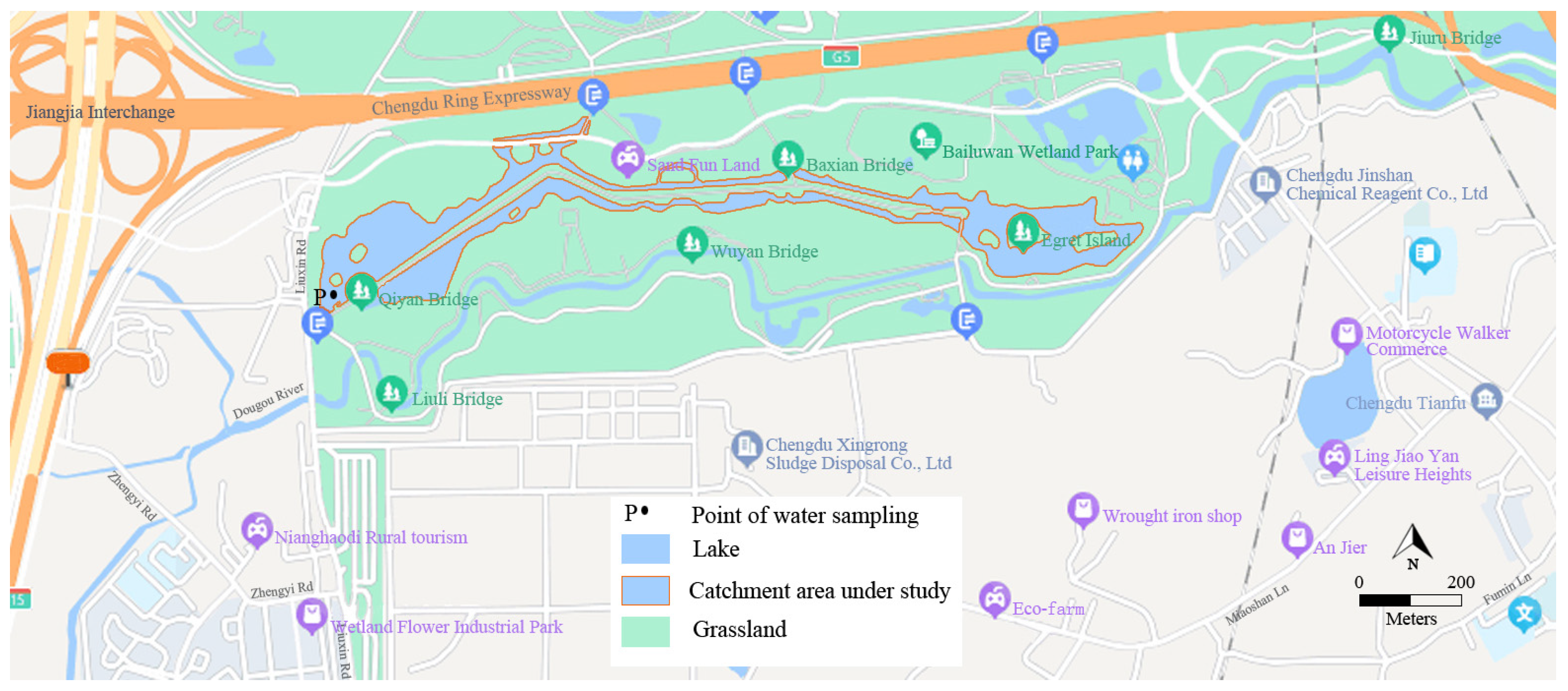
The research was carried out at Bailuwan Lake, with coordinates of 104°7′40.5″ E longitude and 30°34′56.01″ N latitude; this lake is situated within the round-the-city ecological zone, Chengdu, Sichuan, Southwest China (refer to Figure 1). It serves as an urban tourism eco-wetland, meticulously developed by the Jinjiang District Government. In 2017, it received recognition as the first National Urban Wetland Park in Chengdu, China. With a total area of 200 hectares, the lake encompasses approximately 67 hectares of open water surface and has depths ranging from 0.5 to 6.5 m. This lake is fed primarily by a tributary of the Dongfeng Canal (Dougou River), which discharges lake water to the outside through evaporation and ditches.
The study area has a humid subtropical climate with a mean annual temperature of 16.5 °C, with the lowest temperatures occurring in January and the highest in July or August. Throughout our 9-month investigation, the daily average air temperature surrounding the lake ranged between −5 and 30 °C (refer to Figure S1A), while the average annual precipitation was ca. 900 mm. On average, the annual solar radiation hours were approximately 1032, with higher radiation hours from April to August during the study period (see Figure S1B).
2.2. Field Measurements
During the study period, we conducted biweekly field visits from January to September 2020 to gather measurements of pCO2 and other relevant water quality parameters. However, due to the severe effects attributed to the new coronavirus COVID-19, we were not able to perform testing in February and March. To ensure accuracy and consistency, we selected a fixed location near the lake outlet for water sample collection and monitoring, as indicated in Figure 1. Throughout each field trip, we conducted in-situ measurements at 7:00, 10:00, 14:00, and 17:00 China Standard Time (CST) at about 2 m from the lake shore. All parameters were measured at 30–50 cm below the water surface, including pH, water temperature (twater), transparency (TPC), turbidity (FNU), electrical conductivity (EC), total dissolved solids (TDS), DO, bicarbonate (HCO3−; BCB), and carbonate (CO32−; CB). To reduce the influence of rainfall and runoff, we deliberately scheduled the field trips on sunny days, adjusting the timing accordingly. By monitoring the obtained pH, BCB and the Henry’s law constant (Kh) and ion concentrations in water, pCO2 in the carbonate system can be calculated [36]. Therefore, the mass fraction of CB and BCB can be calculated by titration using phenolphthalein and methyl orange as indicators for field monitoring.
Among the parameters measured, the TPC was determined utilizing a 200 mm diameter black-and-white disc, while the FNU was monitored by a HACH-TSS portable turbidimeter (Danaher Corporation, Washington, DC, USA). We evaluated pH, EC, TDS, and twater employing a Hanna-HI9829 detector (Hanna Instruments, Padua, Italy), while DO was detected using a Hanna-HI98186 equipment (Hanna Instruments, Padua, Italy).
To determine the water samples, we referred to the current Chinese methodological book The Analytical Methods for Water and Wastewater Monitoring (The 4th Edition) and the methods in the latest Chinese national standard The National Standard for Food Safety Test Methods for Drinking Natural Mineral Water [GB 8538-2022; The National Standard of the People’s Republic of China (published in Chinese); Issued 30 June 2022, and implemented 30 December 2022]. In brief, four drops of phenolphthalein indicator were added after transferring the collected 100 mL water sample to a 250 mL flask, and the solution turned red. Then, we titrated with a standard solution of hydrochloric acid until the color became clear. We recorded the volume of standard hydrochloric acid solution used for titration (called P). If the solution remained colorless with the addition of phenolphthalein indicator, we titrated with standard hydrochloric acid solution after adding three drops of methyl orange indicator in a conical flask until the solution changed from orange to orange-red. The volume (M) of the standard hydrochloric acid solution used for titration was recorded. We then determined the total volume of hydrochloric acid standard solution (T) consumed by the water sample according to Equation (1):
T = M + P
Considering different values of P (i.e., P = T, P > 1/2T, P = 1/2T, P < 1/2T, P = 0), the following Equations (2) and (3) were employed to determine the CB and BCB:
where CHA denotes the level of the HCl standard solution, while V indicates the volume of the measured water sample. In this study, CHA was 0.025 mol L−1, and V was 100 mL. Furthermore, the notation [30.005] represents the mass of CO32−, while [61.017] indicates the corresponding mass of HCO3− under the same conditions.
CB = [2 × P × CHA × 30.005]/V × 1000
BCB = [(M − P) × CHA × 61.017]/V × 1000
Once the field data collection was completed, we collected water samples for laboratory analysis at four specific time points during each trip: 7:00, 10:00, 14:00, and 17:00 CST. The water samples were collected using a customized polyethylene grab sampler that was specifically designed for this study. In brief, 500 mL of the collected lake water was added to 0.5 mL of MgCO3 suspension (1%) to determine the level of chlorophyll a (Chla) in the water [37]. The 3 mL of sulfuric acid was used for nitrate (NT; see Method S1) and total phosphorus (TP; Method S2) determination, while the filtered water sample (20 mL) was inspected for total carbon (TC), inorganic carbon (IC) and total dissolved nitrogen (TDN; Method S3). In addition, the filtered water samples (50 mL) were tested for four anions (fluoride/F−, chloride/Cl−, sulfate/SO42−, and nitrate/NO3−). To ensure proper preservation, all collected samples were stored in acid-washed high-density brown polyethylene bottles in a cooler to maintain their integrity during transportation.
2.3. Laboratory Analyses
2.3.1. Determination of Anions
In accordance with the National Environmental Protection Standard of the People’s Republic of China [HJ 84-2016 (published in Chinese); Issued 26 July 2016, and implemented 1 October 2016), the IC-2800 ion chromatography (Sichuan Keshengxin Environmental Technology Company, Chengdu, China) was employed to determine the four anions (F−, R2 = 0.9996; Cl−, R2 = 0.9991; NO3−, R2 = 0.9998; SO42−, R2 = 0.9999).
2.3.2. Detection of Metabolized Carbon
In our study, TC and IC were analyzed employing a total organic carbon analyzer of the TOC-L CPH Basic System (Shimadzu Corporation, Kyoto, Japan), and standard curves were plotted (IC: R2 = 1.0000; TC: R2 = 1.0000). To determine the total organic carbon (TOC) concentration (mg L−1), the following Equation (4) was used:
TOC = TC − IC
2.3.3. Eutrophication Evaluation
Based on the Methods and Technical Regulations for Eutrophication Evaluation of Lakes (Reservoirs) (Zhuzhan Shengzi (2001) No. 090) issued by the China Environmental Monitoring Center, the comprehensive nutrient status index (TLI (∑)) was used in this study to evaluate the eutrophication degree of this water body following Formula (5) (see Method S4 for details).
2.3.4. Calculation of pCO2
When the aqueous solution is in balance, the levels of HCO3−, CO32−, H2CO3 and dissolved CO2, which make up inorganic carbon, are dependent on the pH, twater and ionic strength (ref. [18,36,38,39,40]). Therefore, we used the CB equilibrium model to evaluate pCO2 according to the pH, HCO3−, CO32−, Kh, and ions with the following Equation (6):
where α(H+) and α(HCO3−) represent the ionic activities of [H+] and [HCO3−], respectively:
where I represents the ionic strength. However, the concentrations of the three cations ([K+], [Na+] and [Mg2+]) were not detected (n.d.) in this study. Therefore, Equation (9) can be simplified to (10) (see Method S5 for details):
α (H+) = 10−[pH]
I = 0.5([K+] + 4[Ca2+] + [Na+] + 4[Mg2+] + [Cl−] + 4[SO42−] + [NO3−] + [HCO3−])
I = 0.5(4[Ca2+] + [Cl−] + 4[SO42−] + [NO3−] + [HCO3−])
2.3.5. Estimation of fCO2
Previous studies have established that CO2 diffusion at the water–air interface is affected by temperature, salinity, wind speed and the disparity in pCO2. Therefore, we employed the model (11) to estimate the water–air fCO2 (refs. [41,42]).
where fCO2 represents the flux of water–air CO2. KH and KT represent the solubility and gas exchange rate of CO2 at a specific temperature, respectively. Among them, the KH is influenced by temperature, salinity, and pressure (cf. ref. [43]):
fCO2 = KT KH [pCO2(water) − pCO2(air)]
In addition, the normalized Schmidt number 600 (K600) was converted to the gas exchange rate (KT) of CO2 using Equation (13) [44]:
where n represents the Schmidt number exponent. Specifically, n is 0.50 for wind speeds above 3.7 m s−1, while n is 0.75 for wind speeds below 3.7 m s−1 [45]. In this study, a Schmidt number of 0.67 was used under typical conditions, as supported by the findings of [38]. In addition, the formula (14) for K600 and related explanations have been shown in Method S6. The U10 is the normalized wind speed at a height of 10 m above the water surface at the time of sampling.
K600 = 2.07 + 0.215U101.7
In the whole study, we employed the IBM-SPSS Statistics 22 software for statistical analysis and the SigmaPlot 14.0 for making graphs. Moreover, Tukey’s test was performed at a significance level of 0.05.
3. Results
3.1. Changes in pCO2
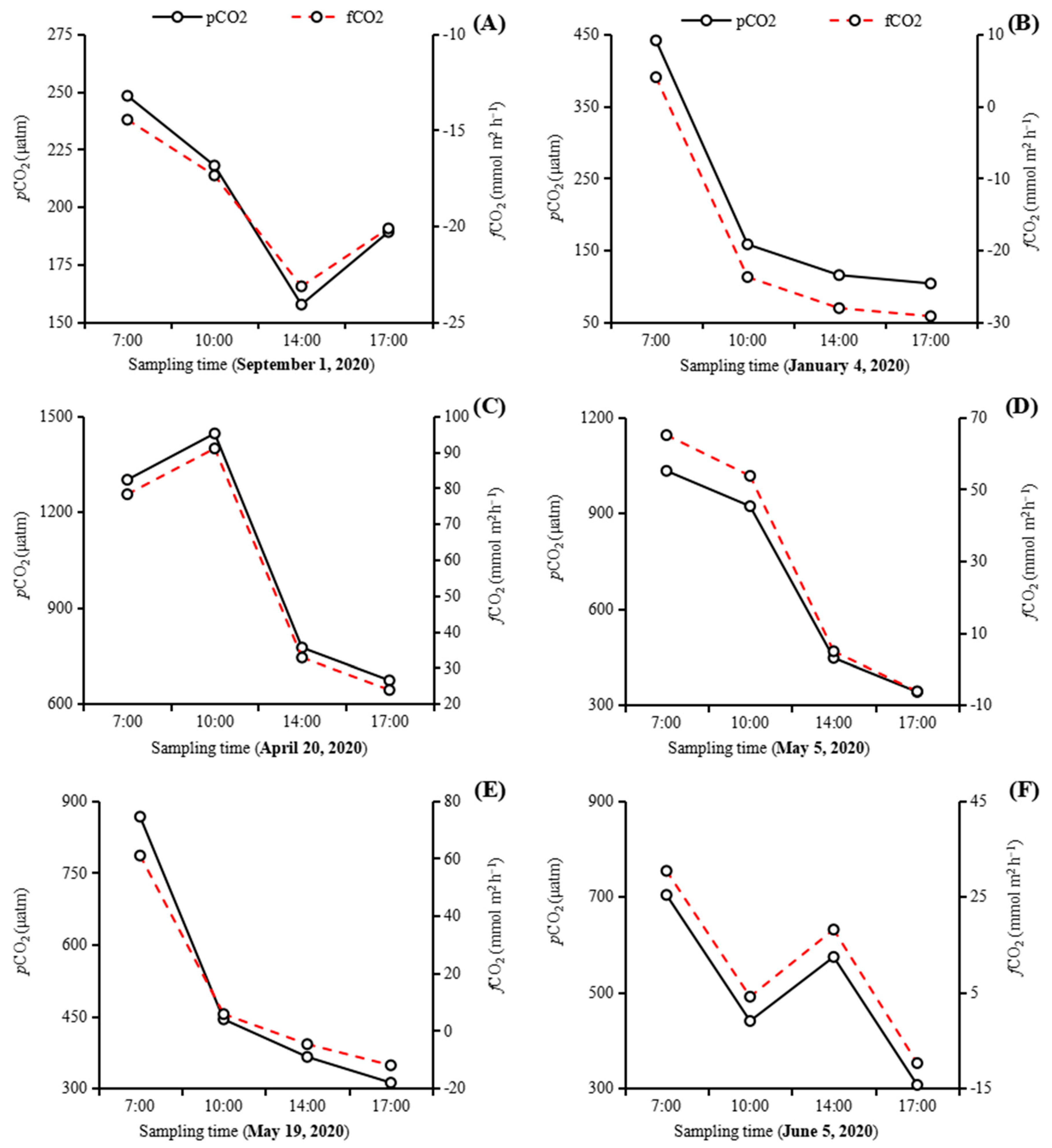
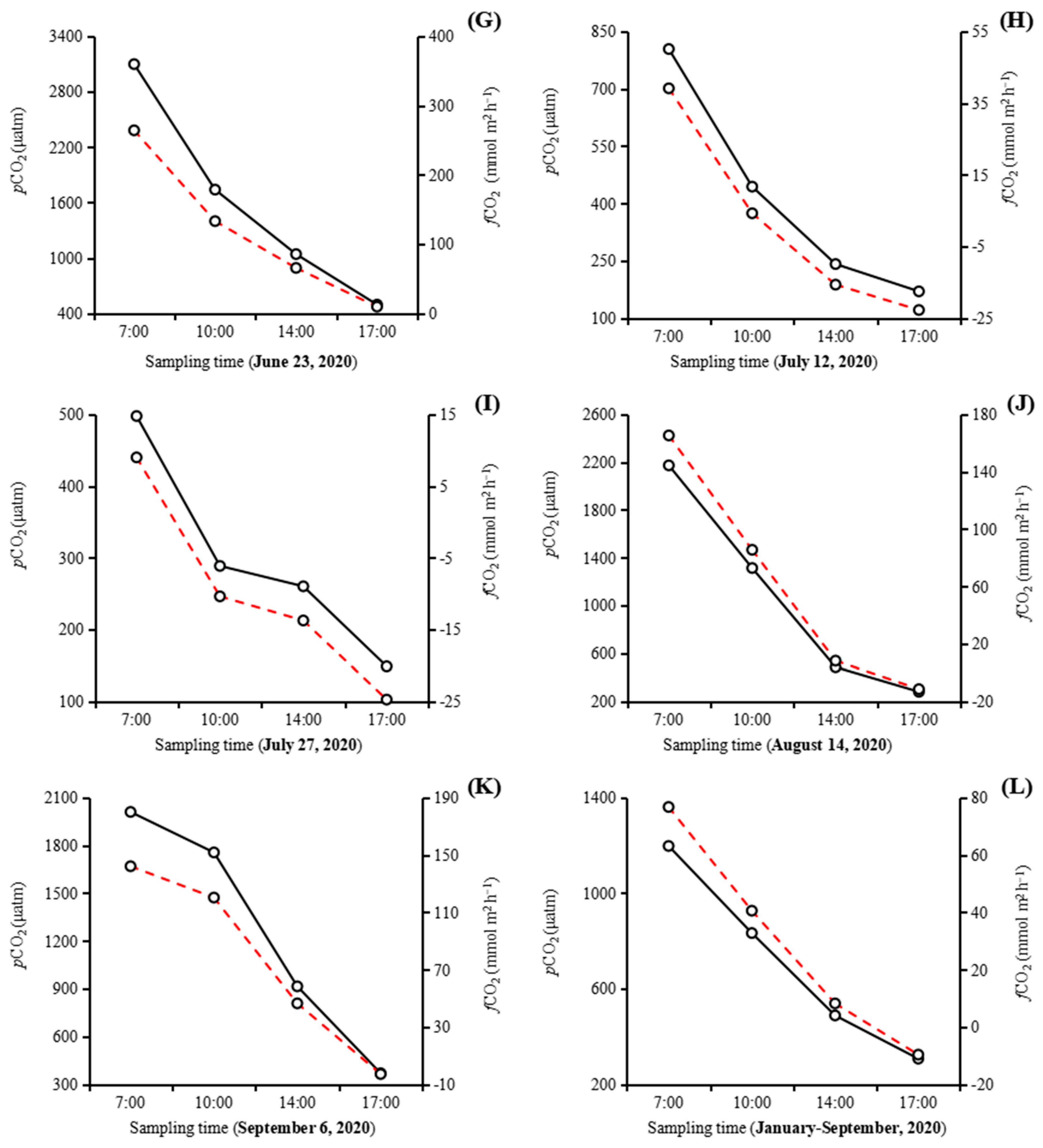
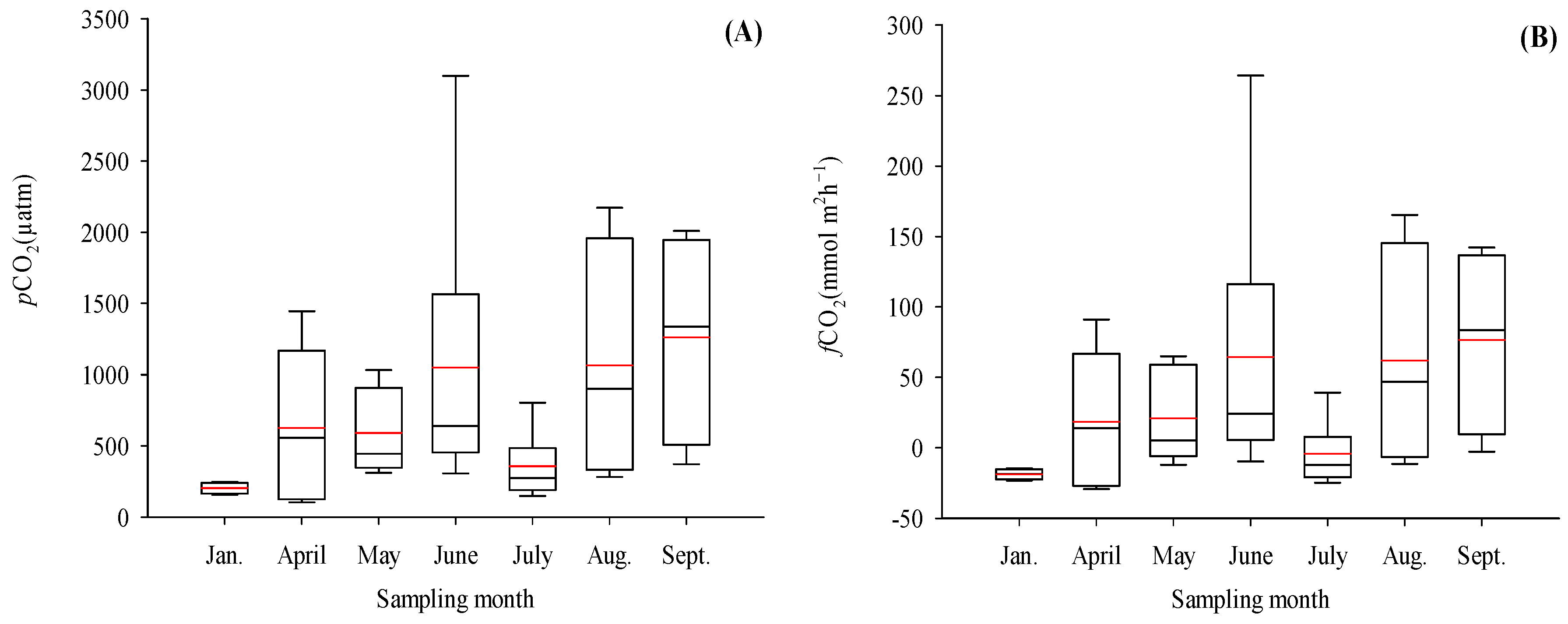
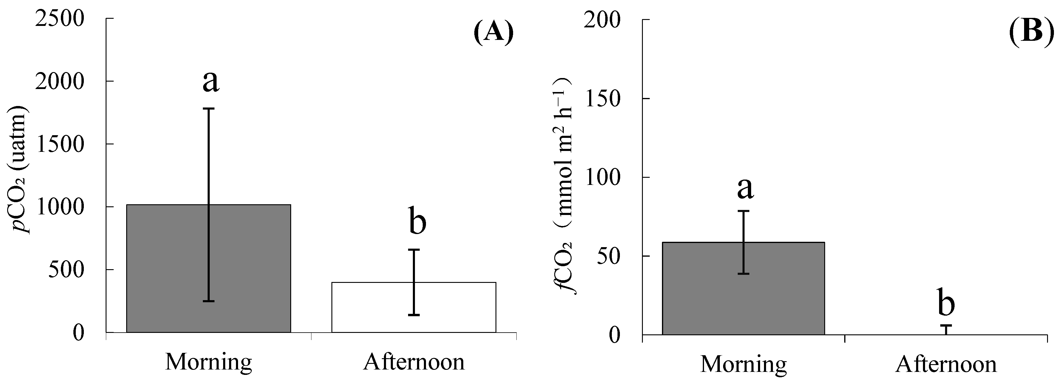
Our computational analysis revealed a clear continuous decreasing trend in pCO2 from early morning (7:00 CST) to afternoon (17:00 CST) for all 11 sampling days from January to September 2020 (Figure 2). The mean pCO2 decreased significantly (p < 0.05) from 10:00 to 17:00 (n = 11). The mean pCO2 decreased by ca. 29% from 7:00 (1198 ± 880 μatm) to 10:00 (834 ± 623 μatm), declined by ca. 50% from 10:00 to 14:00 (489 ± 309 μatm) and reduced by ca. 47% from 14:00 to 17:00 (308 ± 166 μatm). The average daytime pCO2 throughout our study (n = 44) was 707 ± 642 μatm. The highest daytime mean pCO2 was observed in September (1263 ± 756 μatm; n = 4), while the lowest occurred in January 2020 (203 ± 39 μatm; n = 4; Figure 3). Moreover, our analysis found a significant (p < 0.05) disparity in the pCO2 levels of the lake during the morning (7:00–12:00 CST) and afternoon (12:00–17:00 CST) periods. The average pCO2 values recorded were 1016 ± 767 μatm and 399 ± 259 μatm, respectively, based on a sample size of 22 (Figure 4A).
3.2. Variations in fCO2
Similar to the diurnal variation in pCO2, CO2 fluxes (fCO2) for all 11 of our sampling days also showed a decreasing trend during the day (Figure 2). All samples showed a significant (p < 0.05) decrease in diurnal fCO2 between 7:00 CST and 14:00 CST, except for 20 April 2020 (daytime fCO2 of 78 at 7:00 and 91 mmol m2 h−1 at 10:00). Regarding the whole investigation period, the mean fCO2 at 7:00 was significantly reduced by ca. 47% (41 ± 58 mmol m2 h−1) at 10:00 and ca. 89% (8 ± 330 mmol m2 h−1) at 14:00, respectively (n = 4), while the mean fCO2 at 17:00 decreased to ca. 112% (−10 ± 16 mmol m2 h−1). We also observed that the mean daytime fCO2 throughout the study period was lowest in January, when it was highest in September 2020, with an overall mean of 29 (± 67) mmol m2 h−1 (n = 11; Figure 3). Likewise, for pCO2, a marked discrepancy (p < 0.05) in fCO2 between morning (59 ± 72 mmol m2 h−1) and afternoon (−1 ± 25 mmol m2 h−1) was also recorded (n = 22; Figure 4B).
3.3. Ambient Factors of CO2
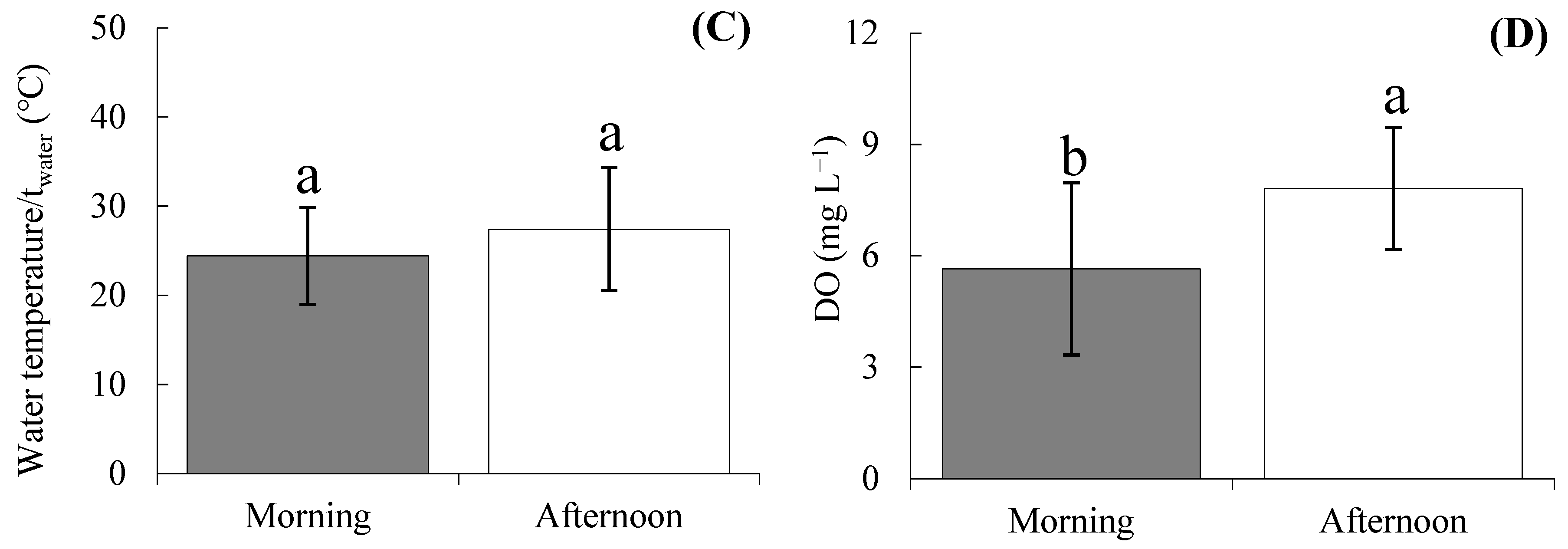
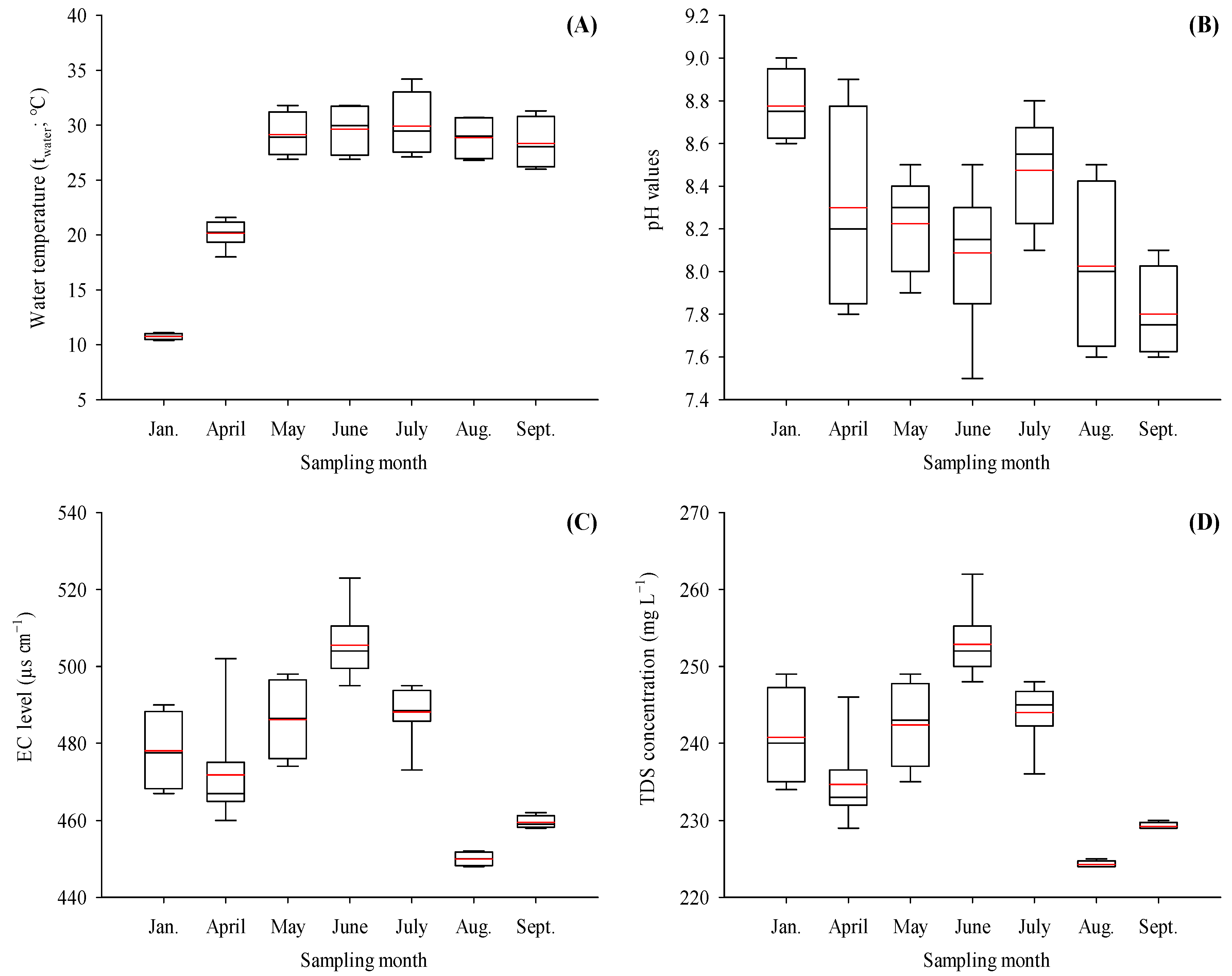
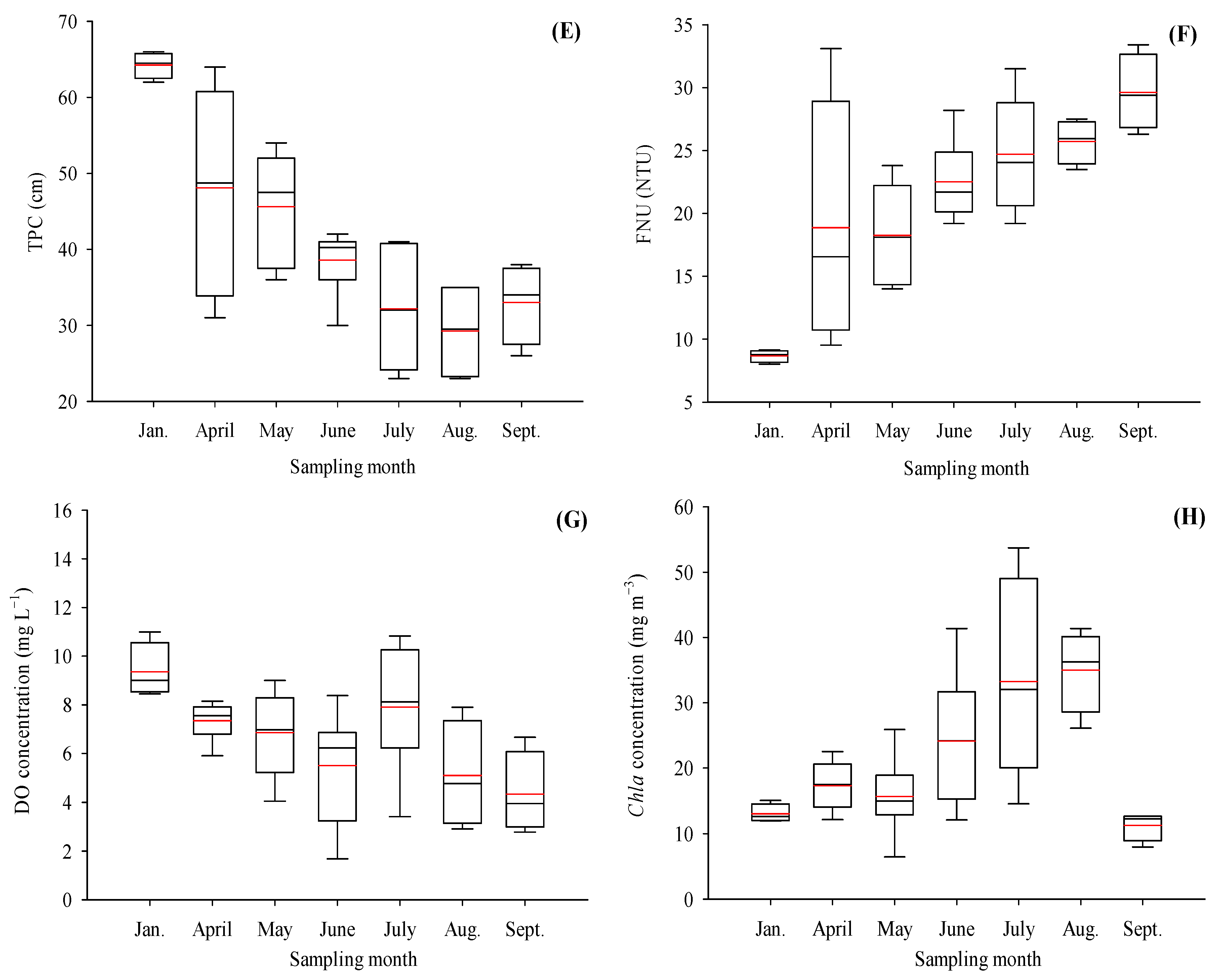
In this studied lake, the mean DO of the water–air interface in the morning was significantly (p < 0.05) lower than that in the afternoon (n = 22), while the mean water temperature (twater) had no marked difference (p > 0.05) between the morning and the afternoon. For other parameter changes, the twater, EC, TDS, TPC and FNU during the daytime exhibited no significant discrepancy at the four times, while pH, DO and Chla all reached their highest values at 17:00, with 8.48 ± 0.25, 8.60 ± 1.41 mg L−1 and 22.96 ± 15.63 mg m−3, respectively (Table 1).
To accurately reflect the nutrient status of the water bodies in Bailuwan Lake, we also calculated the TLI(∑) based on Equation (5) (Method S4). Our analysis showed that the four parameters (NT, TDN, TP and Chla; Table 1 and Figure S2) used to calculate TLI(∑) were apparently different at four different sampling times. The calculated TLI(∑) was 63.52 (60 < TLI(∑) ≤ 70; Table 2 and Table S1), indicating that Bailuwan Lake is middle-eutrophic. Furthermore, in accordance with the Surface Water Environmental Quality Standard of China [GB 3838-2002; The National Standard of the People’s Republic of China (published in Chinese); Issued 28 April 2002, and implemented 1 June 2002], we conducted tests to assess the levels of the four anions in water. Our results indicated that the water quality of Bailuwan Lake met the criteria for class I classification, as shown in Table S2.
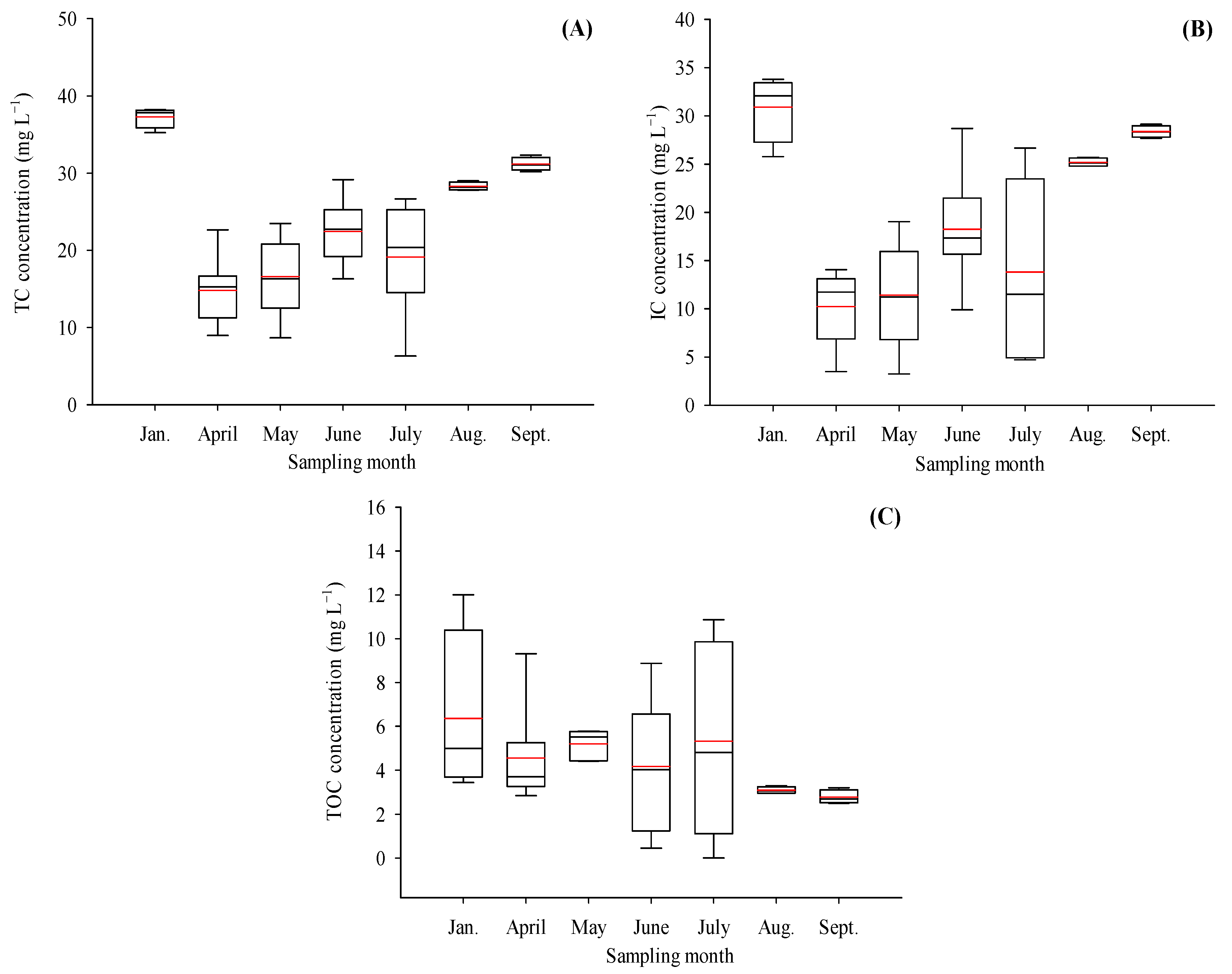
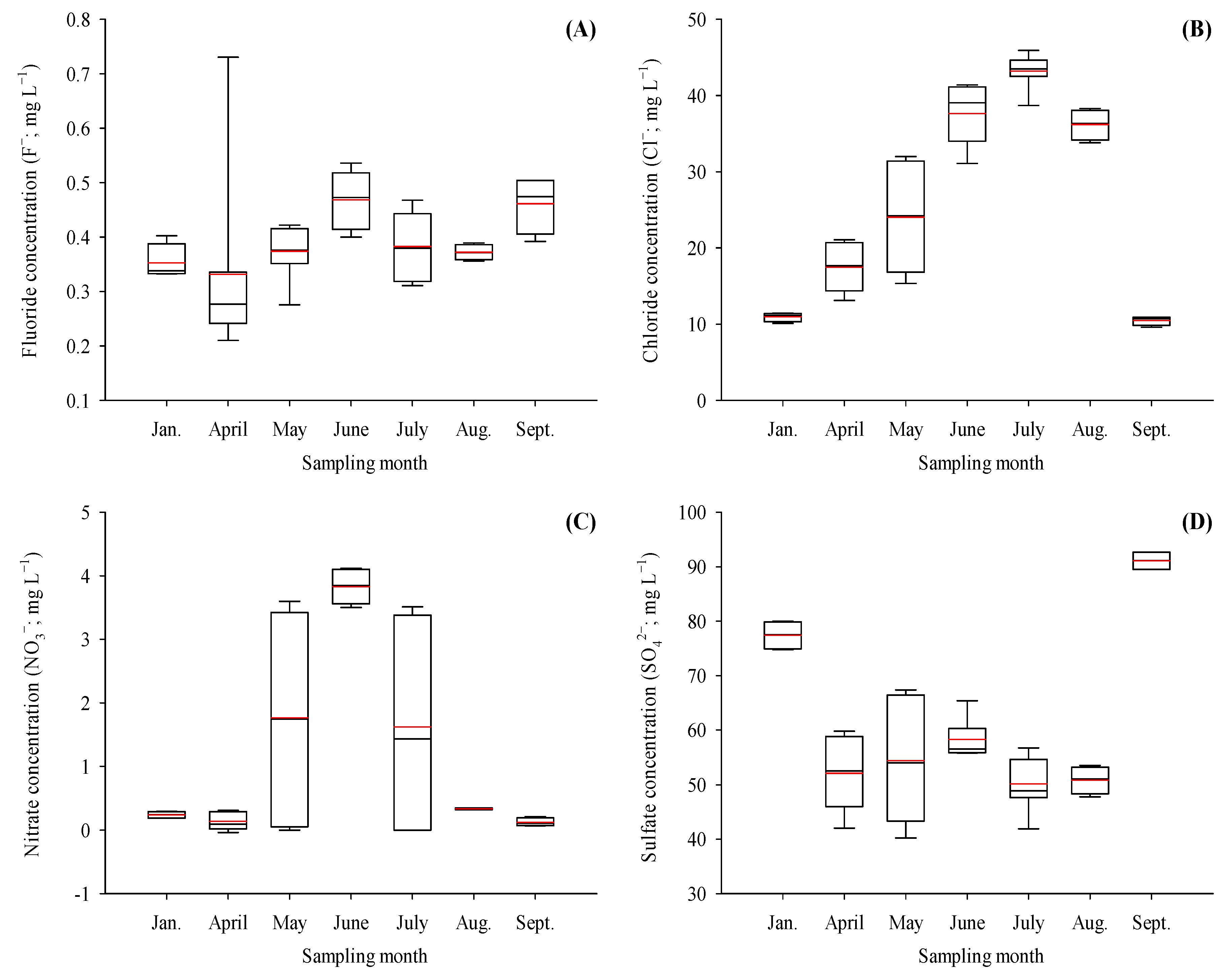
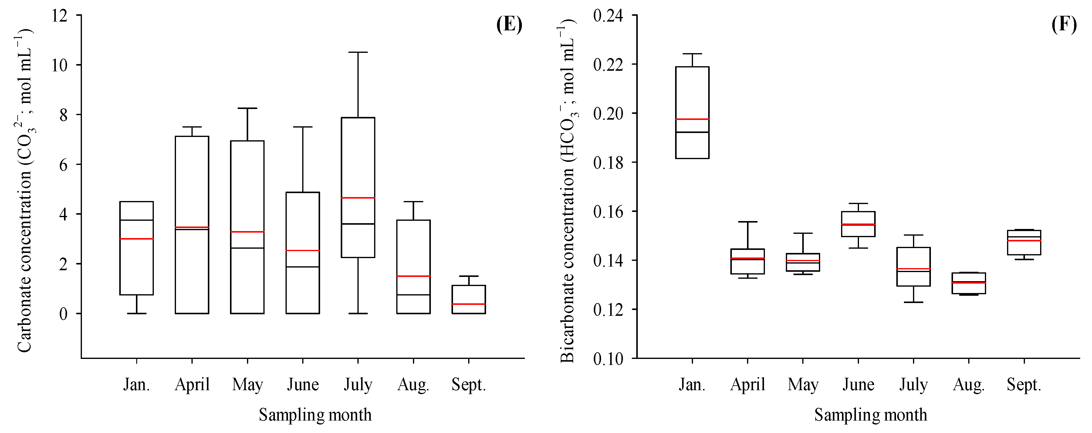
For the monthly variation, all water environment parameters showed significant differences across investigation months (Figure 5, Figure 6 and Figure 7). Interestingly, as twater gradually increased to stabilization (p > 0.05) from January to September, DO and TPC decreased significantly, while FNU increased gradually, but Chla and chloride decreased sharply in September 2020 (Figure 5 and Figure 7). In addition, the water bicarbonate concentration (Figure 7F) was highest in January, while it was markedly lower and stable (p > 0.05) in other months, and the water TC and IC decreased from April and then gradually increased until September 2020 (Figure 6A,B).
4. Discussion
By the end of 2019, more than 60% of China’s resident population had become urbanized [46,47]. The process of urbanization has been rapidly advancing, accompanied by human activities that have inevitably impacted inland freshwater systems, including urban lakes, affecting their water-carbon cycling [3,27,48]. Therefore, it is crucial to investigate the dynamics of carbon sink/source behaviors in lakes, along with their influencing factors. It is crucial to understand the carbon balance of urban lakes in developing countries, which could help promote carbon neutrality and peak carbon emissions.
4.1. Changes in the pCO2 Contribution to the Source–Sink Interchange
In this study, there was a significant overall decrease in pCO2 and fCO2 from January to September 2020 (n = 11) between 7:00 CST and 17:00 CST (Figure 2). Moreover, the average pCO2 during the mornings (7:00–12:00 CST; n = 22) was markedly (p > 0.05) higher than that in the afternoons (12:00–17:00 CST; Figure 3) in this middle-eutrophic lake, indicating that the dynamics of pCO2 in this system are mainly driven by biological photosynthesis (P) [10,49], influenced by the balance between P and respiration (R) [19,50]. Our previous work [10,20,24] and other studies in aquatic systems [21,33] have also obtained similar findings. In general, both P and R abide by the circadian rhythms, i.e., C fixation occurs only during the day, whereas respiration occurs throughout the 24 h cycle [27,51]. In our study, a significant negative correlation between DO and pCO2/fCO2 was observed (i.e., pCO2/DO = −0.801**, fCO2/DO= −0.811**) (Table 3 and Table S3), indicating that surface pCO2 is primarily driven by respiration and exceeds atmospheric CO2 levels when P is less than R (i.e., heterotrophic). Conversely, in autotrophic ecosystems, pCO2 was lower than atmospheric CO2 [20,35]. When P:R > 1.0, lakes may experience CO2 over-saturation. Previous studies have shown that inorganic carbon storage has a strong influence on dissolved CO2 concentrations in selected lakes and reservoirs in the United States [6,27,52].
Moreover, the average daytime pCO2 was 707 ± 642 μatm (n = 44), which was significantly elevated compared to typical atmospheric CO2 levels (i.e., 380–420 μatm; [17,18,53]). This observation indicated that the biological productivity at a depth of 1.0 m exceeded the dissolution of water CO2, with the potential for CO2 to be released into the atmosphere [10,54]. Thus, to some extent, it can be considered that this lake becomes a ‘source’ of CO2 during the day. Interestingly, the average pCO2 on 9th January, 1st April, and 27th July 2020 was lower than typical atmospheric CO2 levels (n = 4), with values of 203 ± 39 μatm, 205 ± 106 μatm, and 299 ± 146 μatm, respectively (Table 3). Similar phenomena were also observed in our studies on Capitol Lake, University Lake and Qinglonghu Lake [10,20,24]. One possible reason is the influence of increased precipitation on the sampling days (Figure 1). In terms of diurnal variation, a higher cumulative precipitation can lead to a significant increase in daily pCO2 variations, thus promoting CO2 exchange [55]. Additionally, owing to the relative openness of the sampling sites, higher wind speeds accelerated the exchange of soluble gases with the atmosphere, resulting in a decrease in pCO2. Consistent with previous studies, the regression between pCO2 and wind speed had a significant negative correlation with no time lag [56], suggesting that accelerated gas exchange between CO2 and water is the main process driving the decline in pCO2 [57,58]. Based on these findings, this urbanizing lake has the potential to function as both ‘source’ and ‘sink’ of CO2 during daytime hours.
4.2. Environmental Factors Affecting the Lake pCO2 and fCO2
In the present publications, the variations regarding pCO2 and fCO2 in lakes were closely related to environmental factors such as nutrient status, DO, pH and TPC/FNU. We focused on a lake in the central urban area of Chengdu, China, that is inevitably influenced by residential and industrial areas, despite being classified as a middle-eutrophic lake. This study revealed that high nutrient content could significantly stimulate the biological activity of aquatic phosphorus and thus increase CO2 uptake. Further, the enrichment of nutrients enhanced the decomposition of organic matter by fostering the proliferation of aquatic organisms, leading to an augmented release of CO2 [10,20,42]. This finding aligns with the significant negative correlation (R2 = −0.801**) observed between DO and pCO2 in this study. For instance, the dynamic fluctuations in CO2 in typical highly productive tropical lakes depend heavily on the diurnal biological metabolism cycle [59], whereas no significant diurnal variation in fCO2 has been observed in low-nutrient lakes [60].
DO plays an important role in maintaining the respiration and metabolic processes of organisms in water, which is affected by multiple factors such as twater, pressure, flow rate, and organic matter in water. Among them, twater is crucial in influencing the concentration of DO. Under the same water pressure and water velocity conditions, a lower water temperature correlates to a higher concentration of dissolved oxygen in water. In our study, the water temperature gradually increased from January to September, while the DO gradually decreased from January to September. As shown in Table 1 and Table S3, the water temperature was negatively correlated with DO (R2 = −0.189) because the oxygen molecules were more easily dissolved in water at low temperatures.
The continuous dissolution of atmospheric CO2 also could drive changes in lake water pH, altering the response of aquatic species to pH-sensitive pollutants [7,61]. In agreement with the results obtained in this investigation, a notable inverse relationship between pCO2/fCO2 and pH (Table S3) was observed, indicating a critical pH threshold where a shift occurred from CO2 absorption capacity to emission sources. In river wetlands, a pH exceeding 8.59 indicates a CO2 sink, while a pH below 8.59 acts as a carbon source [18,30]. Hence, we hypothesize that dramatic changes in pH and nutrient levels in lake systems are closely linked to urbanization, leading to elevated pCO2 levels in the water body [7,62].
Lake depth is also a factor to consider when estimating CO2 flux. Generally, the dynamics of CO2 in deep lakes are more complex than those in shallow lakes due to variations in sunlight availability and gas transfer between layers [63]. In this study, TPC and pCO2 at a sampling depth of 1 m showed a significant negative correlation, while FNU exhibited an obvious positive correlation (p < 0.05; Table S3). Similar results have been found in other aquatic systems. For instance, Podgrajsek et al. [58] reported higher nighttime CO2 flux levels than daytime levels in a shallow 1.3 m lake in central-eastern Sweden, which could be attributed to water-edge convection. In deep lakes, primary production often occurs in the upper water column, while R may prevail in the oxygen-depleted deep layers. This conclusion was validated by Liu et al. [64] in the deep (4–8 m) Ross Barnett Reservoir in Mississippi, USA. Furthermore, Spafford and Risk [63] investigated a deep (>20 m) oligotrophic lake in Canada and found distinct diurnal peaks of CO2 evaporation between 1:00 and 10:00 Atlantic Daylight Time (ADT). The CO2 net exchange rates decreased during daylight hours until the minimum solar radiation (ADT 17:00–21:00). This diurnal exchange pattern, similar to shallow lakes, may be influenced by microstratification and lateral variations in substrate composition and carbon.
4.3. Uncertainties in the Current Estimates of the Lake CO2 Escape
In recent years, many studies have focused on quantifying CO2 escapes from freshwater to the atmosphere. [3,65,66]. However, different studies have shown substantial variations in global estimates of CO2 release from inland freshwater systems such as lakes and reservoirs (0.06–0.84 Pg C year−1; e.g., [1,2,15,38,50,67]). The potential reasons for these large discrepancies include geographical differences [51,59,68,69], limitations of methods [15,70,71], and temporal variability [65,72,73]. Notably, current estimates of fCO2 often suffer from poor coverage of low-frequency time series, such as monthly or seasonal sampling data. In our study, the rapid decline in daytime water–air pCO2/fCO2 occurred within a very short time frame, suggesting that one-time measurements commonly used in previous studies may tend to underestimate or overestimate daily CO2 outgassing. On the other hand, the observations in this study were conducted from 7:00 to 17:00, without nighttime measurements. Nighttime CO2 outgassing is often more pronounced when dark P is nearly inactive, possibly due to favorable conditions for respiration (P:R < 1.0) or intense physical changes in lake water [33]. Gu et al. [35] conducted an analysis of lake data collected between 1987 and 2006 and discovered a slight increase in average nighttime pCO2 (224 µatm) compared to daytime levels. Similarly, Reis and Barbosa [59] examined a tropical lake (P-type) in Brazil and observed that the mean nighttime pCO2 (from 21:00 to 17:00 BRT) was higher than the daytime pCO2 (from 9:00 to 17:00 BRT, approximately 436 m). Moreover, measurements directly recorded from the Ross Barnett Reservoir indicated that nighttime fCO2 was approximately 70% higher than daytime levels (8:00–20:00 CST) during a one-year observational period [64]. Based on these findings, we therefore believe that current estimates of CO2 evaporation from lakes, at regional or global scales, may be significantly underestimated. To standardize and reduce uncertainties in CO2 evaporation estimates, it is crucial to understand and constrain all factors that may contribute to data dispersion and differences and to further enhance monitoring at smaller timescales, particularly during the nighttime.
5. Conclusions
In this work, for the daily variability, a significant and continuous decrease in average pCO2 and fCO2 from early morning to evening was observed. Specifically, on the one hand, the average pCO2 decreased by ca. 29% from 7:00 to 10:00, by ca. 50% from 10:00 to 14:00, and by ca. 47% from 14:00 to 17:00. Compared to 7:00, the average fCO2 significantly decreased by ca. 112% at 17:00. Throughout the study period, the average daytime pCO2 and fCO2 were 707 ± 642 μatm (higher than typical atmospheric CO2 levels of 380–420 μatm) and 29 ± 67 mmol m2 h−1, respectively, although the average pCO2 on 9 January, 1 April, and 27 July was lower than typical atmospheric CO2 levels. The pCO2 and fCO2 were significantly higher in the mornings than in the afternoons (p < 0.05). Each month, all water environment parameters showed significant differences. These above findings suggest that this studied urbanizing lake has the potential to act as both a ‘source’ and ‘sink’ of CO2 during the daytime. However, there are significant discrepancies in global estimates of CO2 emissions from inland freshwater systems, which could be attributed to geographical differences, methodological limitations, and temporal variations. To reduce uncertainties in CO2 evaporation estimates, it is crucial to further constrain all factors that may contribute to data dispersion and differences, especially by enhancing monitoring at smaller timescales, such as during nighttime.
Supplementary Materials
The following supporting information can be downloaded at: https://www.mdpi.com/article/10.3390/w15193365/s1, Method S1: Determination of NT. Method S2: Determination of TP. Method S3: Determination of TDN. Method S4 Eutrophication evaluation. Method S5: Calculation of pCO2. Method S6: Estimation of CO2 fluxes. Figure S1: Daily air temperature and precipitation (A; mm d−1) and radiation (B; h d−1) during the study period in Bailuwan Lake. Figure S2: Monthly and hourly changes of water NT (A, B), TDN (C, D) and TP (E, F) in Bailuwan Lake. Table S1: Correlation between parameters of Chinese lakes/reservoirs and Chla with rij and rij2. Table S2: Concentrations and evaluation of water anion levels in Bailuwan Lake. Table S3: Pearson correlation analysis of environmental parameters in Bailuwan Lake (n = 44) at p < 0.05. References [10,20,24,37,38,41,43,44,45,73] are cited in the supplementary materials.
Author Contributions
R.Y.: Conceptualization, Methodology, Formal analysis, Investigation, Data Curation, Writing—Original Draft, Funding acquisition. Y.C.: Software, Formal analysis, Investigation. D.L.: Investigation. Y.Q.: Investigation. K.L.: Investigation. S.L.: Conceptualization, Methodology, Data Curation, Writing—Review and Editing, Funding acquisition. H.S.: Writing-Review and Editing, Supervision, Project administration, Funding acquisition. All authors have read and agreed to the published version of the manuscript.
Funding
This work was partially supported by the Sponsored Project of Sichuan Landscape and Recreation Research Center (No. JGYQ2023003), and the Leadership Talent Program of the Tianfu Emei Plan in Sichuan Province (No. CHUANEMEI2105).
Data Availability Statement
Not applicable.
Acknowledgments
The authors are thankful to Sichuan Keshengxin Environmental Technology Co., Ltd., and College of Environmental Sciences at Sichuan Agricultural University. Special thanks are extended to Li Li, Ting Lei, Lijuan Yang, Zan Zou, Jia Wei, Qianrui Liu, Xiaoyang Ke, Xingyu Zhu, Jianglin Yu, Hongyu Wu and other research assistants. The authors express their gratitude to the Bailuwan Lake Management Center for granting permission and providing transportation.
Conflicts of Interest
The authors declare no conflict of interest.
References
- Liang, J.; Tang, W.; Zhu, Z.; Li, S.; Wang, K.; Gao, X.; Li, X.; Tang, N.; Lu, L.; Li, X. Spatiotemporal variability and controlling factors of indirect N2O emission in a typical complex watershed. Water Res. 2023, 229, 119515. [Google Scholar] [CrossRef]
- Zhu, Z.; Li, X.; Bu, Q.; Yan, Q.; Wen, L.; Chen, X.; Li, X.; Yan, M.; Jiang, L.; Chen, G.; et al. Land–water transport and sources of nitrogen pollution affecting the structure and function of riverine microbial communities. Environ. Sci. Technol. 2023, 57, 2726–2738. [Google Scholar] [CrossRef]
- Sun, H.; Yu, R.; Liu, X.; Cao, Z.; Li, X.; Zhang, Z.; Wang, J.; Zhuang, S.; Ge, Z.; Zhang, L.; et al. Drivers of spatial and seasonal variations of CO2 and CH4 fluxes at the sediment water interface in a shallow eutrophic lake. Water Res. 2022, 222, 118916. [Google Scholar] [CrossRef]
- Chen, S.; Hu, C.; Cai, W.; Yang, B. Estimating surface pCO2 in the northern Gulf of Mexico: Which remote sensing model to use? Cont. Shelf Res. 2017, 151, 94–110. [Google Scholar] [CrossRef]
- Chen, S.; Hu, C. Environmental controls of surface water pCO2 in different coastal environments: Observations from marine buoys. Cont. Shelf Res. 2019, 183, 73–86. [Google Scholar] [CrossRef]
- Li, X.; Shi, F.; Ma, Y.; Zhao, S.; Wei, J. Significant winter CO2 uptake by saline lakes on the Qinghai-Tibet Plateau. Glob. Change Biol. 2022, 28, 2041–2052. [Google Scholar] [CrossRef]
- Minor, E.C.; Brinkley, G. Alkalinity, pH, and pCO2 in the Laurentian Great Lakes: An initial view of seasonal and inter-annual trends. J. Great Lakes Res. 2022, 48, 502–511. [Google Scholar] [CrossRef]
- Pachauri, R.K.; Allen, M.R.; Barros, V.R.; Broome, J.; Cramer, W.; Christ, R.; Church, J.A.; Clarke, L.; Dahe, Q.; Dasgupta, P.; et al. Climate change 2014: Synthesis report. Contribution of Working Groups I, II and III to the Fifth Assessment Report of the Intergovernmental Panel on Climate Change; Intergovernmental Panel on Climate Change (IPCC): Geneva, Switzerland, 2014. [Google Scholar]
- Wen, Z.; Song, K.; Shang, Y.; Fang, C.; Li, L.; Lv, L.; Lv, X.; Chen, L. Carbon dioxide emissions from lakes and reservoirs of China: A regional estimate based on the calculated pCO2. Atmos. Environ. 2017, 170, 71–81. [Google Scholar] [CrossRef]
- Yang, R.; Xu, Z.; Liu, S.; Xu, Y.J. Daily pCO2 and CO2 flux variations in a subtropical mesotrophic shallow lake. Water Res. 2019, 153, 29–38. [Google Scholar] [CrossRef]
- Marce, R.; Obrador, B.; Morgui, J.A.; Riera, J.L.; Lopez, P.; Armengol, J. Carbonate weathering as a driver of CO2 supersaturation in lakes. Nat. Geosci. 2015, 8, 107–111. [Google Scholar] [CrossRef]
- Li, S.; Luo, J.; Xu, X.J.; Zhang, L.; Ye, C. Hydrological seasonality and nutrient stoichiometry control dissolved organic matter characterization in a headwater stream. Sci. Total Environ. 2022, 807, 150843. [Google Scholar] [CrossRef]
- Zhang, L.; Xu, Y.J.; Li, S. Source and quality of dissolved organic matter in streams are reflective to land use/land cover, climate seasonality and pCO2. Environ. Res. 2023, 216, 114608. [Google Scholar] [CrossRef]
- Cole, J.J.; Caraco, N.F.; Kling, G.W.; Kratz, T.K. Carbon dioxide supersaturation in the surface waters of lakes. Science 1994, 265, 1568–1570. [Google Scholar] [CrossRef]
- Raymond, P.A.; Hartmann, J.; Lauerwald, R.; Sobek, S.; McDonald, C.; Hoover, M.; Butman, D.; Striegl, R.; Mayorga, E.; Humborg, C.; et al. Global carbon dioxide emissions from inland waters. Nature 2013, 503, 355–359. [Google Scholar] [CrossRef]
- Keller, P.S.; Catalán, N.; von Schiller, D.; Grossart, H.P.; Koschorreck, M.; Obrador, B.; Frassl, M.A.; Karakaya, N.; Barros, N.; Howitt, J.A.; et al. Global CO2 emissions from dry inland waters share common drivers across ecosystems. Nat. Commun. 2020, 11, 2126. [Google Scholar] [CrossRef]
- Abril, G.; Martinez, J.M.; Artigas, L.F.; Moreira-Turcq, P.; Benedetti, M.F.; Vidal, L.; Meziane, T.; Kim, J.H.; Bernardes, M.C.; Savoye, N.; et al. Amazon River carbon dioxide outgassing fuelled by wetlands. Nature 2014, 505, 395–398. [Google Scholar] [CrossRef]
- Li, Q.; Guo, X.; Zhai, W.; Xu, Y.; Dai, M. Partial pressure of CO2 and air-sea CO2 fluxes in the South China Sea: Synthesis of an 18-year dataset. Prog. Oceanogr. 2020, 182, 102272. [Google Scholar] [CrossRef]
- Karim, A.; Dubois, K.; Veize, J. Carbon and oxygen dynamics in the Laurentian Great Lakes: Implications for the CO2 flux from terrestrial aquatic systems to the atmosphere. Chem. Geol. 2011, 281, 133–141. [Google Scholar] [CrossRef]
- Yang, R.; Chen, Y.; Du, J.; Pei, X.; Li, J.; Zou, Z.; Song, H. Daily Variations in pCO2 and fCO2 in a Subtropical Urbanizing Lake. Front. Earth Sci. 2022, 9, 805276. [Google Scholar] [CrossRef]
- Tonetta, D.; Fontes, M.L.S.; Petrucio, M.M. Determining the high variability of pCO2 and pO2 in the littoral zone of a subtropical coastal lake. Acta Limnol. Bras. 2014, 26, 288–295. [Google Scholar] [CrossRef]
- Couturier, M.; Prairie, Y.T.; Paterson, A.M.; Emilson, E.J.S.; del Giorgio, P.A. Long-Term Trends in pCO2 in Lake Surface Water Following Rebrowning. Geophys. Res. Lett. 2022, 49, e2022GL097973. [Google Scholar] [CrossRef]
- Marotta, H.; Duarte, C.M.; Meirelles-Pereira, F.; Bento, L.; Esteves, F.A.; Enrich-Prast, A. Long-term CO2 variability in two shallow tropical lakes experiencing episodic eutrophication and acidification events. Ecosystems 2010, 13, 382–392. [Google Scholar] [CrossRef]
- Xu, Y.J.; Xu, Z.; Yang, R. Rapid daily change in surface water pCO2 and CO2 evasion: A case study in a subtropical eutrophic lake in Southern USA. J. Hydrol. 2019, 570, 486–494. [Google Scholar] [CrossRef]
- Marotta, H.; Duarte, C.M.; Sobek, S.; Enrich-Prast, A. Large CO2 disequilibria in tropical lakes. Glob. Biogeochem. Cycles 2009, 23, GB4022. [Google Scholar] [CrossRef]
- Kosten, S.; Roland, F.; Marques, D.M.L.D.M.; Van Nes, E.H.; Mazzeo, N.; Sternberg, L.S.L.; Scheffer, M.; Cole, J.J. Climate-dependent CO2 emissions from lakes. Glob. Biogeochem. Cycles 2010, 24, GB2007. [Google Scholar] [CrossRef]
- Katkov, E.; Fussmann, G.F. The effect of increasing temperature and pCO2 on experimental pelagic freshwater communities. Limnol. Oceanogr. 2023, 68, S202–S216. [Google Scholar] [CrossRef]
- Sabine, C.L.; Feely, R.A.; Gruber, N.; Key, R.M.; Lee, K.; Bullister, J.L.; Wanninkhof, R.; Wong, C.S.; Wallace, D.W.R.; Tilbrook, B.; et al. The oceanic sink for anthropogenic CO2. Science 2004, 305, 367–371. [Google Scholar] [CrossRef]
- Yan, H.; Yu, K.; Shi, Q.; Lin, Z.; Zhao, M.; Tao, S.; Liu, G.; Zhang, H. Air-sea CO2 fluxes and spatial distribution of seawater pCO2 in Yongle Atoll, northern-central South China Sea. Cont. Shelf Res. 2018, 165, 71–77. [Google Scholar] [CrossRef]
- Jia, J.; Sun, K.; Lü, S.; Li, M.; Wang, Y.; Yu, G.; Gao, Y. Determining whether Qinghai–Tibet Plateau waterbodies have acted like carbon sinks or sources over the past 20 years. Sci. Bull. 2022, 67, 2345–2357. [Google Scholar] [CrossRef]
- Crawford, J.T.; Loken, L.C.; Stanley, E.H.; Stets, E.G.; Dornblaser, M.M.; Striegl, R.G. Basin scale controls on CO2 and CH4 emissions from the Upper Mississippi River. Geophys. Res. Lett. 2016, 43, 1973–1979. [Google Scholar] [CrossRef]
- Liu, S.; Lu, X.X.; Xia, X.; Yang, X.; Ran, L. Hydrological and geomorphological control on CO2 outgassing from low-gradient large rivers: An example of the Yangtze River system. J. Hydrol. 2017, 550, 26–41. [Google Scholar] [CrossRef]
- Wang, L.; Mei, W.; Yin, Q.; Guan, Y.; Le, Y.; Fu, X. The variability in CO2 fluxes at different time scales in natural and reclaimed wetlands in the Yangtze River estuary and their key influencing factors. Sci. Total Environ. 2021, 799, 149441. [Google Scholar] [CrossRef]
- Richey, J.E.; Melack, J.M.; Aufdenkampe, A.K.; Ballester, V.M.; Hess, L.L. Outgassing from Amazonian rivers and wetlands as a large tropical source of atmospheric CO2. Nature 2022, 416, 617–620. [Google Scholar] [CrossRef]
- Gu, B.; Schelske, C.L.; Coveney, M.F. Low carbon dioxide partial pressure in a productive subtropical lake. Aquat. Sci. 2011, 73, 317–330. [Google Scholar] [CrossRef]
- Telmer, K.; Veizer, J. Carbon fluxes, pCO2, and substrate weathering in a large northern river basin, Canada: Carbon isotope perspectives. Chem. Geol. 1999, 159, 61–86. [Google Scholar] [CrossRef]
- The National Environmental Protection Agency (NEPA); The Editorial Board of Water and Wastewater Monitoring/Analysis Methods (EB). The Monitoring and Analysis Methods of Water and Wastewater, 4th ed.; China Environmental Science Press: Beijing, China, 2002. [Google Scholar]
- Cole, J.J.; Caraco, N.F. Atmospheric exchange of carbon dioxide in a low-wind oligotrophic lake measured by the addition of SF6. Limnol. Oceanogr. 1998, 43, 647–656. [Google Scholar] [CrossRef]
- Yao, G.; Gao, Q.; Wang, Z.; Huang, X.; He, T.; Zhang, Y.; Jiao, S.; Ding, J. Dynamics of CO2 partial pressure and CO2 outgassing in the lower reaches of the Xijiang River, a subtropical monsoon river in China. Sci. Total Environ. 2007, 376, 255–266. [Google Scholar] [CrossRef]
- Abril, G.; Bouillon, S.; Darchambeau, F.; Teodoru, C.R.; Marwick, T.R.; Tamooh, F.; Ochieng Omengo, F.; Geeraert, N.; Deirmendjian, L.; Polsenaere, P.; et al. Large overestimation of pCO2 calculated from pH and alkalinity in acidic, organic-rich freshwaters. Biogeosciences 2015, 12, 67–78. [Google Scholar] [CrossRef]
- Cai, W.J.; Wang, Y. The chemistry, flux, and sources of carbon dioxide in the estuarine waters of the Satilla and Altamaha Rivers, Georgia. Limnol. Oceanogr. 1998, 43, 657–668. [Google Scholar] [CrossRef]
- Cole, J.J.; Caraco, N.F. Carbon in catchments: Connecting terrestrial carbon losses with aquatic metabolism. Mar. Freshw. Res. 2001, 52, 101–110. [Google Scholar] [CrossRef]
- Weiss, R.F. The solubility of nitrogen, oxygen and argon in water and seawater. Deep Sea Res. Oceanogr. Abstr. 1970, 17, 721–735. [Google Scholar] [CrossRef]
- Jahne, B.; Heinz, G.; Dietrich, W. Measurement of the diffusion coefficients of sparingly soluble gases in water. J. Geophys. Res. Oceans. 1987, 92, 10767–10776. [Google Scholar] [CrossRef]
- Guérin, F.; Abril, G.; Serça, D.; Delon, C.; Richard, S.; Delmas, R.; Tremblay, A.; Varfalvy, L. Gas transfer velocities of CO2 and CH4 in a tropical reservoir and its river downstream. J. Mar. Sys. 2007, 66, 161–172. [Google Scholar] [CrossRef]
- Yoon, T.K.; Jin, H.; Begum, M.S.; Kang, N.; Park, J.H. CO2 outgassing from an urbanized river system fueled by wastewater treatment plant effluents. Environ. Sci. Technol. 2017, 51, 10459–10467. [Google Scholar] [CrossRef]
- Yu, B. Ecological effects of new-type urbanization in China. Renew. Sustain. Energy Rev. 2021, 135, 110239. [Google Scholar] [CrossRef]
- Li, S.; Luo, J.; Wu, D.; Xu, Y.J. Carbon and nutrients as indictors of daily fluctuations of pCO2 and CO2 flux in a river draining a rapidly urbanizing area. Ecol. Indic. 2020, 109, 105821. [Google Scholar] [CrossRef]
- Alin, S.R.; Johnson, T.C. Carbon cycling in large lakes of the world: A synthesis of production, burial, and lake-atmosphere exchange estimates. Glob. Biogeochem. Cycles 2007, 21, GB3002. [Google Scholar] [CrossRef]
- Tranvik, L.J.; Downing, J.A.; Cotner, J.B.; Loiselle, S.A.; Striegl, R.J.; Ballatore, T.J.; Dillon, P.; Finlay, K.; Fortino, K.; Knoll, L.B.; et al. Lakes and reservoirs as regulators of carbon cycling and climate. Limnol. Oceanogr. 2009, 54, 2298–2314. [Google Scholar] [CrossRef]
- Schelske, C.L. Comment on the origin of the fluid mud layer in Lake Apopka, Florida. Limnol. Oceanogr. 2006, 51, 2472–2480. [Google Scholar] [CrossRef]
- Mcdonald, C.P.; Stets, E.G.; Striegl, R.G.; Butman, D. Inorganic carbon loading as a primary driver of dissolved carbon dioxide concentrations in the lakes and reservoirs of the contiguous United States. Glob. Biogeochem. Cycles 2013, 27, 285–295. [Google Scholar] [CrossRef]
- Li, S.; Ni, M.; Mao, R.; Bush, R.T. Riverine CO2 supersaturation and outgassing in a subtropical monsoonal mountainous area (three gorges reservoir region) of China. J. Hydrol. 2018, 558, 460–469. [Google Scholar] [CrossRef]
- Li, J.; Pei, J.; Fang, C.; Li, B.; Nie, M. Opposing seasonal temperature dependencies of CO2 and CH4 emissions from wetlands. Glob. Change Biol. 2015, 29, 1133–1143. [Google Scholar] [CrossRef]
- Li, Y.; Yang, X.; Han, P.; Xue, L.; Zhang, L. Controlling mechanisms of surface partial pressure of CO2 in Jiaozhou Bay during summer and the influence of heavy rain. J. Mar. Syst. 2017, 173, 49–59. [Google Scholar] [CrossRef]
- Morales-Pineda, M.; Cózar, A.; Laiz, I.; Úbeda, B.; Gálvez, J.Á. Daily, biweekly, and seasonal temporal scales of pCO2 variability in two stratified Mediterranean reservoirs. J. Geophys. Res. Biogeosci. 2014, 119, 509–520. [Google Scholar] [CrossRef]
- Shao, C.L.; Chen, J.Q.; Stepien, C.A.; Chu, H.S.; Ouyang, Z.T.; Bridgeman, T.B.; Czajkowski, K.P.; Becker, R.H.; John, R. Diurnal to annual changes in latent, sensible heat, and CO2 fluxes over a Laurentian Great Lake: A case study in Western Lake Erie. J. Geophys. Res. Biogeosci. 2015, 120, 1587–1604. [Google Scholar] [CrossRef]
- Podgrajsek, E.; Sahlée, E.; Rutgersson, A. Diel cycle of lake-air CO2 flux from a shallow lake and the impact of waterside convection on the transfer velocity. J. Geophys. Res. Biogeosci. 2015, 120, 29–38. [Google Scholar] [CrossRef]
- Reis, P.C.J.; Barbosa, F.A.R. Diurnal sampling reveals significant variation in CO2 emission from a tropical productive lake. Braz. J. Biol. 2014, 74, 113–119. [Google Scholar] [CrossRef]
- Morin, T.H.; Rey-Sanchez, A.C.; Vogel, C.S.; Matheny, A.M.; Kenny, W.T.; Bohrer, G. Carbon dioxide emissions from an oligotrophic temperate lake: An eddy covariance approach. Ecol. Eng. 2018, 114, 25–33. [Google Scholar] [CrossRef]
- Wilson-McNeal, A.; Hird, C.; Hobbs, C.; Nielson, C.; Smith, K.E.; Wilson, R.W.; Lewis, C. Fluctuating seawater pCO2/pH induces opposing interactions with copper toxicity for two intertidal invertebrates. Sci. Total Environ. 2020, 748, 141370. [Google Scholar] [CrossRef]
- Ran, L.S.; Lu, X.X.; Yang, H.; Li, L.Y.; Yu, R.H.; Sun, H.G.; Han, J.T. CO2 outgassing from the Yellow River network and its implications for riverine carbon cycle. J. Geophys. Res. Biogeosci. 2015, 120, 1334–1347. [Google Scholar] [CrossRef]
- Spafford, L.; Risk, D. Spatiotemporal variability in Lake-Atmosphere net CO2 exchange in the Littoral Zone of an oligotrophic Lake. J. Geophy. Res. Biogeosci. 2018, 123, 1260–1276. [Google Scholar] [CrossRef]
- Liu, H.P.; Zhang, Q.Y.; Katul, G.G.; Cole, J.J.; Chapin, F.S.; MacIntyre, S. Large CO2 effluxes at night and during synoptic weather events significantly contribute to CO2 emissions from a reservoir. Environ. Res. Lett. 2016, 11, 8. [Google Scholar] [CrossRef]
- Cole, J.J.; Prairie, Y.T.; Caraco, N.F.; McDowell, W.H.; Tranvik, L.J.; Striegl, R.G.; Duarte, C.M.; Kortelainen, P.; Downing, J.A.; Middelburg, J.J.; et al. Plumbing the global carbon cycle: Integrating inland waters into the terrestrial carbon budget. Ecosystems 2007, 10, 172–185. [Google Scholar] [CrossRef]
- Maberly, S.C.; Barker, P.A.; Stott, A.W.; De Ville, M.M. Catchment productivity controls CO2 emissions from lakes. Nat. Clim. Change 2013, 3, 391–394. [Google Scholar] [CrossRef]
- Ni, M.; Li, S.; Luo, J.; Lu, X. CO2 partial pressure and CO2 degassing in the Daning River of the upper Yangtze River, China. J. Hydrol. 2019, 569, 483–494. [Google Scholar] [CrossRef]
- Watras, C.J.; Morrison, K.A.; Crawford, J.T.; McDonald, C.P.; Oliver, S.K.; Hanson, P.C. Diel cycles in the fluorescence of dissolved organic matter indystrophic Wisconsin seepage lakes: Implications for carbon turnover. Limnol. Oceanogr. 2015, 60, 482–496. [Google Scholar] [CrossRef]
- Natchimuthu, S.; Sundgren, I.; Gålfalk, M.; Klemedtsson, L.; Bastviken, D. Spatiotemporal variability of lake pCO2 and CO2 fluxes in a hemiboreal catchment. J. Geophys. Res. Biogeosci. 2017, 122, 30–49. [Google Scholar] [CrossRef]
- Schelker, J.; Singer, G.A.; Ulseth, A.J.; Hengsberger, S.; Battin, T.J. CO2 evasion from a steep, high gradient stream network: Importance of seasonal and diurnal variation in aquatic pCO2 and gas transfer. Limnol. Oceanogr. 2016, 61, 1826–1838. [Google Scholar] [CrossRef]
- Golub, M.; Desai, A.R.; McKinley, G.A.; Remucal, C.K.; Stanley, E.H. Large uncertainty in estimating pCO2 from carbonate equilibria in lakes. J. Geophy. Res. Biogeosci. 2017, 122, 2909–2924. [Google Scholar] [CrossRef]
- Peter, H.; Singer, G.A.; Preiler, C.; Chifflard, P.; Steniczka, G.; Battin, T.J. Scales and drivers of temporal pCO2 dynamics in an Alpine stream. J. Geophys. Res. Biogeosci. 2014, 119, 1078–1091. [Google Scholar] [CrossRef]
- Jin, X. Lake Environment in China; Ocean Press: Beijing, China, 1995. [Google Scholar]
Figure 1.
The geographic location of the studied Bailuwan Lake. The specific location denoted as P indicates the site where the water samples were collected and where on-site dynamic monitoring occurred. The image provided above is an adapted representation created using Baidu® Maps (https://map.baidu.com/; accessed on 2 April 2023) for reference.

Figure 2.
Hourly variation of pCO2 and estimated fCO2 in Bailuwan Lake. (A–K): The hollow circles represent the pCO2 value (solid line) and the fCO2 value (dotted line) at a specific sampling time (n = 1). (L): The hollow circles represent the average pCO2 values (solid line) and fCO2 values (dotted line) calculated from a total of 11 measurements at each sampling time.


Figure 3.
Monthly changes of pCO2 (A) and fCO2 (B) from Jan. to Sept. in Bailuwan Lake. The black and red lines represent the median and mean, respectively. The lower and upper whiskers represent the lowest data point above [Q1 − 1.5 × IQR] and the highest one below [Q3 + 1.5 × IQR], where Q1, Q3, and IQR are the first and third quartiles and interquartile range, respectively. These two figures were generated using data obtained from all measurements conducted during each sampling month, with a total of four or eight measurements available.

Figure 4.
Differences in the means of pCO2 (A), fCO2 (B), twater (C) and DO (D) during morning (7:00–10:00 CST; n = 22) and afternoon (4:00–17:00 CST; n = 22) in Bailuwan Lake. The rectangular bars above indicate the mean values of all detections at two specific time points, while the error bars represent the SDs (A,C,D) or standard error (B). Distinct lowercase letters indicate significant differences (p < 0.05) in the mean values between the morning and afternoon hours, as determined by Tukey’s tests.


Figure 5.
Monthly changes of all environmental parameters including twater (A), pH (B), EC (C), TDS (D), TPC (E), FNU (F), DO (G), and Chla (H) (n = 4, 8).
Figure 5.
Monthly changes of all environmental parameters including twater (A), pH (B), EC (C), TDS (D), TPC (E), FNU (F), DO (G), and Chla (H) (n = 4, 8).


Figure 6.
Monthly changes in TC (A), IC (B) and TOC (C) in Bailuwan Lake. The box diagrams follow a similar format as shown in Figure 4. The data for these figures were derived from all detections in each month (n = 4, 8).
Figure 6.
Monthly changes in TC (A), IC (B) and TOC (C) in Bailuwan Lake. The box diagrams follow a similar format as shown in Figure 4. The data for these figures were derived from all detections in each month (n = 4, 8).

Figure 7.
Monthly changes of F− (A), Cl− (B), NO3− (C), SO42− (D), CO32− (E) and HCO3− (F) in Bailuwan Lake (n = 4, 8).
Figure 7.
Monthly changes of F− (A), Cl− (B), NO3− (C), SO42− (D), CO32− (E) and HCO3− (F) in Bailuwan Lake (n = 4, 8).


Table 1.
Hourly changes of the water quality indicators in Bailuwan Lake. Different lowercase letters indicate marked differences between means at different sampling times (p < 0.05). Additionally, the values presented for each sampling time represent the means of all measurements conducted throughout the study, with a total of 11 measurements. The abbreviations used in the figures correspond to the following parameters: twater, EC, TDS, TPC, FNU, DO, and Chla.
| Time/ CST | twater/ °C | pH/ NU | EC/ μs cm−1 | TDS/ mg L−1 | TPC/ cm | FNU/ NTU | DO/ mg L−1 | Chla/ mg m−3 |
|---|---|---|---|---|---|---|---|---|
| 7:00 | 23.87 ± 5.43 a | 7.97 ± 0.34 b | 482.36 ± 20.60 a | 240.45 ± 9.93 a | 39.00 ± 14.93 a | 22.48 ± 8.46 a | 4.87 ± 2.09 b | 22.46 ± 9.81 ab |
| 10:00 | 24.95 ± 5.63 a | 8.19 ± 0.43 ab | 482.55 ± 17.82 a | 240.18 ± 9.13 a | 40.09 ± 13.60 a | 21.76 ± 8.15 a | 6.43 ± 2.37 b | 23.78 ± 11.14 a |
| 14:00 | 27.26 ± 6.94 a | 8.33 ± 0.32 ab | 482.73 ± 18.17 a | 241.18 ± 9.83 a | 43.68 ± 11.89 a | 20.33 ± 6.81 a | 7.02 ± 1.54 ab | 18.12 ± 8.90 b |
| 17:00 | 27.55 ± 7.18 a | 8.48 ± 0.25 a | 478.18 ± 20.50 a | 238.91 ± 10.77 a | 42.86 ± 10.59 a | 20.05 ± 5.64 a | 8.60 ± 1.41 a | 22.96 ± 15.63 a |
Table 2.
The comprehensive nutritional status index TLI (∑) in Bailuwan Lake. The TLI(∑) is a comprehensive indicator used to assess the overall nutritional status. The TLI(∑) is calculated by summing up the nutritional status indices of individual parameters, where Wj denotes the relative weight of the trophic status index assigned to the jth parameter, and TLI (j) denotes the trophic status index specifically associated with the j-th parameter. The means are the average of all the measured indices (n = 44) in this lake during the study period. In this study, nitrate (NT) and total dissolved nitrogen (TDN) were converted to TN (see Table S1). For the evaluation methods of NT, TP, TDN and eutrophication status, please refer to the attached Methods S1~S3.
| Parameters | Means | TLI (j) | Wj | Wj × TLI (j) | TLI (∑) |
|---|---|---|---|---|---|
| Chla (mg m−3) | 21.83 | 58.48 | 0.3261 | 19.07 | 63.52 |
| TP (mg L−1) | 0.13 | 61.46 | 0.2301 | 14.14 | |
| TN (mg L−1) | 2.23 | 68.12 | 0.2192 | 14.93 | |
| TPC (m) | 0.41 | 68.48 | 0.2246 | 15.38 |
Table 3.
Daily correlation (n = 4) analysis of pCO2 and fCO2 versus time in Bailuwan Lake. r2, regression coefficients; x, time; y1, pCO2; y2, fCO2.
Table 3.
Daily correlation (n = 4) analysis of pCO2 and fCO2 versus time in Bailuwan Lake. r2, regression coefficients; x, time; y1, pCO2; y2, fCO2.
| R-Squared | pCO2 (y1 = b0 × eb1 x) | fCO2 (y2 = b0′x + b1′) | ||||
|---|---|---|---|---|---|---|
| b0 | b1 | R2 | b0′ | b1′ | R2 | |
| 9 January 2020 | 303.6 | −0.83 | 0.611 | −16.50 | −10.5 | 0.661 |
| 1 April 2020 | 866.2 | −3.26 | 0.816 | −72.30 | 16.9 | 0.713 |
| 20 April 2020 | 2546 | −1.88 | 0.833 | −160.8 | 137 | 0.790 |
| 5 May 2020 | 2620 | −2.89 | 0.954 | −187.9 | 123 | 0.952 |
| 19 May 2020 | 1430 | −2.28 | 0.860 | −159.7 | 92.3 | 0.780 |
| 5 June 2020 | 1022 | −1.50 | 0.585 | −71.40 | 46.4 | 0.568 |
| 23 June 2020 | 10639 | −4.22 | 0.985 | −582.5 | 410 | 0.947 |
| 12 July 2020 | 2228 | −3.71 | 0.989 | −144.3 | 73.4 | 0.912 |
| 27 July 2020 | 992.9 | −2.58 | 0.916 | −72.50 | 26.3 | 0.896 |
| 14 August 2020 | 9868 | −5.05 | 0.995 | −429.3 | 277 | 0.953 |
| 6 September 2020 | 7862 | −4.03 | 0.917 | −360.6 | 257 | 0.978 |
Disclaimer/Publisher’s Note: The statements, opinions and data contained in all publications are solely those of the individual author(s) and contributor(s) and not of MDPI and/or the editor(s). MDPI and/or the editor(s) disclaim responsibility for any injury to people or property resulting from any ideas, methods, instructions or products referred to in the content. |
© 2023 by the authors. Licensee MDPI, Basel, Switzerland. This article is an open access article distributed under the terms and conditions of the Creative Commons Attribution (CC BY) license (https://creativecommons.org/licenses/by/4.0/).
Share and Cite
MDPI and ACS Style
Yang, R.; Chen, Y.; Li, D.; Qiu, Y.; Lu, K.; Liu, S.; Song, H. Significant Daily CO2 Source–Sink Interchange in an Urbanizing Lake in Southwest China. Water 2023, 15, 3365. https://doi.org/10.3390/w15193365
AMA Style
Yang R, Chen Y, Li D, Qiu Y, Lu K, Liu S, Song H. Significant Daily CO2 Source–Sink Interchange in an Urbanizing Lake in Southwest China. Water. 2023; 15(19):3365. https://doi.org/10.3390/w15193365
Chicago/Turabian StyleYang, Rongjie, Yingying Chen, Di Li, Yuling Qiu, Kezhu Lu, Shiliang Liu, and Huixing Song. 2023. "Significant Daily CO2 Source–Sink Interchange in an Urbanizing Lake in Southwest China" Water 15, no. 19: 3365. https://doi.org/10.3390/w15193365
Note that from the first issue of 2016, this journal uses article numbers instead of page numbers. See further details here.