
A General Method to Improve Runoff Prediction in Ungauged Basins Based on Remotely Sensed Actual Evapotranspiration Data
by
Ziling Gui
1,2,3,4, 
Feng Zhang
1,2,3,4,
Da Chang
5,
Aili Xie
6,
Kedong Yue
1,2,3,4,* and
Hao Wang
7 
1
Changjiang Survey, Planning, Design and Research Co., Ltd., Wuhan 430010, China
2
Key Laboratory of Changjiang Regulation and Protection of Ministry of Water Resources, Wuhan 430010, China
3
Hubei Provincial Engineering Research Center for Comprehensive Water Environment Treatment in the Yangtze River Basin, Wuhan 430010, China
4
Hubei Key Laboratory of Basin Water Security, Wuhan 430010, China
5
Hubei Institute of Water Resources Survey and Design, Wuhan 430070, China
6
Central & Southern China Municipal Engineering Design and Research Institute Co., Ltd., Wuhan 430010, China
7
China Institute of Water Resources and Hydropower Research, Beijing 100048, China
*
Author to whom correspondence should be addressed.
Water 2023, 15(18), 3307; https://doi.org/10.3390/w15183307
Submission received: 26 July 2023
/
Revised: 1 September 2023
/
Accepted: 11 September 2023
/
Published: 19 September 2023
(This article belongs to the Special Issue Climate and Water: Impacts of Climate Change on Hydrological Processes and Water Resources)
Abstract
:The availability of remotely sensed (RS) actual evapotranspiration (ET) provides a possibility for improving runoff prediction in ungauged basins. To develop a general practical method to improve runoff prediction by directly incorporating RS-ET into rainfall-runoff (RR) models, two modeling schemes are proposed: (i) using RS-ET as direct input; and (ii) using RS-ET as partial direct input. The principle is to use RS-ET in cases where the runoff prediction can be improved. The two schemes are compared in over 200 basins using three RR models (Xinanjiang model, SIMHYD, and GR4J) and RS-ET inverted from AVHRR, and the modeling results in ungauged basins are assessed using the spatial proximity method. Results show that: (i) it is beneficial to incorporate RS-ET into the Xinanjiang model for over 85% of the basins, but this is not the case for SIMHYD and GR4J models; (ii) further model improvements can be obtained by using RS-ET as partial direct input, and are achieved in 91.1%, 59.0%, and 53.2% of the basins for Xinanjiang, SIMHYD, and GR4J, respectively; and (iii) incorporation of RS-ET is more applicable for Xinanjiang while less so for GR4J, and the efficacy is superior for basins that are relatively arid and were originally poorly simulated. Overall, using RS-ET as partial direct input is recommended.
1. Introduction
Improving the accuracy of runoff prediction in ungauged basins is a growing challenge in hydrological modeling [1,2]. Lack or scarcity of observations makes hydrological modeling in ungauged basins extremely difficult [3,4]. Recently, the availability of remotely sensed (RS) data with broad spatial coverage and temporal continuity has provided a methodology to overcome this issue [5,6]. RS data not only provide hydrological information of basins, but also helps establish stronger links between climate characteristics, topographical features, and basin hydrological processes [7,8]. Moreover, uncertainty in prediction in ungauged basins can occur due to an incomplete representation of the ensemble of hydrological processes [7].
Evapotranspiration is a critical input to RR models involving the coupled water and energy balance. However, the evapotranspiration processes cannot be adequately represented in many cases, since the parameters of conceptual RR models are largely adjusted to optimize runoff performance without realistically considering the evapotranspiration processes [9,10]. Consequently, the regionalization of evapotranspiration processes with poor descriptions can weaken runoff prediction in the target ungauged basin. Considering that RS-ET data contain surface vegetation information specific to the ungauged basin and reduce the uncertainty of parameter regionalization [11,12], a variety of studies have incorporated RS-ET data into RR models for calibration and as direct input [10,11,12,13,14,15,16,17]. Several studies have highlighted [12,18] that modifying the model structure to use RS-ET as direct input can further improve runoff prediction.
AVHRR (Advanced Very High Resolution Radiometers) [19,20,21] and MODIS (Moderate Resolution Imaging Spectroradiometer) [22,23,24,25] ET datasets have been extensively used as direct input in RR modeling. Li et al. [18] and Zhou et al. [26] directly incorporated MODIS-ET into the Xinanjiang model and improved streamflow simulation. Zhang et al. [11] and Vervoort et al. [12] modified SIMHYD and IHACRES to use MODIS-ET, both of which worsened the accuracy of streamflow simulation, but the former improved regionalization. Zhang et al. [27] replaced the ET sub-module of SIMHYD with AVHRR-ET and Szilagyi [28] replaced the ET sub-module of the Jakeman–Hornberger model with MODIS-ET, but streamflow simulation and regionalization performances remained practically unchanged.
Table 1 summarizes the relevant literature on RR modeling using RS-ET as direct input. It can be seen that past studies mostly conducted simulation first and then regionalization using a variety of RS-ET data and hydrological models. While the incorporation of RS-ET takes into account the ET term in the water balance, and meanwhile considers surface vegetation information, the growing body of literature identifies that runoff prediction cannot be improved with certainty and is actually improved only in some cases. However, it is unclear under what circumstances RS-ET can improve runoff prediction using RR models. The efficacy of using RS-ET can be affected by the accuracy of RS-ET data, characteristics of catchment data, model structure, and parameter optimization. It can be inferred from Table 1 that the results of using RS-ET are model dependent. For instance, incorporating RS-ET into the Xinanjiang model improved its performance in all cases, but that was not true for other models, such as SIMHYD. In addition, some past studies have shown regional dependency; however, specific geographical analyses have seldom been performed.
Considering that the circumstances under which RS-ET data can be used to improve runoff prediction have not been addressed in past studies, the objectives of this study are as follows: (i) propose a general practical method to improve runoff prediction using RS-ET data as partial direct input; and (ii) reveal the circumstances where RS-ET can be used to improve runoff prediction. Since it is difficult to consider all these factors together, this study concentrates on analyzing the effects of different RR models and hydro-meteorological characteristics of the catchment.
In addition to the original RR models with ET calculated by the respective evapotranspiration sub-modules (Scheme 1), two schemes of using RS-ET are proposed: (1) modifying the original models to use RS-ET data as direct input (Scheme 2), and (2) using RS-ET as partial direct input provided that the ET simulation in Scheme 1 has an acceptable accuracy (Scheme 3). These three schemes have been compared in 208 MOPEX (Model Parameter Estimation Experiment) basins using three RR models and RS-ET data estimated from AVHRR. Runoff prediction results in ungauged basins are then evaluated using the spatial proximity method. Finally, to reveal the regional spatial patterns, model performances are analyzed from a geographical standpoint. The remainder of this article is organized as follows. Section 2 provides a brief description of the materials used, including the meteorological data and RS-ET data, and then presents a brief introduction to three RR models and the three modeling schemes. Following the materials and methods, Section 3 presents the results and discussion. Finally, conclusions are drawn in Section 4.
2. Materials and Methods
2.1. Study Site and Materials
2.1.1. Study Site and Data Sources
The modeling experiments are based on the MOPEX (Model Parameter Estimation Experiment) basins in the United States [30]. Most relevant studies reported in the literature are for basins in Australia.
Daily precipitation, climate potential evapotranspiration (ETP), and runoff data are available from 1948 to 2003 in the MOPEX datasets (ftp://hydrology.nws.noaa.gov, accessed on 22 July 2022). Daily RS-ET data at the gridded resolution of 8 km are derived by AVHRR NDVI from 1983 to 2006 [21], and have been spatially averaged to basin scale. The ET estimates agree well with the observed tower fluxes, with R2 above 0.6 and RMSE below 45 W m−2 for all towers. The ET dataset is demonstrated to be a long-term continuous global ET record with relatively high accuracy, which has been extensively applied to research on assessment of regional ET and climatology anomalies, drought monitoring, and evaluation of global water balance change [31,32,33,34,35,36].
This study selects the data in the overlapping period of two datasets from 1983 to 2003 and is focused on 208 MOPEX basins, in which the long-term average annual values of RS-based ET agrees well with that of water-balance-based ET (RMSE = 29.7 mm year−1; R2 = 0.91).
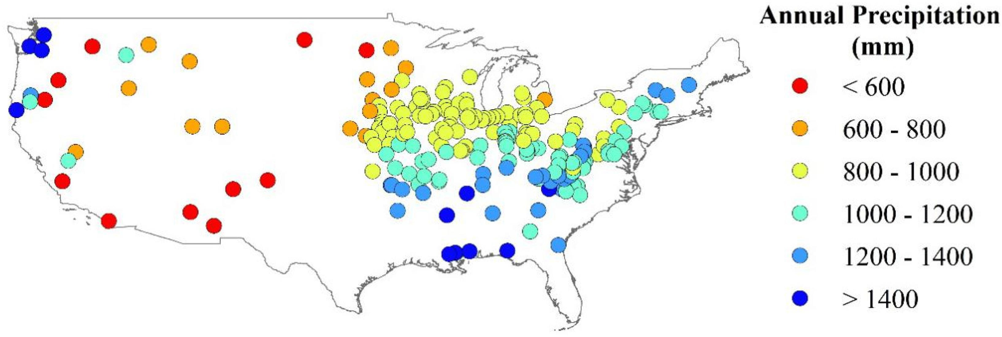
The 208 MOPEX basins (67 to 10,096 km2) used in this study are located in the continental United States with a diversity of climate characteristics, from semi-arid to temperate and tropical humid regions. Figure 1 shows the average annual precipitation (mm) for the 208 selected MOPEX basins, which varies greatly over the geographical region. Specifically, the precipitation is above 2000 mm on the west coast with temperate maritime climate, but less than 400 mm in arid regions in the central US with temperate continental climate and desert climate. Overall, average annual precipitation shows a clear east–west (subtropical humid climate zone, temperate continental climate zone, plateau mountain climate, and desert climate zone) gradient with decreasing values toward the west coast, and demonstrates another north–south (subtropical humid climate zone, temperate continental climate zone) gradient in the eastern U.S with increasing values toward the south coast.
2.1.2. Data Implementation
This study utilizes daily precipitation, ETP, runoff, and RS-ET data from 1983 to 2003 in the selected 208 MOPEX basins. Specifically, the calibration period is from 1983 to 1996 and the validation period is from 1997 to 2003. Data in the first 60 days are sacrificed for model warming-up.
2.2. Methodology
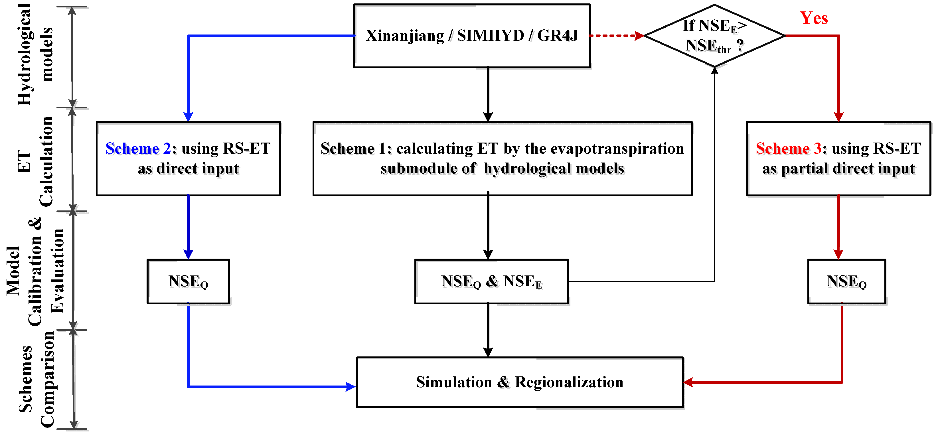
The schematic diagram of the methodology is shown in Figure 2. Three modeling schemes are implemented: (i) the original hydrological model with ET calculated by the respective evapotranspiration sub-module (Scheme 1); (ii) modification of the original models to use RS-ET data as direct input (Scheme 2); and (iii) modification of Scheme 2 to use RS-ET as partial direct input (Scheme 3) as it was later noted that using RS-ET as direct input could only improve the modeling results in some cases. Using the three RR models, these three schemes are compared to investigate a general practical method to improve runoff prediction in ungauged basins by using RS-ET data as direct input.
2.2.1. RR Models
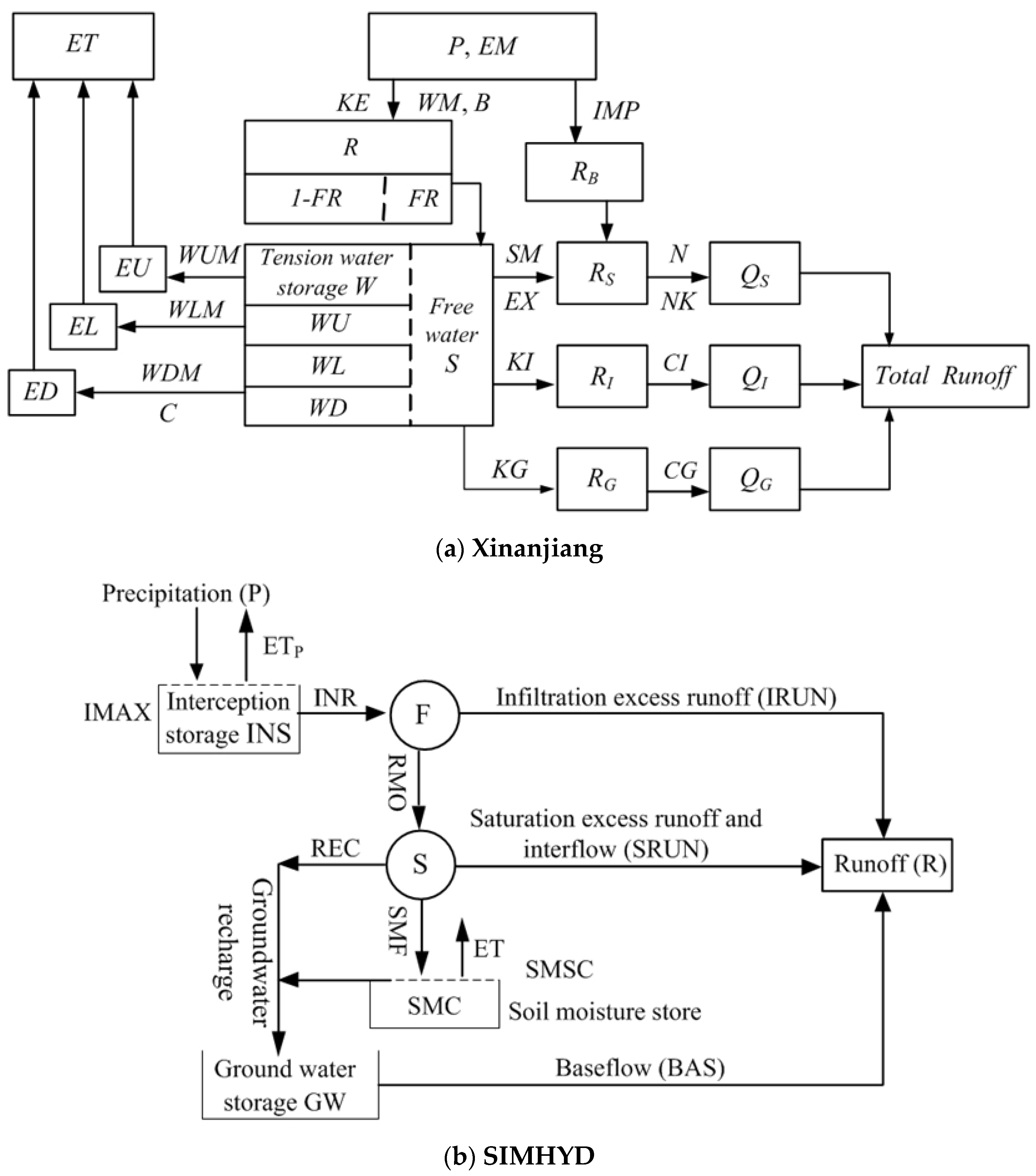
As shown in Table 1, most past studies used only one RR model, but the results were model dependent to some extent. To investigate the impact of model choice on RR modeling, several RR models are applied. RR models in this study are selected on the basis of several criteria. Firstly, lumped conceptual RR models are required because they have relatively simple structures and few parameters, and therefore can be easily regionalized to ungauged basins [18,27,37,38]. Secondly, RR models are required to be representative (i.e., have different model structures, different numbers of parameters, and different emphases on physical processes) and widely used for runoff prediction over different climatic areas. Finally, it is expected that inputs to the RR models are daily precipitation and ETP considering the availability of data materials in the study. Considering the above factors, three lumped conceptual RR models are selected, namely, Xinanjiang, GR4J, and SIMHYD. A schematic overview of the three RR models is presented in Figure 3.
- (1)
- Xinanjiang model
The Xinanjiang hydrological model is a conceptual RR model developed in 1995 [39] and has been widely used for hydrological forecasts since the 1980s. The Xinanjiang model has much emphasis on physical processes and relatively more parameters. A schematic diagram of the model structure is described in Figure 3a, which consists of four main sub-modules: (i) evapotranspiration, (ii) runoff production, (iii) runoff separation, and (iv) flow routing.
A three-layer soil moisture model is used to determine the actual evapotranspiration ET in the Xinanjiang model [42]. The evaporation of the upper layer EU occurs at the potential rate EP until the storage of the upper layer WU is exhausted.
Evapotranspiration of the lower layer EL is modeled as a multiplication function of the remaining potential evapotranspiration on exhaustion of the upper layer (EP − EU) and the actual storage WL of the lower layer.
Evapotranspiration of the deepest layer ED is modeled as a proportion C of the remaining potential evapotranspiration on exhaustion of the upper layer (EP − EU), and subtracting EL.
The total actual evapotranspiration ET is the sum of evapotranspiration from the three soil layers, i.e., ET = EU + EL + ED, where WU, WL, and WD are the areal mean tension water storage of the upper, lower, and deepest layer, and WUM, WLM, and WDM are the areal storage capacity of the upper, lower, and deepest layer, respectively.
- (2)
- SIMHYD
SIMHYD is a seven-parameter lumped conceptual daily RR model developed in 2002 [40]. The model represents physical processes by conceptual equations, and therefore consists of separate components for interception, infiltration excess runoff, saturation excess runoff/interflow, and baseflow. The structure of SIMHYD is presented in Figure 3b.
The total actual evapotranspiration ET in SIMHYD consists of interception evaporation and soil evapotranspiration. The former occurs at the potential rate ETP, and the latter is calculated as a linear function of the actual storage SMS.
- (3)
- GR4J
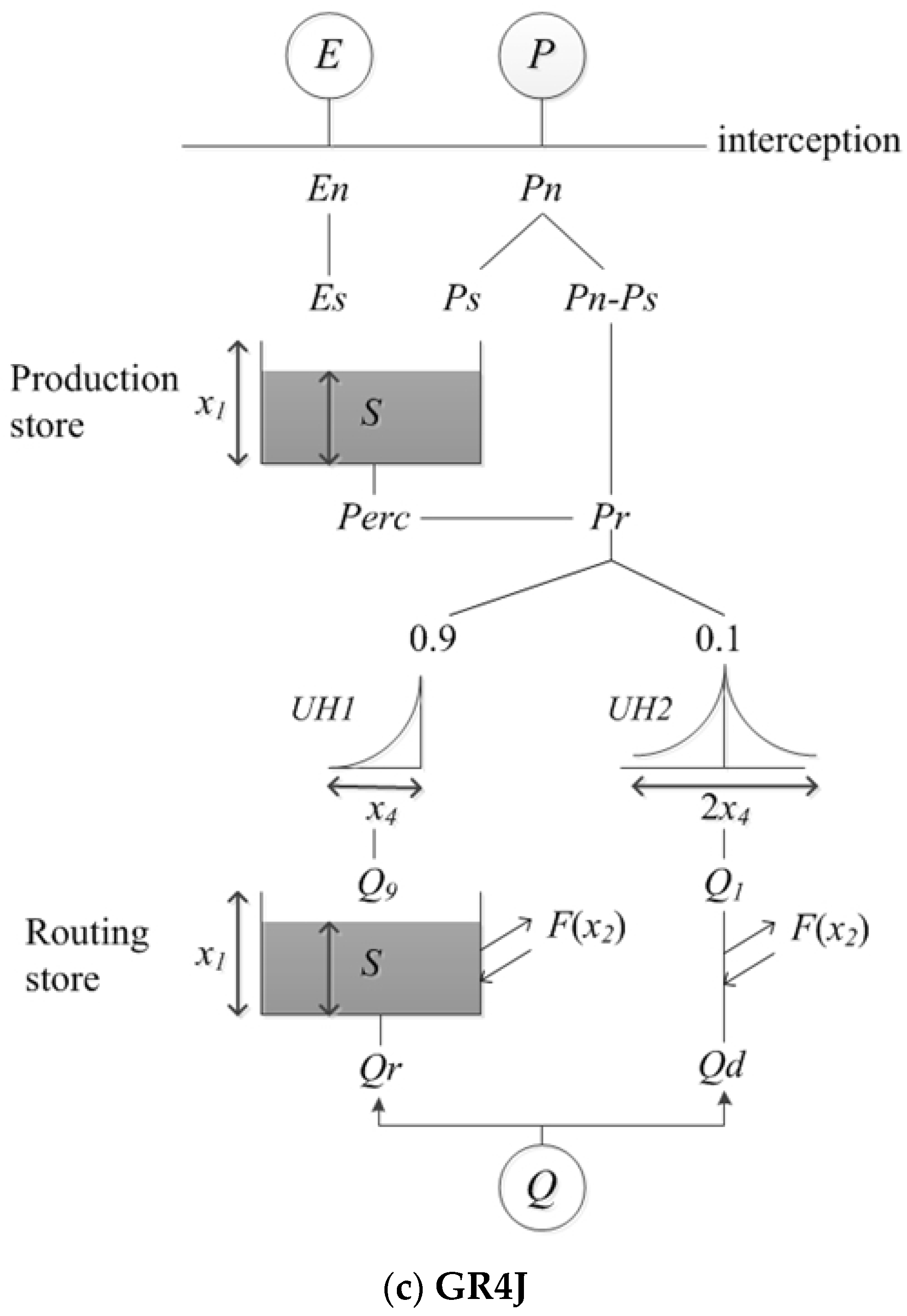
GR4J is a compact lumped RR model with four parameters [41,43]. The model structure is shown in Figure 3c, which was determined by the empirical match of multiple candidate structures with calibration data and therefore has less emphasis on physical processes.
The total actual evapotranspiration in GR4J model is calculated as a function of net evapotranspiration capacity (En) and the level S in the production storage. En is determined by subtracting ETP from precipitation.
where x1 (mm) is the maximum capacity of the production store.
2.2.2. Model Calibration, Regionalization, and Evaluation
- (1)
- Model calibration
Model parameters are estimated using the genetic algorithm [44], Rosenbrock method [45], and downhill simplex method [46] successively. Similar to other algorithms [47,48], such as the shuffled complex evolution method and estimation of distribution algorithm, the combined application of these three algorithms is sufficient to find the near-optimal parameters.
In each of the three schemes, model parameters are calibrated to match simulated streamflow to observed data following Equation (6). The objective function F is the multiplication of the mean square error (MSE) and the relative volume error between the observed and simulated streamflow. MSE is used to minimizes the simulation error of the discharge hydrographs, and the relative volume error ensures the overall balance of the total runoff volume.
where and are the observed and simulated discharges (m3 s−1) on the ith day, respectively; and n is the number of days.
- (2)
- Parameter regionalization
Parameter regionalization is conducted in 208 basins to evaluate runoff prediction in ungauged basins. Specifically, each basin is regarded as ‘ungauged’ in turn, and the runoff is modeled using the optimized parameter values from the ‘donor’ basin [3,49,50,51,52,53]. Runoff prediction results in ungauged basins are then evaluated using the spatial proximity method.
For each targeted ‘ungauged’ basin, the corresponding ‘donor’ basin is determined by the spatial proximity method, i.e., the geographically nearest gauged basin is selected as the ‘donor’ basin. The spatial proximity method [37,38] is based on geographical distance similarity. It has been demonstrated that the spatial proximity method can yield similar or even better results [2,11] compared with the more complex physical similarity method, which is based on physical attribute similarity [38,54].
- (3)
- Model evaluation
Two indicators are used to evaluate the modeling performance: Nash–Sutcliffe efficiency (NSE) [55], and the water balance index (WBI).
NSE measures how well the residual variance agrees with the observed variance. In this study, NSEQ and NSEE refer to the NSE value of discharge and ET, respectively:
where is the average observed discharge (m3 s−1); and are the RS and the simulated ET values (mm) on the ith day, respectively; is the average RS-ET (mm); n is the number of days. NSE ranges from −∞ to 1. The value of NSE should be positive, and higher values indicate better performance [56]. A value of zero for NSE indicates that the observed mean is as good as the model-simulated result, while negative values indicate that the observed mean is a better predictor than the model. Note that since the evapotranspiration sub-module is replaced directly by RS-ET data in Scheme 2 and Scheme 3, NSEE is calculated only in Scheme 1 to evaluate the ET simulation efficiency of the original RR models.
WBI indicates the relative volume error between the simulated and observed streamflow, which is calculated as in Equation (9). A value of zero for WBI means no bias, and a positive value indicates an overestimation of the total runoff volume and vice versa. Therefore, values closer to zero indicate better performance.
2.2.3. Modeling Scheme
Three modeling schemes are used here: Scheme 1 represents the conventional RR modeling method, while Scheme 2 and Scheme 3 use RS-ET as complete and partial direct input of RR models, respectively. All these three schemes are carried out for streamflow modeling in gauged basins and prediction in ungauged basins.
- (1)
- Scheme 1
Scheme 1 is the benchmark scheme, i.e., the conventional modeling method in which ET is simulated by the evapotranspiration sub-module of the original hydrological models. Consequently, streamflow and ET simulation are evaluated by NSEQ and NSEE, respectively.
- (2)
- Scheme 2
Scheme 2 is the method of using RS-ET as direct input in past studies (see Table 1). This scheme provides a second benchmark with no premise set about the utilization of RS-ET data. RS-ET is used to replace the evapotranspiration sub-module directly so that three RR models are slightly modified to accommodate RS-ET as direct input. Specifically, in the Xinanjiang model, the original three-layer evapotranspiration sub-module is simplified to a single layer and uses RS-ET directly, removing Equation (1) to Equation (3) and the four evapotranspiration parameters, WUM, WLM, KE, and C. Consequently, the modified Xinanjiang model has 11 parameters to be optimized. In SIMHYD and GR4J, the ET calculated by Equations (4) and (5) is replaced directly with RS-ET, and the model parameters remain the same as those in the original models.
- (3)
- Scheme 3
Scheme 3 is designed to use RS-ET data as partial direct input. The principle is to use RS-ET in cases where runoff prediction can be improved, i.e., where Scheme 2 outperforms Scheme 1.
The key of Scheme 3 is to identify the characteristics of cases where Scheme 2 surpasses Scheme 1. As shown in Table 1, although past studies implemented Scheme 2 over a variety of RS-ET data and lumped conceptual hydrological models, only a minority of these studies had improved streamflow modeling in gauged/ungauged basins [2,11,18,26]. The results of Scheme 2 can be attributed to the accuracy of RS-ET data, characteristics of catchment data, model structure, parameter optimization, etc. The hypothesis is that NSEE of Scheme 1 not only indicates the ET simulation efficiency of the original models, but also reflects the compatibility of model structure with RS-ET data and therefore affects the efficacy of using RS-ET. Accordingly, Scheme 3 utilizes RS-ET as direct input on the premise that NSEE of Scheme 1 exceeds the respective threshold values (NSEthr) of three RR models. Otherwise, on the condition that NSEE of Scheme 1 is below the NSEthr, RS-ET is not used and ET is modeled in the same way as in Scheme 1.
3. Results and Discussion
3.1. Conventional Streamflow Prediction
Table 2 presents the modeling and prediction performances of Scheme 1 over 208 MOPEX basins. For both model simulation in gauged basins and prediction in ungauged basins, the Xinanjiang model simulates both streamflow and ET efficiently, with the 50th percentile NSEE above 0.48. GR4J performs well for streamflow but poor for ET, with the 75th percentile NSEE below 0.2 and 50th percentile below 0.1, which results in a lower NSEE threshold of GR4J than that of Xinanjiang and SIMHYD models. For SIMHYD, the streamflow performance is the worst of three models, but the ET performance is between that of the above two models. Generally, SIMHYD simulates both streamflow and ET poorly, with the 75th percentile NSEQ below 0.5 and NSEE below 0.4. Generally, the relative performance of NSEQ is GR4J > Xinanjiang > SIMHYD, while in terms of NSEE, Xinanjiang > SIMHYD > GR4J. For all three models, the regionalization results in ungauged basins are worse than simulation results in gauged basins.
The efficient performances of both streamflow and ET simulation for the Xinanjiang model indicate its emphasis on both of these two processes. The three-layer soil moisture model has more flexibility than the one-layer sub-module in the SIMHYD and GR4J models, and may explain the favorable ET result. However, GR4J performs well for streamflow but poorly for ET simulation, probably because the parsimonious GR4J model is primarily designed for streamflow simulation [41]. In almost all cases, the accuracy of streamflow simulation is higher than that of ET. The RR models put the main emphasis on estimating runoff while having less emphasis on evapotranspiration processes [57]. Although ET is calculated to account for soil water balance, quantifying surface energy fluxes is not a focus in RR models.
3.2. Selection of RS-ET Utilization Threshold
The value of NSEthr is selected, considering two factors: (i) the relative superiority level (superior basin percent) of Scheme 2 over Scheme 1, and (ii) the number of basins for analysis (basins with NSEE values exceeding NSEthr). The former factor is determined by the representation of evapotranspiration processes in the RR model, and the latter is affected by the overall ET simulation performances of the model.
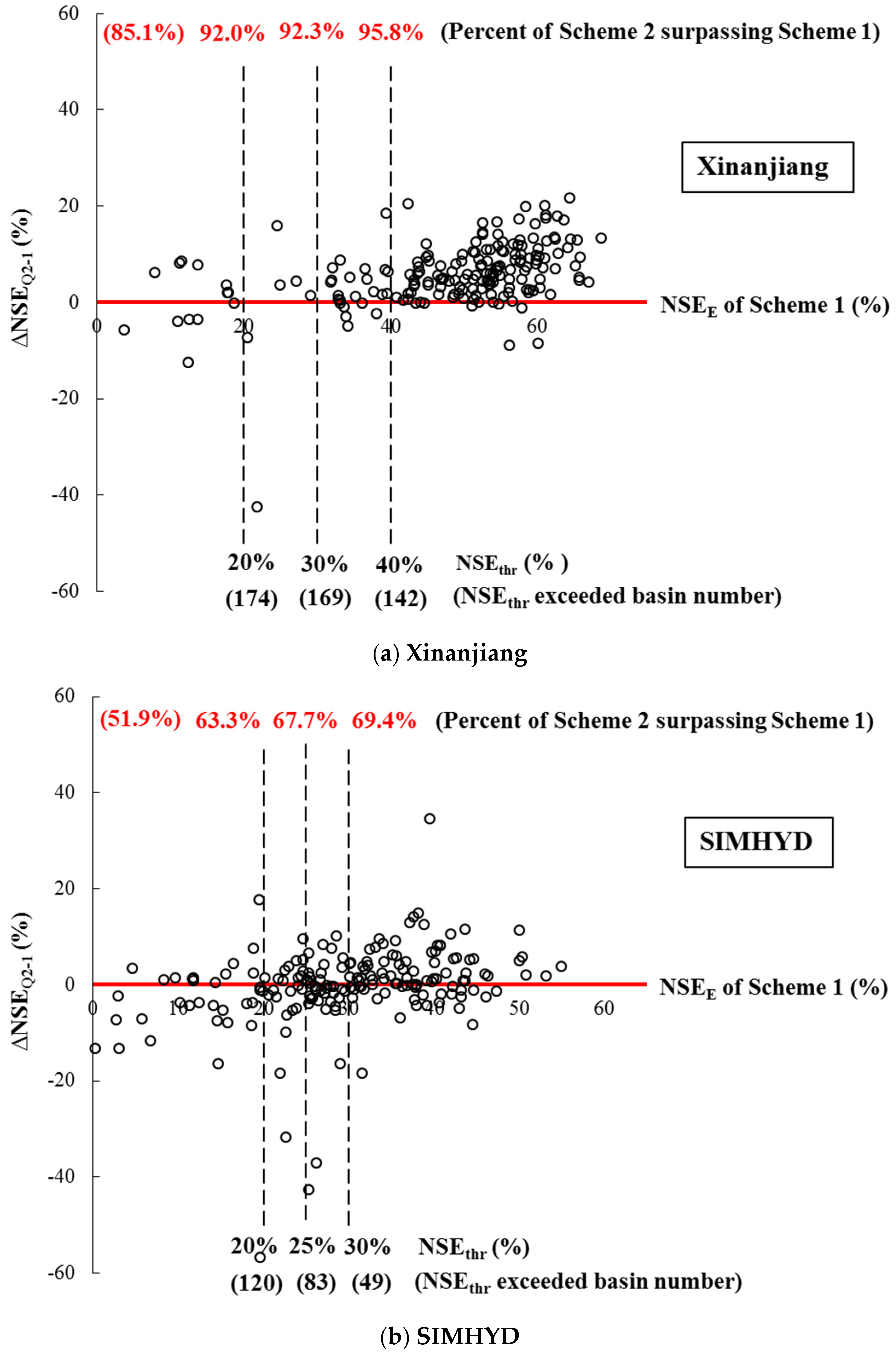
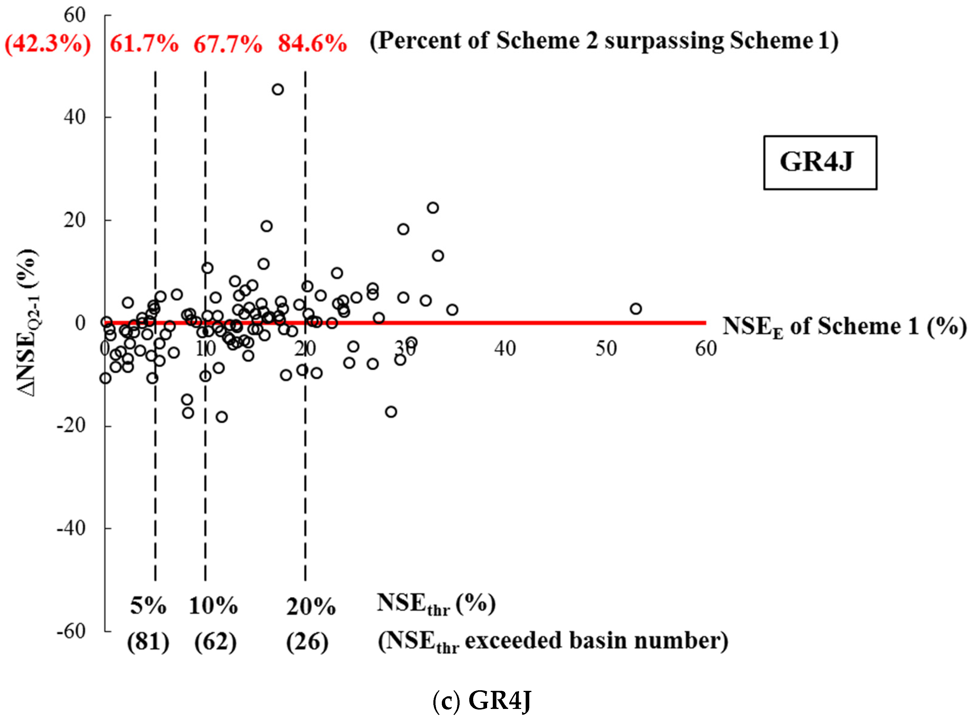
Figure 4 presents the results of streamflow simulation improvement using RS-ET as complete direct input over 208 gauged basins, and depicts the relationship of the relative performances between Scheme 2 and Scheme 1 (ΔNSEQ2-1 = NSEQ2 − NSEQ1) versus NSEE of Scheme 1 in the calibration period (the result in the validation period is similar and is therefore not presented here).
As shown in Figure 4a, for the Xinanjiang model, Scheme 2 outperforms Scheme 1 (ΔNSEQ2-1 > 0) in 85.1% of the total 208 basins. The NSEE of Scheme 1 exceeds the NSEthr values of 0.2, 0.3, and 0.4 in 174, 169, and 142 basins, respectively. It can be seen that Scheme 2 outperforms Scheme 1 in 92.0%, 92.3%, and 95.8% of the corresponding 174, 169, and 142 basins, respectively. Similar analysis is conducted for SIMHYD in Figure 4b, which shows that Scheme 2 outperforms Scheme 1 in 51.9% of the total 208 basins and the superiority is actually marginal. The NSEE of Scheme 1 exceeds the NSEthr values of 0.2, 0.25, and 0.3 in 120, 183, and 49 basins, of which the corresponding basin proportion of Scheme 2 surpassing Scheme 1 is 63.3%, 67.7%, and 69.4%, respectively. Similarly, for GR4J in Figure 4c, Scheme 2 outperforms Scheme 1 only in 42.3% of the total 208 basins, indicating that using RS-ET as direct input fails to improve model performance in most basins. However, Scheme 2 surpasses Scheme 1 in 61.7%, 67.7%, and 84.6% of the basins where the NSEE of Scheme 1 exceeds 0.05, 0.1, and 0.2, respectively. Generally, the superiority of using RS-ET over the conventional method is more significant with higher NSEthr values. In this vein, NSEE of Scheme 1 could be used as a measurement for acceptability of RS-ET data as direct input.
As shown in Figure 4, the relative performances of Scheme 2 versus Scheme 1 are different among three RR models. For Xinanjiang, NSEE of Scheme 1 exceeds 0.3 in 169 basins and Scheme 2 surpasses Scheme 1 for 92.3% of these basins. For SIMHYD, NSEE of Scheme 1 exceeds 0.25 in 83 basins and Scheme 2 surpasses Scheme 1 for 67.5% of these basins. For GR4J, NSEE of Scheme 1 exceeds 0.1 in 62 basins and Scheme 2 surpasses Scheme 1 for 67.7% of the basins. However, the relative superiority can be modest with lower NSEthr, and the number of basins (especially for GR4J) can be insufficient for analysis with higher NSEthr. Taking into account both the relative superiority level and the basin numbers for analysis, NSEE values of 0.3, 0.25, and 0.1 are eventually chosen as the NSEthr for the Xinanjiang, SIMHYD, and GR4J models, respectively.
3.3. Streamflow Prediction Using RS-ET
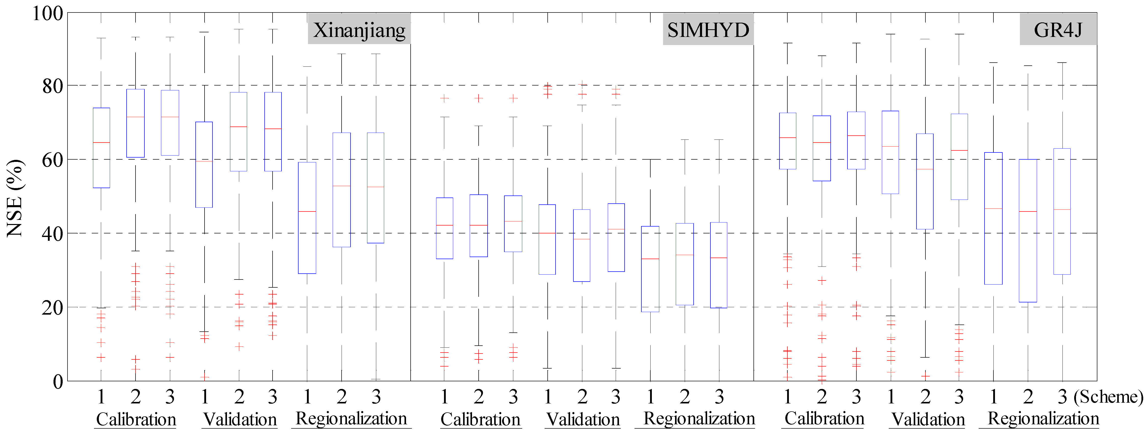
Figure 5 compares streamflow simulation performances of the three schemes for both the simulation and regionalization over 208 basins. It is clear that for all three modeling schemes, Xinanjiang and GR4J models perform better than SIMHYD. Compared with the results of simulation, the performances of all three RR models are worse in regionalization, with the median NSEQ values decreasing by approximately 0.1 compared with the results of validation. Moreover, the inter-quartile range (the spacing between edges of the box) is wider in regionalization, showing larger variability of NSEQ results. As for modeling schemes, Scheme 3 performs the best for both the simulation and regionalization. Specifically, Scheme 2 surpasses Scheme 1 significantly for the Xinanjiang model, but performs only slightly better or even worse than Scheme 1 for SIMHYD and GR4J models. The results indicate that using RS-ET data as direct input may not definitely improve streamflow simulation performances, which is consistent with the results of most past studies [12,58]. However, Scheme 3 outperformed both Scheme 1 and Scheme 2 almost in all cases, though more significantly for the Xinanjiang model than for the other two models. Generally, the performance differences between Scheme 2 and Scheme 3 are marginal, as inferred from Figure 5.
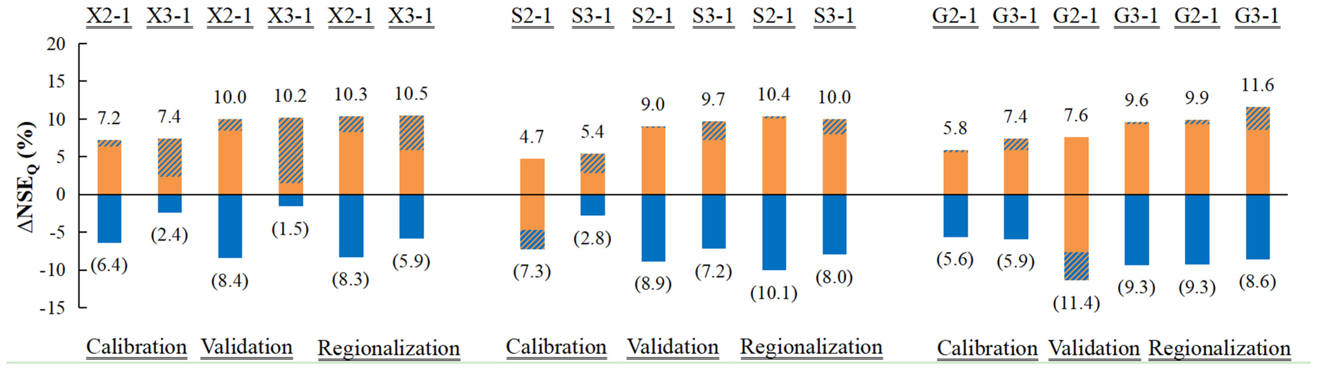
To further clarify the improvement/reduction in model performances by using RS-ET data, the average relative performances (ΔNSEQ) of Scheme 2 and Scheme 3 versus Scheme 1 are presented in Figure 6. For the Xinanjiang model, the magnitude of the NSEQ increase exceeds that of the NSEQ decline in all cases, i.e., the performance improvement dominates for both Scheme 2 and Scheme 3. For SIMHYD and GR4J, the improvement dominates in all cases for Scheme 3, but the net ΔNSEQ is relatively marginal. For all three RR models, the net performance improvement of Scheme 3 is more significant than that of Scheme 2, demonstrating the superiority of Scheme 3.
Furthermore, the frequency with which Scheme 2 and Scheme 3 surpass Scheme 1 is presented in Table 3. A comparison between Scheme 1 and Scheme 2 is conducted over all the 208 MOPEX basins. However, in Scheme 3, RS-ET data are used only if the NSEE of Scheme 1 exceeds the respective NSEthr. Accordingly, Scheme 3 using the Xinanjiang, SIMHYD, and GR4J models are compared with Scheme 1 over 169, 83, and 62 MOPEX basins, respectively. Results show that for all these models, Scheme 3 surpasses Scheme 2 for both simulation and regionalization. Note that Scheme 3 outperforms Scheme 1 in 91.1%, 59.0%, and 53.2% basins in regionalization for the Xinanjiang, SIMHYD and GR4J models, respectively, which indicates that using RS-ET data as partial direct input can improve streamflow prediction in most ungauged basins.
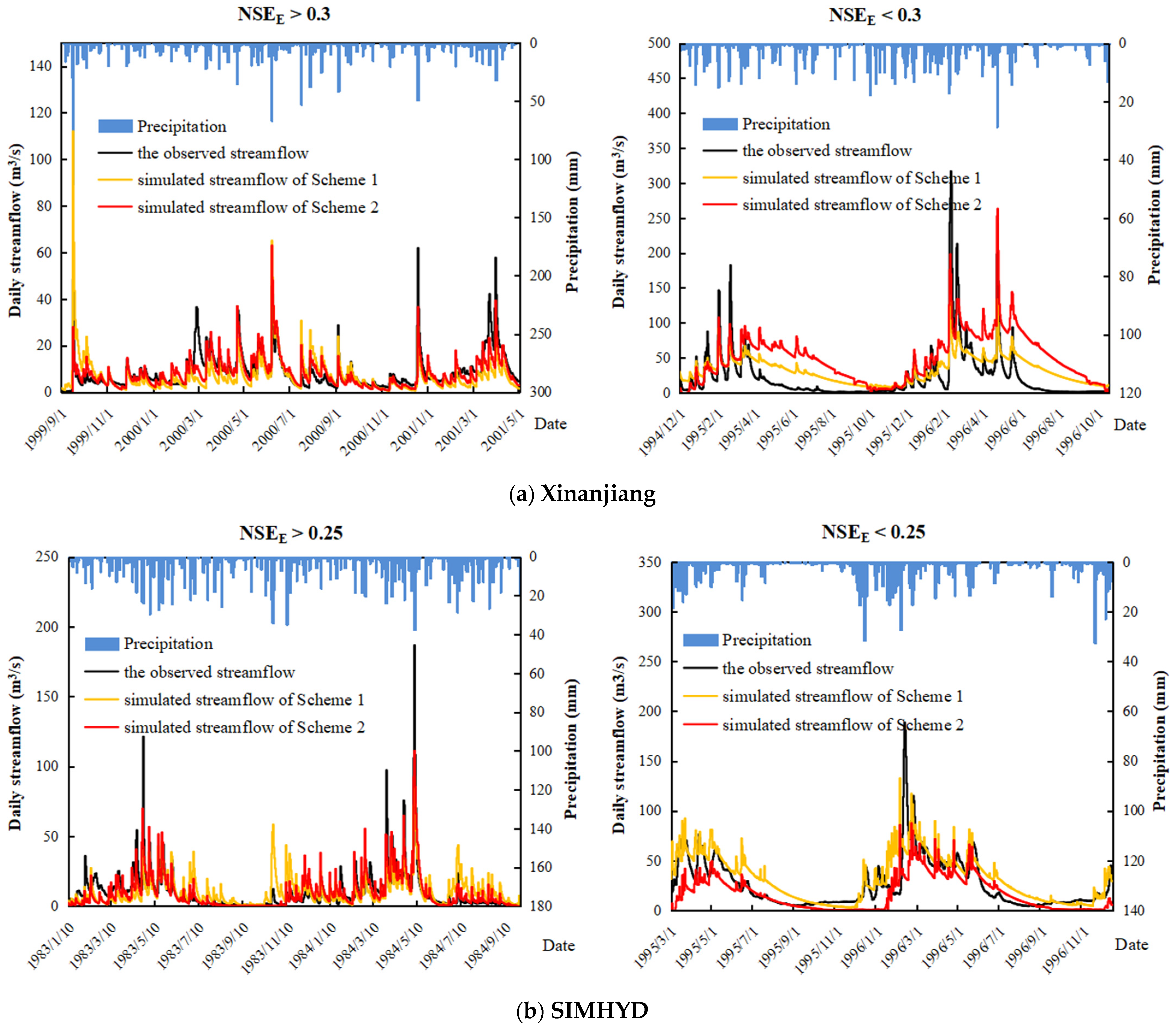
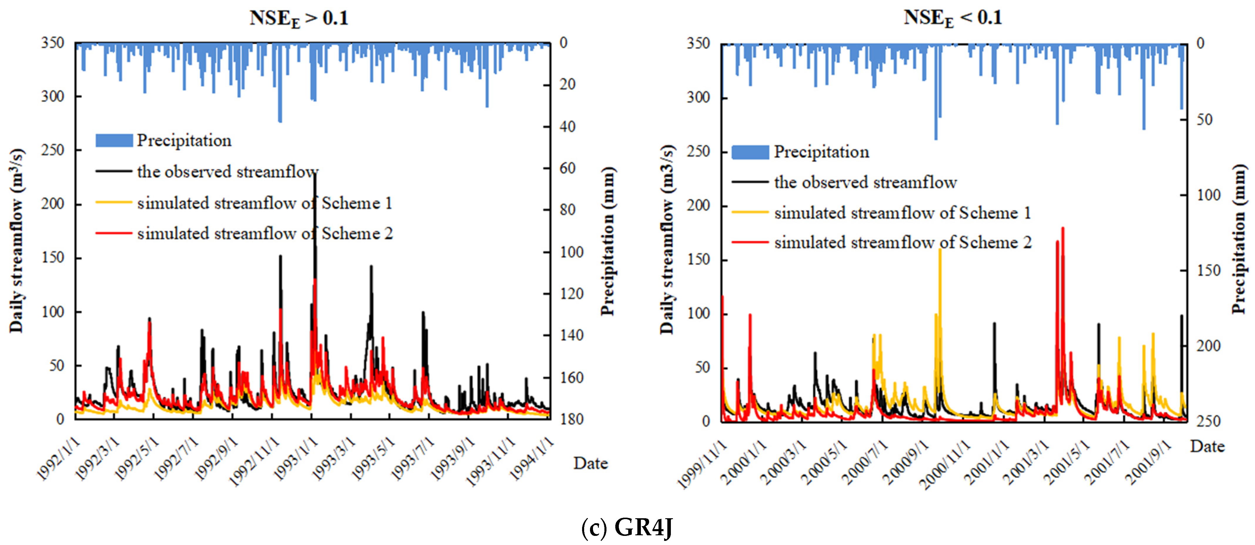
To verify the validity of the screening premise applied in Scheme 3 (NSEE of Scheme 1 is above the NSEthr) for streamflow prediction, Figure 7 compares simulated streamflow hydrographs between Scheme 1 and Scheme 2 in regionalization for the representative basins with NSEE > NSEthr and NSEE < NSEthr. It can be seen that for all three models, Scheme 2 simulates streamflow better than Scheme 1 in the basins with NSEE > NSEthr, but performs worse than Scheme 1 in the basins with NSEE < NSEthr. Specifically, in the basins with NSEE > NSEthr, both high flows and low flows are matched better in Scheme 2 than in Scheme 1. In the basins with NSEE < 0.3 for the Xinanjiang model, these two schemes perform similarly for high flows, but low flows are more overestimated in Scheme 2. In the basin with NSEE < 0.25 for the SIMHYD model, high flows are extremely underestimated in Scheme 2. In the basins with NSEE < 0.1 for the GR4J model, high flows are underestimated overall and are matched better in Scheme 1 than in Scheme 2. Therefore, Scheme 3, which uses RS-ET data provided that the NSEE of Scheme 1 exceeds the respective NSEthr, outperforms Scheme 1.
Generally, results show that using RS-ET for the improvement of streamflow prediction is most applicable and effective for the Xinanjiang model, which agrees with past studies [18,26]. The Xinanjiang emphasizes both streamflow and evapotranspiration processes and the evapotranspiration sub-module is relatively sophisticated, and may explain the favorable ET results and the efficacy of using RS-ET.
The GR4J model has the worst representation of the evapotranspiration process among the three models, which means the greatest incompatibility of the model structure with the RS-ET data. The SIMHYD model has a relatively better representation of evapotranspiration processes. However, the ET sub-module in SIMHYD is relatively simple. Consequently, SIMHYD is average in terms of performance and efficacy when using RS-ET. Furthermore, to replace the evapotranspiration sub-module with RS-ET data directly, all three RR models should be slightly modified. While the parameters in the SIMHYD and GR4J models remain the same as those of the original models, the four evapotranspiration parameters in the Xinanjiang model are removed, which therefore reduces parameter uncertainty. This may also contribute to the superiority of the Xinanjiang model for streamflow simulation improvement.
3.4. Water Balance Condition
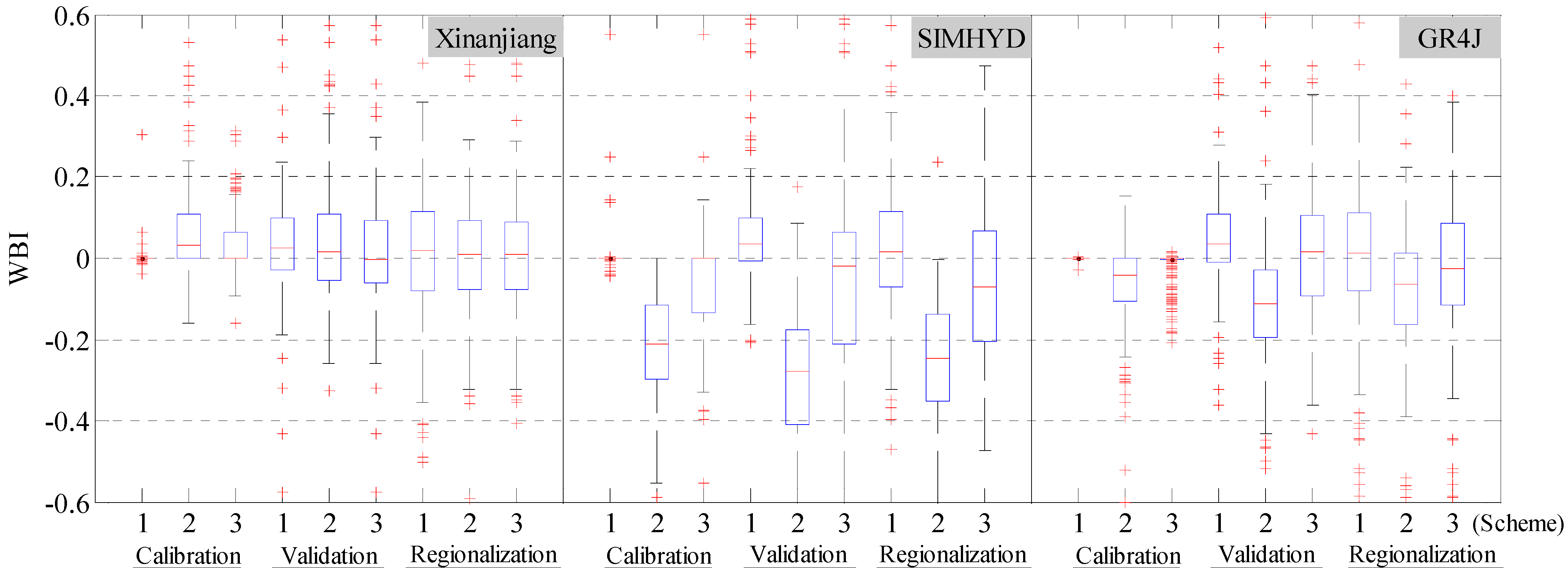
WBI is a basic factor for ensuring the water balance for hydrological simulation. Figure 8 compares the WBI values of the three schemes for both the simulation and regionalization over 208 basins. In all cases except Scheme 2 in the SIYHYD model, the median values of WBI range within ±0.1, which shows that the water balance condition is generally satisfactory. It is clear that the water balances of three models are similar for Scheme 1, while the Xinanjiang and GR4J models outperform the SIMHYD model for Scheme 2 and Scheme 3. Compared with the results of the simulation, the inter-quartile range of regionalization is wider, indicating a larger variability of WBI values in regionalization.
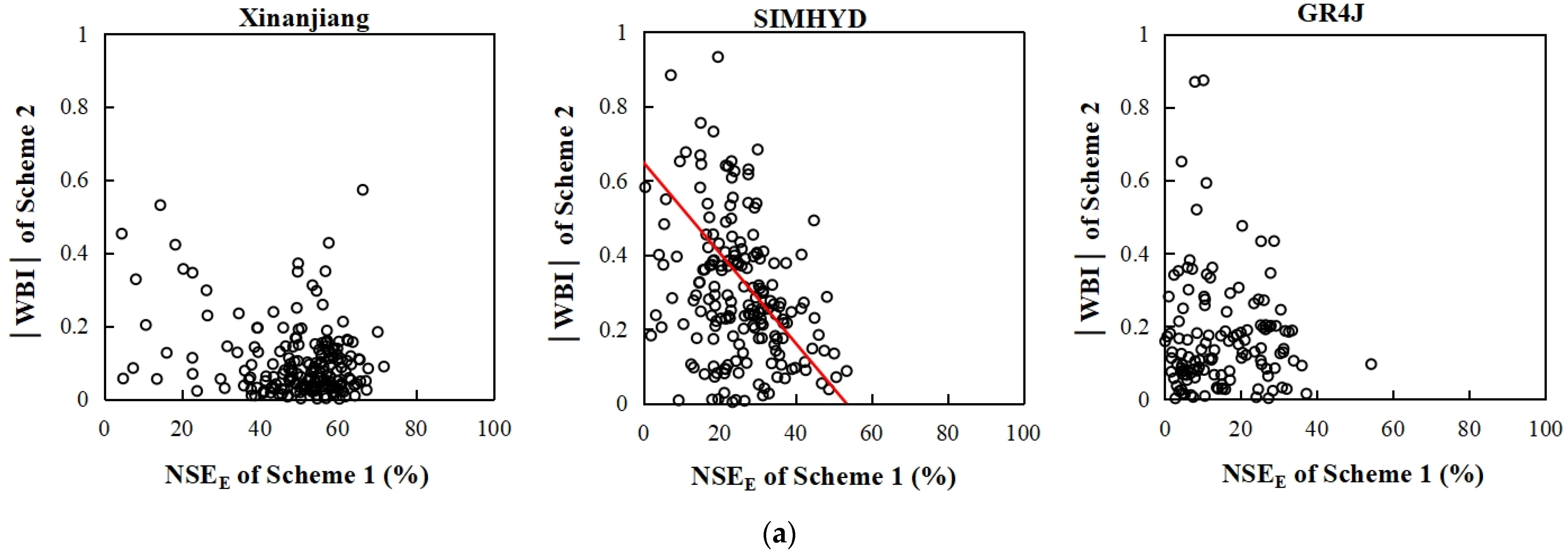
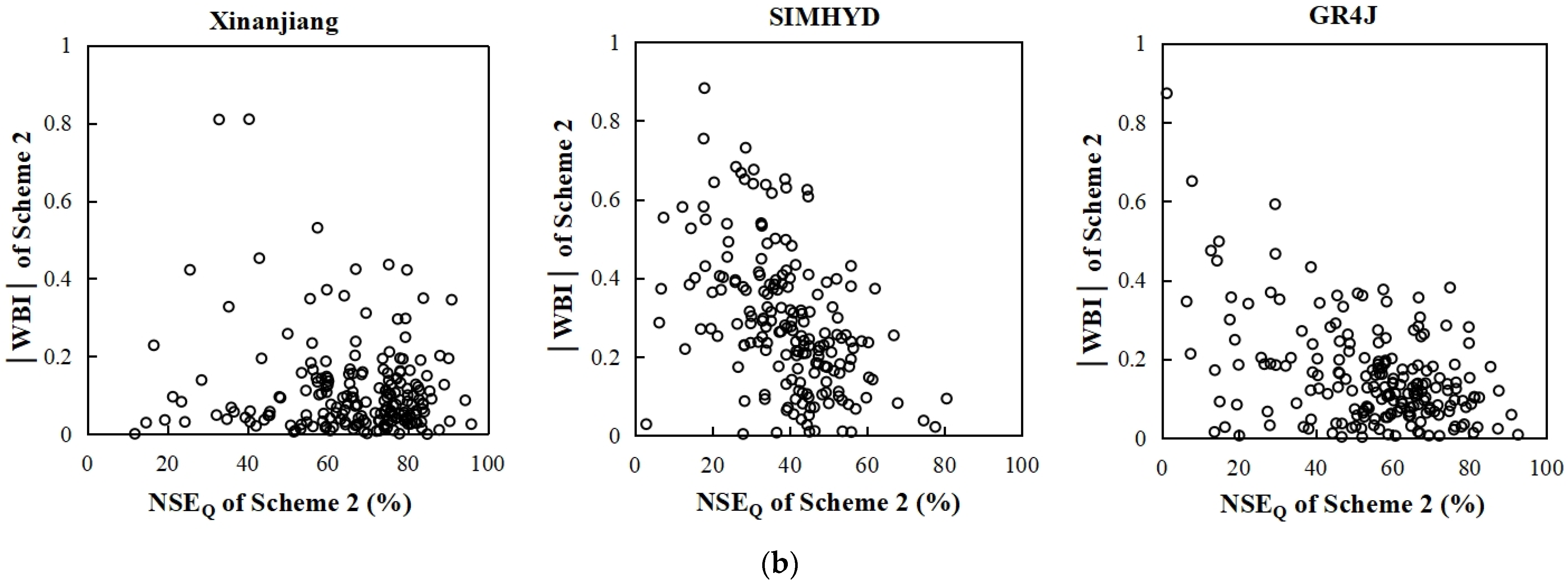
In all cases except the Xinanjiang model in regionalization, Scheme 1 performs the best for the water balance condition, whereas Scheme 2 performs the worst. Generally, using RS-ET as direct input weakens the estimation of the basin water balance, because the ET simulation is now fixed and cannot be used to correct the water balance error. In addition, the water balance of Scheme 3 is better than that of Scheme 2 in all cases, which could be attributed to the screening premise applied in Scheme 3 (NSEE of Scheme 1 is above the respective threshold). Figure 9a analyzes the relationship between WBI of Scheme 2 and NSEE of Scheme 1 in the validation period. Results demonstrate that the water balance based on RS-ET data is relatively better with the higher NSEE of Scheme 1, which explains the better WBI results of Scheme 3 compared to Scheme 2 in Figure 8. Furthermore, as inferred from the relationship between WBI and NSEQ results of Scheme 2 in Figure 9b, the NSEQ values of Scheme 2 are relatively higher, with better water balance results, which is consistent with the better streamflow performance of Scheme 3 compared to that of Scheme 2 in Figure 4.
Note that in regionalization, the water balance of Scheme 2 and Scheme 3 is better than that of Scheme 1 for the Xinanjiang model, but worse than that of Scheme 1 for SIMHYD and GR4J models, which indicates that using RS-ET only improves the water balance condition in the Xinanjiang model. The results can be attributed to the larger number of parameters in the Xinanjiang model, compared to the other models, to compensate for water balance errors.
3.5. Regional Spatial Patterns
It can be inferred from the above results that both complete and partial incorporation of RS-ET is more applicable for the Xinanjiang model. However, the performance of the SIMHYD model is relatively unsatisfactory, with the median NSEQ being below 0.45 for simulation and below 0.35 in regionalization, and the efficacy of using RS-ET is actually marginal for the GR4J model. Considering the heterogeneity in hydro-meteorological characteristics and evapotranspiration magnitudes over 208 study basins, the modeling results of the Xinanjiang model are analyzed from a geographical standpoint to reveal the regional spatial patterns.
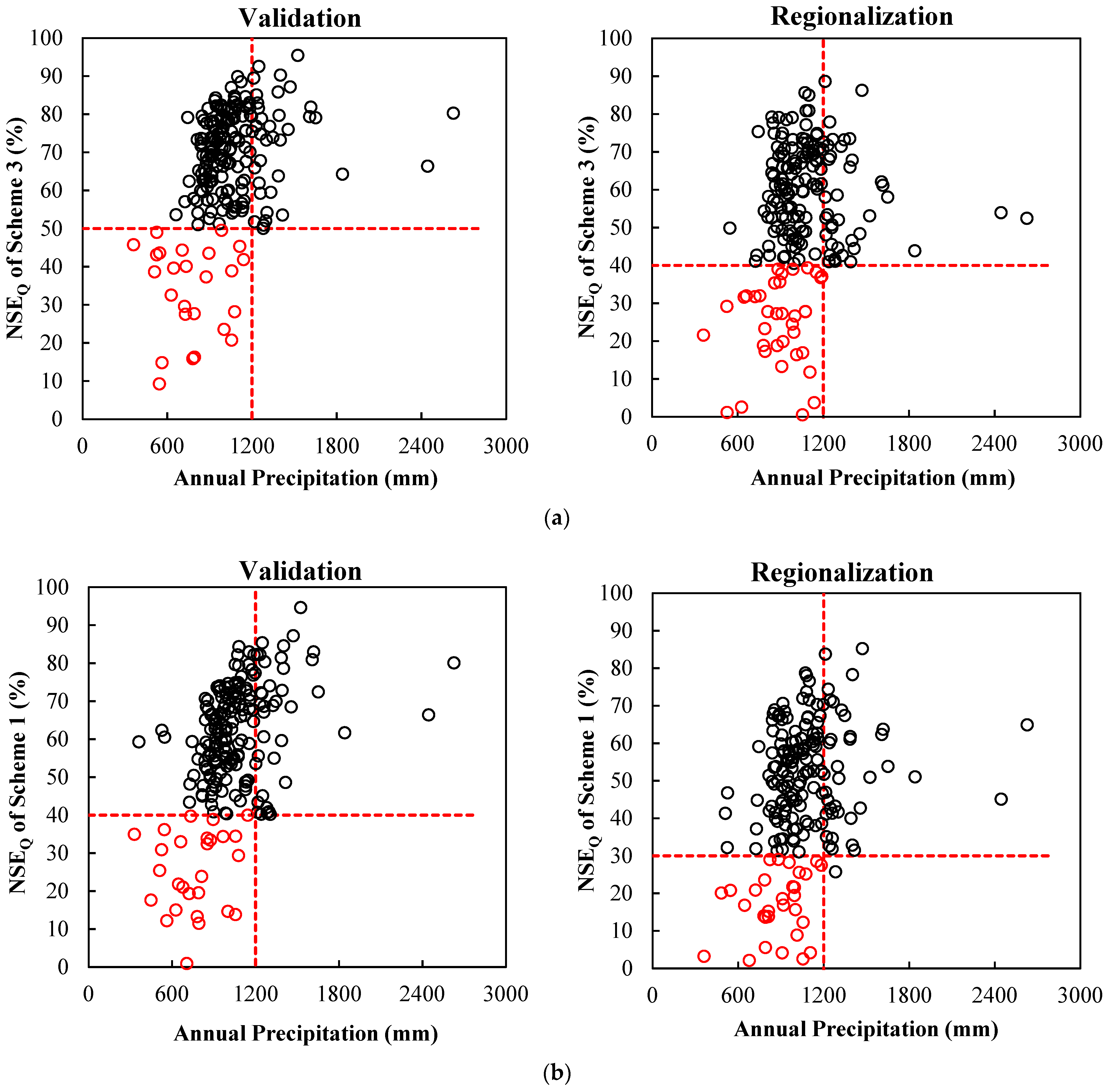
By comparing the NSEQ results of Scheme 3 with the average annual precipitation (mm) over 208 basins (Figure 1), there is a correlation between low precipitation values and poor model performances. The regional spatial pattern of Scheme 3 can be connected with the spatial pattern of the original Scheme 1 and the geographical characteristic of performance improvements by using RS-ET data. Figure 10 shows NSEQ in Scheme 3 and Scheme 1 versus the average annual precipitation (mm). It can be seen that there is a definite low-performance zone (NSEQ is below 0.5 in validation and below 0.4 in regionalization for Scheme 3, and NSEQ is below 0.4 in validation and below 0.3 in regionalization for Scheme 1) with annual precipitation below 1200 mm.
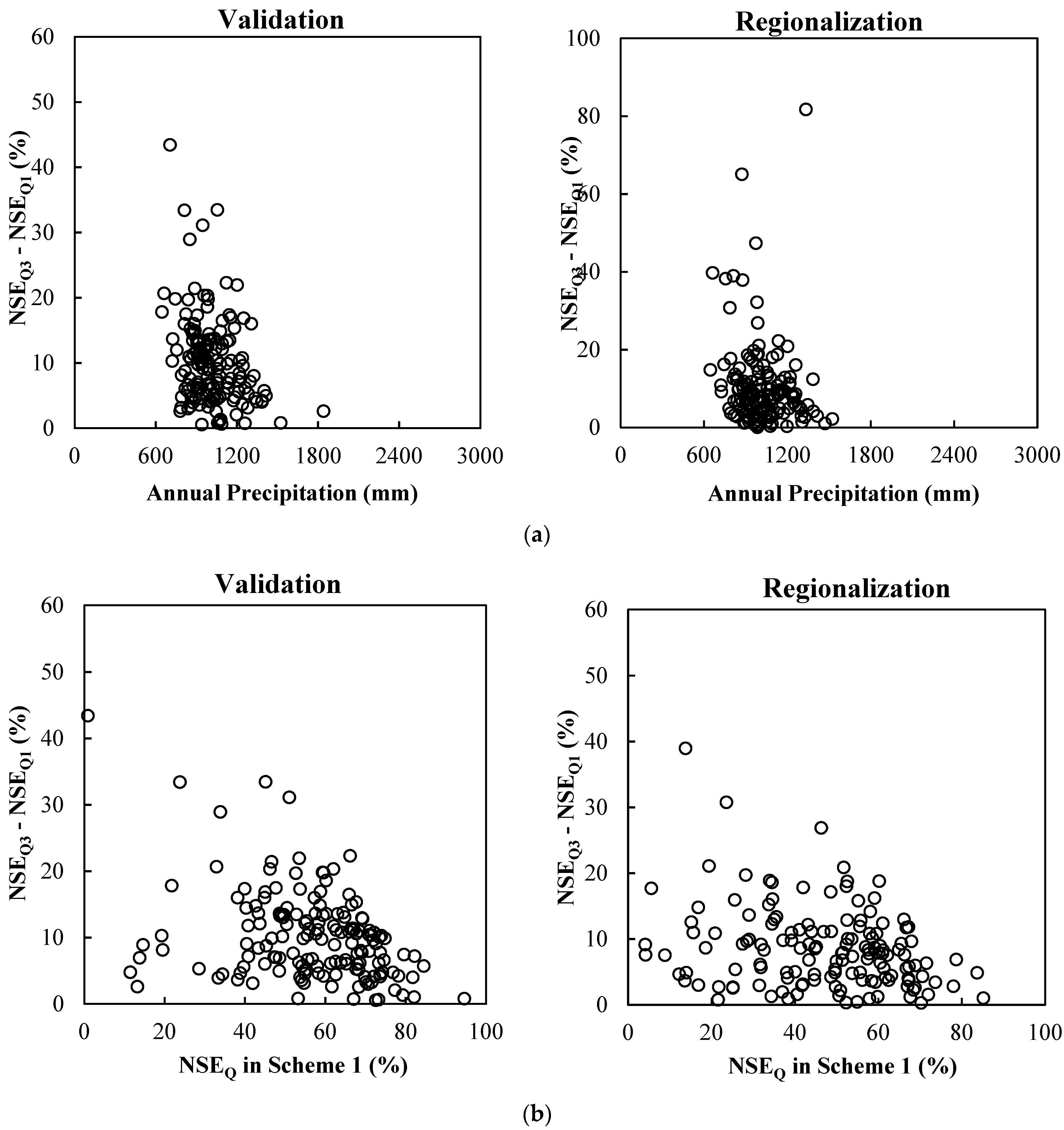
To further reveal the correlation between performance improvements and climatic regions, Figure 11 shows the relative performances between Scheme 3 and Scheme 1 (ΔNSEQ3-1 = NSEQ3 − NSEQ1) versus the average annual precipitation (mm). Positive ΔNSEQ3-1 indicates that Scheme 3 outperforms Scheme 1, and negative values indicate the opposite. It is noteworthy that higher ΔNSEQ3-1 values appear in basins that receive less than 1200 mm of annual precipitation. Results indicate that the performance-improved zone shown in Figure 11 coincides with the low-performance zone inferred from Figure 10. Accordingly, the correlation between the relative performances and the original performance of Scheme 1 is also analyzed in Figure 11, which demonstrates that the performance improvement is more significant in the originally poorly simulated basins.
In general, using RS-ET data improves runoff prediction in relatively arid and originally poorly simulated regions. The regional patterns are consistent with the results in Zhang et al. [27] and Kunnath-Poovakka et al. [13]. Basins in arid regions are water limited, where ET is constrained mainly by, and sensitive to, water supply. On the contrary, basins in humid regions are energy limited, where ET is constrained mainly by radiation and temperature [59,60]. The fact that in drier regions ET is more sensitive and exerts a more significant influence on water balance [61] could explain the success of schemes using RS-ET data in relatively arid areas. While some studies have shown streamflow improvement in humid regions [26], the regional patterns could also be related with the uncertainties of RS-ET data. Past studies demonstrated that the uncertainties of RS-ET in Zhang et al. [21] were larger in wet basins than in dry basins [62].
4. Conclusions
This study aims to develop a general practical method to improve runoff prediction in ungauged basins by using RS-ET data as a partial direct model input. Accordingly, in addition to the original RR models with ET calculated by the respective evapotranspiration sub-modules (Scheme 1), two methods of RS-ET inclusion are implemented: (1) modifying the original models to use RS-ET data as direct input (Scheme 2), and (2) using RS-ET as partial direct input provided that the ET simulation in Scheme 1 has acceptable accuracy (Scheme 3). These three schemes are compared in 208 MOPEX basins using three RR models and RS-ET data estimated from AVHRR. Runoff prediction results in ungauged basins are then evaluated by the spatial proximity method. By comparing the results of three schemes, conclusions and implications are drawn as follows:
(i) Using RS-ET as direct input improved model performances for the Xinanjiang model in over 85% basins, while worsening runoff prediction in most cases for the SIMHYD and GR4J models.
(ii) Further model improvements are obtained by using RS-ET as partial direct input, and are achieved in 91.1%, 59.0%, and 53.2% of basins for Xinanjiang, SIMHYD, and GR4J models, respectively.
(iii) Incorporation of RS-ET is more applicable for the Xinanjiang model, while less so for the GR4J model, and the efficacy is superior for basins that are relatively arid and originally poorly simulated.
Overall, using RS-ET as partial direct input is recommended, i.e., to test first whether the simulated ET from a particular hydrological model matches the RS-ET data well. If this is true, then the RS-ET data may be used as direct input in the model. It should be noted that the model performance is affected by the accuracy of RS-ET data and the variety of available RS data. Therefore, further development of RS technology and application of multi-source RS data can contribute to more efficient runoff prediction.
Author Contributions
Conceptualization, Z.G. and H.W.; Methodology, Z.G.; Software, F.Z. and A.X.; Validation, D.C.; Formal analysis, F.Z.; Investigation, D.C.; Resources, F.Z. and K.Y.; Data curation, D.C.; Writing—original draft, Z.G.; Writing—review & editing, A.X., K.Y. and H.W.; Funding acquisition, K.Y. All authors have read and agreed to the published version of the manuscript.
Funding
This study was supported by the Key Research and Development Program of Hubei Province (2020BCA073) and Wuhan Science and Technology Plan Project (2021WHYCQN-08).
Conflicts of Interest
The authors declare no conflict of interest.
References
- Sivapalan, M.; Takeuchi, K.; Franks, S.W.; Zehe, E. IAHS Decade on Predictions in Ungauged Basins (PUB), 2003–2012: Shaping an exciting future for the hydrological sciences. Hydrol. Sci. J. 2003, 48, 857–880. [Google Scholar] [CrossRef]
- Zhang, Y.; Chiew, F.H.S. Relative merits of different methods for runoff predictions in ungauged catchments. Water Resour. Res. 2009, 45, W07412. [Google Scholar] [CrossRef]
- Guo, Y.; Zhang, Y.; Zhang, L.; Wang, Z. Regionalization of hydrological modeling for predicting streamflow in ungauged catchments: A comprehensive review. Wiley Interdiscip. Rev. Water 2020, 8, e1487. [Google Scholar] [CrossRef]
- Yang, X.; Li, F.; Qi, W.; Zhang, M.; Xu, C.Y. Regionalization methods for PUB: A comprehensive review of progress after the PUB decade. Hydrol. Res. 2023, 54, 885–900. [Google Scholar] [CrossRef]
- Lakshmi, V. The role of satellite remote sensing in the Prediction of Ungauged Basins. Hydrol. Process. 2004, 18, 1029–1034. [Google Scholar] [CrossRef]
- Yoon, H.N.; Marshall, L.; Sharma, A.; Kim, S. Bayesian Model Calibration Using Surrogate Streamflow in Ungauged Catchments. Water Resour. Res. 2022, 58, e2021WR031287. [Google Scholar] [CrossRef]
- Hrachowitz, M.; Savenije, H.H.G.; Blschl, G.; Mcdonnell, J.J.; Cudennec, C. A decade of Predictions in Ungauged Basins (PUB)—A review. Hydrol. Sci. J. 2013, 58, 1198–1255. [Google Scholar] [CrossRef]
- Dembélé, M.; Ceperley, N.; Zwart, S.J.; Salvadore, E.; Mariethoz, G.; Schaefli, B. Potential of satellite and reanalysis evaporation datasets for hydrological modelling under various model calibration strategies. Adv. Water. Res. 2020, 143, 103667. [Google Scholar] [CrossRef]
- Guo, D.; Westra, S.; Maier, H.R. Impact of evapotranspiration process representation on runoff projections from conceptual rainfall-runoff models. Water Resour. Res. 2017, 53, 435–454. [Google Scholar] [CrossRef]
- Xu, Z.; Wu, Z.; Shao, Q.; He, H.; Guo, X. A two-step calibration framework for hydrological parameter regionalization based on streamflow and remote sensing evapotranspiration. J. Hydrol. 2022, 613, 128320. [Google Scholar] [CrossRef]
- Zhang, Y.; Chiew, F.H.S.; Zhang, L.; Li, H. Use of Remotely Sensed Actual Evapotranspiration to Improve Rainfall–Runoff Modeling in Southeast Australia. J. Hydrometeorol. 2009, 10, 969–980. [Google Scholar] [CrossRef]
- Vervoort, R.W.; Miechels, S.F.; Ogtrop, F.F.V.; Guillaume, J.H.A. Remotely sensed evapotranspiration to calibrate a lumped conceptual model: Pitfalls and opportunities. J. Hydrol. 2014, 519, 3223–3236. [Google Scholar] [CrossRef]
- Kunnath-Poovakka, A.; Ryu, D.; Renzullo, L.J.; George, B. The efficacy of calibrating hydrologic model using remotely sensed evapotranspiration and soil moisture for streamflow prediction. J. Hydrol. 2016, 535, 509–524. [Google Scholar] [CrossRef]
- Gui, Z.; Liu, P.; Cheng, L.; Guo, S.; Wang, H.; Zhang, L. Improving runoffff prediction using remotely sensed actual evapotranspiration during rainless periods. J. Hydrol. Eng. 2019, 24, 04019050.1–04019050.12. [Google Scholar] [CrossRef]
- Herman, M.R.; Nejadhashemi, A.P.; Abouali, M.; Hernandez-Suarez, J.S.; Daneshvar, F.; Zhang, Z.; Anderson, M.C.; Sadeghi, A.M.; Hain, C.R.; Sharifi, A. Evaluating the role of evapotranspiration remote sensing data in improving hydrological modeling predictability. J. Hydrol. 2018, 556, 39–49. [Google Scholar] [CrossRef]
- Yang, Y.; Guan, K.; Peng, B.; Pan, M.; Franz, T.E. High-resolution spatially explicit land surface model calibration using field-scale satellite-based daily evapotranspiration product. J. Hydrol. 2020, 596, 125730. [Google Scholar] [CrossRef]
- Zhang, L.; Zhao, Y.; Ma, Q.; Wang, P.; Ge, Y.; Yu, W. A parallel computing-based and spatially stepwise strategy for constraining a semi-distributed hydrological model with streamflow observations and satellite-based evapotranspiration. J. Hydrol. 2021, 599, 126359. [Google Scholar] [CrossRef]
- Li, H.; Zhang, Y.; Chiew, F.H.S.; Xu, S. Predicting runoff in ungauged catchments by using Xinanjiang model with MODIS leaf area index. J. Hydrol. 2009, 370, 155–162. [Google Scholar] [CrossRef]
- Taconet, O.; Bernard, R.; Vidal-Madjar, D. Evapotranspiration over an Agricultural Region Using a Surface Flux/Temperature Model Based on NOAA-AVHRR Data. J. Clim. Appl. Meteorol. 1986, 25, 284–307. [Google Scholar] [CrossRef]
- Nemani, R.R.; Running, S.W. Estimation of regional surface resistance to evapotranspiration from NDVI and Thermal-IR AVHRR data. J. Appl. Meteorol. 1989, 28, 276–284. [Google Scholar] [CrossRef]
- Zhang, K.; Kimball, J.S.; Nemani, R.R.; Running, S.W. A continuous satellite-derived global record of land surface evapotranspiration from 1983 to 2006. Water Resour. Res. 2010, 46, 109–118. [Google Scholar] [CrossRef]
- Cleugh, H.A.; Leuning, R.; Mu, Q.; Running, S.W. Regional evaporation estimates from flux tower and MODIS satellite data. Remote Sens. Environ. 2007, 106, 285–304. [Google Scholar] [CrossRef]
- Leuning, R.; Zhang, Y.Q.; Rajaud, A.; Cleugh, H.; Tu, K. A simple surface conductance model to estimate regional evaporation using MODIS leaf area index and the Penman-Monteith equation. Water Resour. Res. 2008, 44, 652–655. [Google Scholar] [CrossRef]
- Zhang, Y.Q.; Chiew, F.H.S.; Zhang, L.; Leuning, R.; Cleugh, H.A. Estimating catchment evaporation and runoff using MODIS leaf area index and the Penman-Monteith equation. Water Resour. Res. 2008, 44, 2183–2188. [Google Scholar] [CrossRef]
- Guerschman, J.P.; Van Dijk, A.I.J.M.; Mattersdorf, G.; Beringer, J.; Hutley, L.B.; Leuning, R.; Pipunic, R.C.; Sherman, B.S. Scaling of potential evapotranspiration with MODIS data reproduces flux observations and catchment water balance observations across Australia. J. Hydrol. 2009, 369, 107–119. [Google Scholar] [CrossRef]
- Zhou, Y.; Zhang, Y.; Vaze, J.; Lane, P.; Xu, S. Improving runoff estimates using remote sensing vegetation data for bushfire impacted catchments. Agr. Forest. Meteorol. 2013, 182–183, 332–341. [Google Scholar] [CrossRef]
- Zhang, Y.Q.; Vaze, J.; Chiew, F.H.S.; Liu, Y. Incorporating vegetation time series to improve rainfall-runoff model predictions in gauged and ungauged catchments. In Proceedings of the 19th International Congress on Modelling and Simulation, Perth, Australia, 12–16 December 2011. [Google Scholar]
- Szilagyi, J. Application of MODIS-Based Monthly Evapotranspiration Rates in Runoff Modeling: A Case Study in Nebraska, USA. Open J. Mod. Hydrol. 2013, 3, 172–178. [Google Scholar] [CrossRef]
- Roy, T.; Gupta, H.V.; Serrat-Capdevila, A.; Valdes, J.B. Using satellite-based evapotranspiration estimates to improve the structure of a simple conceptual rainfall and -runoff model. Hydrol. Earth Syst. Sci. 2017, 21, 879–896. [Google Scholar] [CrossRef]
- Duan, Q.; Schaake, J.; Andréassian, V.; Franks, S.; Goteti, G.; Gupta, H.V.; Gusev, Y.M.; Habets, F.; Hall, A.; Hay, L. Model parameter estimation experiment (MOPEX): An overview of science strategy and major results from the second and third workshops. J. Hydrol. 2006, 320, 3–17. [Google Scholar] [CrossRef]
- Jung, M.; Reichstein, M.; Ciais, P.; Seneviratne, S.I.; Sheffield, J.; Goulden, M.L.; Bonan, G.; Cescatti, A.; Chen, J.; de Jeu, R.; et al. Recent decline in the global land evapotranspiration trend due to limited moisture supply. Nature 2010, 467, 951–954. [Google Scholar] [CrossRef]
- Miralles, D.G.; Holmes, T.R.H.; De Jeu, R.A.M.; Gash, J.H.; Meesters, A.G.C.A.; Dolman, A.J. Global land-surface evaporation estimated from satellite-based observations. Hydrol. Earth Syst. Sci. 2010, 7, 453–469. [Google Scholar] [CrossRef]
- Vicente-Serrano, S.M.; Beguería, S.; López-Moreno, J.I. Comment on “Characteristics and trends in various forms of the Palmer Drought Severity Index (PDSI) during 1900–2008” by Aiguo Dai. J. Geophys. Res. 2011, 116, D19112. [Google Scholar] [CrossRef]
- Mátyás, C.; Sun, G. Forests in a water limited world under climate change. Environ. Res. Lett. 2014, 9, 085001. [Google Scholar] [CrossRef]
- Wang, D.; Alimohammadi, N. Responses of annual runoff, evaporation, and storage change to climate variability at the watershed scale. Water Resour. Res. 2012, 48, W05546. [Google Scholar] [CrossRef]
- Chen, X.; Alimohammadi, N.; Wang, D. Modeling interannual variability of seasonal evaporation and storage change based on the extended Budyko framework. Water Resour. Res. 2013, 49, 6067–6078. [Google Scholar] [CrossRef]
- Merz, R.; Blöschl, G. Regionalisation of catchment model parameters. J. Hydrol. 2004, 287, 95–123. [Google Scholar] [CrossRef]
- Oudin, L.; Andréassian, V.; Perrin, C.; Michel, C.; Le Moine, N. Spatial proximity, physical similarity, regression and ungaged catchments: A comparison of regionalization approaches based on 913 French catchments. Water Resour. Res. 2008, 44, W03413. [Google Scholar] [CrossRef]
- Zhao, R.J.; Liu, X.R.; Singh, V.P. The Xinanjiang model. In Computer Models of Watershed Hydrology; Singh, V.P., Ed.; Water Resources Publications: Littleton, CO, USA, 1995; pp. 371–381. [Google Scholar]
- Chiew, F.H.S.; Peel, M.C.; Western, A.W.; Singh, V.; Frevert, D. Application and testing of the simple rainfall-runoff model SIMHYD. In Mathematical Models of Small Watershed Hydrology and Applications; Water Resources Publication: Littleton, CO, USA, 2002; pp. 335–367. [Google Scholar]
- Perrin, C.; Michel, C.; Andréassian, V. Improvement of a parsimonious model for streamflow simulation. J. Hydrol. 2003, 279, 275–289. [Google Scholar] [CrossRef]
- Zhao, R.J. The Xinanjiang model applied in China. J. Hydrol. 1992, 135, 371–381. [Google Scholar] [CrossRef]
- Edijatno; Nascimento, N.D.O.; Yang, X.; Makhlouf, Z.; Michel, C. GR3J: A daily watershed model with three free parameters. Hydrol. Sci. J. 1999, 44, 263–277. [Google Scholar] [CrossRef]
- Goldberg, D.E. Genetic Algorithms in Search, Optimization, and Machine Learning; Addison-Wesley: Reading, MA, USA, 1989. [Google Scholar]
- Rosenbrock, H.H. An Automatic Method for Finding the Greatest or Least Value of a Function. Comput. J. 1960, 3, 175–184. [Google Scholar] [CrossRef]
- Nelder, J.A.; Mead, R. A simplex method for function minimization. Comput. J. 1965, 7, 308–313. [Google Scholar] [CrossRef]
- Duan, Q.; Sorooshian, S.; Gupta, V. Effective and efficient global optimization for conceptual rainfall-runoff models. Water Resour. Res. 1992, 28, 1015–1031. [Google Scholar] [CrossRef]
- Li, Z.; Liu, P.; Deng, C.; Guo, S.; He, P.; Wang, C. Evaluation of Estimation of Distribution Algorithm to Calibrate Computationally Intensive Hydrologic Model. J. Hydrol. Eng. 2016, 21, 04016012. [Google Scholar] [CrossRef]
- Kittel, C.M.M.; Arildsen, A.L.; Dybkjr, S.; Hansen, E.R.; Bauer-Gottwein, P. Informing hydrological models of poorly gauged river catchments—A parameter regionalization and calibration approach. J. Hydrol. 2020, 587, 124999. [Google Scholar] [CrossRef]
- Yang, X.; Magnusson, J.; Huang, S.; Beldring, S.; Xu, C.Y. Dependence of regionalization methods on the complexity of hydrological models in multiple climatic regions. J. Hydrol. 2019, 582, 124357. [Google Scholar] [CrossRef]
- Yang, X.; Magnusson, J.; Xu, C.Y. Transferability of regionalization methods under changing climate. J. Hydrol. 2018, 568, 67–81. [Google Scholar] [CrossRef]
- Arsenault, R.; Breton-Dufour, M.; Poulin, A.; Dallaire, G.; Romero-Lopez, R. Streamflow prediction in ungauged basins: Analysis of regionalization methods in a hydrologically heterogeneous region of Mexico. Hydrol. Sci. J. J. Des Sci. Hydrol. 2019, 64, 1297–1311. [Google Scholar] [CrossRef]
- Beck, H.E.; Pan, M.; Lin, P.; Seibert, J.; Dijk, A.I.J.M.V.; Wood, E.F. Global Fully Distributed Parameter Regionalization Based on Observed Streamflow From 4229 Headwater Catchments. J. Geophys. Res. Atmos. 2020, 125, e2019JD031485. [Google Scholar] [CrossRef]
- Young, A.R. Stream flow simulation within UK ungauged catchments using a daily rainfall-runoff model. J. Hydrol. 2006, 320, 155–172. [Google Scholar] [CrossRef]
- Nash, J.E.; Sutcliffe, J.V. River flow forecasting through conceptual models part I—A discussion of principles. J. Hydrol. 1970, 10, 282–290. [Google Scholar] [CrossRef]
- Legates, D.R.; McCabe, G.J. Evaluating the use of “goodness-of-fit” Measures in hydrologic and hydroclimatic model validation. Water Resour. Res. 1999, 35, 233–241. [Google Scholar] [CrossRef]
- Li, H.; Zhang, Y.; Zhou, X. Predicting Surface Runoff from Catchment to Large Region. Adv. Meteorol. 2015, 2015, 720967. [Google Scholar] [CrossRef]
- Rientjes, T.H.M.; Muthuwatta, L.P.; Bos, M.G.; Booij, M.J.; Bhatti, H.A. Multi-variable calibration of a semi-distributed hydrological model using streamflow data and satellite-based evapotranspiration. J. Hydrol. 2013, 505, 276–290. [Google Scholar] [CrossRef]
- Budyko, M.I. Climate and Life; Academic Press: Cambridge, MA, USA, 1974. [Google Scholar]
- Madadgar, S.; Moradkhani, H. Improved Bayesian multimodeling: Integration of copulas and Bayesian model averaging. Water Resour. Res. 2014, 50, 9586–9603. [Google Scholar] [CrossRef]
- Budyko, M.I. The Heat Balance of the Earth’s Surface. Eurasian Geogr. Econ. 1961, 2, 3–13. [Google Scholar] [CrossRef]
- Liu, W.; Wang, L.; Zhou, J.; Li, Y.; Sun, F.; Fu, G.; Li, X.; Sang, Y.F. A worldwide evaluation of basin-scale evapotranspiration estimates against the water balance method. J. Hydrol. 2016, 538, 82–95. [Google Scholar] [CrossRef]
Figure 1.
Spatial distribution of 208 MOPEX basins used in this study and their average annual precipitation (mm).
Figure 1.
Spatial distribution of 208 MOPEX basins used in this study and their average annual precipitation (mm).

Figure 2.
Schematic of the methodology of runoff prediction in ungauged basins based on RS-ET.


Figure 4.
Relationship of the relative performances (ΔNSEQ2−1 = NSEQ2 − NSEQ1) between Scheme 2 and Scheme 1 versus NSEE of Scheme 1 in the calibration period. The percent below the vertical dashed line is the different NSEthr value, and the number in the bracket is the number of basins with the corresponding NSEthr exceeded. The percent above the vertical dashed line is the basin percent of Scheme 2 surpassing Scheme 1 when the corresponding NSEthr is exceeded.


Figure 5.
Comparison of the NSEQ values among the three schemes for three RR models computed on 208 basins. The red line in the boxplots represents the median value, the ends of the boxes represent the 1st and 3rd quartiles, the whiskers represent the values at 1.5 standard deviations, and outliers (more than 1.5 standard deviations from the mean) are shown as red crosses.

Figure 6.
Comparison of the relative performances (ΔNSEQ) of Scheme 2 and Scheme 3 versus Scheme 1 for three RR models computed on 208 basins. The orange bar represents the average value of increased NSEQ (positive ΔNSEQ), the blue bar represents the average value of decreased NSEQ (negative ΔNSEQ), the bar filled with diagonals represents the average net ΔNSEQ value, and the three RR models (Xinanjiang, SIMHYD, and GR4J) are referred to as ‘X’, ‘S’ and ‘G’.

Figure 7.
Comparison of simulated streamflow hydrographs between Scheme 1 and Scheme 2 in regionalization for the representative basins with NSEE > NSEthr and NSEE < NSEthr for three RR models. Only a representative segment from the whole simulation period is shown here.
Figure 7.
Comparison of simulated streamflow hydrographs between Scheme 1 and Scheme 2 in regionalization for the representative basins with NSEE > NSEthr and NSEE < NSEthr for three RR models. Only a representative segment from the whole simulation period is shown here.


Figure 8.
Comparison of WBI values among the three schemes for the three RR models computed on 208 basins. The red line in the boxplots represents the median value, the ends of the boxes represent the 1st and 3rd quartiles, the whiskers represent the values at 1.5 standard deviations, and outliers (more than 1.5 standard deviations from the mean) are shown as red crosses.

Figure 9.
Relationship between the │WBI│ values of Scheme 2 versus (a) NSEE of Scheme 1 and (b) NSEQ of Scheme 2 in the validation period.
Figure 9.
Relationship between the │WBI│ values of Scheme 2 versus (a) NSEE of Scheme 1 and (b) NSEQ of Scheme 2 in the validation period.


Figure 10.
Relationship between (a) the NSEQ values of Scheme 1 and (b) the NSEQ values of Scheme 3 versus the average annual precipitation (mm) in validation and regionalization.
Figure 10.
Relationship between (a) the NSEQ values of Scheme 1 and (b) the NSEQ values of Scheme 3 versus the average annual precipitation (mm) in validation and regionalization.

Figure 11.
Relationship between ΔNSEQ3−1 (NSEQ3 − NSEQ1) versus the (a) average annual precipitation (mm) and (b) NSEQ of Scheme 1 in validation and regionalization.
Figure 11.
Relationship between ΔNSEQ3−1 (NSEQ3 − NSEQ1) versus the (a) average annual precipitation (mm) and (b) NSEQ of Scheme 1 in validation and regionalization.


Table 1.
Summary of relevant literature on RR modeling using RS-ET as direct input (the current paper is added for completeness). Not all papers determined under what circumstances RS-ET can be used to improve runoff prediction in RR models and performed geographical analyses, and these are denoted with a N/A ‘not applicable’ in the relevant part of the ‘Key results’ column. In the ‘Key results’ column, the three components are identified by the code: (1) assess the relative performance of runoff prediction versus the conventional method; (2) determine the circumstances under which RS-ET can be used as direct input in RR models; and (3) analyze the model performances from a geographical standpoint to reveal the regional pattern. Studies are ordered chronologically then alphabetically.
| Study | RS-ET or Vegetation Data/RR Model Used | Location/Climate/Number of Catchments/Size Range of Catchment/Length of Time Series/Time Step | RR Modeling Using RS-ET As Direct Input/Regionalization Method | Key Results |
|---|---|---|---|---|
| 1. Zhang et al. [24] | ET estimated from MODIS LAI with the Penman–Monteith (PM) equation/SIMHYD | The Murray-Darling Basin in Australia/N/A/120/50–2000 km2/5 years/annual | Deriving discharge from water balance estimates (RRS = P − ERS)/the spatial proximity method | (1) The simulated RRS in gauged/ungauged basins had an accuracy similar to that of SIMHYD in the gauged catchments. (2) N/A (3) RS-ET was successfully used to estimate long-term runoff in semi-humid and humid regions. |
| 2. Li et al. [18] | ET estimated from MODIS LAI with the PM equation/Xinanjiang model | Southeast Australia/semi-arid and semi-humid/ 210/50–2000 km2/7 years/ daily | Modification of the Xinanjiang model to use MODIS LAI directly/the spatial proximity method and the physical similarity method | (1) Incorporation of MODIS LAI into Xinanjiang model improved both the model calibration and prediction of runoff in ungauged catchments. (2) N/A (3) N/A |
| 3. Zhang et al. [11] | ET estimated from MODIS LAI with the PM equation/SIMHYD | Southeast Australia/N/A/120/50–2000 km2/5 years/daily | Modification of SIMHYD to use MODIS-LAI directly/the spatial proximity method | (1) The runoff simulation results were reduced, while the regionalization results were improved significantly. (2) N/A (3) N/A |
| 4. Zhang and Chiew [2] | ET estimated from MODIS LAI with the PM equation/Xinanjiang and SIMHYD | Southeast Australia /relatively unimpacted/210/50–2000 km2/13 years/daily | The two models are revised to incorporate RS-LAI/the spatial proximity method, the physical similarity method, and the integrated similarity method | (1) The revised models generally perform better than the original RR models, but the improvements are marginal. (2) N/A (3) The revised models give significantly better results in the poorer modeled ungauged catchments. |
| 5. Zhang et al. [27] | LAI from AVHRR/SIMHYD | Australia/N/A/470/50–5000 km2/26 years/daily | Modification of SIMHYD to incorporate RS-LAI directly (SIMHYD-ET)/the spatial proximity method | (1) For both model calibration and regionalization, the runoff modeled by the SIMHYD-ET model are similar to (or only very marginally better than) those simulated by the original SIMHYD model. (2) N/A (3) The SIMHYD-ET outperformed SIMHYD especially for poorly simulated catchments with low NSE of daily runoff and high water balance errors. |
| 6. Szilagyi [28] | RS-ET estimated with CREMAP method/a lumped conceptual model of Jakeman and Hornberger (JH model) | The Little Nemaha River in Nebraska, USA/continental/1/2051 km2/6 years/daily | Modification of the JH model to incorporate CREAMP-ET directly/N/A | (1) The accuracy of runoff simulation remained practically unchanged. (2) N/A (3) N/A |
| 7. Zhou et al. [26] | ET estimated from MODIS LAI with the PM equation/Xinanjiang | Southeast Australian/bushfire impacted/4/360–900 km2/28 years/daily | Modification of Xinanjiang model to incorporate RS-LAI directly (Xinanjiang-ET model)/N/A | (1) Inclusion of RS-LAI resulted in a slight improvement of runoff simulation and noticeable decrease in water balance errors. (2) N/A (3) Use of RS-LAI can improve runoff simulation in three wetter catchments, not in a dry catchment. |
| 8. Willem Vervoort et al. [12] | MODIS-ET from Montana University/IHACRES | New South Wales, Australia/semi-arid/4/146–2184 km2/12 years/daily | To replace the ET sub-module directly with RS-ET data/the spatial proximity method | (1) Using RS-ET reduced runoff simulation performance. (2) N/A (3) N/A |
| 9. Roy et al. [29] | ET from GLEAM/HYMOD | The Nyangores River basin in Kenya and Tanzania/N/A/1/697 km2/7.5 years/daily | Modification of HYMOD to simulate ET as by GLEAM/N/A | (1) The modified model can provide improved simulations of streamflow. (2) N/A (3) N/A |
| 10. This study | ET estimated from AVHRR NDVI/Xinanjiang, GR4J and SIMHYD | The MOPEX basins in the continental United States/highly diverse/401/67–10,329 km2/21 years/daily | (i) Scheme 2: Using RS-ET as direct input; (ii) Scheme 3: Using RS-ET as partial direct input/the spatial proximity method | (1) Using RS-ET as direct input improved model performances for the Xinanjiang model, but worsened runoff prediction for SIMHYD and GR4J in most cases; using RS-ET as partial direct input improved runoff prediction in 91.1%, 59.0%, and 53.2% basins for Xinanjiang, SIMHYD, and GR4J, respectively. (2) If the simulated ET from a particular hydrological model matches the RS-ET data well, then the RS-ET data may be used as direct input in this model. (3) The efficacy of using RS-ET is superior for relatively arid and originally poorly simulated basins. |
Table 2.
Statistical summary (percentiles) of streamflow and ET simulation and prediction performances for Scheme 1 over 208 MOPEX basins.
Table 2.
Statistical summary (percentiles) of streamflow and ET simulation and prediction performances for Scheme 1 over 208 MOPEX basins.
| Model | Model Performance (%) | Calibration | Validation | Regionalization | ||||||
|---|---|---|---|---|---|---|---|---|---|---|
| 25 | 50 | 75 | 25 | 50 | 75 | 25 | 50 | 75 | ||
| Xinanjiang | NSEQ | 52.22 | 64.67 | 74.05 | 46.85 | 59.39 | 70.15 | 29.01 | 45.84 | 59.27 |
| NSEE | 36.59 | 50.86 | 56.92 | 39.87 | 51.30 | 57.69 | 33.19 | 48.21 | 56.38 | |
| SIMHYD | NSEQ | 32.70 | 42.01 | 49.64 | 28.55 | 39.93 | 47.81 | 18.27 | 32.96 | 41.90 |
| NSEE | 20.18 | 28.30 | 37.43 | 16.12 | 23.40 | 30.92 | 15.51 | 26.25 | 33.27 | |
| GR4J | NSEQ | 57.22 | 65.79 | 72.68 | 50.73 | 63.44 | 73.22 | 25.91 | 46.53 | 62.06 |
| NSEE | −10.61 | 2.69 | 14.65 | −12.47 | 4.88 | 16.67 | −9.50 | 3.12 | 14.13 | |
Table 3.
Comparison among the streamflow performance of Scheme 2 and Scheme 3 versus Scheme 1 by basin percent.
Table 3.
Comparison among the streamflow performance of Scheme 2 and Scheme 3 versus Scheme 1 by basin percent.
| Model | Periods | Percent (Basin Numbers) | |
|---|---|---|---|
| Scheme 2 > Scheme 1 | Scheme 3 > Scheme 1 | ||
| Xinanjiang model | Calibration | 85.1% (177/208) | 92.3% (156/169) |
| Validation | 86.1% (179/208) | 93.5% (158/169) | |
| Regionalization | 85.1% (177/208) | 91.1% (154/169) | |
| SIMHYD | Calibration | 51.9% (108/208) | 67.5% (56/83) |
| Validation | 40.4% (84/208) | 56.6% (47/83) | |
| Regionalization | 50.5% (105/208) | 59.0% (49/83) | |
| GR4J | Calibration | 42.3% (88/208) | 67.7% (42/62) |
| Validation | 32.2% (67/208) | 45.2% (28/62) | |
| Regionalization | 38.0% (79/208) | 53.2% (33/62) | |
Disclaimer/Publisher’s Note: The statements, opinions and data contained in all publications are solely those of the individual author(s) and contributor(s) and not of MDPI and/or the editor(s). MDPI and/or the editor(s) disclaim responsibility for any injury to people or property resulting from any ideas, methods, instructions or products referred to in the content. |
© 2023 by the authors. Licensee MDPI, Basel, Switzerland. This article is an open access article distributed under the terms and conditions of the Creative Commons Attribution (CC BY) license (https://creativecommons.org/licenses/by/4.0/).
Share and Cite
MDPI and ACS Style
Gui, Z.; Zhang, F.; Chang, D.; Xie, A.; Yue, K.; Wang, H. A General Method to Improve Runoff Prediction in Ungauged Basins Based on Remotely Sensed Actual Evapotranspiration Data. Water 2023, 15, 3307. https://doi.org/10.3390/w15183307
AMA Style
Gui Z, Zhang F, Chang D, Xie A, Yue K, Wang H. A General Method to Improve Runoff Prediction in Ungauged Basins Based on Remotely Sensed Actual Evapotranspiration Data. Water. 2023; 15(18):3307. https://doi.org/10.3390/w15183307
Chicago/Turabian StyleGui, Ziling, Feng Zhang, Da Chang, Aili Xie, Kedong Yue, and Hao Wang. 2023. "A General Method to Improve Runoff Prediction in Ungauged Basins Based on Remotely Sensed Actual Evapotranspiration Data" Water 15, no. 18: 3307. https://doi.org/10.3390/w15183307
Note that from the first issue of 2016, this journal uses article numbers instead of page numbers. See further details here.