Simulating the Hydrological Processes under Multiple Land Use/Land Cover and Climate Change Scenarios in the Mahanadi Reservoir Complex, Chhattisgarh, India

Abstract

Land use/land cover (LULC) and climate are two crucial environmental factors that impact watershed hydrology worldwide. The current study seeks to comprehend how the evolving climate and LULC patterns are impacting the hydrology of the Mahanadi Reservoir catchment. A semi-distributed Soil and Water Assessment Tool (SWAT) model was utilized to simulate various water balance elements. Twelve distinct scenarios were developed by combining three different climatic data periods (1985–1996, 1997–2008, and 2009–2020) with four sets of land use maps (1985, 1995, 2005, and 2014). The SWAT model demonstrated strong performance in simulating monthly stream flows throughout the calibration and validation phases. The study reveals that changes in LULC have a distinct effect on the environment. Specifically, the changes in LULC lead to heightened streamflow and reduced evapotranspiration (ET). These changes are mainly attributed to amplified urbanization and the diminished presence of water bodies, forest cover, and barren land within the Mahanadi Reservoir catchment. The combined impact of climate change and LULC shifts reveals complex interactions. Therefore, the present study offers an understanding of how changes in climate and land use over the past few decades have influenced the hydrological behavior of the Mahanadi Reservoir catchment in Chhattisgarh. The findings of this study have the potential to offer advantages to governmental bodies, policymakers, water resource engineers, and planners seeking effective strategies for water resource management. These strategies would be particularly relevant in the context of climate change and land use/land cover changes in ecological regions similar to those of the Mahanadi Reservoir catchment. In addition, a rational regulatory framework for land use patterns is essential for assisting stakeholders in managing water resources and appropriately developing the entire catchment.

1. Introduction

Climate change is a globally recognized phenomenon that has gained widespread acceptance within the scientific community [1,2]. This phenomenon is anticipated to change patterns of precipitation and temperatures worldwide, leading to drier conditions in certain regions and increased moisture in others [3,4,5,6]. Changes in evapotranspiration, runoff mechanisms, flooding, and erosion have a significant impact on rivers, lakes, aquifers, and their associated basins [7,8]. As a result, changes in temperature and precipitation trends will alter these mechanisms. Hence, changes influencing snow processes, such as shifts in snow accumulation distribution or runoff from glacier melt, would have significant impacts [8,9]. These different changes will have enduring adverse effects on ecosystems and human activities, particularly within drainage basins [2]. Ecosystems characterized by enduring water-dependent vegetation, like forests, are particularly susceptible to such changes. Climate change has the potential to significantly undermine water resource management, especially impacting water-reliant ecosystems [2]. Local hydrologic conditions differ depending on the location, leading to varying impacts of climate change on both hydrological processes and ecosystem dynamics, even when considering identical climate predictions [2]. Hence, to strategically manage water resources at a regional level, it becomes crucial to comprehend the unique regional circumstances and formulate assessments tailored to the specific impacts of climate change in that area [2].

Land use/land cover and climate change have been extensively acknowledged as the primary catalysts capable of influencing regional hydrological mechanisms. Accurately evaluating the consequences of these factors holds great significance for the sustainable advancement of regional ecosystems, effective land use planning, and the management of water resources [10]. LULC change can affect the hydrology of the ecosystem. Therefore, this results in water scarcity, flood risk, and soil erosion, thus contributing to the threat to living conditions. For any watershed management, it is crucial to understand the impact of LULC on hydrological processes. LULC is interlinked to the hydrological processes of relevant water quantity as well as planning and sustainable water resources management, and it can be highly dynamic, especially in rapidly developing countries and an agricultural-based economy [11]. The most important part of sustainable resource management is to manage the land cover that is likely to become under enormous stress. Long-term temporal and spatial variation of land use and climate change plays significant importance in influencing water balance components such as runoff, base flow, ET, soil moisture, groundwater, and sediment load within a watershed, as well as the LULC change patterns, which are the most visible indicators and most significant drivers of land degradation and loss of biodiversity [12]. It is also one of the most important variables resulting in global atmospheric circulation, global warming, and alteration in streamflow [13,14]. Anthropogenic activities are also responsible for LULC changes from the regional to the local level. Some of the most universally reported drivers, such as agricultural expansion, the burning of fossil fuels, deforestation, the development and construction of grazing land, industrialization, and urbanization, affect the integrity of the ecosystem. In addition, typically, as shown in the literature, urban expansion leads to an extensive change in LULC, which in turn has adverse impacts on a wide scope of environmental aspects [11,14,15]. Since 1900, the average annual river discharge around the globe has risen dramatically, and studies estimate that a shift in LULC may be primarily contributing to more than half of this growth [14]. Sedimentation in lakes and reservoirs is a threat to aquatic life and power generation, and this higher flow has increased the sediment loading in rivers [16,17]. Hence, the integrated management of land and water resources is crucial to evaluate how different land uses affect water availability. Furthermore, it seems that in many circumstances, basin managers need an accurate estimate of the direction and magnitude of the change [18,19]. Better knowledge of how the LULC change affects stream flow is crucial for future water management.

Streamflow stands as a critical hydrological variable within a watershed, playing a pivotal role in addressing various water resource concerns, including management, planning, and the design of hydraulic engineering solutions [20]. Hydrological models play a crucial role in both scientific research and practical applications by enabling the anticipation of exceptional occurrences such as floods and periods of low flow in river management [21]. Hence, a difficulty in hydrological modeling lies in effectively capturing all hydrological phases using a uniform set of model parameters [22,23]. This aims to prevent the underestimation of extremely intense flows, which could lead to flooding risks, as well as the overestimation of extremely low flows that might result in water supply issues [24,25]. Numerous hydrological models exist, including conceptual ones that replicate the flow of water in a watershed by mathematically representing the diverse processes within the hydrological cycle [25,26]. Several hydrologic models have been developed to replicate hydrologic processes, serving as crucial tools for predicting streamflow values and establishing connections between rainfall and runoff [27]. Due to the complexity of the system, several models have been recently developed to model the hydrological processes, such as MIKE SHE (System Hydrologic European), WEPP (Water Erosion Prediction Project), HEC-RAS (Hydrologic Engineering Centre-River Analysis System), TOPMODEL (Topographic Model), VIC (Variable Infiltration Capacity), Agricultural Non-Point Source Pollution (AGNPS), Areal Non-Point Source Watershed Environment Response Simulation (ANSWERS), etc. [28,29]. The composition and density of vegetation cover are significant drivers of both runoff and evapotranspiration. The Soil and Water Assessment Tool (SWAT) stands as an intricate mathematical model [30]. SWAT stands as a prominent semi-distributed conceptual model, widely recognized and utilized for hydrological assessments at the watershed level [31]. The model has found extensive application in predicting the patterns of water flow over time, necessitating abundant spatial and temporal data, along with various input parameters [26]. In addition, the SWAT model incorporates the impacts of land use change and offers substantial flexibility in adjusting the relationships between hydrological processes [32]. Each Hydrologic Response Unit (HRU) is subdivided to account for variations in soil type, land cover, and topography, ensuring the representation of its distinct and homogeneous attributes [33,34]. SWAT sequentially replicates processes occurring within a physical system over a defined time, yielding time-series outputs generated by the model itself [32]. Moreover, the diverse array of parameter values and intricate interplays between them add complexity to the task of configuring and fine-tuning the model parameters [26]. To facilitate this procedure, a tool called SWAT-CUP 2012 (Calibration and Uncertainty Procedures) has been created. This independent software is designed specifically for calibrating SWAT. It encompasses five distinct calibration methods and incorporates features for both validation and sensitivity analysis [35].

During the comparison of forest cover types like grassland and scrubland, it was observed that they exhibited lower evapotranspiration and interception rates. Consequently, these areas contribute less water directly to streams, while a larger portion of the water is utilized to recharge aquifers [29]. Future research endeavors should consider the alterations in land use and land cover (LULC), hydrological patterns, and water resource management, as these factors have significant and far-reaching implications on both the quantity and quality of water available [36]. Previous research has explored land use and land cover (LULC) change within the Upper Kharun Catchment (UKC) region located in Chhattisgarh, India, with a special focus on the impacts of LULC changes on water balance components concerning irrigation. Conversely, urbanization leads to a substantial increase in average annual runoff over several decades in the given region.

To the author’s knowledge, no previous studies have been conducted on investigating the impact of LULC changes on the hydrology of the Mahanadi Reservoir Project (MRP) complex in Chhattisgarh. However, there have been limited studies assessing the effects of climate change on streamflow within the Mahanadi River basin. In addition, there has been limited quantitative exploration through modeling approaches to assess the effects of both land use and climate change on hydrological patterns in the recent historical period. This study addressed the existing knowledge gap by integrating diverse land use data from different periods. The researchers utilized the SWAT model to assess the potential impact of these land use changes on the water supply within the catchment area.

Table 1. The literature applied to the SWAT model.

References	The Study Area (River Basin/Watershed)	Model Utilization
Kumar et al. [37]	Usri, India	Quantification of LULC change under different scenarios
Sulamo et al. [38]	Bilate, Ethiopia	LULC change and impact analysis on hydrological components
Saddique et al. [39]	Jhelum, Pakistan	Spatio-temporal LULC change analysis during 2001–2018
Munoth and Goyal [40]	The upper part of Tapi, India	Runoff and sediment yield estimation using different land uses
Kumar et al. [37]	Tons, India	Simulate the impacts of LULC changes on hydrological responses
Kumar et al. [41]	Upper Kharun Catchment (UKC), India	LULC impact assessment on water resources
Takalaa and Tamamc [42]	Gilgel gibe, Ethiopia	Simulate the hydrological response during 1987–2010
Vilaysane et al. [43]	Xedone, Japan	Check the model’s efficiency and suitability to simulate stream flow
Murty et al. [44]	Ken, India	Quantifying the hydrological response
Yan et al. [45]	Upper Du, China	LULC change quantification on streamflow
Singh and Imtiyaz [46]	Eastern Nagwa, India	Simulate monthly runoff
Srinivasan et al. [47]	The upper portion of the Mississippi, USA	Estimate the hydrological budget and crop water availability
Gosain et al. [48]	Ganga, Cavery, Godavari, Krishna, and Mahanadi River basins out of 12 major river basins	Stream flow processes
Paul [49]	South Dakota Watersheds	Assessing the effects of climate and land use changes on the hydrology of South Dakota’s watersheds through the utilization of the Soil and Water Assessment Tool (SWAT).
Chen and Chang [50]	Clackamas River Watershed, USA	To comprehend the effects of changes in climate and land cover over time and space on hydrological processes.
Naz et al. [51]	Chirah Watershed, Soan River, Pakistan	To evaluate how changes in land use and land cover (LULC) affect the hydrological processes within the watershed by employing the Soil and Water Assessment Tool (SWAT).
Fulaji [52]	Nethravathi River Basin, India	The Soil and Water Assessment Tool (SWAT) was employed to develop a hydrological model for analyzing the impact of changes in land use and land cover on the flow of streams within the Nethravathi basin.
Kumar et al. [53]	Silwani watershed in Jharkhand, India	To project the future water balance of the Silwani watershed in Jharkhand, India, considering the integrated impacts of land use changes and climate variations. This will be achieved by utilizing the Soil and Water Assessment Tool (SWAT) in combination with Cellular Automata (CA) Markov models.
Hengade and Eldho [54]	The Ashti catchment constitutes a sub-catchment within the broader basin of the Godavari River.	Evaluate the impact of changes in land use and land cover (LULC) on the hydrology of a watershed concerning climate change.
Dadhwal et al. [55]	Mahanadi River Basin Orissa, India	The hydrology of the Mahanadi River basin in India was simulated using the Variable Infiltration Capacity (VIC) macro-scale hydrological model.
Zhang et al. [56]	Heihe River Basin (HRB), China	This research examined the effects of consistent climate change scenarios (A1B and B1) on land-use and land-cover change (LUCC) as well as hydrological responses within the Heihe River Basin (HRB).
Meenu et al. [57]	Tunga-Bhadra River Basin, India	This research assesses the effects of potential climate change scenarios on the hydrological conditions within the Tunga-Bhadra River’s upstream catchment area, located before the Tungabhadra dam.
Chen et al. [58]	Lower Virgin River (LVR) Watershed, Nevada, USA	This study employs a cellular model to investigate how alterations in climate and land cover affect the hydrology of the semi-arid Lower Virgin River (LVR) watershed, situated upstream of Lake Mead in Nevada, USA.
Belayand Mengistu [59]	Muga watershed, Ethiopia	This study focused on evaluating soil erosion within the Muga watershed of the Upper Blue Nile Basin (Abay), considering both past and projected future climate conditions and changes in land use and land cover (LULC).
Dwarakish and Ganasri [60]	-	To assess the effects of alterations in land use on hydrology and to appraise diverse methods of scenario modeling.
Eini et al. [61]	Dez River Basin, Iran	The impact of changes in land use and land cover (LULC) due to climate change on streamflow and sediment yield has been assessed in the Dez River Basin, located in the southwestern region of Iran.
Li et al. [62]	Xin’anjiang Reservoir Basin (XRB), China	This study focuses on analyzing how alterations in both climate patterns and land use/land cover affect hydrological processes and sediment yield within the Xin’anjiang Reservoir Basin (XRB), located in southeastern China.
Preetha and Hasan [63]	River catchments, Chennai, India	In this research, a combined simulation model of SWAT-FEM was utilized to assess how changes in land use, land cover, and climate scenarios could affect water resources within river catchments situated in Chennai, India.
Setyorini et al. [64]	Upper Brantas River Basin, Indonesia	In this research, the effects of changes in land use/land cover (LULC) and variations in climate on hydrological processes were evaluated and modeled. By employing the Soil and Water Assessment Tool (SWAT) to simulate these processes within the Upper Brantas River Basin, situated in Indonesia.
Pandey et al. [65]	Upper Narmada Basin, India	This study shows how to model hydrological reactions in the Upper Narmada Basin in India by taking into account the changing dynamics of the LULC and possible climate changes.
Mensah et al. [66]	-	The objective of this systematic review was to evaluate the effectiveness of the integrated modeling approach in analyzing hydrological processes and groundwater recharge, considering the influence of LULC and climate change.
Wu et al. [67]	Heihe River Basin (HRB), China	This study assessed the effects of possible shifts in climate and land use on the hydrology of the Heihe River Basin in Northwestern China by incorporating SWAT and a downscaling model.

shows some examples where the SWAT model has been used for modeling the river basin.

According to the literature summarized in Table 1, the SWAT model demonstrates a high level of satisfaction in accurately simulating the streamflow and other hydrological parameters of the river basin. The majority of the literature has focused on evaluating how various land use and land cover (LULC) scenarios affect hydrological components. The impact of LULC change on hydrological processes is a matter of paramount concern, given its intricate nature. Therefore, in the present analysis, SWAT has been used to quantify the impact of LULC on streamflow, and water balance components were calculated and compared in different scenarios. Hence, the overall objective of this study is to quantify the impact of LULC and climate changes likely to affect the hydrological cycle in this area and ecosystem. The outcome of this study is to enhance the understanding of the impacts of water balance components corresponding to LULC and climate change. Therefore, the findings of this study can be used to improve and encourage the implementation of optimal water and land use management practices in the MRP complex and beyond.

2. Materials and Methods

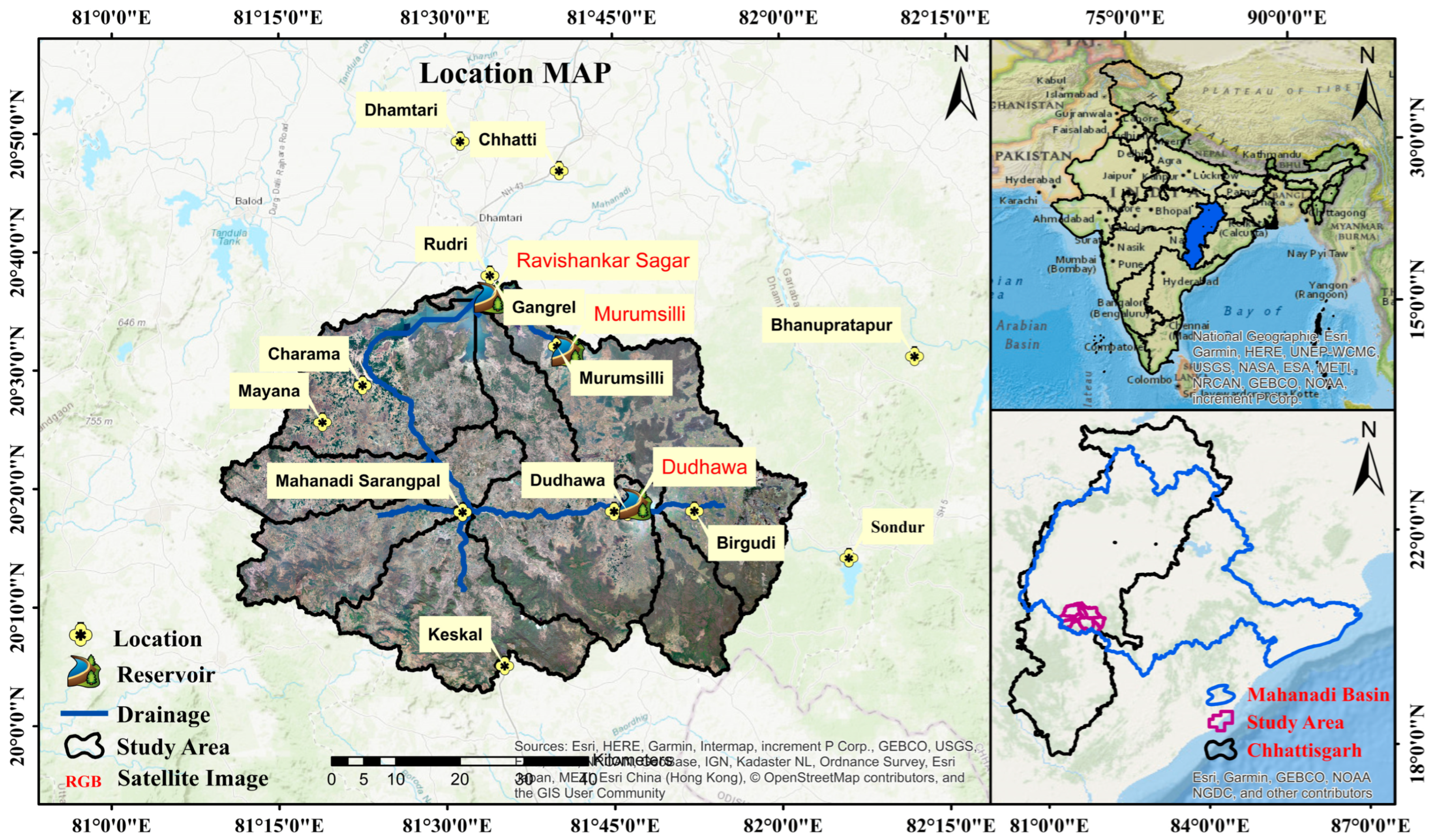
2.1. Study Area and Data Used

The Mahanadi River is an east-flowing river in East Central India [68,69,70,71] and is popular for the Hirakund dam; in Chhattisgarh, the same river is widely recognized for the Mahanadi Reservoir Project (MRP) complex. The MRP complex is located in the Dhamtari district of Chhattisgarh. It consists of three reservoirs, namely Ravishankar Sagar, usually known as Gangrel Dam, Mururmsilli, and Dudhawa. Murumsilli Dam is constructed in the Silyari River basin. Silyari, which is a tributary of the Mahanadi River. The Murumsilli and Dudhawa dams act as feeders for the Gangrel Dam. In Chhattisgarh, there is a well-known reservoir called the “Gangrel Dam” or “Ravishankar Sagar Reservoir”. It is situated along the Mahanadi River, near the city of Dhamtari. Gangrel Dam serves as a crucial water storage facility, providing irrigation and drinking water for the region. The Gangrel Dam is the largest dam among them, having a length of 1830 m and a depth of 30.5 m [72,73,74,75,76]. Additionally, the Gangrel dam is considered an outlet of the MRP complex, which is located at 20°36′37″ N to 81°33′36″ E (see Figure 1). Gangrel Dam is the first multipurpose dam in Chhattisgarh, which supplies water for irrigation and domestic purposes via the Mahanadi feeder canal (MFC) and industrial water supply for the Bhilai steel plant through the Mahanadi main canal (MMC).

Data types and their sources are listed in

Table 2. Input data used in this study.

Data Type	Descriptions	Years/Periods	Sources
Digital elevation model (DEM)	Shutter Radar Topographic Mission (SRTM) of (30 m resolution)	-	(https://www.opentopography.org/ accessed on 10 September 2022)
Land use maps	(30 m resolution)	1985, 1995, 2005 and 2014	Landsat-8 images, USGS Earth Explorer
Soil map	Raster resolution (1:50,000)	-	National Bureau of Soil Survey-Land Use Planning, Nagpur (NBSS-LUP)
Weather data	Daily basis	1985–2020	Indian Meteorological Department, Pune, India
Hydrological data	Monthly discharge at the reservoir site	1985–2020	Mahanadi Reservoir Project complex in Rudri division, Dhamtari, Chhattisgarh

. The daily weather data from 1985–2020 are taken from the Indian Meteorological Department (IMD) in Pune, India (https://www.imdpune.gov.in/ accessed on 20 October 2022).

2.2. Model Setup

SWAT is a physically based semi-distributed open-source model that can quantify the streamflow and other hydrological components such as sediment yield transport, nutrients, pesticides, water quality, and best management practices of watersheds on a daily time scale. It can be employed to assess the effects of various LULC changes over different timeframes, including both real and hypothetical scenarios arising from human activities. The model was run with an extension of the Arc SWAT 2012 user interface. A detailed description of how to prepare the input file for database users can be found in the SWAT user manual (http://swat.tamu.edu/documentation/ accessed on 12 January 2005).

The model obeys the water balance equation:

$${\mathrm{S}\mathrm{W}}_{\mathrm{t}}=\mathrm{S}\mathrm{W}+\sum _{\mathrm{t}=1}^{\mathrm{T}}\left(\mathrm{P}-\mathrm{Q}-\mathrm{E}\mathrm{T}-{\mathrm{P}}_{\mathrm{c}\mathrm{o}\mathrm{r}}-\mathrm{Q}\mathrm{R}\right)$$

(1)

From Equation (1), ${\mathrm{S}\mathrm{W}}_{\mathrm{t}}$—final soil water content (mm), SW—the initial soil water content (mm), P—the amount of rainfall (mm), Q—surface runoff (mm), ET—evapotranspiration (mm), ${\mathrm{P}}_{\mathrm{c}\mathrm{o}\mathrm{r}}$—percolation (mm), and QR—return flow (mm). In the present study, as a means of assessing surface runoff, the SCS curve number is used. Percolation was simulated using the crack flow model and storage routing techniques.

In this work, the basin was divided into 13 sub-basins with a threshold drainage area of 10,000 ha, and then the sub-basin was subdivided into 68 hydrologic response units (HRUs) with unique soil, land use, and slope classes.. Furthermore, the simulation covers a total duration of 36 years, spanning from 1985 to 2020. Specifically, the warm-up phase extends from 1985 to 1988, followed by a calibration period from 1989 to 2010, and finally a validation period from 2011 to 2020.

2.3. Criteria for Model Performance Assessments

Various statistical approaches exist in the literature for conducting and assessing the accuracy of models concerning the correspondence between observed and simulated variables. Model accuracy can be defined as the extent to which there is a correlation between the observed and simulated variables [77]. In the present study, statistical methods such as coefficient of determination (R²) [77,78], and Nash-Sutcliffe efficiency (E_NS) [79] are used to assess the model performance as presented in Equations (2) and (3), respectively.

$${\mathrm{R}}^2=\frac{{\left[\sum _i{(Q}_o-{\overline{Q}}_o\right)-(Q_s-{\overline{Q}}_s)]}^2}{{\left[\sum _i{(Q}_o-{\overline{Q}}_o\right)}^2\sum _i{{(Q}_s-{\overline{Q}}_s)}^2]}$$

(2)

$$\mathrm{N}\mathrm{S}\mathrm{E}=1-\left[\frac{\sum _{i=1}^n{\left(Q_o-Q_s\right)}^2}{{\sum }_{i=1}^n{\left(Q_o-{\overline{Q}}_o\right)}^2}\right]$$

(3)

where $Q_o$ represents the observed variable (discharge), $Q_s$ represents the model-simulated variable, ${\overline{Q}}_o$ represents the mean of the observed discharge, and ${\overline{Q}}_s$ represents the mean of the simulated discharge, respectively.

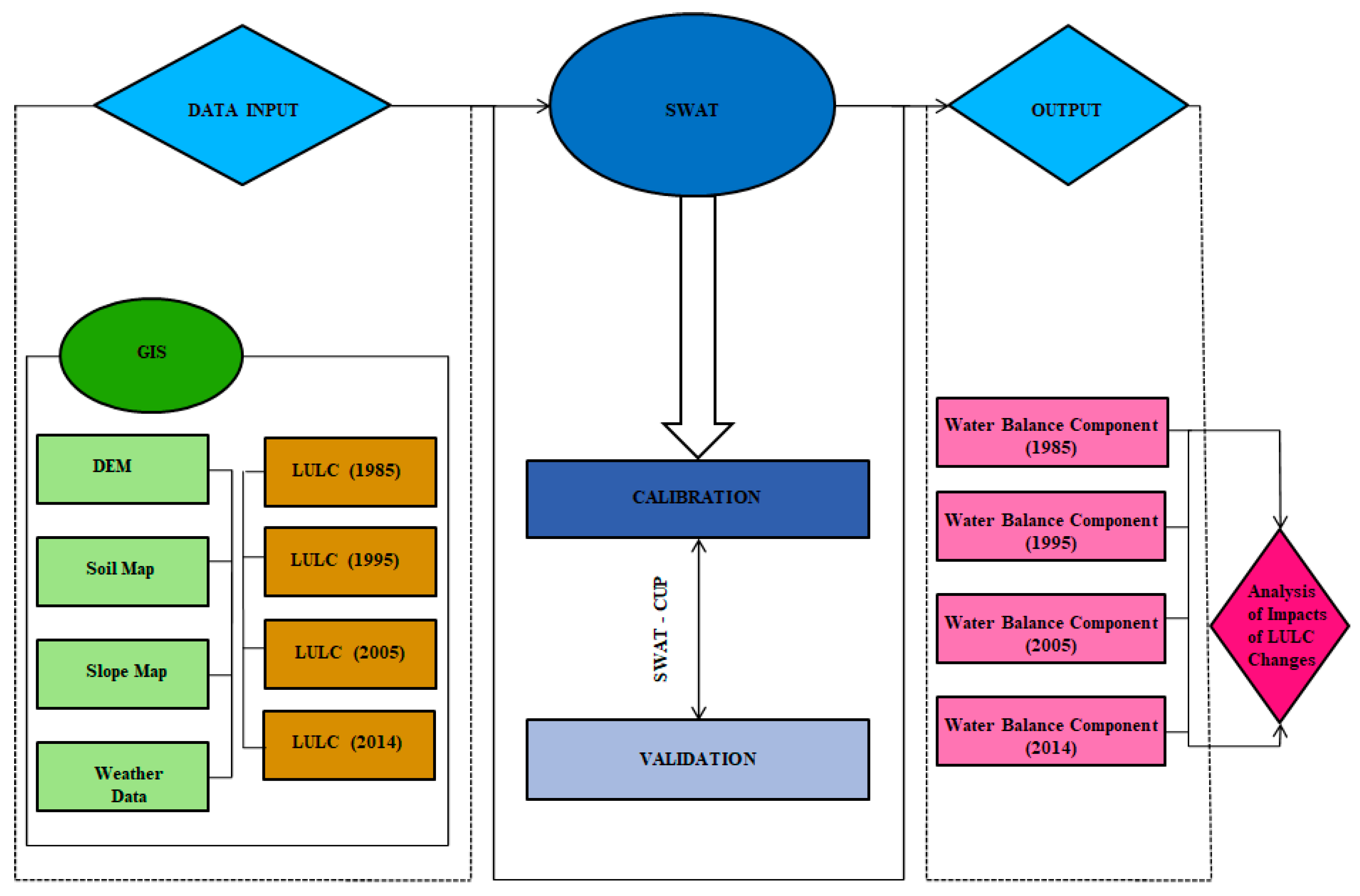
2.4. Overall Methodology

In this section, the methodology adopted for the present study is depicted in Figure 2. However, the entire dataset (i.e., 1985–2020) used in the present study is divided into three different categories: 1985–1996, 1997–2008, and 2009–2020. Land use/land cover maps from the years 1985, 1995, 2005, and 2014 were utilized (refer to Figure 3).

Table 3. List of scenarios used for assessing hydrological impacts during 1985–2020.

Climatic Condition	Scenario Used	Land Use	Duration (Rainfall, Tmax., Tmin.)
C1	S1	1985	1985–1996
	S2	1995	1985–1996
	S3	2005	1985–1996
	S4	2014	1985–1996
C2	S5	1985	1997–2008
	S6	1995	1997–2008
	S7	2005	1997–2008
	S8	2014	1997–2008
C3	S9	1985	2009–2020
	S10	1995	2009–2020
	S11	2005	2009–2020
	S12	2014	2009–2020

presents the twelve scenarios that have been formulated using these various data sources. Understanding the effects of LULC and climate change within the catchment will be much clearer after going through these scenarios.

The terms “real scenario” and “hypothetical scenario” are used to refer to the combination of LULC maps and weather data from the same time and different periods, respectively. When comparing the real and hypothetical scenarios, the combined impacts of LULC and climate can be isolated by assessing the difference in hydrological variables (stream flow, ET, and groundwater flow). Furthermore, in scenarios S1 and S2, the LULC of 1985 and 1995, and weather data of the 1985–1996 period were used, and the term is called real scenario. Furthermore, scenarios S6 and S7 represent actual land use and land cover (LULC) conditions for the years 1995 and 2005, from 1997 to 2008. Similarly, the timeframe of 2009 to 2020, depicted in scenarios S11 and S12, is regarded as a genuine representation of LULC for the years 2005 and 2014, respectively. In hypothetical situations labeled S3 and S4, land use and land cover (LULC) data from 2005 and 2014 were employed, along with weather information spanning the years 1985 to 1996 (refer to Table 3). Furthermore, hypothetical scenarios encompass scenarios S5 and S8, where the land use/land cover (LULC) of 1985 and 2014 during the years 1997–2008 are taken into account. Similarly, the timeframe 2009–2020 (encompassing scenarios S9 and S10) is also treated as a hypothetical scenario for the LULC of 1985 and 1995, respectively. Therefore, the disparities in streamflow evaluation between scenarios S1 and S2 would indicate the distinct influence of land use and land cover changes from 1985 to 2008. In scenario S5, land use patterns from 1985 and weather data from 1997 to 2008 were employed. The disparity in streamflow between S5 and S1 would elucidate the specific impact of climate change during the period 1985–2008. In scenario S6, the analysis incorporated land use data from 1995 and weather data spanning 1997 to 2008. By comparing the stream flow results of S6 with those of S1, the identified disparity would reflect the joint influence of changes in land use and climate during the period from 1997 to 2008 (refer to Table 3).

The mathematical expression of the percentage change of stream flow due to independent LULC, climate change, and combined effects of the same are denoted as Equations (4)–(6) correspondingly [80].

$${∆SR}_{LULC}^{1985–1996}=\left(\frac{S_2-S_1}{S_1}\right)\times 100$$

(4)

$${∆SR}_{Climate}^{1985–1996}=\left(\frac{S_5-S_1}{S_1}\right)\times 100$$

(5)

$${∆SR}_{Combined}^{1985–1996}=\left(\frac{S_6-S_1}{S_1}\right)\times 100$$

(6)

The same approach is applied to evaluate the individual and combined impacts of LULC changes and climate change during different periods, namely 1997–2008 and 2009–2020.

3. Results and Discussion

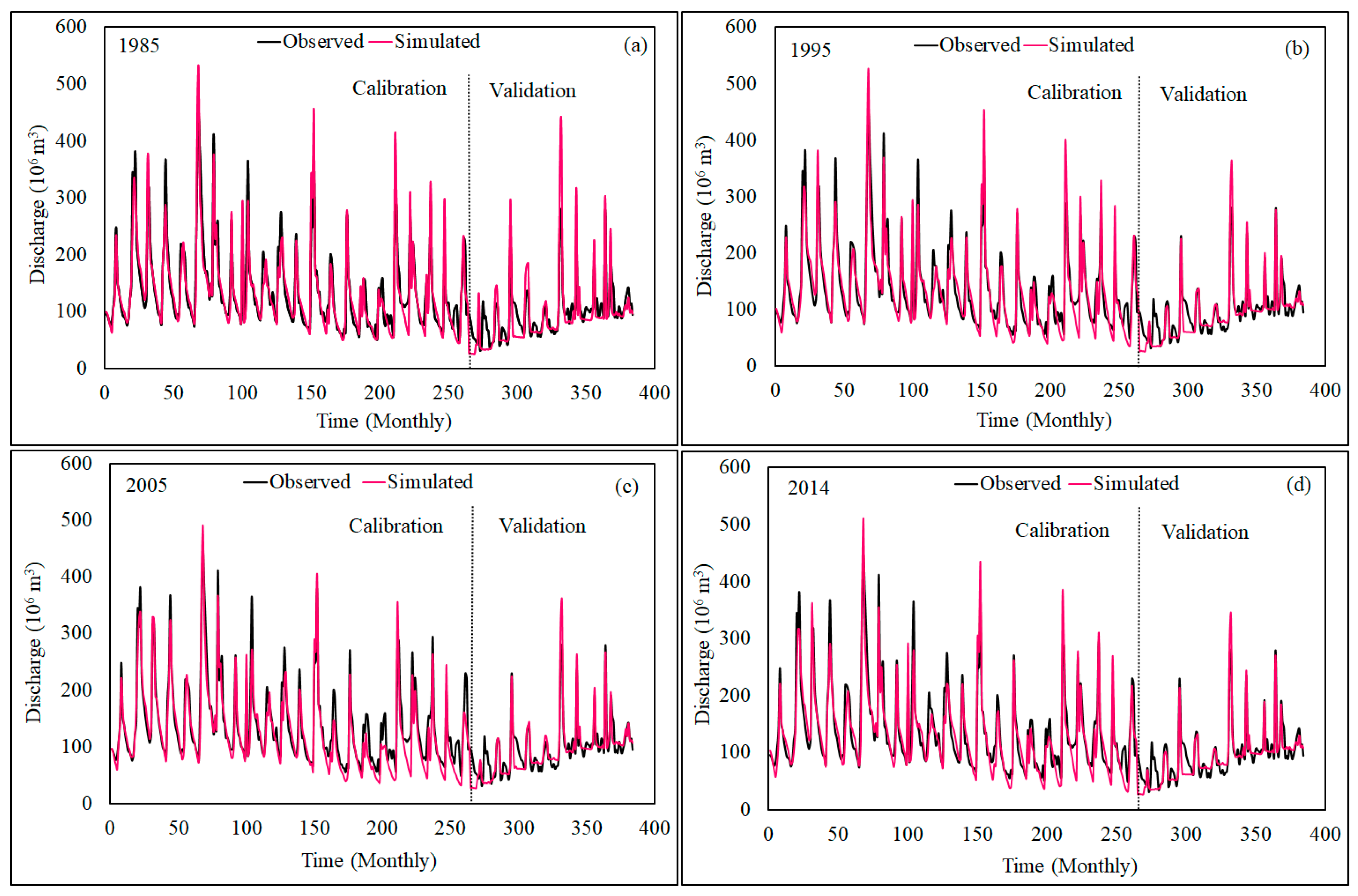
3.1. Model Performance

SWAT was employed to simulate the hydrological processes for the different scenarios using LULC for 1985, 1995, 2005, and 2014 while keeping the other input data constant. The model was then calibrated for the years 1985–2010 with a 4-year warmup period, i.e., 1985–1988. Calibration and validation were performed using SWAT-CUP along with the SUFI-2 algorithm for the 15 selected parameters. In the process of parameterization, certain choices are made concerning the selection of parameters and their initial values for subsequent adjustments. In this particular case, fifteen parameters were carefully chosen, and their initial ranges were established using information obtained from prior research in the relevant field. Both the Relative and Replace approaches were used to adjust the parameters. The Replace option displays the allowable calibration range by showing the minimum and maximum values, while the Relative option indicates modifications made to the original parameters by a specific percentage.

Table 4. List of parameters, accompanied by their respective descriptions, initial minimum and maximum values, as well as the fitted values.

Parameters	Methods	Descriptions	Parameter Range		Fitted Value
			Initial	Final
CN2	Relative	Curve number	−0.30	0.30	0.36
ALPHA_BF	Replace	Base flow alpha factor	0	1	0.56
GW_DELAY	Replace	Groundwater delay	40	480	242.12
GWQMN	Absolute	Shallow aquifer threshold depth of water	0	4500	1.01
GW_REVAP	Replace	Groundwater “Revap” coefficient	0.03	0.3	0.15
ESCO	Replace	Evaporation soil compensation factor	0.02	1	0.90
CH_N2	Replace	Manning’s roughness	0	0.3	−0.08
CH_K2	Replace	Effective hydraulic conductivity	5	130	122.15
ALPHA_BNK	Replace	Base flow alpha factor for bank storage	0	1	0.009
SOL_AWC	Relative	Available water capacity	−0.25	0.25	0.10
SOL_K	Relative	Soil hydraulic conductivity	−0.8	0.8	−0.05
SOL_BD	Relative	The density of soil mass	−0.5	0.7	0.80
HRU_SLP	Relative	Slope steepness	0	0.2	0.06
OV_N	Relative	Overland Manning’s roughness	0.05	35	−0.15
SLSUBBSN	Relative	Slope length	0	0.2	0.02

presents a comprehensive list of parameters, accompanied by their respective descriptions, initial minimum and maximum values, as well as the fitted values obtained after the calibration analysis. The results from the adjusted parameters indicate that out of the 15 parameters, certain parameters (i.e., ALPHA_BANK, CH_K2, SOIL_AWC, CN2, GW_DELAY, and HRU_SLP) exhibited a higher degree of sensitivity (refer to Table 4).

Table 5. Model performance results at the reservoir site.

Statistical Indices		LULC Scenarios
		Criteria for Satisfactory	1985	1995	2005	2014
p-factor	Calibration	>0.7	0.91	0.92	0.88	0.88
	Validation		0.98	1.00	0.86	1.00
r-factor	Calibration	<1.5	1.01	1.00	1.09	1.07
	Validation		1.20	0.85	0.87	0.93
R2	Calibration	>0.5	0.86	0.84	0.88	0.85
	Validation		0.82	0.82	0.82	0.81
NSE	Calibration	>0.5	0.85	0.83	0.85	0.83
	Validation		0.72	0.74	0.74	0.75
RSR	Calibration	≤0.7	0.39	0.42	0.39	0.41
	Validation		0.69	0.52	0.51	0.50
PBIAS	Calibration	<±25	1.90	2.90	8.40	4.30
	Validation		6.10	2.90	1.20	3.80

indicates the results of model performance during the calibration and validation phases of the reservoir outlet. Furthermore, Table 5 illustrates the acceptable and satisfactory performance of the model [79,80,81]. Figure 4 depicts the graphical representation of the optimum simulated flow on the monthly time step compared with the observed data. For calibration (1989–2010) and validation (2011–2020) purposes, the model was run from 1985 to 2020 with different LULCs, respectively (i.e., 1985, 1995, 2005, and 2014). It is evident from Figure 4 that the simulated monthly peak flow values are closely matched with the observed ones. It is observed from Table 5 that the simulated values are evenly distributed during both the calibration and validation phases. Satisfactory values were obtained during the calibration and validation phase with LULC in 2005 (i.e., R² = 0.88, E_NS = 0.85, and R² = 0.82, E_NS = 0.74). Furthermore, comparable outcomes were obtained for the various LULC datasets, specifically for the years 1985, 1995, and 2014, throughout both the calibration and validation phases as per the criteria provided by Moriasi et al. [81] (refer to Table 5). Consequently, the outcomes derived from the model across various LULC scenarios yield a pleasing simulation of monthly discharge within the catchment.

3.2. Influence of LULC Change and Climate Variability on Hydrology under the Real Scenario

This section presents a real scenario aimed at comprehending the hydrology of the Mahanadi Reservoir catchment area. The study focuses on specific combinations: climatic condition (C1) during 1985–1996 paired with land use data from 1985 (S1); climatic condition (C1) during 1985–1996 paired with land use data from 1995 (S2); climatic condition (C2) during 1997–2008 paired with land use data from 1995 (S6); and climatic condition (C2) during 1997–2008 paired with land use data from 2005 (S7). Similarly, the climatic condition (C3) of 2009–2020 was chosen with a land use of 2014 (S12) (refer to Table 3). The findings were condensed to reflect alterations in land use and climatic conditions (S1 compared to S6), leading to a rise in average annual precipitation and evapotranspiration (ET) by 9.1 mm and 589.2 mm, respectively. Additionally, there was a reduction in groundwater recharge (GwQ), low-flow quantity (LQ), and surface runoff (R) by 349.02 mm, 57.35 mm, and 174.02 mm, respectively. Similarly, in scenario S2, analogous alterations are observed as in scenario S7. Precipitation and ET exhibit increments of 9.1 mm and 658.3 mm, while GwQ, LQ, and R display decreases of 327.88 mm, 81.33 mm, and 211.42 mm, respectively. Nevertheless, for scenario S7 with S12 modifications, changes were evident in a distinct manner. Notably, there was a rise of 210.2 mm in ET, while the other water balance parameters exhibited decreases as follows: precipitation by 118.4 mm, GwQ by 143.02 mm, LQ by 6.57 mm, and surface runoff by 162.99 mm, respectively (refer to Figure 5a,b). As a result, when considering the scenario of land use change (S1 with S2) while keeping the climatic conditions constant (1985–1996), the outcomes differ significantly compared to situations where both land use and climatic conditions change. Consequently, the summarized findings indicate that the average annual precipitation amount remains unchanged. However, the other parameters related to water balance experienced reductions: ET decreased by 0.1 mm, GwQ by 2.81 mm, LQ by 0.03 mm, and R by 0.67 mm (refer to Figure 5a). Furthermore, a comparable trend has been noticed in the context of the land use change scenarios (S6 with S7) alongside the climatic conditions from 1985 to 1996. The ensuing outcomes are as follows: there is no alteration in precipitation, while both ET and GwQ exhibit increments of 69 mm and 18.51 mm, respectively. Conversely, LQ and R experience decreases of 24.01 mm and 36.73 mm, respectively (refer to Figure 5b).

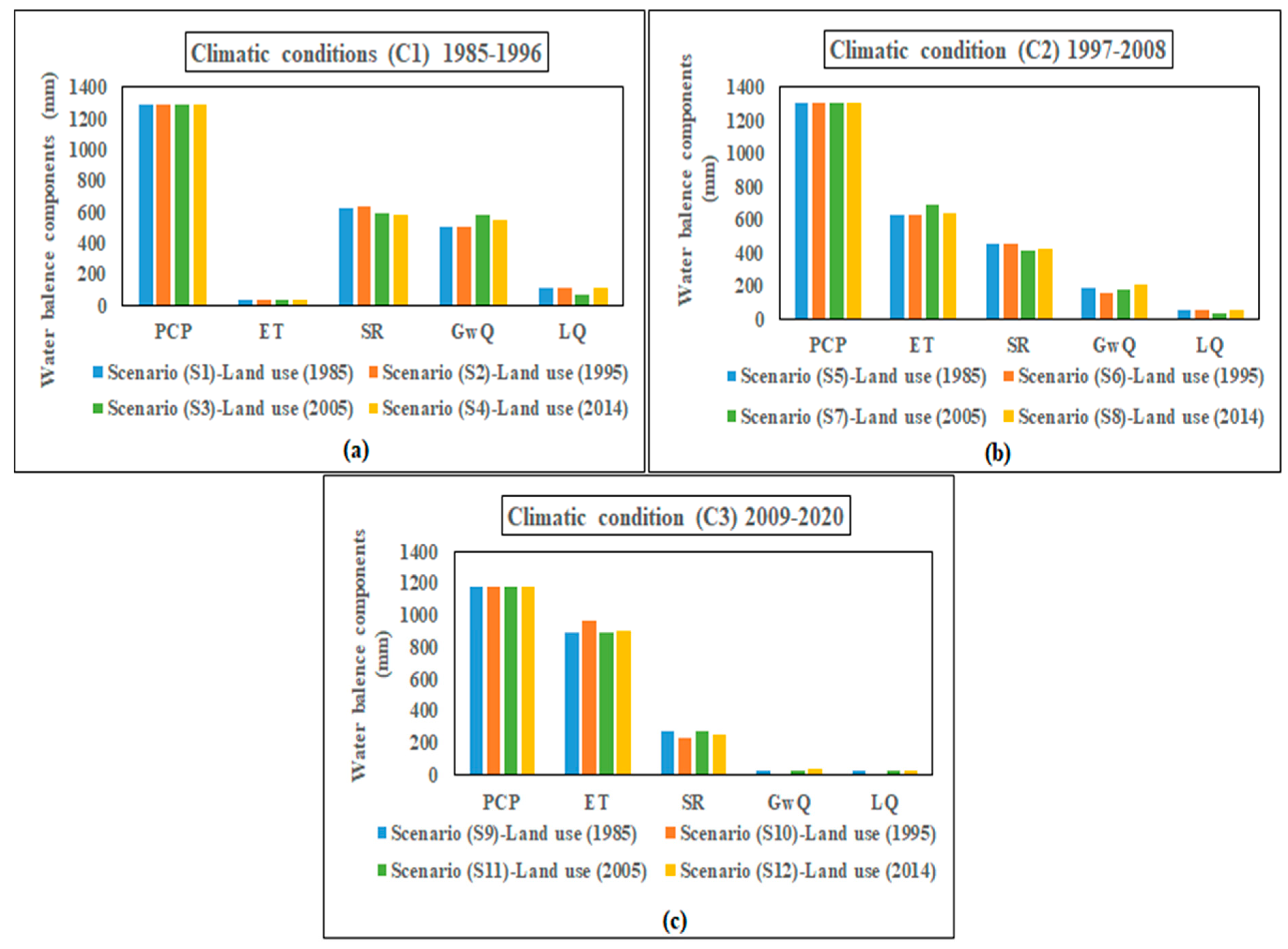
3.3. Influence of LULC Change and Climate Variability on Hydrology under the Hypothetical Scenario

In this section, diverse land uses are contrasted under different climatic conditions to analyze the influence of both land use and climate on hydrology. SWAT simulates precipitation with hydrological components including streamflow, groundwater flow (GwQ), lateral flow (LQ), and evapotranspiration (ET) under varying land use patterns and climatic conditions, as depicted in Figure 5a–c. Table 3 shows the multiple hypothetical scenarios, S1, S2, S3, and S4, along with different land uses, such as 1985, 1995, 2005, and 2014, respectively, with the climatic conditions of 1985–1996 implying the need to understand the effect of land use as well as the climate change scenario. Similarly, Table 3 depicts the hypothetical scenarios S5, S6, S7, and S8 with climatic conditions from 1997–2008 and the hypothetical scenarios S9, S10, S11, and S12 with climatic conditions from 2009–2020 with the combination of different land uses from 1985, 1995, 2005, and 2014, respectively.

When contrasting the scenario depicted in Figure 5a, specifically scenario S1, which pertains to land use in 1985 and the period between 1985 and 1996, with scenarios S2, S3, and S4, the observations revealed variations in surface runoff. In S2, there was an increment of 0.67 mm, whereas in S3 and S4, there were reductions of 39.68 mm and 43.95 mm, respectively, both concerning land use years 1995, 2005, and 2014. Nevertheless, scenario S2 experiences a reduction in GwQ of 2.81 mm, whereas scenarios S3 and S4 encounter rises of 73.95 mm and 41.79 mm, respectively. Similarly, for S1, there was a reduction of 0.1 mm in ET, while for S3 and S4, there was an increase of 0.2 mm each. As a result, for scenarios S2, S3, and S4, there is a reduction of 0.03 mm and 43.84 mm, respectively, and an increase of 1.24 mm in the case of LQ. Furthermore, comparable outcomes can be achieved across various hypothetical situations, each characterized by distinct levels of magnitude (see Figure 5b).

A comparative analysis was conducted using a hypothetical scenario to arrive at a certain conclusion. The analysis involved three distinct scenarios: S1, S5, and S9. In these scenarios, the land use pattern in the year 1985 was contrasted with three different time frames: 1985–1996, 1997–2008, and 2009–2020 (as indicated in Figure 5a, Figure 5b and Figure 5c, respectively). The findings indicate that there is an average annual rise in precipitation of 9.1 mm. This leads to an increase of 589.4 in ET, while GwQ and LQ experience reductions of 322.5 mm and 57.32 mm, respectively, across scenarios S1 to S5. Consequently, there is a decrease of 174.64 mm in streamflow. Conversely, when comparing scenarios S5 to S9, a decrease of 118.44 mm in precipitation results in a decline in streamflow, ET, GwQ, and LQ of 223.15 mm, 265.8 mm, 161.87 mm, and 30.2 mm, respectively. So, the interactions between land use and land cover (LULC) patterns and changes in the weather have a big impact on the hydrology of the Mahanadi Reservoir Project complex and are closely related to each other. This phenomenon is evident in the repeated scenarios denoted as S2, S6, and S10, as well as S3, S7, and S11, along with S4, S8, and S12 (as shown in Figure 5a–c). The findings demonstrate that in the given scenarios (S2 to S6), there is a 9.1 mm rise in precipitation. Additionally, variables such as ET, GwQ, R, and LQ display reductions of 589.3 mm, 346.39 mm, 174.69 mm, and 57.32 mm, respectively. Following that, in the subsequent period (S6 to S10), the results indicate a reduction in precipitation of 118.4 mm. As a result, the remaining water balance parameters also exhibit a decrease (namely, ET of 339.5 mm, GwQ of 151.92 mm, runoff of 223.71 mm, and LQ of 46.76 mm). Moreover, comparable outcomes can be achieved when considering scenarios S3 to S7, as well as the transition from S7 to S11, with varying degrees of impact (as depicted in Figure 5a–c). In the context of scenario S4 with S8, there is an observed increase of 9.1 mm in both precipitation and ET, leading to a corresponding decrease in GwQ, runoff, and LQ of 341.05 mm, 158.36 mm, and 58.28 mm, respectively. Likewise, in the case of S8 combined with S12, there is a reduction of 118.4 mm in precipitation, accompanied by a 270 mm increase in ET. As a result, this leads to a decrease of 174.42 mm, 171.4 mm, and 30.89 mm in GwQ, Runoff, and LQ, respectively, as illustrated in Figure 5a–c.

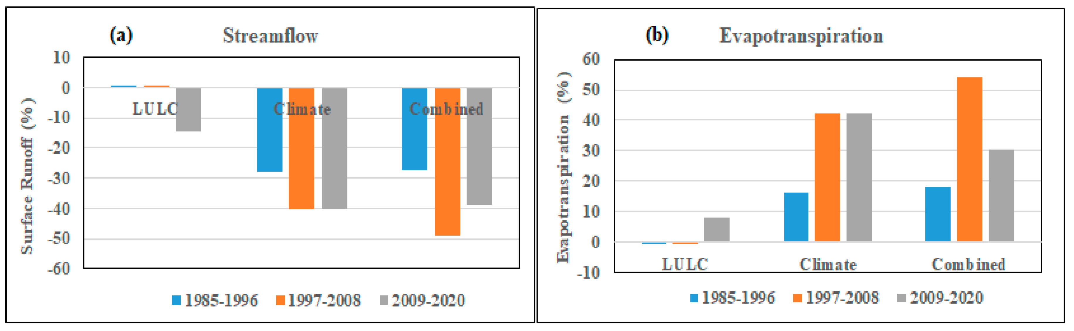
3.4. Isolated Influence of LULC on Streamflow, ET

Figure 6a illustrates that land use and land cover (LULC) changes resulted in a minor rise in streamflow during 1985–1996 and 1997–2008. However, a noteworthy surge of 14.69% in streamflow was recorded from 2009 to 2020, indicating a substantial impact of LULC changes during this period. The period between 2009 and 2020 saw the most significant reduction in streamflow, and during this time, the rate of decrease within the settlement area escalated to 36.36%, as indicated in

Table 6. LULC change detection analysis from 1985–2020.

LULC Classes	Area 1985 (%)	Area 1995 (%)	RoC (%)	Area 1995 (%)	Area 2005 (%)	RoC (%)	Area 2005 (%)	Area 2014 (%)	RoC (%)
FRSD	45.36	43.74	−3.57	43.74	43.20	−1.23	43.20	42.07	−2.61
AGRR	38.95	39.83	2.26	39.83	40.44	1.53	40.44	42.73	5.66
URBN	0.25	0.29	1.00	0.29	0.32	10.34	0.32	0.46	43.75
FRST	3.72	4.11	10.48	4.11	4.14	0.72	4.14	5.01	21.01
RNGB	2.92	3.28	12.32	3.28	3.16	−3.65	3.16	1.80	−43.03
BARR	0.60	0.63	5.00	0.63	0.66	4.76	0.66	0.9	36.36
AGRL	1.06	0.92	−13.20	0.92	0.92	0.00	0.92	4.87	81.07
WATR	3.07	3.08	2.28	3.08	3.10	0.64	3.10	3.67	18.38
FRSE	4.07	4.07	0.00	4.07	4.07	0.00	4.07	6.74	65.60

. Consequently, the expansion of impermeable surfaces due to urbanization primarily results in reduced soil infiltration. This reduction in base flow contributes to heightened surface runoff, culminating in more frequent occurrences of floods [82,83,84,85,86].

The analysis of land use and land cover (LULC) revealed a decrease in evapotranspiration (ET) during the two studied periods, 1985–1996 and 1997–2008. Specifically, there was a reduction of 0.27% and 0.03% in ET for each respective period. This decline in ET raises significant concerns as it directly relates to the decline in vegetation cover, water bodies, and agricultural land. While changes in land use and land cover (LULC) led to an 8.24% increase in evapotranspiration (ET) between 2009 and 2020, during the period from 2005 to 2014, there was an increase of 36.36% in barren land, 18.38% in water bodies, and 65.60% in forest cover. The barren land also experienced an acceleration in the rate of change, rising from 4.76% in 1995 to 5.00% in 2005. Similarly, the rate of change under water bodies increased from 2.28% in 1995 to 0.64% in 2005. Finally, the rate of change within the forest cover remained consistent and subsequently surged by 65.60% in 2014 (see Table 6).

3.5. Isolated Influence of Climate Variability on Streamflow, ET

In Figure 6a, it can be observed that there was a consistent reduction in stream flow throughout the three examined time spans: 1985–1996, 1997–2008, and 2009–2020. The decrease in stream flow was recorded at rates of 27.74%, 40.26%, and 40.25%, respectively. The period from 1997 to 2008 marked a significant reduction in stream flow, primarily attributed to increased evapotranspiration (ET) caused by factors such as the expansion of barren land, water bodies, agricultural activities, and forest cover. The rate of change under barren land, water bodies, agricultural, and forest cover increases by 4.76%, 0.64%, 81.07%, and 65.60%, respectively, as shown in Table 6. Furthermore, the results indicate an increase in ET during all three analyzed periods, i.e., 1985–1996, 1997–2008, and 2009–2020, by 16.19%, 42.47%, and 42.4%, respectively (refer to Figure 6b). Therefore, this results in a decrease in stream flow. The period from 1997 to 2008 exhibited the most significant reduction in ET. This decline can be primarily attributed to the expansion of barren land, water bodies, agricultural activities, and forest cover. Similarly, the rate of change under water bodies, agricultural, and forest cover increased from 2.28%, 2.26%, and 10.48% in 1995 to 0.64%, 1.53%, and 0.72% in 2005. It also further increases from 18.38%, 5.66%, and 21.01% in 2014, respectively, as presented in Table 6.

3.6. The Combined Influence of LULC and Climate Variability on Streamflow, ET

In this particular section, it is evident that there has been a consistent reduction in stream flow throughout the three examined time spans: 1985–1996, 1997–2008, and 2009–2020. The decrease in stream flow amounts to 27.64%, 49.04%, and 38.91% for each respective period, as depicted in Figure 6a. The rate of change within the settlement exhibits a continuous rise, starting at 1.00% in 1995 and progressively climbing to 10.34% in 2005. Moreover, it continues to surge, reaching 43.75% in 2014. Unfortunately, stream flow still decreases during all three analyzed periods due to an increase in ET. Therefore, this results in a decrease in stream flow. As a result, there was a significant increase in ET during all three analyzed periods, i.e., 1985–1996, 1997–2008, and 2009–2020, by 18.18%, 54.21%, and 30.26%, respectively, as shown in Figure 6b. Hence, a decrease in stream flow was observed in all three analyzed periods. The maximum increase in ET was observed for climatic conditions (C2), i.e., 1997–2008, by 54.21%. Therefore, the increase in ET is mainly due to an increase in barren land, water bodies, and agricultural and forest cover.

The runoff-rainfall ratio (RR) and dryness index (ET/P) were computed for three different periods (1985–1996, 1997–2008, and 2009–2020) across various land uses and land cover (LULC). The analysis revealed that changes in both LULC patterns and climatic variations contributed to an increase in RR and a reduction in the dryness index during the initial two periods, considering multiple scenarios of LULC distribution (i.e., 1985, 1995, 2005, and 2014). During the period from 2009 to 2020, there was an observed decline in the RR ratio along with an increase in the dryness index across various LULC scenarios, specifically those representing the years 1985, 1995, 2005, and 2014. This trend is attributed to a combination of LULC changes and climatic variations, as depicted in Figure 7a–d.

Relative to the period between 1985 and 1996, the percentage change under the RR has shown a notable increase of 70% for the years 2009–2020. Concurrently, the dryness index has demonstrated a substantial reduction of 72% during the same time frame. Likewise, when comparing the 1985–1996 period to the subsequent years of 1997–2008, the RR displays a heightened increase of 44%, while the dryness index experiences a decreased value of 45% (refer to Figure 7a).

The land use and land cover (LULC) data from 1995 show a 75% increase in the rate of change under the RR from 2009 to 2020. Concurrently, the dryness index exhibited a 78% decrease when compared to the period of 1985 to 1996. Interestingly, the percentage change in RR and the dryness index observed from 1985–1996 to 1997–2008 mirrored the pattern seen in LULC for the year 1985 (refer to Figure 7b).

In Figure 7c, changes in RR between 2009 and 2020, concerning LULC in 2005, exhibit a 69% increase compared to the changes observed from 1985 to 1996. Moreover, there is a notable 72% reduction in the dryness index. Similarly, Figure 7c shows that from 1985 to 1996 to 1997 to 2008, the RR increased by 47% while the dryness index decreased by 50%.

Regarding the LULC data for the year 2014, there has been a 70% increase in the percentage change under RR between the years 2009 and 2020. Simultaneously, the dryness index has exhibited a 73% decrease during the same period. Likewise, when comparing the periods 1985–1996 and 1997–2008, there has been a 44% rise in RR and a corresponding 46% decrease in the dryness index, as depicted in Figure 7d.

Similar to numerous other Indian watersheds, the Mahanadi Reservoir Project complex faces challenges due to the expanding urban and rural population as well as the impacts of climate calamities. Consequently, the government organization responsible for rehabilitating natural resources needs to formulate management strategies and implement suitable interventions.

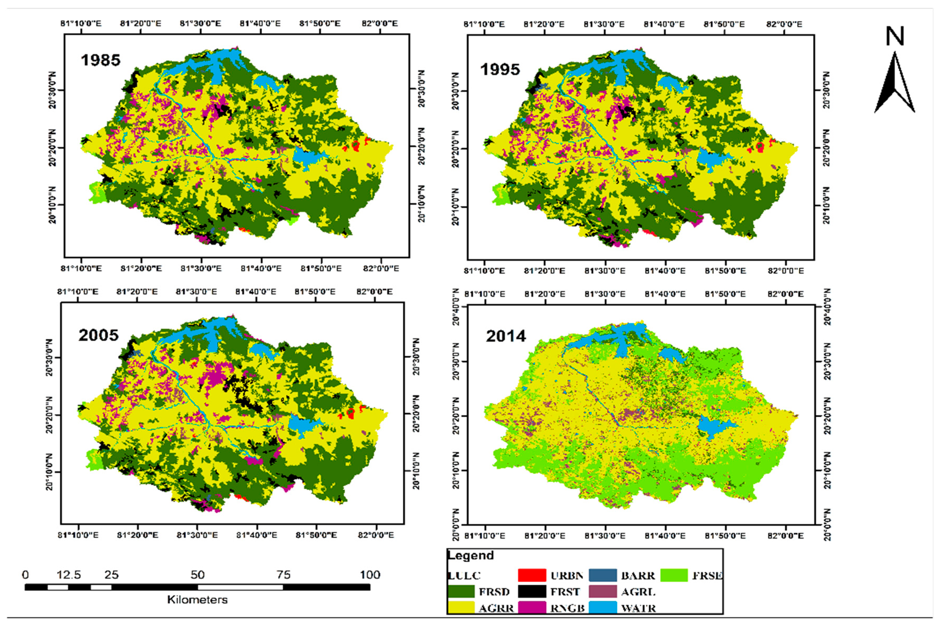
3.7. Influence of Land Use/Land Cover Change Analysis

The main focus of researchers has been on understanding the effects of altering land use on water resources, and an effective technique for this purpose is employing an integrated modeling approach [87,88,89,90,91]. Choi and Deal [92] also employed this approach to enhance the demonstration of how the process of urbanization impacts the hydrological characteristics of a watershed. They subsequently integrated this data with a dynamic model of urban expansion known as LEAMluc. Changes in land use had a significant impact on the hydrological processes of the basin, increasing streamflow and water yield and decreasing infiltration and base flow. Hence, it is possible to combine a distributed hydrological model with land use models to obtain precise data regarding how changes in land use patterns impact the hydrological system’s behavior.

To assess the effects on the hydrological component, the analysis of land use and land cover changes in this study was initiated in 1985, considering alterations in 1985, 1995, 2005, and 2014. The predominant land uses in the vicinity of the Mahanadi Reservoir Project (MRP) encompassed the following categories: deciduous forest (FRSD), row crops (AGRR), residential areas (URBN), mixed forest (FRST), range brush (RNGB), barren land (BARR), agricultural land (AGRL), water bodies (WATR), and evergreen forest (FRSE). These categories collectively accounted for nearly 99% of the land cover, although their proportional distributions varied considerably depending on the specific scenario (refer to Table 6).

The evolution of LULC concerning MRP over different periods is illustrated in Table 6. The rate of change (RoC) in built-up areas exhibited a progression from 1985 to 1995 (1.00%); 1995 to 2005 (10.34%); and 2005 to 2014 (43.75%). These changes reflect the accelerating pace of urbanization and settlement growth observed in recent years, which has led to a relatively minor rise in streamflow due to the concurrent increase in evapotranspiration (ET).

During the analyzed periods (1985–1995, 1995–2005, and 2005–2014), the mixed forest’s RoC increased by 10.48%, 0.72%, and 21.01%, respectively (refer to Table 6). This demonstrates that environmental system changes became much more intense during these decades. As a result, we need to make substantial progress towards greater drought resilience, water availability, water uptake, and water use efficiency. Whereas, in the deciduous forest, the RoC decreased by −3.57% between 1985–1995, −1.23% between 1995–2005, and −2.61% between 2005–2014. Consequently, significant changes occurred within the environmental system over these decades. This led to the clearing of forests for various activities, like agriculture and construction. The proportion of land dedicated to agricultural row crops saw a notable rise from 2.26% during 1985–1996 to 1.53% between 1997–2008, and further to 5.66% spanning 2009–2020. Moreover, the reduction of deciduous forests increases the planet’s vulnerability to the impacts of global warming, resulting in significant changes to the climate.

The studied periods (1985–1995, 1995–2005, and 2005–2014) show respective rises in the rate of change of barren land of 5.00%, 4.76%, and 36.36%, as indicated in Table 6. As a result, the expansion of wastelands is directly linked to the rise in evapotranspiration, subsequently leading to a reduction in streamflow. Likewise, the RoC beneath water bodies exhibited a rise of 2.28% during 1985–1995, followed by increments of 0.64% and 18.38% in the periods 1995–2005 and 2005–2014, as indicated in Table 6. Therefore, the increase in ET can be directly attributed to the extent of the water bodies. As a result, the streamflow is diminished.

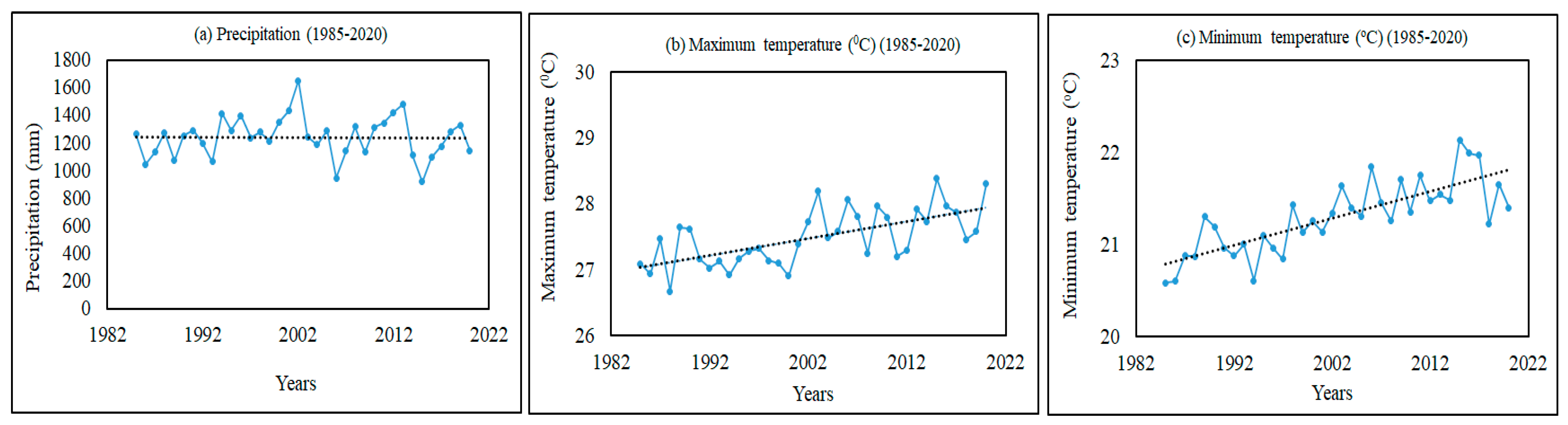
3.8. Variability and Trend of Precipitation and Temperature Variables

Figure 8a–c shows the graphical representation of time (in years) with respect to meteorological variables (i.e., precipitation, Tmax, and Tmin). According to Figure 8a, precipitation variables are constant throughout time. In the present analysis, we have taken the mean of all the stations mentioned in the study area section and then examined the trend of precipitation for the entire study area. Similarly, for maximum and minimum temperatures, we determine the overall temperature for the entire study area and examine the trends for the same. As per Figure 8b, the maximum temperature continuously increases in an upward direction over time (1985–2020); similarly, the minimum temperature significantly increases over time (refer to Figure 8c). Therefore, there is no noteworthy trend in the precipitation patterns of the study area, but there has been a consistent upward trend in both the maximum and minimum temperatures. This indicates a shifting climate pattern characterized by escalating temperatures, which could have diverse effects on the environment. To gain a better grasp of the reasons behind these temperature fluctuations and their potential consequences on the area’s ecosystems, water reserves, and human undertakings, additional in-depth investigation is required. It is imperative to closely observe and adjust to these changes to make well-informed choices and ensure the responsible stewardship of the region’s resources and infrastructure.

4. Conclusions

Land use land cover (LULC), and climate are still changing due to anthropogenic and other atmospheric factors. These two factors are significantly responsible for changing watershed hydrology across the globe. This study aims to evaluate the impact of LULC on the hydrological processes of the Mahanadi Reservoir Project (MRP) in Chhattisgarh, India. The Soil and Water Assessment Tool (SWAT) was used to simulate the different hydrological components and impacts of LULC on the same. Twelve scenarios were considered using 1985–1996, 1997–2008, and 2009–2020 and four sets of land use maps. The Mahanadi Reservoir complex exhibits a decrease in streamflow and an increase in evapotranspiration (ET) owing to the increased water bodies, vegetation cover, and barren land. Subsequently, streamflow and ET show a similar trend, despite a different magnitude, when considering climate variability, and the combined effects of land use and climate variability on streamflow and ET show an inverse relationship.

This research utilized a semi-distributed SWAT model to examine the effects of LULC and climate change on the catchment of the Mahanadi Reservoir complex. The findings demonstrate that the utilization of the SWAT model offers an efficient approach to evaluating the Mahanadi Reservoir complex, enabling its potential application in forthcoming research endeavors. The Mahanadi Reservoir complex experiences a reduction in stream flow and a rise in evapotranspiration due to the combined influence of expanding water bodies, forest cover, and increased barren land. When examining the individual impact of climate change, both streamflow and evapotranspiration demonstrate a similar trend, although at varying levels of intensity. Furthermore, there is an inverse relationship between land use and climatic variability in the Mahanadi Reservoir complex catchment, as assessed by the combined effects of both LULC and climate change on streamflow and ET. Furthermore, this study also employed the SWAT model to assess the impact of land use and land cover changes on the various components of the water balance. Between 1985 and 2014, the LULC within the MRP catchment area experienced notable changes. The proportions of mixed forest increased from 3.72% to 5.01%, urbanization increased from 0.25% to 0.46%, deciduous forest declined from 45.36% to 42.07%, agricultural row crops saw an increase from 38.95% to 42.73%, shrubland decreased from 2.92% to 1.80%, barren land expanded from 0.60% to 0.90%, agricultural areas expanded from 1.06% to 4.87%, evergreen forest expanded from 4.07% to 6.74%, and water bodies increased from 3.07% to 3.67%. These changes denote significant alterations in the landscape over this period.

The outcomes of the SWAT simulation demonstrate the significant impacts of LULC changes on hydrological processes. Under climate scenario C1, the mean annual stream flow exhibited a decline from 629.62 mm to 585.67 mm between 1985 and 2014. Meanwhile, for the same timeframe and under climate scenario C3, the stream flow decreased from 271.83 mm to 255.88 mm. The average annual ET exhibited distinct trends, ranging between 36.4 and 36.5 mm from 1985 to 2014 under climate conditions (C1) and between 891.6 and 904.8 mm under climate conditions (C3). Consequently, the study determined that changes in LULC would significantly impact these hydrological processes. Thus, the augmentation of barren land, expansion of forest cover, and increase in water body areas all play a significant role in amplifying ET quantities within the MRP complex.

References

1. Cook, J.; Oreskes, N.; Doran, P.T.; Anderegg, W.R.L.; Verheggen, B.; Maibach, E.W.; Carlton, J.S.; Lewandowsky, S.; Skuce, A.G.; A Green, S.; et al. Consensus on consensus: A synthesis of consensus estimates on human-caused global warming. Environ. Res. Lett. 2016, 11, 048002. [Google Scholar] [CrossRef]
2. Jiménez-Navarro, I.C.; Jimeno-Sáez, P.; López-Ballesteros, A.; Pérez-Sánchez, J.; Senent-Aparicio, J. Impact of Climate Change on the Hydrology of the Forested Watershed That Drains to Lake Erken in Sweden: An Analysis Using SWAT+ and CMIP6 Scenarios. Forests 2021, 12, 1803. [Google Scholar] [CrossRef]
3. Kiesel, J.; Gericke, A.; Rathjens, H.; Wetzig, A.; Kakouei, K.; Jähnig, S.C.; Fohrer, N. Climate change impacts on ecologically relevant hydrological indicators in three catchments in three European ecoregions. Ecol. Eng. 2019, 127, 404–416. [Google Scholar] [CrossRef]
4. Wu, J.; Yen, H.; Arnold, J.G.; Yang, Y.E.; Cai, X.; White, M.J.; Santhi, C.; Miao, C.; Srinivasan, R. Development of reservoir operation functions in SWAT+ for national environmental assessments. J. Hydrol. 2020, 583, 124556. [Google Scholar] [CrossRef]
5. Cerdà, A.; Ackermann, O.; Terol, E.; Rodrigo-Comino, J. Impact of Farmland Abandonment on Water Resources and Soil Conservation in Citrus Plantations in Eastern Spain. Water 2019, 11, 824. [Google Scholar] [CrossRef]
6. Cerdà, A.; Rodrigo-Comino, J.; Yakupoğlu, T.; Dindaroğlu, T.; Terol, E.; Mora-Navarro, G.; Arabameri, A.; Radziemska, M.; Novara, A.; Kavian, A.; et al. Tillage Versus No-Tillage. Soil Properties and Hydrology in an Organic Persimmon Farm in Eastern Iberian Peninsula. Water 2020, 12, 1539. [Google Scholar] [CrossRef]
7. Zierl, B.; Bugmann, H. Global change impacts on hydrological processes in Alpine catchments. Water Resour. Res. 2005, 41, 1–13. [Google Scholar] [CrossRef]
8. Hagg, W.; Braun, L.; Kuhn, M.; Nesgaard, T. Modelling of hydrological response to climate change in glacierized Central Asian catchments. J. Hydrol. 2007, 332, 40–53. [Google Scholar] [CrossRef]
9. Merritt, W.S.; Alila, Y.; Barton, M.; Taylor, B.; Cohen, S.; Neilsen, D. Hydrologic response to scenarios of climate change in sub watersheds of the Okanagan basin, British Columbia. J. Hydrol. 2006, 326, 79–108. [Google Scholar] [CrossRef]
10. Tan, X.; Liu, S.; Tian, Y.; Zhou, Z.; Wang, Y.; Jiang, J.; Shi, H. Impacts of Climate Change and Land Use/Cover Change on Regional Hydrological Processes: Case of the Guangdong-Hong Kong-Macao Greater Bay Area. Front. Environ. Sci. 2022, 9, 688. [Google Scholar] [CrossRef]
11. Kiros, G.; Shetty, A.; Nandagiri, L. Performance Evaluation of SWAT Model for Land Use and Land Cover Changes under different Climatic Conditions: A Review. J. Waste Water Treat. Anal. 2015, 6, 7. [Google Scholar] [CrossRef]
12. Deng, Z.; Zhang, X.; Li, D.; Pan, G. Simulation of land use/land cover change and its effects on the hydrological characteristics of the upper reaches of the Hanjiang Basin. Environ. Earth Sci. 2015, 73, 1119–1132. [Google Scholar] [CrossRef]
13. Singh, S.K.; Laari, P.B.; Mustak, S.; Srivastava, P.K.; Szabó, S. Modelling of land use land cover change using earth observation data-sets of Tons River Basin, Madhya Pradesh, India. Geocarto Int. 2018, 33, 1202–1222. [Google Scholar] [CrossRef]
14. Kumar, N.; Singh, S.K.; Singh, V.G.; Dzwairo, B. Investigation of impacts of land use/land cover change on water availability of Tons River Basin, Madhya Pradesh, India. Model. Earth Syst. Environ. 2018, 4, 295–310. [Google Scholar] [CrossRef]
15. Gyamfi, C.; Ndambuki, J.M.; Salim, R.W. Hydrological Responses to Land Use/Cover Changes in the Olifants Basin, South Africa. Water 2016, 8, 588. [Google Scholar] [CrossRef]
16. Keesstra, S.; Nunes, J.P.; Saco, P.; Parsons, T.; Poeppl, R.; Masselink, R.; Cerdà, A. The way forward: Can connectivity be useful to design better measuring and modelling schemes for water and sediment dynamics? Sci. Total. Environ. 2018, 644, 1557–1572. [Google Scholar] [CrossRef]
17. Yuan, Z.; Chu, Y.; Shen, Y. Simulation of surface runoff and sediment yield under different land-use in a Taihang Mountains watershed, North China. Soil Tillage Res. 2015, 153, 7–19. [Google Scholar] [CrossRef]
18. Kumar, V.; Kedam, N.; Sharma, K.V.; Mehta, D.J.; Caloiero, T. Advanced Machine Learning Techniques to Improve Hydrological Prediction: A Comparative Analysis of Streamflow Prediction Models. Water 2023, 15, 2572. [Google Scholar] [CrossRef]
19. Mehta, D.; Hadvani, J.; Kanthariya, D.; Sonawala, P. Effect of land use land cover change on runoff characteristics using curve number: A GIS and remote sensing approach. Int. J. Hydrol. Sci. Technol. 2023, 16, 1–16. [Google Scholar] [CrossRef]
20. Calder, I.R. Assessing the water use of short vegetation and forests: Development of the Hydrological Land Use Change (HYLUC) model. Water Resour. Res. 2003, 39, 1318. [Google Scholar] [CrossRef]
21. Amirhossien, F.; Alireza, F.; Kazem, J.; Mohammadbagher, S. A Comparison of ANN and HSPF Models for Runoff Simulation in Balkhichai River Watershed, Iran. Am. J. Clim. Chang. 2015, 04, 203–216. Available online: http://www.scirp.org/journal/PaperInformation.aspx?PaperID=56390&#abstract (accessed on 18 April 2015). [CrossRef]
22. Pfannerstill, M.; Guse, B.; Fohrer, N. Smart low flow signature metrics for an improved overall performance evaluation of hydrological models. J. Hydrol. 2014, 510, 447–458. [Google Scholar] [CrossRef]
23. Madsen, H. Automatic calibration of a conceptual rainfall–runoff model using multiple objectives. J. Hydrol. 2000, 235, 276–288. [Google Scholar] [CrossRef]
24. Shaikh, M.M.; Lodha, P.; Lalwani, P.; Mehta, D. 2022 Climatic projections of Western India using global and regional climate models. Water Pract. Technol. 2022, 17, 1818–1825. [Google Scholar] [CrossRef]
25. Mehta, D.J.; Yadav, S.M. Long-term trend analysis of climate variables for arid and semi-arid regions of an Indian State Rajasthan. Int. J. Hydrol. Sci. Technol. 2022, 13, 191–214. [Google Scholar] [CrossRef]
26. Jimeno-Sáez, P.; Senent-Aparicio, J.; Pérez-Sánchez, J.; Pulido-Velazquez, D. A Comparison of SWAT and ANN Models for Daily Runoff Simulation in Different Climatic Zones of Peninsular Spain. Water 2018, 10, 192. [Google Scholar] [CrossRef]
27. Noori, N.; Kalin, L. Coupling SWAT and ANN models for enhanced daily streamflow prediction. J. Hydrol. 2016, 533, 141–151. [Google Scholar] [CrossRef]
28. Lin, B.; Chen, X.; Yao, H.; Chen, Y.; Liu, M.; Gao, L.; James, A. Analyses of landuse change impacts on catchment runoff using different time indicators based on SWAT model. Ecol. Indic. 2015, 58, 55–63. [Google Scholar] [CrossRef]
29. Farley, K.A.; Jobbagy, E.G.; Jackson, R.B. Effects of afforestation on water yield: A global synthesis with implications for policy. Glob. Chang. Biol. 2005, 11, 1565–1576. [Google Scholar] [CrossRef]
30. Makwana, J.J.; Tiwari, M.K. Hydrological stream flow modelling using soil and water assessment tool (SWAT) and neural networks (NNs) for the Limkheda watershed, Gujarat, India. Model. Earth Syst. Environ. 2017, 3, 635–645. [Google Scholar] [CrossRef]
31. Arnold, J.G.; Srinivasan, R.; Muttiah, R.S.; Williams, J.R. Large area hydrologic modeling and assessment part I: Model development 1. JAWRA J. Am. Water Resour. Assoc. 1998, 34, 73–89. [Google Scholar] [CrossRef]
32. Costa, R.C.A.; Santos, R.M.B.; Fernandes, L.F.S.; de Melo, M.C.; Valera, C.A.; Junior, R.F.D.V.; Silva, M.M.A.P.d.M.; Pacheco, F.A.L.; Pissarra, T.C.T. Hydrologic Response to Land Use and Land Cover Change Scenarios: An Example from the Paraopeba River Basin Based on the SWAT Model. Water 2023, 15, 1451. [Google Scholar] [CrossRef]
33. Marmontel, C.V.F.; Pissarra, T.C.T.; Ranzini, M.; Rodrigues, V.A. Applicability of the SWAT hydrological model in Paraibuna river basin, SP-Brazil. Irriga 2019, 24, 594–609. [Google Scholar] [CrossRef]
34. Sheshukov, A.Y.; Douglas-Mankin, K.R.; Sinnathamby, S.; Daggupati, P. Pasture BMP effectiveness using an HRU-based subarea approach in SWAT. J. Environ. Manag. 2016, 166, 276–284. [Google Scholar] [CrossRef] [PubMed]
35. Grusson, Y.; Anctil, F.; Sauvage, S.; Pérez, J.M.S. Testing the SWAT Model with Gridded Weather Data of Different Spatial Resolutions. Water 2017, 9, 54. [Google Scholar] [CrossRef]
36. DeFries, R.; Eshleman, K.N. Land-use change and hydrologic processes: A major focus for the future. Hydrol. Process. 2004, 18, 2183–2186. [Google Scholar] [CrossRef]
37. Kumar, M.; Denis, D.M.; Kundu, A.; Joshi, N.; Suryavanshi, S. Understanding land use/land cover and climate change impacts on hydrological components of Usri watershed, India. Appl. Water Sci. 2022, 12, 39. [Google Scholar] [CrossRef]
38. Sulamo, M.A.; Kassa, A.K.; Roba, N.T. Evaluation of the impacts of land use/cover changes on water balance of Bilate watershed, Rift valley basin, Ethiopia. Water Pract. Technol. 2021, 16, 1108–1127. [Google Scholar] [CrossRef]
39. Saddique, N.; Mahmood, T.; Bernhofer, C. Quantifying the impacts of land use/land cover change on the water balance in the afforested River Basin, Pakistan. Environ. Earth Sci. 2020, 79, 448. [Google Scholar] [CrossRef]
40. Munoth, P.; Goyal, R. Impacts of land use land cover change on runoff and sediment yield of Upper Tapi River Sub-Basin, India. Int. J. River Basin Manag. 2020, 18, 177–189. [Google Scholar] [CrossRef]
41. Kumar, N.; Tischbein, B.; Kusche, J.; Beg, M.K.; Bogardi, J.J. Impact of land-use change on the water resources of the Upper Kharun Catchment, Chhattisgarh, India. Reg. Environ. Chang. 2017, 17, 2373–2385. [Google Scholar] [CrossRef]
42. Takalaa, W.; Tamamc, D. The effects of land use land cover change on hydrological process of Gilgel Gibe, Omo Gibe Basin, Ethiopia. Int. J. Sci. Eng. Res. 2016, 7, 2020. [Google Scholar]
43. Vilaysane, B.; Takara, K.; Luo, P.; Akkharath, I.; Duan, W. Hydrological Stream Flow Modelling for Calibration and Uncertainty Analysis Using SWAT Model in the Xedone River Basin, Lao PDR. Procedia Environ. Sci. 2015, 28, 380–390. [Google Scholar] [CrossRef]
44. Murty, P.S.; Pandey, A.; Suryavanshi, S. Application of semi-distributed hydrological model for basin level water balance of the Ken basin of Central India. Hydrol. Process. 2014, 28, 4119–4129. [Google Scholar] [CrossRef]
45. Yan, B.; Fang, N.; Zhang, P.; Shi, Z. Impacts of land use change on watershed streamflow and sediment yield: An assessment using hydrologic modelling and partial least squares regression. J. Hydrol. 2013, 484, 26–37. [Google Scholar] [CrossRef]
46. Singh, A.; Imtiyaz, M. Application of a Process Based Hydrological Model for Simulating Stream Flow in an Agricultural Watershed of India. In Proceedings of the India Water Week 2012, New Delhi, India, 10–14 April 2012. [Google Scholar]
47. Srinivasan, R.; Zhang, X.; Arnold, J. SWAT ungauged: Hydrological budget and crop yield predictions in the Upper Mississippi River Basin. Trans. ASABE 2010, 53, 1533–1546. [Google Scholar] [CrossRef]
48. Gosain, A.K.; Rao, S.; Basuray, D. Climate Change Impact Assessment on Hydrology of Indian River Basins. Curr. Sci. 2006, 90, 346–353. Available online: http://www.jstor.org/stable/24091868 (accessed on 24 August 2023).
49. Paul, M. Impacts of land use and climate changes on hydrological processes in South Dakota Watersheds. Electron. Theses Diss. 2016, 1018. Available online: https://openprairie.sdstate.edu/etd/1018 (accessed on 24 August 2023).
50. Chen, J.; Chang, H. Relative impacts of climate change and land cover change on streamflow using SWAT in the Clackamas River Watershed, USA. J. Water Clim. Chang. 2020, 12, 1454–1470. [Google Scholar] [CrossRef]
51. Naz, R.; Ashraf, A.; Van der Tol, C.; Aziz, F. Modeling hydrological response to land use/cover change: Case study of Chirah Watershed (Soan River), Pakistan. Arab. J. Geosci. 2020, 13, 1220. [Google Scholar] [CrossRef]
52. Fulaji, B.S. Study of Streamflow Response to Land use Land cover Change in the Nethravathi River Basin, India. Ph.D. Thesis, National Institute of Technology Karnataka, Surathkal, India, 15 November 2015. Available online: https://idr.l1.nitk.ac.in/jspui/handle/123456789/14239 (accessed on 24 August 2023).
53. Kumar, M.; Mahato, L.L.; Suryavanshi, S.; Singh, S.K.; Kundu, A.; Dutta, D.; Lal, D. Future prediction of water balance using SWAT and CA-Markov methods under recent climate projections: A case study of the Silwani watershed (Jharkhand), India. Environ. Sci. Pollut. Res. 2022, preprint. [Google Scholar] [CrossRef]
54. Hengade, N.; I Eldho, T. Assessment of LULC and climate change on the hydrology of Ashti Catchment, India using VIC model. J. Earth Syst. Sci. 2016, 125, 1623–1634. [Google Scholar] [CrossRef]
55. Dadhwal, V.K.; Aggarwal, S.P.; Mishra, N. Hydrological Simulation of Mahanadi River basin and Impact of Land Use/Land Cover Change on Surface Runoff Using a Macro Scale Hydrological Model. In Proceedings of the ISPRS TC VII Symposium –100 Years ISPRS, Vienna, Austria, 5–7 July 2010. [Google Scholar]
56. Zhang, L.; Nan, Z.; Yu, W.; Ge, Y. Modeling Land-Use and Land-Cover Change and Hydrological Responses under Consistent Climate Change Scenarios in the Heihe River Basin, China. Water Resour. Manag. 2015, 29, 4701–4717. [Google Scholar] [CrossRef]
57. Meenu, R.; Rehana, S.; Mujumdar, P.P. Assessment of hydrologic impacts of climate change in Tunga-Bhadra river basin, India with HEC-HMS and SDSM. Hydrol. Process. 2013, 27, 1572–1589. [Google Scholar] [CrossRef]
58. Chen, H.; Tong, S.T.; Yang, H.; Yang, Y.J. Simulating the hydrologic impacts of land-cover and climate changes in a semi-arid watershed. Hydrol. Sci. J. 2015, 60, 1739–1758. [Google Scholar] [CrossRef]
59. Belay, T.; Mengistu, D.A. Impacts of land use/land cover and climate changes on soil erosion in Muga watershed, Upper Blue Nile basin (Abay), Ethiopia. Ecol. Process. 2021, 10, 68. [Google Scholar] [CrossRef]
60. Dwarakish, G.; Ganasri, B. Impact of land use change on hydrological systems: A review of current modeling approaches. Cogent Geosci. 2015, 1, 1115691. [Google Scholar] [CrossRef]
61. Eini, M.R.; Javadi, S.; Shahdany, M.H.; Kisi, O. Comprehensive assessment and scenario simulation for the future of the hydrological processes in Dez river basin, Iran. Water Supply 2021, 21, 1157–1176. [Google Scholar] [CrossRef]
62. Li, H.; Yu, C.; Qin, B.; Li, Y.; Jin, J.; Luo, L.; Wu, Z.; Shi, K.; Zhu, G. Modeling the Effects of Climate Change and Land Use/Land Cover Change on Sediment Yield in a Large Reservoir Basin in the East Asian Monsoonal Region. Water 2022, 14, 2346. [Google Scholar] [CrossRef]
63. Preetha, P.; Hasan, M. Scrutinizing the Hydrological Responses of Chennai, India Using Coupled SWAT-FEM Model under Land Use Land Cover and Climate Change Scenarios. Land 2023, 12, 938. [Google Scholar] [CrossRef]
64. Setyorini, A.; Khare, D.; Pingale, S.M. Simulating the impact of land use/land cover change and climate variability on watershed hydrology in the Upper Brantas basin, Indonesia. Appl. Geomat. 2017, 9, 191–204. [Google Scholar] [CrossRef]
65. Pandey, B.K.; Khare, D.; Kawasaki, A.; Meshesha, T.W. Integrated approach to simulate hydrological responses to land use dynamics and climate change scenarios employing scoring method in upper Narmada basin, India. J. Hydrol. 2021, 598, 126429. [Google Scholar] [CrossRef]
66. Mensah, J.K.; Ofosu, E.A.; Yidana, S.M.; Akpoti, K.; Kabo-Bah, A.T. Integrated modeling of hydrological processes and groundwater recharge based on land use land cover, and climate changes: A systematic review. Environ. Adv. 2022, 8, 100224. [Google Scholar] [CrossRef]
67. Wu, F.; Zhan, J.; Su, H.; Yan, H.; Ma, E. Scenario-Based Impact Assessment of Land Use/Cover and Climate Changes on Watershed Hydrology in Heihe River Basin of Northwest China. Adv. Meteorol. 2015, 2015, 410198. [Google Scholar] [CrossRef]
68. Sahu, R.T.; Verma, M.K.; Ahmad, I. Impact of long-distance interaction indicator (monsoon indices) on spatio-temporal variability of precipitation over the Mahanadi River basin. Water Resour. Res. 2023, 59, e2022WR033805. [Google Scholar] [CrossRef]
69. Sahu, R.T.; Verma, S.; Kumar, K.; Verma, M.K.; Ahmad, I. Testing some grouping methods to achieve a low error quantile estimate for high resolution (0.25° × 0.25°) precipitation data. J. Phys. Conf. Ser. 2022, 2273, 012017. [Google Scholar] [CrossRef]
70. Sahu, R.T.; Verma, M.K.; Ahmad, I. Characterization of precipitation in the subdivisions of the Mahanadi River basin, India. Acta Sci. Agric. 2021, 5, 50–61. [Google Scholar] [CrossRef]
71. Sahu, R.T.; Verma, M.K.; Ahmad, I. Some non-uniformity patterns spread over the lower Mahanadi River Basin, India. Geocarto Int. 2021, 37, 8792–8814. [Google Scholar] [CrossRef]
72. Verma, S.; Sahu, R.T.; Prasad, A.D.; Verma, M.K. Development of an optimal operating policy of multi-reservoir systems in Mahanadi Reservoir Project Complex, Chhattisgarh. J. Phys. Conf. Ser. 2022, 2273, 012020. [Google Scholar] [CrossRef]
73. Verma, S.; Verma, M.K.; Prasad, A.D.; Mehta, D.J.; Islam, M.N. Modeling of uncertainty in the estimation of hydrograph components in conjunction with the SUFI-2 optimization algorithm by using multiple objective functions. Model. Earth Syst. Environ. 2023, 1–19. [Google Scholar] [CrossRef]
74. Sahu, R.T.; Verma, S.; Verma, M.K.; Ahmad, I. Characterizing spatiotemporal properties of precipitation in the middle Mahanadi subdivision, India during 1901–2017. Acta Geophys. 2023, 1–16. [Google Scholar] [CrossRef]
75. Verma, S.; Prasad, A.D.; Verma, M.K. Optimizing Multi-reservoir Systems with the Aid of Genetic Algorithm: Mahanadi Reservoir Project Complex, Chhattisgarh. In Applied Geography and Geoinformatics for Sustainable Development: Proceedings of ICGGS; Springer International Publishing: Cham, Switzerland, 2022; pp. 35–49. [Google Scholar] [CrossRef]
76. Verma, S.; Sahu, R.; Prasad, A.; Verma, M. Reservoir operation optimization using ant colony optimization a case study of mahanadi reservoir project complex Chhattisgarh-India. LARHYSS J. 2023, 73–93. [Google Scholar]
77. Arnold, J.G.; Moriasi, D.N.; Gassman, P.W.; Abbaspour, K.C.; White, M.J.; Srinivasan, R.; Santhi, C.; Harmel, R.D.; Van Griensven, A.; Van Liew, M.W.; et al. SWAT: Model use, calibration, and validation. Trans. ASABE 2012, 55, 1491–1508. [Google Scholar] [CrossRef]
78. Williams, J.R.; Izaurralde, R.C.; Steglich, E.M. Agricultural policy/environmental extender model. Theor. Doc. 2008, 604, 2008–2017. [Google Scholar]
79. Neitsch, S.L.; Arnold, J.G.; Kiniry, J.R.; Williams, J.R. Soil and Water Assessment Tool Theoretical Documentation Version 2009; Texas Water Resources Institute: College Station, TX, USA, 2011; Volume 406, pp. 1–647.
80. Chaube, U.C.; Suryavanshi, S.; Nurzaman, L.; Pandey, A. Synthesis of flow series of tributaries in Upper Betwa basin. Int. J. Environ. Sci. 2011, 1, 1459. [Google Scholar]
81. Willmott, C.J. On the validation of models. Phys. Geogr. 1981, 2, 184–194. [Google Scholar] [CrossRef]
82. LeGates, D.R.; McCabe, G.J., Jr. Evaluating the use of “goodness-of-fit” Measures in hydrologic and hydroclimatic model validation. Water Resour. Res. 1999, 35, 233–241. [Google Scholar] [CrossRef]
83. Nash, J.E.; Sutcliffe, J.V. River flow forecasting through conceptual models part I—A discussion of principles. J. Hydrol. 1970, 10, 282–290. [Google Scholar] [CrossRef]
84. Moriasi, D.N.; Arnold, J.G.; Van Liew, M.W.; Bingner, R.L.; Harmel, R.D.; Veith, T.L. Model evaluation guidelines for systematic quantification of accuracy in watershed simulations. Trans. ASABE 2007, 50, 885–900. [Google Scholar] [CrossRef]
85. Moriasi, D.N.; Gitau, M.W.; Pai, N.; Daggupati, P. Hydrologic and water quality models: Performance measures and evaluation criteria. Trans. ASABE 2015, 58, 1763–1785. [Google Scholar] [CrossRef]
86. Rose, S.; Peters, N.E. Effects of urbanization on streamflow in the Atlanta area (Georgia, USA): A comparative hydrological approach. Hydrol. Process. 2001, 15, 1441–1457. [Google Scholar] [CrossRef]
87. Kim, Y.; Engel, B.A.; Lim, K.J.; Larson, V.; Duncan, B. Runoff impacts of land-use change in Indian River Lagoon watershed. J. Hydrol. Eng. 2002, 7, 245–251. [Google Scholar] [CrossRef]
88. Huang, H.; Cheng, S.; Wen, J.; Lee, J. Effect of growing watershed imperviousness on hydrograph parameters and peak discharge. Hydrol. Process. 2008, 22, 2075–2085. [Google Scholar] [CrossRef]
89. Wang, G.; Yang, H.; Wang, L.; Xu, Z.; Xue, B. Using the SWAT model to assess impacts of land use changes on runoff generation in headwaters. Hydrol. Process. 2014, 28, 1032–1042. [Google Scholar] [CrossRef]
90. Wang, R.; Kalin, L.; Kuang, W.; Tian, H. Individual and combined effects of land use/cover and climate change on Wolf Bay watershed streamflow in southern Alabama. Hydrol. Process. 2014, 28, 5530–5546. [Google Scholar] [CrossRef]
91. Wang, G.; Zhang, Y.; Liu, G.; Chen, L. Impact of land-use change on hydrological processes in the Maying River basin, China. Sci. China Ser. D Earth Sci. 2006, 49, 1098–1110. [Google Scholar] [CrossRef]
92. Choi, W.; Deal, B.M. Assessing hydrological impact of potential land use change through hydrological and land use change modeling for the Kishwaukee River basin (USA). J. Environ. Manag. 2008, 88, 1119–1130. [Google Scholar] [CrossRef]
Figure 1. Map and features of the study area.
Water 15 03068 g001
Figure 2. Methodology flowchart.
Water 15 03068 g002
Figure 3. Study area map for different land use/land cover scenarios.
Water 15 03068 g003
Figure 4. (ad) Graphical representation of observed vs. simulated discharge for 1985, 1995, 2005, and 2014 LULC, respectively.
Water 15 03068 g004
Figure 5. (ac) Average annual water balance components for different land use and climatic scenarios.
Water 15 03068 g005
Figure 6. (a,b) Isolated and combined influences of LULC and climatic conditions on surface runoff and ET.
Water 15 03068 g006
Figure 7. (ad) Rainfall to runoff (RR) ratio and dryness index (ET/P) during different climate variability concerning different LULCs.
Water 15 03068 g007
Figure 8. (ac) Graphical representation of time (in years) with respect to meteorological variables.
Water 15 03068 g008