
Dynamics of the Seawater Carbonate System in the East Siberian Sea: The Diversity of Driving Forces

V.I. Il’ichev Pacific Oceanological Institute, Far Eastern Branch, Russian Academy of Sciences (POI FEB RAS), 690041 Vladivostok, Russia
*
Author to whom correspondence should be addressed.
Water 2023, 15(14), 2670; https://doi.org/10.3390/w15142670
Submission received: 29 May 2023
/
Revised: 4 July 2023
/
Accepted: 19 July 2023
/
Published: 24 July 2023
(This article belongs to the Special Issue Carbon Dynamics in Coastal and Deep Ocean)
Abstract
:The East Siberian Sea (ESS) is a large and the shallowest part of the Arctic Ocean. It is characterized by high biogeochemical activity, but the seawater carbonate system remains understudied, especially during the late autumn season. Data from the research vessel (RV) “Professor Multanovsky” cruise were used to assess the dynamics of the seawater carbonate system, air–sea CO2 fluxes, and the calcium carbonate corrosive waters in the two biogeochemical provinces of the ESS shortly before freeze-up. The ESS waters were mainly a sink for atmospheric CO2 due to the limited dispersion of river waters, autumn water cooling, and phytoplankton blooms in its eastern autotrophic province. The mean value of the CO2 air–sea flux was 11.2 mmol m−2 day−1. The rate of CO2 uptake in the eastern ESS was an order of magnitude larger than that in the western ESS. The specific waters and ice cover dynamics determined intensive photosynthesis processes identified on the eastern shelf and in the northern deep oligotrophic waters. A part of the surface and most of the bottom ESS waters were corrosive with respect to calcium carbonate, with the lowest saturation state of aragonite (0.22) in the bottom layer of the eastern ESS. The eastern ESS was the main source of these waters into the deep basin. The observed export of corrosive shelf waters to the deep sea can have a potential impact on the ocean water ecosystem in the case of mixing with layers inhabited by calcifying organisms.
1. Introduction
The Arctic region is currently experiencing extreme climate changes, which are also fully applicable to the Arctic seas. Seawater temperatures are rising, ice cover is shrinking, the volume of river water entering the shelf is increasing, the number of storms is growing, and Arctic shores are destroyed at the highest globally and constantly increasing rate [1,2,3,4]. Changes caused by ocean processes and increasing terrigenous runoff have a tremendous impact on fragile Arctic ecosystems [5,6,7].
The Arctic Ocean is a uniquely structured mediterranean sea with a low salinity surface mixed layer on the order of a few tens of meters thick [8,9]. While the Arctic Ocean is only 1 and 3% of the global ocean in terms of volume and surface area, it collects more than 11% of the global river discharge [10]. As a consequence, estuarine gradients are a defining feature not only near-shore but throughout the Arctic Ocean, and the Arctic Ocean itself acts as an estuary [11,12]. Currently, the Arctic Ocean is freshening [13,14]. The distribution of freshwater within the Arctic Ocean is not uniform, with salinity ranging from about 35‰ where the Atlantic water (AW) enters the basin to near zero around river mouths and along the coast [10]. The low surface salinity is in part the result of freshwater discharge from some of the largest rivers on the planet, such as the Lena, Ob, and Yenisey rivers [9,15].
The Arctic East Siberian Sea (ESS) attracts increasing scientific interest, mostly due to its unique geographical location. It is characterized by a severe climate and is ice-covered 10–11 months per year. The ESS is a sea of contrasts, and the term “diversity” most accurately characterizes the processes that ensure the existence and stability of its ecosystem. It retains all of the features inherent in the waters of the Arctic Ocean while being the shallowest part of the “Arctic estuary”. The ESS is the so-called Arctic interior shelf sea and is influenced by the major Arctic rivers [16,17]. The ESS receives large volumes of fresh water directly due to the runoff of the Indigirka and Kolyma rivers, with the inflow of the Lena River water, and with the relatively fresh (32.5‰) water of Pacific origin. Moreover, the ESS is situated on the eastern Siberian Arctic shelf within the zero vorticity contour separating two predominant large-scale centers of atmospheric circulation over the Arctic Ocean—the Siberian High (anticyclone) and Icelandic Low (cyclone) [18,19]. This unique situation determines the intensive interaction of waters of different genesis in the ESS and renders its oceanographic regime very sensitive to the shifts between predominant cyclonic and anti-cyclonic atmospheric circulation [20]. Significant long-term changes in the freshwater content in the ESS have been explained by variations in river discharge combined with changes in the atmospheric circulation [21]. There is a clear tendency to have less fresh water in the eastern part during summers with dominant high pressure in the central Arctic (anticyclonic circulation) and vice versa for the low-pressure situation (cyclonic circulation) [20].
The ESS waters are characterized by the highest biogeochemical activity [22,23,24,25,26,27,28,29,30]. They have naturally lower pH and carbonate ion values, primarily due to low water temperatures and large volumes of river runoff entering the shelf [31]. In conjunction with the presence of permafrost, terrestrial and subaqueous, which is degraded at an increasing rate and supplies seawater with labile organic matter (OM) as well as CO2, these factors make the ESS a high-risk area of developing extreme water corrosivity and allow us to define this region as a unique natural laboratory where current climatic changes and their biogeochemical consequences are most pronounced.
To date, a number of studies of the carbonate characteristics of waters and CO2 fluxes between seawater and the atmosphere on the shelf and in the deep part of the ESS have been performed [22,23,25,28,32,33,34,35]. Two biogeochemical provinces (the western heterotrophic, heavily influenced by continental runoff and products of erosion of the coastal ice complex, and the autotrophic eastern, whose biogeochemical regime is largely determined by inputs of highly productive waters of Pacific genesis) are identified on the ESS shelf, and a contrasting distribution of carbonate parameters is shown [22,23,25,27,28,32,36,37]. The long-term average position of the frontal zone separating these two provinces is around 165° E for the water column [27,38]. This boundary can migrate tens to hundreds of kilometers westward or eastward following changes in atmospheric circulation and associated water circulation and ice transport regimes [25,26,27,38]. It has also been found that the level of acidity and corrosivity of ESS waters is one of the highest among the world’s oceans [22,24,28,39]. Moreover, corrosive waters from the ESS have been shown to be transported to the Arctic Ocean basin and their signature is detected even in the Fram Strait [34,40]. Thus, recent decades have seen substantial progress in studying the biogeochemical and oceanographic regimes of the ESS.
However, all previous studies of the ESS carbonate parameters were conducted during the period of maximum air temperatures and in a limited water area. No comprehensive studies of the extensive ESS water area from the inner shelf of each province to the continental slope shortly before autumn ice formation have been performed. Given the above uncertainties about the contribution of the ESS to the global ocean uptake of CO2, it is important to improve the assessments of the rate of air–sea CO2 exchange and recent carbonate system state for this Arctic sea.
The study aims to estimate the dynamics of the carbonate system parameters and related CO2 fluxes between the seawater and the atmosphere in order to identify the ESS as a sink or source for atmospheric CO2; to assess the current level of calcium carbonate corrosivity of the ESS waters; and to examine the main drivers that determine the spatial dynamics of these characteristics in the different biogeochemical provinces and on the continental slope shortly before ice formation.
2. Materials and Methods
2.1. Study Area
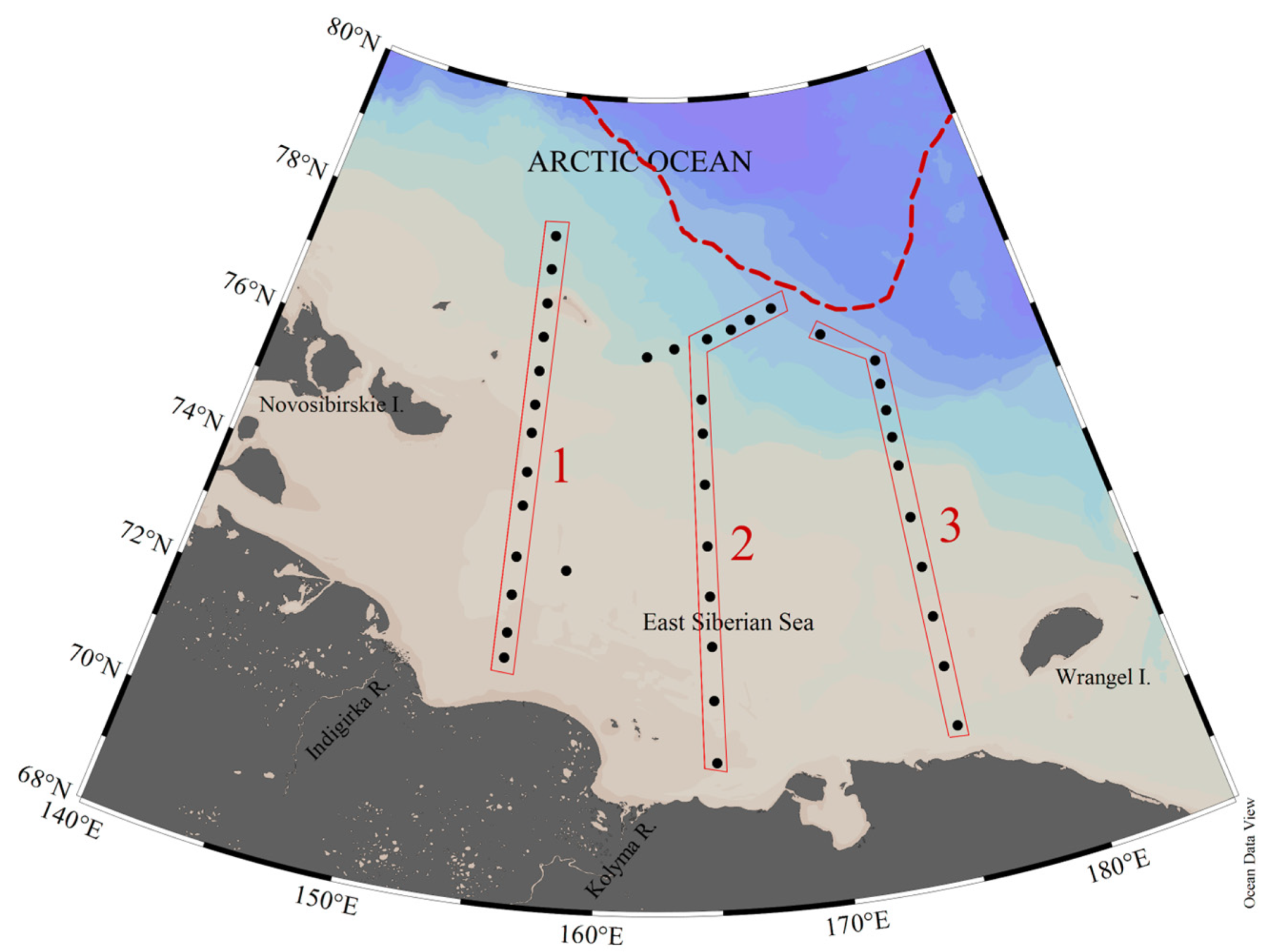
The ESS is the largest shelf sea in the Arctic Ocean [41], but it is the shallowest and has the smallest volume after the Chukchi Sea [42]. From a hydrographic point, the ESS is a transit area with seawater of Pacific origin entering from the east and water of Atlantic origin entering from the west [22]. The ESS is often divided in two regions: a western heterotrophic province, strongly influenced by the riverine runoff and products of the coastal ice complex erosion, and an eastern autotrophic province, influenced by the Pacific-origin inflow [18,27]. Recognizing the frontal zone around 165° E, we divided the study area into two regions: the western East Siberian Sea (W-ESS; from the New Siberian Islands to 165° E) and the eastern East Siberian Sea (E-ESS; from 165° E to the western shore of Wrangel Island).
Seawater samples were collected from the ESS continental shelf and slope from 25 September–4 October 2019 as part of the 90-day-long fourth stage of the TransArctic-2019 expedition onboard the RV “Professor Multanovsky” (Figure 1). The samples for chemical analysis were taken along the three inner shelf/coastal zone—slope transects (water depths ~15–310 m) at 39 stations in both provinces using a standard Rosette system equipped with the SBE911 + CTD (conductivity, temperature, depth) probe to record conductivity and temperature.
2.2. Methods of Measurements and Calculations
Water samples for total alkalinity (AT) were poisoned with a mercuric chloride solution at the time of sampling to halt biological activity [43] and were stored in the dark at room temperature until they were analyzed ashore. HgCl2-poisoned samples for AT were analyzed in the laboratory within 1 month using an indicator titration method in which 25 mL of seawater was titrated with 0.02 M HCl in an open cell according to [44,45]. Measurements of AT were performed at 20 °C with a precision of ~2 µmol kg−1 and the accuracy set by calibration against CRMs supplied by A. Dickson, Scripps Institution of Oceanography (USA). Batch no. 96 was used. pH was measured potentiometrically and reported on the total scale, having a precision of ±0.005 pH units [46]. At oceanographic stations, the partial pressure of CO2 (pCO2) and the aragonite saturation state (ΩAr) were calculated using the CO2SYS program [47] with equilibrium constants from [48] refit by [49].
Dissolved oxygen (O2) concentrations were obtained using a Winkler titration system, giving a precision ~1 μmol kg−1. These values were then converted to a percent saturation following [50]. Nutrients (dissolved nitrates, NO3−, silicates, Si, and phosphates, PO43−) were determined by traditional oceanographic techniques [51]. The samples were evaluated using a 6- to 8-point calibration curve at ~1% precision. Nutrient concentrations were used here as ancillary data to better estimate the derived parameters of the carbonate system (i.e., CO2 partial pressure [pCO2] and aragonite saturation state [ΩAr]) from directly measured parameters (i.e., pH and AT) as well as to clarify the carbonate system and water dynamics. A deficit in inorganic nitrogen relative to phosphate (N*, μmol kg−1) was calculated with equation proposed in [52] for water with a high ammonium concentration:
where ΣN (μmol l−1) is the total inorganic nitrogen concentration.
N* = (ΣN − 16 PO43− + 2.98) × 0.87,
The absorbance of CDOM was measured using a UNICO 2804 spectrophotometer with a 1 cm quartz cuvette over the spectral range from 200 to 600 nm at 1 nm intervals. Milli-Q (Millipore) water was used as the reference for all samples. Water samples underwent filtration through Whatman glass fiber filters (GF/F, nominal pore size 0.7 µm). The absorption coefficient (aλ, m−1) was calculated using equation aλ = 2.303 × Aλ/L, where Aλ is the optical density at wavelength λ, and L is the cuvette path length in meters. The absorption coefficients at 254 nm (a254) were chosen to quantify the concentrations of CDOM [53].
The equation published in [54] was used to calculate the CO2 flux (FCO2):
where K0 is the solubility of CO2 at the in situ temperature (mol m−3 atm−1), k is the gas transfer velocity (cm h−1), u is the daily average wind speed (m s−1), Sc is the Schmidt number for CO2 [54], and pCO2sw and pCO2air are the partial pressures of CO2 in equilibrium with surface water and in the above lying air, respectively. In situ monthly average pCO2air for September and October 2019 were taken from [55].
FCO2 = K0·k·(pCO2sw − pCO2air),
k = 0.251·u2 (660/Sc)0.5
The river water and sea ice meltwater contributions were quantified with a mass balance calculation, which was previously applied in the Arctic Ocean basins and shelf regions, using salinity and AT [33,56,57]. Assuming that the seawater sample is a mixture of Atlantic water (AW), sea ice meltwater (MW), and other fresh water (FW) that includes river runoff, precipitation, and fresh water carried by Pacific water, which has lower salinity than AW, the fractions of each end-member can be calculated using the following mass balance equations:
where S and AT are the observed salinity and total alkalinity of seawater, respectively, and f, S, and AT with subscripts are the fraction, salinity, and total alkalinity, respectively, of the three end-members of MW, FW, and AW. Each end-member value [57] is listed in Table 1.
fSW + fFW + fMW = 1,
SSW·fSW + SFW·fFW + SMW·fMW = S,
AT_SW·fSW + AT_FW·fFW + AT_MW·fMW = AT,
The normality of the data sets was tested using the Kolmogorov–Smirnov normality statistical test (K–S test). To measure the relationship between two variables, we used the Pearson’s correlation coefficient for normally distributed data.
Most of the plots and maps in this study were created with Ocean Data View software version 5.6.3 [58].
3. Results
3.1. Hydrometeorological Situation
3.1.1. Air Temperature
The mean near-surface air temperature (Tair) in winter 2019 in the marine Arctic was −20.5 °C [59]. The mean summer Tair (5.9 °C), was at the level of the highest Tair values (2012, 2016, and 2019). The annual average Tair in 2019 was −7.8 °C and ranked second in the series of so-called warm years after 2016 (−7.2 °C) (during the period of observation up to 2019).
3.1.2. Ice Cover
According to the National Snow and Ice Data Center (USA, NSIDC, https://nsidc.org/arcticseaicenews/ (accessed on 3 March 2023)), the Arctic sea ice extent in September 2019 was 3.1 million km2, which ranked third after the 2012 absolute minimum (2.4 million km2) and the 2007 minimum (2.8 million km2). The total anomaly of ice concentration relative to the average value in the observation period of 1981–2010 was negative; in September 2019 it was −1.6 mln km2, compared with −2.4 mln km2 in October of the same year. The position of the ice edge in the ESS in September 2019 is shown in Figure 1.
3.1.3. River Discharge
Along with the dynamics of ice area and thickness, the river runoff as one of the factors influencing the biogeochemical structure of the ESS waters is also subject to significant seasonal and interannual dynamics. The study was performed in late September–early October, when the riverine runoff that can influence the biogeochemical regime of the ESS waters (discharge of the Lena, Yana, Indigirka, and Kolyma rivers) was already significantly lower relative to the flood values (https://arcticgreatrivers.org/). The annual flow of the largest rivers (Lena and Kolyma) in 2019 (463 km3 and 89 km3) was also lower compared to the previous year (663 km3 and 140 km3) and compared to the long-term average for the 2000–2015 period (605 km3 and 94 km3 for the Lena and Kolyma rivers, respectively, [31]). For the Lena River, it comprised only 76% of the mean annual discharge and 70% of the discharge in the previous year; for the Kolyma River water, these values were 95% and 64%, respectively.
An increased share of winter runoff in the total river runoff became yet another interesting feature of these rivers’ hydrograph in 2019. Thus, for the Lena River, the mean annual contribution of winter runoff to the total volume was 8.5%, and in 2019, it was 14.3%, which was 126.9% of the 2000–2015 average. For the Kolyma River, these values were estimated at 6.6%, 8%, and 113%, respectively.
3.1.4. Sea Level Pressure
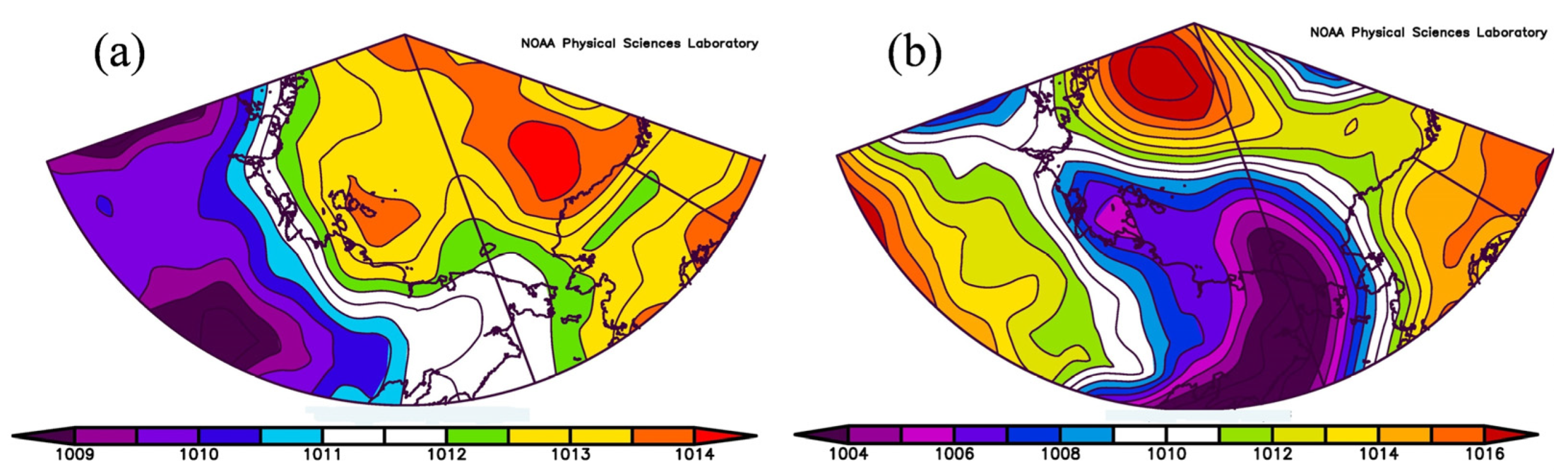
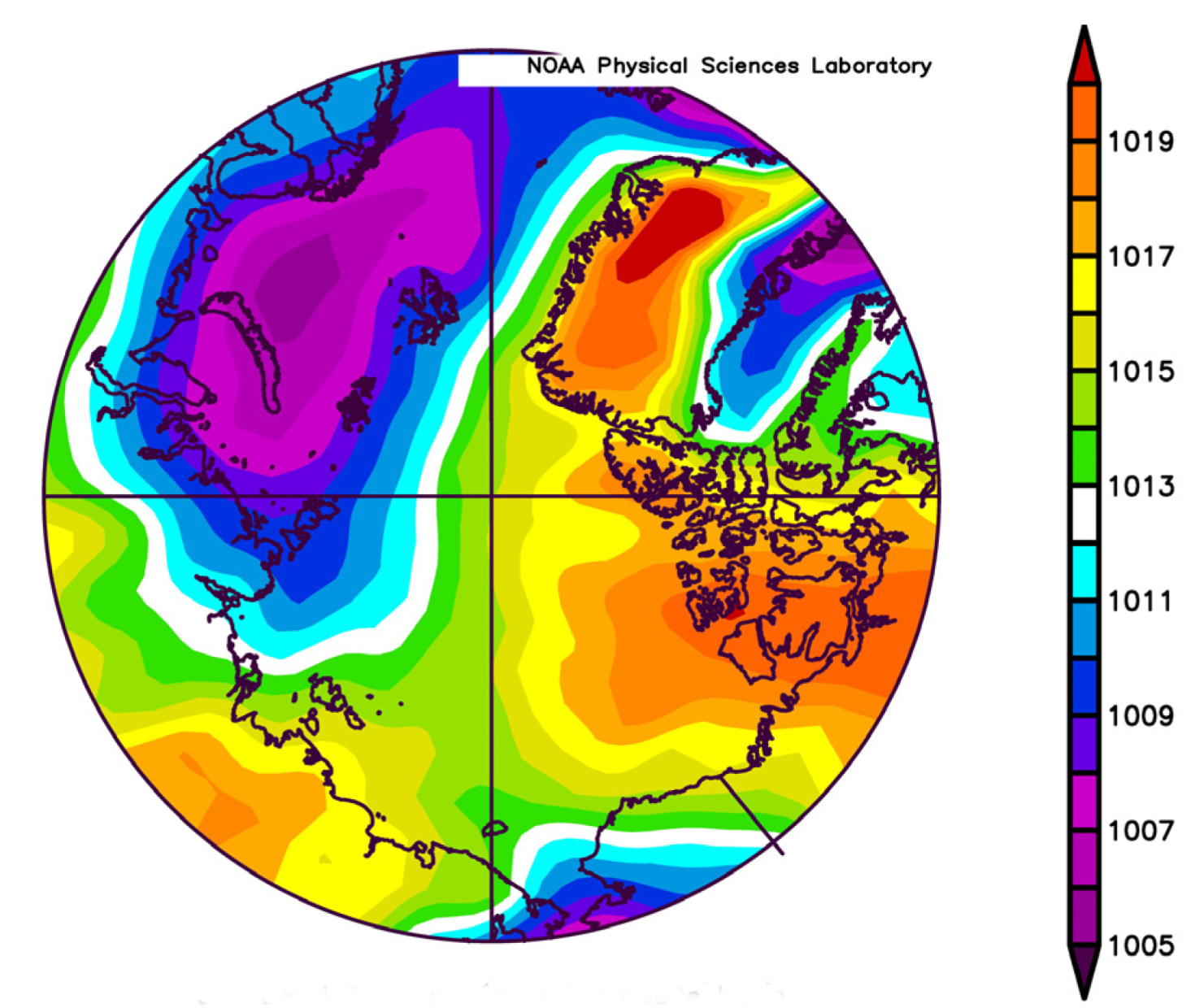
The analysis of the average surface pressure field (from National Centers for Environmental Prediction (NCEP) data, https://www.esrl.noaa.gov) for the warm season (the period of maximum river discharge) preceding the period of fieldwork revealed a weakly pronounced center of slightly elevated atmospheric pressure over the Novosibirsk Islands and the Beaufort Sea; in general, the atmospheric pressure field over the study area was low-gradient (Figure 2a) and to some extent contributed to the surface water transport in the W-ESS to the south and southwest and in the E-ESS to the west and northwest. During the study, a low sea level pressure dominated over the study area (Figure 2b), represented by a cyclone trough located over the continent. The westward and north-westward surface water transport dominated in the W-ESS while in the E-ESS, the westward and southwestward transport of surface waters prevailed; in the Chukchi Sea, it was westward and northwestward (https://www.esr.org/research/oscar/oscar-surface-currents/ (accessed on 16 May 2023)). At the same time, a cyclonic eddy existed over the outer shelf/slope in the E-ESS during the work.
The observed features of atmospheric circulation during the warm season contributed to the redistribution of surface waters freshened by the riverine runoff over the shelf in the western and northwestern directions, as well as to the transfer of Pacific-origin waters onto the ESS shelf and into the deep part of the sea.
3.2. Spatial Distribution of Studied Parameters
3.2.1. Lateral Distribution
The distribution of hydrological and carbonate parameters in the study area showed high spatial variability (Figure 3).
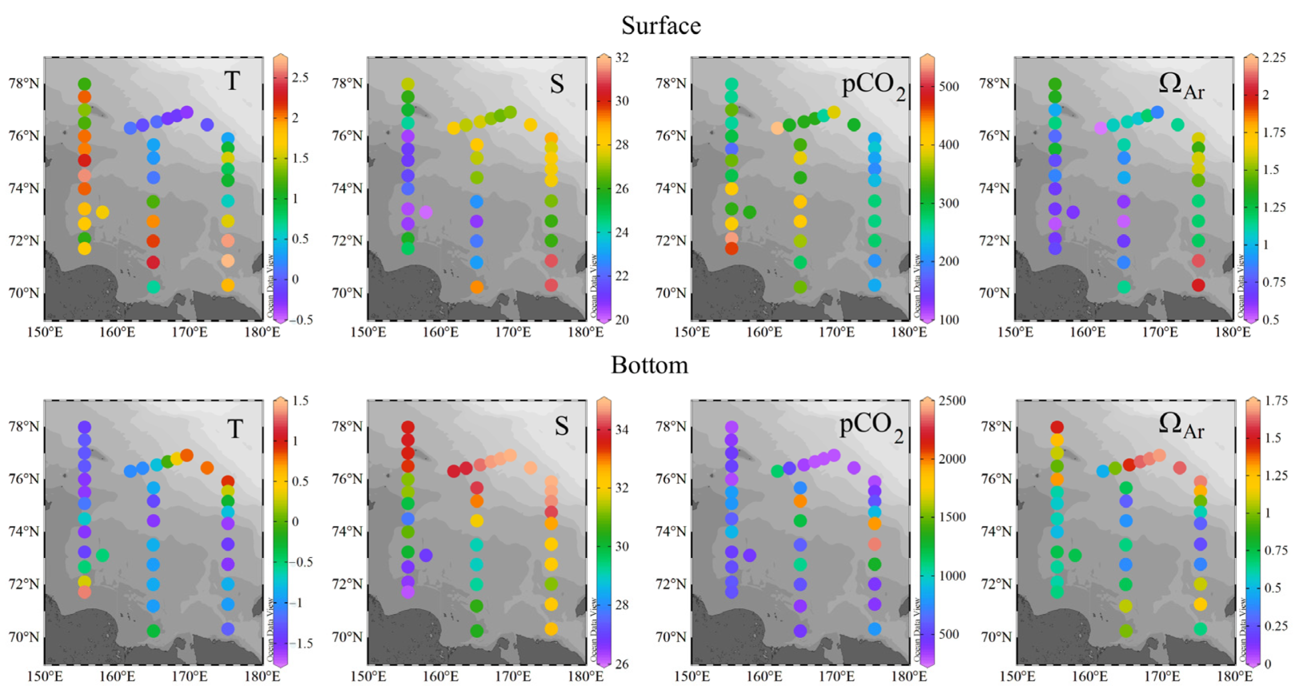
The surface water temperature expectedly decreased from south to north, reaching its minimum values near the ice edge (Figure 1 and Figure 3). The temperature fluctuations were opposite to the variability in salinity: the highest temperatures were observed in the zone of maximum freshening. In the bottom layer, both the temperature and salinity increased in the northeastern direction, reaching their maximum values in the zone of the greatest influence of transformed AW (Figure 3).
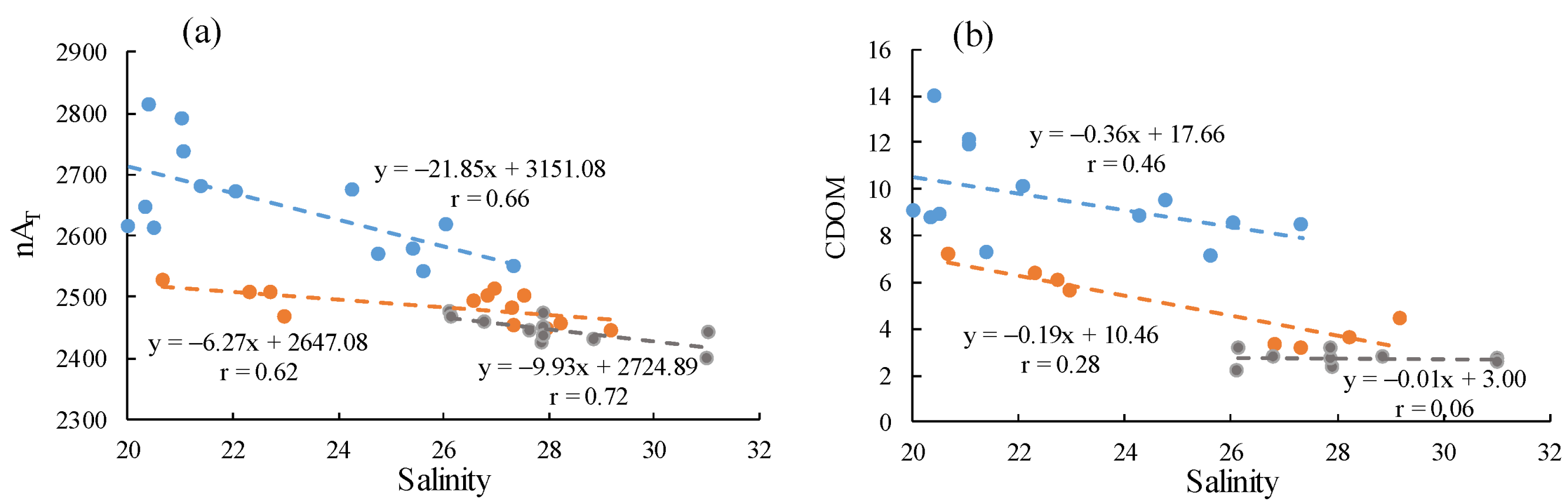
The waters freshened by the riverine runoff in the studied season had a limited distribution in the water area of the ESS as evidenced by the distribution of salinity and colored dissolved OM (CDOM) (Figure 3 and Figure 4) as well as normalized total alkalinity (nAT). Its mean values in the surface layer of the western, central, and eastern transects were 2651, 2484, and 2446 μmol kg−1, respectively. This is the typical response of the surface hydrography to atmospheric impacts when anticyclonic atmospheric processes prevail over the ESS during the warm season [20,25,27]. Another factor that determined the observed dispersion of river waters on the shelf was, as noted above, the reduced riverine runoff. In the surface layer of the W-ESS, the calculated content of river waters reached 33%; in the east and northeast of the sea, it dropped below 10%.
Thus, the greatest contribution of river waters was observed in the surface layer of the western transect (Figure 3 and Figure 4); the contribution was twice that of sea ice melt waters. In addition, we can differentiate the contribution of the Lena and Kolyma waters on the graph of the dependence of nAT and CDOM on salinity in the western transect: the former are characterized by higher values of nAT and CDOM [25,60]. It has weakened the relationship between these parameters and surface salinity in the western transect (Figure 4). Further to the east, the influence of the riverine runoff weakened. In the eastern transect, the upper layer freshening was significantly associated with sea ice melt water (Figure 3 and Figure 4). This was confirmed by the predominant character of atmospheric circulation and the direction of surface currents (https://www.esr.org/research/oscar/oscar-surface-currents/ (accessed on 16 May 2023)), as well as the estimated fractions of river and sea ice melt waters.
In the surface layer of the ESS, the ΩAr values varied from 0.50 to 2.08, and pCO2—from 203 to 534 μatm. The minimum values of pCO2 and maximum values of ΩAr were observed in the E-ESS, where the influence of highly productive Pacific waters was significant. The highest oxygen saturation (up to 99% in the surface layer and up to 118% in the subsurface) was also observed here. Maximum surface pCO2 values and the minimum ΩAr values were found in the W-ESS, the zone of intense terrestrial water dispersion that influences coastal ice complex erosional products.
A major part of the entire bottom layer waters was calcium carbonate corrosive: the ΩAr values were significantly below 1, which is the equilibrium value below which the dissolution of aragonite occurs. The exception was the bottom waters of the outer shelf in the northwest and the continental slope in the northeast of the sea, where the ΩAr values reached 1.68 (Figure 3). Extremely low values (ΩAr = 0.22) were observed in the bottom layer of the eastern province; these values were accompanied by the maximum values of pCO2 (2400 μatm).
3.2.2. CO2 Fluxes in the Ocean–Atmosphere System
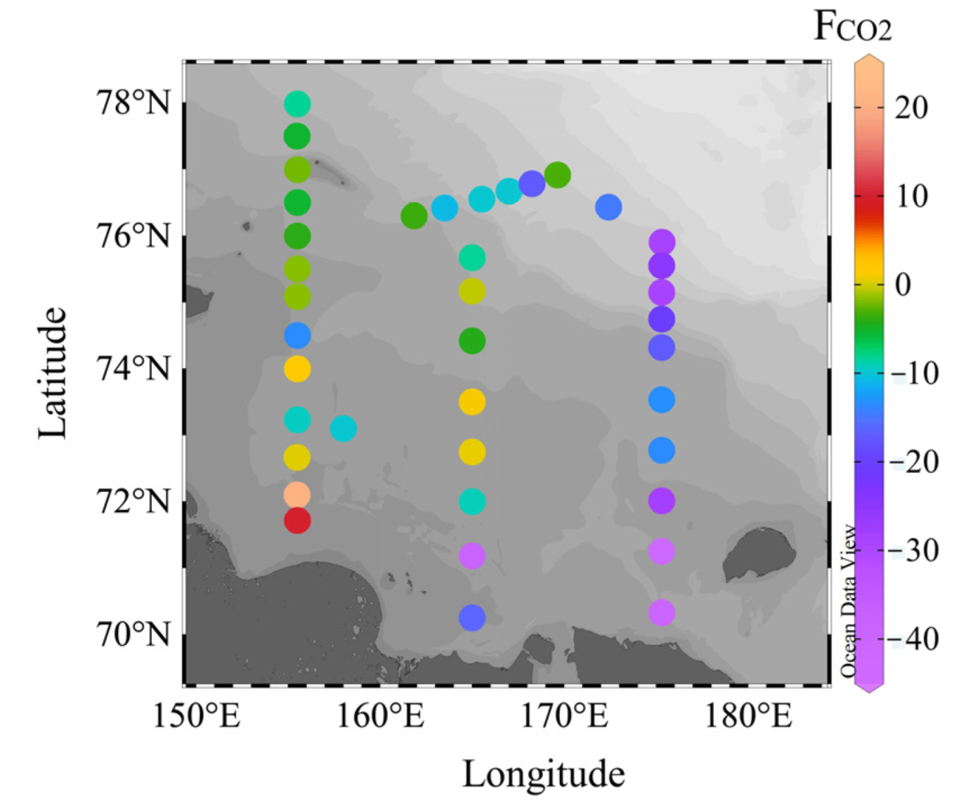
The estimated values of the air–sea CO2 fluxes showed that, in general, in the late autumn season the ESS was a sink for atmospheric CO2 (Figure 5), and the CO2 flux into the seawater averaged for the entire study area was 11.2 mmol m−2 day−1. The most intense CO2 uptake occurred in the eastern autotrophic part of the sea (Figure 5, Table 2) with a maximum rate of 43.8 mmol m−2 day−1. The CO2 flux was directed into the atmosphere only in the restricted coastal zone of the W-ESS, which was most influenced by river runoff and the products of coastal erosion (Figure 5); the maximum CO2 outgassing rate here reached 20.5 mmol m−2 day−1.
3.2.3. Vertical Structure of the Water Column
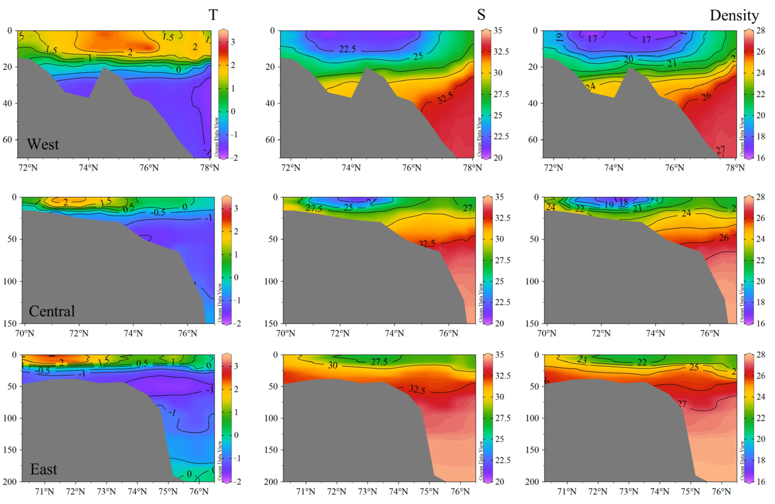
The vertical distribution of the studied parameters in the three meridional transects differed significantly and had distinctive features in each of them (Figure 6 and Figure 7). The entire ESS was vertically stratified, though less pronounced in the east due to the diminishing influence of the riverine runoff.
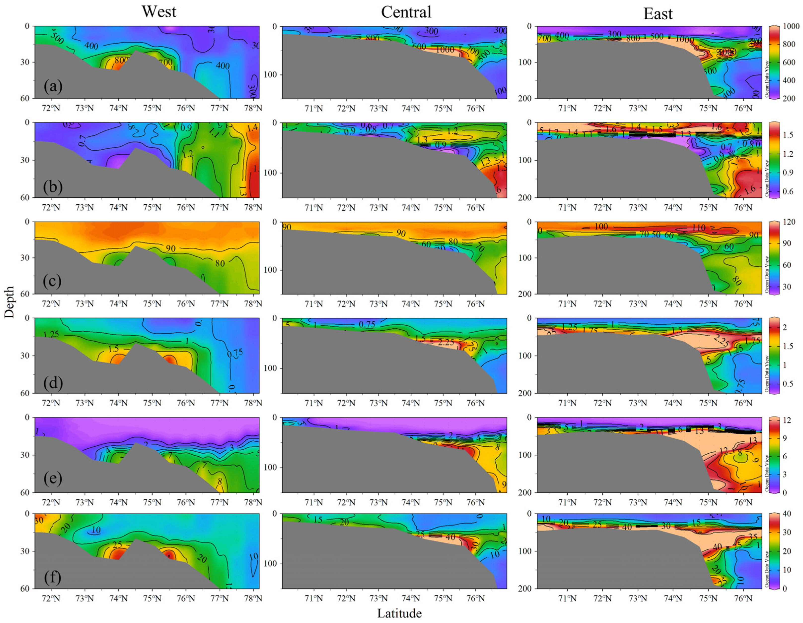
The waters of the western transect (transect 1) had strong stratification and the sharpest pycnocline separating the upper mixed layer from the lower horizons (Figure 6). The strong stratification restricted the vertical replenishment of surface nutrients (Figure 7). No trend was revealed in the distribution of surface temperature along the transect, and salinity only slightly increased to the north. The surface layer was the most freshened compared to the other two transects. The maximum temperature of the western transect measured in the subsurface at a depth of 10 m was 3.12 °C (Figure 6). Surface waters were depleted of nutrients, except for silicates; the oxygen saturation level did not reach equilibrium values (Figure 7). The maximum values of the latter were 101%, observed at a depth of 15 m, and the minimum (61%) was found in the bottom layer. The entire water column of the inner shelf and part of the middle shelf (up to the depth of 40 m) were calcium carbonate corrosive with the minimum ΩAr value of 0.51 observed in the bottom layer. The maximum oversaturation of waters with CO2 was found in the south of the transect (534 μatm) while to the north, pCO2 values went down to 266 μatm. The average AT value in the water column was 1944.6 ± 235.6 μmol kg−1, pH—8.00 ± 0.12 pH units, pCO2—396 ± 134 μatm, ΩAr—0.96 ± 0.30.
Transect 2, made in the central part of the sea, showed the continuing trend of decreasing surface water temperature from south to north, with slight fluctuations associated with the presence of the freshwater lens in the southern/central part of the transect. Minimum salinity was observed in the freshwater lens (Figure 6), and some decrease was observed in the north near the ice edge. The concentrations of nutrients (NO3− and PO43−) in the surface layer were low; the exception was the shallow coastal station (Figure 7). As in transect 1, the water column of the inner shelf and almost the entire middle shelf was calcium carbonate corrosive. The values of pCO2 in the surface layer, except for a few points in the south of transect, were close to or below the equilibrium values, reaching a value of 264 μatm in the north. The average AT value in the water column was 2078.4 ± 195.4 μmol kg−1, pH 8.01 ± 0.15 pH units, pCO2 421 ± 238 μatm, and ΩAr 1.09 ± 0.33.
An intermediate layer of corrosive waters appeared on the outer shelf at depths of 40–70 m, and further observations at all northern stations of the transect indicated a characteristic feature of the distribution of the studied characteristics in the central transect (Figure 7). It had low ΩAr values, not exceeding 0.75 even at the northern stations, high values of pCO2, significant oxygen undersaturation, and elevated concentrations of nutrients. The temperature in the layer of these waters was below zero (below −1.14 °C), and the salinity varied in the 32–33.5‰ range.
In the eastern transect 3, the waters were also stratified; however, the vertical gradients of hydrological characteristics were much smaller compared to the western and central transects (Figure 6). Surface temperature, like salinity, tended to decrease from south to north. The latter was significantly higher compared to the western transects. Surface waters were oversaturated in calcium carbonate, especially in the southern part of the transect, and undersaturated in CO2: pCO2 dropped to 202 μatm. The average AT value in the water column was 2144.3 ± 142.6 μmol kg−1, pH 8.05 ± 0.22 pH units, pCO2 435 ± 366 μatm, and ΩAr 1.29 ± 0.45.
The vertical hydrochemical structure had several outstanding features. The first was the occurrence of oxygen-oversaturated (up to 119%) waters with sub-zero temperature (down to −1.4 °C), salinity 31.0–31.9‰, pCO2 values of 183 μatm, and ΩAr 2.09 at depths of 20–30 m. The second was the layer of intermediate corrosive waters at depths of 40–70 m with low temperatures (from −1.7 to −1.2 °C), salinity of about 32.2–33.5‰, a low oxygen content, and high concentrations of nutrients that were more clearly traced (Figure 7). In the deep part of the transect, the N/P ratio increased with increasing salinity, approaching the Redfield ratio in the zone of maximum influence of the AW.
4. Discussion
4.1. Spatial Dynamics of Carbonate Parameters on the Shelf
In the late autumn season, most of the surface waters of the ESS were undersaturated with CO2 relative to the atmosphere and served as a sink for atmospheric CO2. At the same time, the waters of the eastern autotrophic part of the sea, as in the summer–autumn season [22,23,25], showed significantly lower pCO2 values—the average pCO2 value in the surface layer of the western transect was 1.5 times higher compared to the eastern one. Oversaturation relative to the atmospheric CO2 level was observed only in the surface waters of the shallow southwestern part of the W-EES. This spatial distribution was caused by a few factors. Firstly, the total river runoff in the ESS was significantly lower than the long-term annual average volume; moreover, the work was carried out during a seasonal decrease in riverine discharge. Secondly, the prevailing atmospheric circulation in the warm season did not contribute to the intensive spreading of river water over the sea area or to the transfer of these waters and the products of erosion of the coastal ice complex eastward. A cyclone was located directly over the southeastern part of the sea (Figure 2), determining the inflow of waters from the Chukchi Sea mainly north of Wrangel Island to the ESS. Thirdly, the autumn cooling of waters had already started (Figure 6), reducing the values of the surface water’s pCO2. It should be noted that autumn cooling and water convection were limited to the uppermost horizons. Thus, the cooling of waters decreased the pCO2 of surface waters, decreased fluxes to the atmosphere in the coastal W-ESS, and increased fluxes to the seawater in the E-ESS. Moreover, in the E-ESS, subsurface layers with even lower pCO2 (and high oxygen saturation) that formed because of photosynthesis processes were involved in the exchange processes because of the beginning of autumn mixing. At this time there was no CO2 inflow from deep layers enriched with inorganic carbon to the surface layers. Thus, we observed a seasonal phenomenon: the initial stage of autumn convection in the productive eastern part of the sea caused an additional biological decrease in surface pCO2. Note that the entire water column at the shallow stations near Wrangel Island was well aerated and undersaturated by CO2. The intensification of photosynthesis processes here could most probably be attributed to the upward inflow of nutrients into the photosynthesis zone because of the cyclonic movement of waters coming from the Chukchi Sea and the high transparency of the water column.
Despite the sharpest pycnocline in the W-ESS (Figure 6), which hindered exchange processes, the maximum values of pCO2 (up to 2400 μatm) accompanied by extremely low oxygen saturation (~20%) and maximum silicate concentrations (up to 84 μmol L−1) were found in the bottom layer of the eastern province, greatly influenced by the waters of Pacific origin (Figure 3 and Figure 7). Intense photosynthetic processes in the E-ESS [22,25] were a permanent source of labile autochthonous OM to the underlying water column and bottom sediments. Fresh OM derived from marine plankton has prevailed in the E-ESS sediments and in the particulate organic carbon pool [38]. Therefore, the contribution of terrestrial organic carbon to particulate organic carbon reached 99% in the W-ESS, but accounts for as low as 1% in the E-ESS [38]. The waters of Pacific origin that also carried a labile OM fraction [38] were additionally modified on the ESS shelf owing to the interaction with the bottom sediments containing fresh autochthonous OM as well as relatively labile (compared to the western province) allochthonous OM [61]. Matsubara et al. [61] showed that river-transported terrestrial OM from surface soils, which is less resistant to degradation compared to the erosion-derived terrestrial OM from ice complex deposits of the seashore and riverbank [29,30,62], prevails in the terrigenous component of the E-ESS bottom sediments. For example, the degradation rate in the bottom sediments of lignin phenols coming to the shelf, mainly from seasonally melted soils, is three times as high as the degradation rate of the total sedimentary terrigenous OM pool [61].
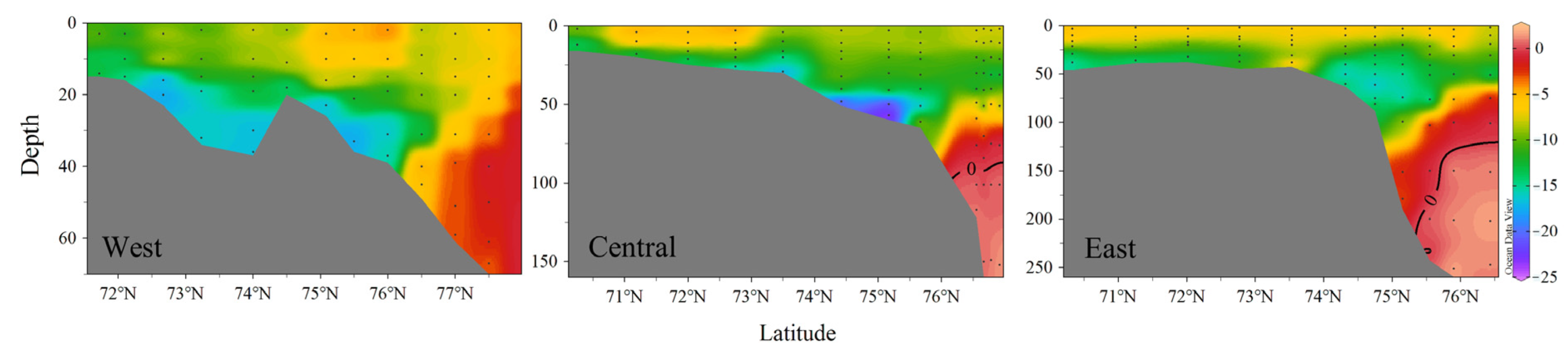
The interaction of waters with bottom sediments of the ESS shelf was evidenced by low N* values [52]. Both OM decomposition and denitrification occur within the shelf sediments, and the diffusion of pore water from the sediments reduces oxygen concentrations and N* values in the bottom waters [57]. The observed low N* values (down to −26 μmol L−1) were indicative of processes of OM decay under the low oxygen conditions of the bottom layer of shelf waters (Figure 8).
As noted above, in late autumn, a significant part of the ESS shelf waters was calcium carbonate corrosive, and the area of these waters was not limited to the surface or near-bottom layer. In the W-ESS, inner and middle shelf waters were undersaturated with aragonite throughout the entire water column (Figure 7) owing to the strong influence of the terrigenous runoff through the riverine inflow and coastal erosional OM. In the E-ESS, bottom waters up to the shelf break were characterized by low (below 1) ΩAr values, determined by the fresh (mainly marine) OM decay, and the depth of the isoline ΩAr = 1 here was about 35–40 m. Only three zones were an exception for near-bottom waters. Firstly, at the shelf stations near Wrangel Island, where the production processes in the incoming waters of Pacific origin decreased the CO2 content in the entire water column and, consequently, the level of corrosivity (ΩAr increased to 1.17 in the bottom layer). Secondly, the influence of AW of the boundary current flowing along the Siberian continental slope (with S~34.7–34.8‰ and T~0–1 °C) determined the oversaturation of bottom waters with aragonite at the northern stations of the central (2) and eastern (3) transects. It is important that we also found cold (with temperature below zero) highly saline waters with a slight signature of contact with bottom sediments (S~34.5–34.6‰, T from −0.68 to −0.26 °C, O2~58–74%, N* from −2.7 to −0.5 μmol L−1, Si~15–23 μmol L−1, NO3−~10.2–12.9 μmol L−1), and those without it (S~34.3–34.7‰, T from −1.26 to −0.03 °C, O2~83–86%, N*~0.2–1.7 μmol l−1, Si~4.5–11.4 μmol l−1 and NO3−~7.2–9.7 μmol L−1), characterized by ΩAr values higher than 1 (1.14–1.69). The latter waters without a signature of any nutrient maximum have historically been named lower halocline water, LHW [40,63], and the basin waters in the Chukchi Abyssal Plain most likely were the source of the former waters [40]. Thirdly, incoming waters from the outer shelf of the Laptev Sea (with salinity ~33.6‰ and T from −1.4 to −1.26 °C, [64]) increased the ΩAr values in the entire water column, including the bottom layer, in the north of the western transect (1) (Figure 7).
The processes of photosynthesis at depths of ~20–30 m in the middle and outer shelf and on-slope waters were a significant factor determining the formation of increased ΩAr values in the surface/subsurface layer in the E-ESS. These waters were enriched by nutrients because of the interaction with shelf bottom sediments, as evidenced by negative N* values (from −14.3 to −7.9 μmol L−1). Under conditions of sufficient solar radiation owing to the prolonged onset of freeze-up, intensive processes of primary production have developed here. The waters of this layer in the outer shelf and on-slope waters had 31–31.9‰ salinity, below-zero temperatures, high oxygen saturation (up to 118%), and ΩAr values up to 2.09 and occupied the uppermost part of the cold halocline that was identified in the deep part of the sea as upper halocline water (UHW). It was shown that UHW mainly resulted from advected fresh East Siberian cold shelf water or fresh Pacific winter waters [40,57,65]. Thus, the UHW in 2019 could have been formed by the modification of the Pacific-origin summer shelf waters through winter cooling and convection in the shelf areas, where the winter freeze-up has been significantly delayed recently. In October 2018, an extensive area of the open water occurred in the E-ESS and in the western Chukchi Sea, allowing for heat loss from the water to the atmosphere and resulting in the formation of cold water by cooling and convection [40,57,66].
It is likely that one of the additional factors that cause intensive photosynthetic processes in the oligotrophic on-slope waters of the northern part of the ESS was the influx into this area of highly saline waters of LHW [66]. LHW lifted Pacific-origin waters enriched with nutrients up to the zone of light intensity suitable for photosynthesis, leading to anomalously high phytoplankton blooms in typically oligotrophic waters. The predominant atmospheric circulation in the preceding winter and spring seasons (November 2018–May 2019)—a deep cyclone over the Barents and Kara seas and a weak anticyclone over the Beaufort Sea (Figure 9)—could determine the spread of LHW far to the east. The position of the boundary between positive and negative N* values confirmed this assumption (Figure 8): the N* profiles clearly showed the substantial shoaling of the Atlantic-origin water upper boundary (positive N* values [52]) to depths of at least 130–150 m (the sampling discreteness does not allow a more precise estimate) with its typical position at ~300–320 m [66]. A similar location of the upper boundary (~140 m), determined by the circulation pattern (the cyclonic atmospheric circulation was considerably strengthened during the winter/spring season) was observed in 2017 in the on-slope waters of the northwestern Chukchi Sea [66]. Note that the gradual shoaling of the AW was shown in the Eurasian Basin (a process called “Atlantification”) [67], and a similar process is now impacting the western Amerasian Basin, reaching the Chukchi Borderland [65].
In addition to the shoaling of the corrosion layer caused by LHW intrusion, ice retreat beyond the shelf break also provided favorable conditions for upwelling along the shelf break [68]. As a result, nutrient-rich deep waters could also enter the surface layers of the northeast ESS [66,69]. It can be assumed that upwelling probably occurred during the fieldwork, supplying additional nutrients to the photic layer and contributing to the intensification of phytoplankton blooms.
At the northernmost station near the ice edge, the maximum oxygen oversaturation (104%) was shoaled and observed at the 10 m horizon. Enhanced phytoplankton production, indicated by oxygen saturation maxima and nitrate minima, “was found associated with and primarily controlled by (in the presence of light and nutrients) enhanced density stratification and frontal structure in the marginal ice edge zones due to ice melt” [70]. Wind-driven ice edge upwelling may also have supplied nutrients for phytoplankton production [70].
In the surface layer, the correlations of ΩAr values with pCO2 and salinity were equally strong: in the first case, the correlation coefficient was −0.81, and in the second, 0.81, which indicated a similar level of influence of hydrological (salinity) and biochemical (pCO2) factors on ΩAr distribution. This also showed that the physical movement of water and the production/degradation of OM were the dominant drivers of the ΩAr variability in the surface layer. In the bottom layer, the relationship between ΩAr and salinity weakened (r = 0.52) while remaining consistently strong (r = −0.75) with pCO2, indicating the dominant influence of biochemical processes on the ΩAr dynamics. Here, the main driver of ΩAr variability was OM degradation: low values of ΩAr were associated with high values of pCO2 (and low pH), high concentrations of nutrients, and low level of oxygen saturation, indicating the importance of OM degradation in controlling the chemical composition of shelf bottom waters.
Thus, the general main factors that contributed to the observed variability in the carbonate system parameters and aragonite saturation state of ESS waters included the influence of waters of different salinity and OM decay. In the western heterotrophic province, the predominant freshening of the surface layer was determined by the terrestrial runoff, and the OM was, to a large extent, of terrigenous origin. In the eastern autotrophic province, the significant contribution to surface layer desalinization was made by sea ice melt water while the degrading OM was predominantly autochthonous, and primary production processes additionally influenced the level of water corrosivity with respect to calcium carbonate.
The existence of an intermediate layer of waters undersaturated with respect to calcium carbonate at depths greater than 40 m was a characteristic feature of the E-ESS waters in late September to October 2019. Their brightest signal was detected along the easternmost transect; it was less pronounced in the central transect, and we did not find similar extremes in the intermediate waters in the W-ESS during our work (Figure 7). We observed extreme values of the studied parameters (the lowest values of pH, ΩAr, and oxygen saturation and the highest values of pCO2 and dissolved silicates) in the bottom layer of the E-ESS shelf. These waters spread over the outer shelf and slope of transects 2 and 3 with gradual weakening of the corrosive water’s signature in the deep sea. The data obtained allowed us to conclude that the E-ESS can be considered a source of the oxygen-depleted and nutrient-enriched corrosive waters for the deep part of the sea and the Arctic Ocean in general.
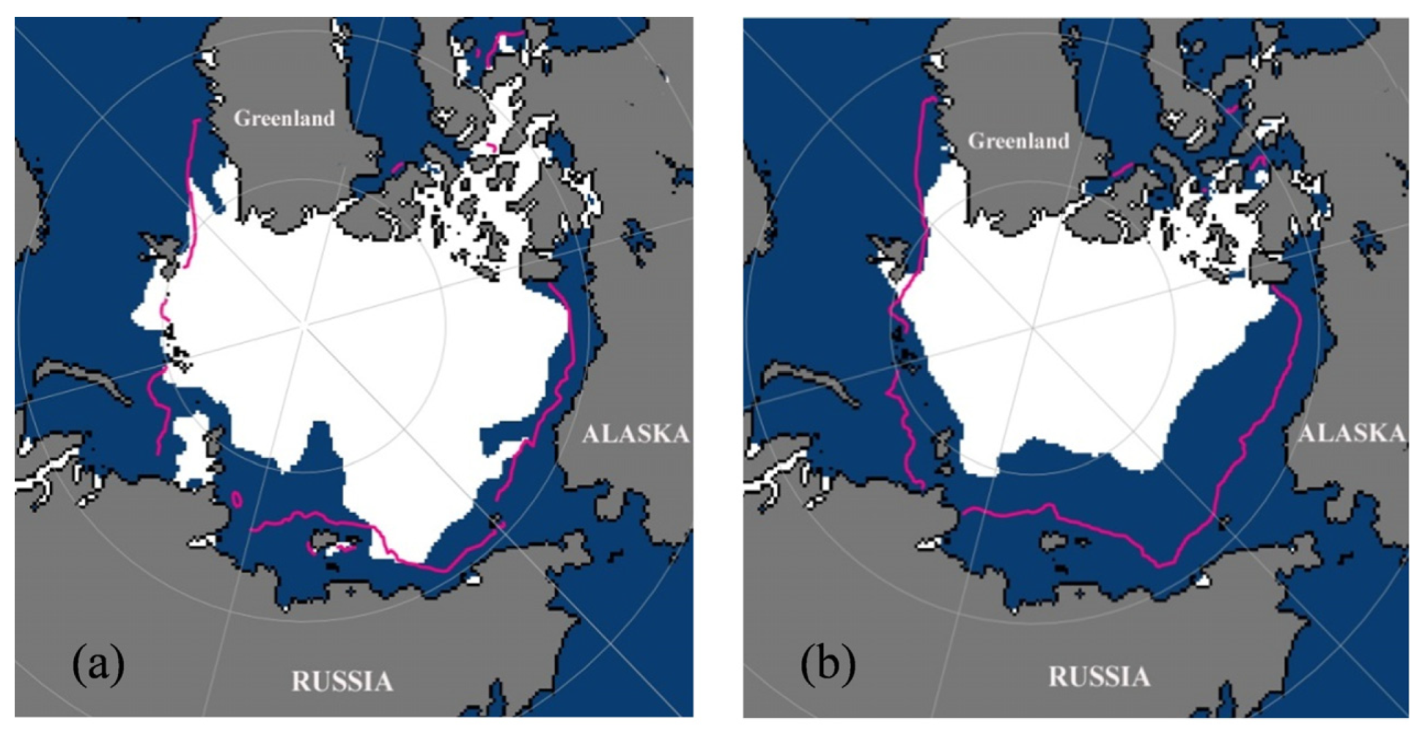
Previously, Anderson et al. [34,40] showed that calcium carbonate corrosive and high-nutrient water with salinity centered at 33‰ exited the ESS from its western end and contributed to the cold halocline of the central Arctic Ocean. Compared to historic data, the high-nutrient water was found outside the shelf break further to the west in 2014, which was associated with a lower degree of ice cover during the summer north of the New Siberian Islands [40]. In the autumn of 2019, sea ice cover had significantly less extent over the ESS compared to 2014 (Figure 10). The most significant reduction of the sea ice area occurred in the central and eastern parts of the sea. Thus, during our work in 2019, cold corrosive waters entered the deep part of the sea and further into the Arctic Ocean from the eastern, less ice-covered part of the sea (Figure 10).
A significantly smaller ice cover area in 2019 compared to 2014 in the E-ESS (Figure 10) was the important factor, which allowed the wind to drive the ocean circulation more effectively. An intensification of photosynthesis processes in the 20–30 m layer in the eastern deep part of the E-ESS could additionally contribute to the corrosivity of the upper Pacific-origin halocline waters because of synthesis and the subsequent degradation of freshly formed OM.
Thus, owing to the dynamics of currents caused by the predominant atmospheric circulation and a large area of open water, as well as the presence of more labile OM in the bottom sediments and water column in the E-ESS, this area was a source of corrosive water to the deep ocean in late autumn 2019.
4.2. CO2 Fluxes between the Seawater and the Atmosphere
A comparison of the estimated values of CO2 fluxes between the water and the atmosphere showed that in the eastern autotrophic province, the average and absolute fluxes of CO2 into the seawater were significantly higher than the values calculated for the western heterotrophic part of the sea (Table 2). Given that the difference in pCO2 values between surface water and air is the parameter determining the flux direction in the ocean–atmosphere system and the distribution of pCO2 values in the atmosphere is quasi-stable relative to the dynamics of seawater pCO2, the evasion and invasion zones were regulated by the same factors that determined the pCO2 dynamics of surface water. For the W-ESS, these factors included the influence of CO2-enriched riverine waters and the decomposition of terrigenous OM delivered with continental waters and contributed by the erosion of the coastal ice complex, as well as synthesized in situ. For the E-ESS, it was the CO2-depleted sea ice melt waters, highly productive waters of Pacific origin, the intensive processes of photosynthesis in the subsurface layer (and in the surface one for the station near the ice edge), and the destruction of OM mainly of autochthonous genesis. As a result, the absolute value of ΔpCO2 was more than three times as high in the east of the study area (Table 2). The difference in water temperature at transects could have played a certain role, but it was extremely small (average surface water temperature was 1.77, 0.60, and 1.27 °C along transects 1–3, respectively). Therefore, the contribution of temperature variability between transects was insignificant both in the spatial dynamics of ΔpCO2 and Sc, a parameter that influences the gas transfer velocity. The intensity of the CO2 flux also depends on the atmospheric circulation-related wind speed, which was significantly higher in the E-ESS (Table 2). A cyclone over the southeast ESS and an anticyclone over the northeast determined a high-gradient field of atmospheric pressure (Figure 2) and, consequently, higher wind speeds along transects 2 and 3 compared to transect 1. The resulting average flux of CO2 from the atmosphere to the seawater along the eastern transect was three times as high as that along the central transect and an order of magnitude larger than that along the western transect.
As a result of the current hydrometeorological situation, the area of the CO2 uptake in the ESS was significantly increased compared to that observed earlier in the late summer season [22,23,25,32,36,37]. We compared the values of air–sea CO2 fluxes calculated in 2019 with the values calculated in September 2008 [25]; in both cases, the fluxes were assessed using the parameterization of Wanninkhov et al. [54] and daily averaged wind speed. September 2008 was chosen for comparison, since in 2008, the biggest area of the atmospheric CO2 uptake for the summer season was identified in the ESS shelf waters during our field work, and the study area covered both biogeochemical provinces of the ESS [25]. In the summer of 2008, an atmospheric anticyclone prevailed over the Chukchi and Beaufort seas, and the cyclonic circulation was not developed over the ESS. Predominant atmospheric circulation led to the westward dispersion of the Pacific-origin waters. This significantly increased the area of the autotrophic province in the ESS. At similar values of ΔpCO2, the rates of CO2 uptake before the onset of freeze-up in 2019 were higher compared to those in the late summer of 2008 (Table 3). The main reason for the higher CO2 fluxes was the dynamic factor—the daily averaged wind speed in autumn 2019 reached 7.25 m s−1 with a maximum daily value of 11.9 m s−1, which was almost double the values measured in 2008 (Table 3).
It is important that in the late autumn season, a significant undersaturation of surface water with CO2 relative to the atmosphere observed earlier in different parts of the Arctic continental slope [33,34,35,71,72,73] also persisted. This allowed us to identify this area as a permanent sink for atmospheric CO2 during the warm season.
Thus, shortly before ice formation (freeze-up processes started less than one week after our work in the ESS, https://nsidc.org/arcticseaicenews/ (accessed on 3 March 2023)), the ESS as a whole was a strong sink for atmospheric CO2.
5. Conclusions
Data obtained during a late autumn cruise allowed us to conclude that under the conditions of the limited dispersion of riverine water caused by its reduced discharge (reduction of both mean annual and seasonal discharge) and by prevailing cyclonic atmospheric circulation over the easternmost part of the sea, the ESS was predominantly a strong sink for atmospheric CO2. The beginning of the autumn cooling of water and phytoplankton blooms in the E-ESS were additional drivers of the increased seawater CO2 uptake. The development of photosynthesis processes was found even in the oligotrophic waters northeast of the sea. Phytoplankton blooms in the absence of intensive autumn convection were caused by the specific dynamics of waters of different genesis determined by atmospheric circulation both in the preceding seasons and directly during the field research.
In the late autumn season, a significant part of the ESS surface waters (predominantly in the heterotrophic western province) was calcium carbonate corrosive. The waters of the bottom layer turned out to be most corrosive to calcifying biota. These waters had a low saturation state with respect to calcium carbonate down to 0.22 for aragonite, and the area of corrosive waters covered almost the entire shallow shelf. Extremely low ΩAr values were found in the bottom layer of the E-ESS, and the E-ESS was the main source of corrosive waters to the deep ocean during the late autumn season in 2019. This was determined by a high content of fresher and more labile OM in the water column due to the waters of the Chukchi Sea and in situ synthesis, the prevalence of marine OM in sediments, the features of the sea ice extent, and the atmospheric/seawater circulation. The observed transport of corrosive shelf waters in the subsurface layer to the deep part of the ocean can have a potential impact on the ecosystem of oceanic waters in the case of mixing with the layers inhabited by calcifying organisms.
The datasets of the study presented here are small to fully explore the modulating effects of different processes on the carbonate chemistry variability throughout the entire late autumn season. However, these are the first data characterizing the state and driving forces of the dynamics of the seawater carbonate system and waters corrosive to calcifying biota from the shallow inner shelf to the continental slope of two contrasting biogeochemical provinces of the ESS, obtained shortly before autumn ice formation.
Author Contributions
Conceptualization, I.P. and S.P.; methodology, I.P. and I.S.; formal analysis, S.P. and O.K.; investigation, S.P., O.K. and I.P.; writing—original draft preparation, I.P., S.P., I.S. and O.K.; writing—review and editing, I.P. and S.P.; visualization, S.P.; funding acquisition, I.P. All authors have read and agreed to the published version of the manuscript.
Funding
This research was funded by the Russian Science Foundation (RSF, project No. 21-17-00027).
Data Availability Statement
All data are presented in the article in tables and graphics.
Acknowledgments
The authors are grateful to the Administration of the Far Eastern Regional Hydrometeorological Research Institute for the materials provided.
Conflicts of Interest
The authors declare no conflict of interest.
References
- Jorgenson, M.T.; Brown, J. Classification of the Alaskan Beaufort Sea Coast and estimation of sediment and carbon inputs from coastal erosion. Geo Mar. Lett. 2005, 482, 32–45. [Google Scholar] [CrossRef] [Green Version]
- Manson, G.K.; Solomon, S.M. Past and future forcing of Beaufort Sea coastal change. Atmos. Ocean 2007, 45, 107–122. [Google Scholar] [CrossRef]
- Stroeve, J.; Notz, D. Changing state of Arctic sea ice across all seasons. Environ. Res. Lett. 2018, 13, 103001. [Google Scholar] [CrossRef]
- Timmermans, M.-L.; Labe, Z. Sea Surface Temperature. In Arctic Report Card; Update to 2020; National Oceanic and Atmospheric Administration (NOAA): Washington, DC, USA, 2020. [Google Scholar] [CrossRef]
- AMAP Assessment 2013: Arctic Ocean Acidification; Arctic Monitoring and Assessment Programme (AMAP): Oslo, Norway, 2013; Available online: https://www.amap.no/documents/doc/amap-assessment-2013-arctic-ocean-acidification/881 (accessed on 1 December 2013).
- AMAP Assessment 2018: Arctic Ocean Acidification; Arctic Monitoring and Assessment Programme (AMAP): Tromsø, Norway, 2019; Available online: https://www.amap.no/documents/doc/amap-assessment-2018-arctic-ocean-acidification/1659 (accessed on 10 October 2018).
- Steiner, N.S.; Bowman, J.; Campbell, K.; Chierici, M.; Eronen-Rasimus, E.; Falardeau, M.; Flores, H.; Fransson, A.; Herr, H.; Insley, S.J.; et al. Climate change impacts on sea-ice ecosystems and associated ecosystem services. Elem. Sci. Anth. 2021, 9, 00007. [Google Scholar] [CrossRef]
- Aagaard, K.; Coachman, L.K.; Carmack, E. On the halocline of the Arctic Ocean. Deep-Sea Res. 1981, 28A, 529–545. [Google Scholar] [CrossRef]
- Whitefield, J.; Winsor, P.; McClelland, J.; Menemenlis, D. A new river discharge and river temperature climatology data set for the pan-Arctic region. Ocean Model. 2015, 88, 1–15. [Google Scholar] [CrossRef]
- Carmack, E.C.; Yamamoto-Kawai, M.; Haine, T.W.N.; Bacon, S.; Bluhm, B.A.; Lique, C.; Melling, H.; Polyakov, I.V.; Straneo, F.; Timmermans, M.L.; et al. Freshwater and its role in the Arctic Marine System: Sources, disposition, storage, export, and physical and biogeochemical consequences in the Arctic and global oceans. J. Geophys. Res. Biogeosci. 2016, 121, 675–717. [Google Scholar] [CrossRef] [Green Version]
- Carmack, E.C. The alpha/beta ocean distinction: A perspective on freshwater fluxes, convection, nutrients and productivity in high-latitude seas. Deep Sea Res. Part II Top. Stud. Oceanogr. 2007, 54, 2578–2598. [Google Scholar] [CrossRef]
- McClelland, J.W.; Holmes, R.M.; Dunton, K.H.; Macdonald, R.W. The Arctic Ocean estuary. Estuaries Coasts 2012, 35, 353–368. [Google Scholar] [CrossRef] [Green Version]
- Proshutinsky, A.; Krishfield, R.; Timmermans, M.-L.; Toole, J.; Carmack, E.; McLaughlin, F.; Williams, W.J.; Zimmermann, S.; Itoh, M.; Shimada, K. Beaufort Gyre freshwater reservoir: State and variability from observations. J. Geophys. Res. 2009, 114, C00A10. [Google Scholar] [CrossRef] [Green Version]
- Haine, T.W.N.; Curry, B.; Rildiger, G.; Hansen, E.; Karcher, M.; Lee, C.; Rudels, B.; de Steur, L.; Woodgate, R. Arctic freshwater export: Status, mechanisms, and prospects. Glob. Planet. Change 2015, 125, 13–35. [Google Scholar] [CrossRef] [Green Version]
- Holmes, R.M.; Coe, M.T.; Fiske, G.J.; Gurtovaya, T.; McClelland, J.W.; Shiklomanov, A.I.; Spencer, R.G.; Tank, S.E.; Zhulidov, A.V. Climate Change Impacts on the Hydrology and Biogeochemistry of Arctic Rivers. In Climatic Change and Global Warming of Inland Waters; Goldman, C.R., Kumagai, M., Robarts, R.D., Eds.; John Wiley & Sons, Ltd.: Hoboken, NJ, USA, 2012; pp. 1–26. [Google Scholar] [CrossRef]
- Carmack, E.C.; Wassmann, P. Food-webs and physical biological coupling on pan-arctic shelves: Perspectives, unifying concepts and future research. Prog. Oceanogr. 2006, 71, 446–477. [Google Scholar] [CrossRef]
- Wassmann, P.; Carmack, E.C.; Bluhm, B.A.; Duarte, C.M.; Berge, J.; Brown, K.; Grebmeier, J.M.; Holding, J.; Kosobokova, K.; Kwok, R.; et al. Towards a unifying pan-arctic perspective: A conceptual modelling toolkit. Prog. Oceanogr. 2020, 189, 102455. [Google Scholar] [CrossRef]
- Nikiforov, Y.G.; Shpaikher, A.O. Features of the formation of Hydrological Regime Large-Scale Variations in the Arctic Ocean; Hydrometeoizdat: Leningrad, Russia, 1980. (In Russian) [Google Scholar]
- Johnson, M.A.; Polyakov, I. The Laptev Sea as a source for recent Arctic Ocean salinity change. Geophys. Res. Lett. 2001, 28, 2017–2020. [Google Scholar] [CrossRef]
- Dmitrenko, I.; Kirillov, S.; Eicken, H.; Markova, N. Wind-driven summer surface hydrography of the eastern Siberian shelf. Geophys. Res. Lett. 2005, 32, L14613. [Google Scholar] [CrossRef] [Green Version]
- Polyakov, I.V.; Alexeev, V.A.; Belchansky, G.I.; Dmitrenko, I.A.; Ivanov, V.V.; Krillov, S.A.; Korablev, A.A.; Steele, M.L.; Timokhov, A.; Yashayaev, I. Arctic Ocean freshwater changes over the past 100 years and their causes. J. Climate 2008, 21, 364–384. [Google Scholar] [CrossRef] [Green Version]
- Anderson, L.G.; Björk, G.; Jutterström, S.; Pipko, I.; Shakhova, N.; Semiletov, I.; Wåhlström, I. East Siberian Sea, an Arctic region of very high biogeochemical activity. Biogeosciences 2011, 8, 1745–1754. [Google Scholar] [CrossRef] [Green Version]
- Pipko, I.I.; Semiletov, I.P.; Pugach, S.P. The carbonate system of the East Siberian Sea waters. Dokl. Earth Sci. 2005, 402, 624–627. [Google Scholar]
- Pipko, I.I.; Pugach, S.P.; Semiletov, I.P. The autumn distribution of the CO2 partial pressure in bottom waters of the East Siberian Sea. Dokl. Earth Sci. 2009, 425, 345–349. [Google Scholar] [CrossRef]
- Pipko, I.I.; Semiletov, I.P.; Pugach, S.P.; Wáhlström, I.; Anderson, L.G. Interannual variability of air-sea CO2 fluxes and carbon system in the East Siberian Sea. Biogeosciences 2011, 8, 1987–2007. [Google Scholar] [CrossRef] [Green Version]
- Pugach, S.P.; Pipko, I.I.; Shakhova, N.E.; Shirshin, E.A.; Perminova, I.V.; Gustafsson, Ö.; Bondur, V.G.; Ruban, A.S.; Semiletov, I.P. Dissolved organic matter and its optical characteristics in the Laptev and East Siberian seas: Spatial distribution and interannual variability (2003–2011). Ocean Sci. 2018, 14, 87–103. [Google Scholar] [CrossRef] [Green Version]
- Semiletov, I.; Dudarev, O.; Luchin, V.; Charkin, A.; Shin, K.-H.; Tanaka, N. The East Siberian Sea as a transition zone between Pacific-derived waters and Arctic shelf waters. Geophys. Res. Lett. 2005, 32, L10614. [Google Scholar] [CrossRef]
- Semiletov, I.; Pipko, I.; Gustafsson, Ö.; Anderson, L.G.; Sergienko, V.; Pugach, S.; Dudarev, O.; Charkin, A.; Gukov, A.; Bröder, L.; et al. Acidification of East Siberian Arctic Shelf waters through addition of freshwater and terrestrial carbon. Nat. Geosci. 2016, 9, 361–365. [Google Scholar] [CrossRef]
- Tesi, T.; Geibel, M.C.; Pearce, C.; Panova, E.; Vonk, J.E.; Karlsson, E.; Salvado, J.A.; Kruså, M.; Bröder, L.; Humborg, C.; et al. Carbon geochemistry of plankton-dominated supra-micron samples in the Laptev and East Siberian shelves: Contrasts in suspended particle composition. Ocean Sci. 2017, 13, 735–748. [Google Scholar] [CrossRef] [Green Version]
- Vonk, J.E.; Sánchez-García, L.; van Dongen, B.E.; Alling, V.; Kosmach, D.; Charkin, A.; Semiletov, I.P.; Dudarev, O.V.; Shakhova, N.; Roos, P.; et al. Activation of old carbon by erosion of coastal and subsea permafrost in Arctic Siberia. Nature 2012, 489, 137–140. [Google Scholar] [CrossRef]
- Shiklomanov, A.I.; Holmes, R.M.; McClelland, J.W.; Tank, S.E.; Spencer, R.G.M. Arctic Great Rivers Observatory. Discharge Dataset, 2021. Version 20211118. Available online: https://www.arcticrivers.org/data (accessed on 18 November 2021).
- Pipko, I.I.; Semiletov, I.P.; Tishchenko, P.Y.; Pugach, S.P.; Savel’eva, N.I. Variability of the carbonate system parameters in the coast-shelf zone of the East Siberian Sea during the autumn season. Oceanology 2008, 48, 54–67. [Google Scholar] [CrossRef]
- Pipko, I.I.; Pugach, S.P.; Semiletov, I.P.; Anderson, L.G.; Shakhova, N.E.; Gustafsson, Ö.; Repina, I.A.; Spivak, E.A.; Charkin, A.N.; Salyuk, A.N.; et al. The spatial and interannual dynamics of the surface water carbonate system and air–sea CO2 fluxes in the outer shelf and slope of the Eurasian Arctic Ocean. Ocean Sci. 2017, 13, 997–1016. [Google Scholar] [CrossRef] [Green Version]
- Anderson, L.G.; Ek, J.; Ericson, Y.; Humborg, C.; Semiletov, I.; Sundbom, M.; Ulfsbo, A. Export of calcium carbonate corrosive waters from the East Siberian Sea. Biogeosciences 2017, 14, 1811–1823. [Google Scholar] [CrossRef] [Green Version]
- Humborg, C.; Geibel, M.C.; Anderson, L.G.; Björk, G.; Mörth, C.-M.; Sundbom, M.; Thornton, B.F.; Deutsch, B.; Gustafsson, E.; Gustafsson, B.; et al. Sea-air exchange patterns along the central and outer East Siberian Arctic Shelf as inferred from continuous CO2, stable isotope, and bulk chemistry measurements. Glob. Biogeochem. Cy. 2017, 31, 1173–1191. [Google Scholar] [CrossRef]
- Semiletov, I.P.; Pipko, I.I.; Repina, I.A.; Shakhova, N.E. Carbonate chemistry dynamics and carbon dioxide fluxes across the atmosphere-ice-water interfaces in the Arctic Ocean: Pacific sector of the Arctic. J. Mar. Syst. 2007, 66, 204–226. [Google Scholar] [CrossRef]
- Anderson, L.G.; Jutterström, S.; Hjalmarsson, S.; Wahlström, I.; Semiletov, I. Out-gassing of CO2 from Siberian Shelf seas by terrestrial organic matter decomposition. Geophys. Res. Lett. 2009, 36, L20601. [Google Scholar] [CrossRef] [Green Version]
- Dudarev, O.; Charkin, A.; Shakhova, N.; Ruban, A.; Chernykh, D.; Vonk, J.; Tesi, T.; Martens, J.; Pipko, I.; Pugach, S.; et al. East Siberian Sea: Interannual heterogeneity of the suspended particulate matter and its biogeochemical signature. Prog. Oceanogr. 2022, 208, 102903. [Google Scholar] [CrossRef]
- Bellerby, R.G.J. Ocean Acidification without borders. Nat. Clim. Chang. 2017, 7, 241–242. [Google Scholar] [CrossRef]
- Anderson, L.G.; Björk, G.; Holby, O.; Jutterström, S.; Mörth, C.M.; O’Regan, M.; Pearce, C.; Semiletov, I.; Stranne, C.; Stöven, T.; et al. Shelf–Basin interaction along the East Siberian Sea. Ocean Sci. 2017, 13, 349–363. [Google Scholar] [CrossRef] [Green Version]
- Stein, R.; Macdonald, R.W. (Eds.) The Organic Carbon Cycle in the Arctic Ocean; Springer: Berlin/Heidelberg, Germany, 2004. [Google Scholar]
- Jakobsson, M. Hypsometry and volume of the Arctic Ocean and its constituent seas. Geochem. Geophys. Geosyst. 2002, 3, 1028. [Google Scholar] [CrossRef] [Green Version]
- Dickson, A.G.; Sabine, C.L.; Christian, J.R. (Eds.) Guide to Best Practices for Ocean CO2 Measurements; PICES Special Publication 3; North Pacific Marine Science Organization: Sidney, BC, Canada, 2007. Available online: http://www.nodc.noaa.gov/ocads/oceans/Handbook_2007.html (accessed on 10 June 2019).
- Bruevich, S.V.; Demenchenok, S.K. Instruction for Chemical Investigation of Seawater; Glavsevmorput: Moscow, Russia, 1944. (In Russian) [Google Scholar]
- Pavlova, G.Y.; Tishchenko, P.Y.; Volkova, T.I.; Dickson, A.; Wallmann, K. Intercalibration of Bruevich’s method to determine the total alkalinity in seawater. Oceanology 2008, 48, 438–443. [Google Scholar] [CrossRef]
- Andreev, A.G.; Pipko, I.I.; Pugach, S.P. Impact of the paleo-river valleys on the chemical parameter distributions in the East Siberian Sea. Reg. Stud. Mar. Sci. 2023, 57, 102763. [Google Scholar] [CrossRef]
- Pierrot, D.; Lewis, E.; Wallace, D.W.R. MS Excel Program Developed for CO2 System Calculations. ORNL/CDIAC-105a; Carbon Dioxide Information Analysis Center, Oak Ridge National Laboratory, U.S. Department of Energy: Oak Ridge, TN, USA, 2006. [CrossRef]
- Mehrbach, C.; Culberson, C.H.; Hawley, J.E.; Pytkowicz, R.M. Measurement of the apparent dissociation constants of carbonic acid in seawater at atmospheric pressure. Limnol. Oceanogr. 1973, 18, 897–907. [Google Scholar] [CrossRef]
- Dickson, A.G.; Millero, F.J. A comparison of the equilibrium constants for the dissociation of carbonic acid in seawater media. Deep-Sea Res. 1987, 34, 1733–1743. [Google Scholar] [CrossRef]
- Weiss, R. The solubility of nitrogen, oxygen, and argon in water and seawater. Deep-Sea Res. Oceanogr. Abstr. 1970, 17, 721–735. [Google Scholar] [CrossRef]
- Ivanenkov, V.N.; Bordovsky, O.K. Methods of Hydrochemical Investigation of Seawater; Nauka: Moscow, Russia, 1978. (In Russian) [Google Scholar]
- Codispoti, L.A.; Flagg, C.; Kelly, V.; Swift, J.H. Hydrographic conditions during the 2002 SBI process experiments. Deep Sea Res. Part II Top. Stud. Oceanogr. 2005, 52, 3199–3226. [Google Scholar] [CrossRef]
- Frey, K.E.; Sobczak, W.V.; Mann, P.J.; Holmes, R.M. Optical properties and bioavailability of dissolved organic matter along a flow-path continuum from soil pore waters to the Kolyma River mainstem, East Siberia. Biogeosciences 2016, 13, 2279–2290. [Google Scholar] [CrossRef] [Green Version]
- Wanninkhof, R. Relationship between wind speed and gas exchange over the ocean revisited. Limnol. Oceanogr. Methods 2014, 12, 351–362. [Google Scholar] [CrossRef]
- Thoning, K.W.; Crotwell, A.M.; Mund, J.W. Atmospheric Carbon Dioxide Dry Air Mole Fractions from Continuous Measurements at Mauna Loa, Hawaii, Barrow, Alaska, American Samoa and South Pole. 1973–2021, Version 2022-05 National Oceanic and Atmospheric Administration (NOAA). Global Monitoring Laboratory (GML): Boulder, CO, USA. [CrossRef]
- Fransson, A.; Chierici, M.; Nojiri, Y. New insights into the spatial variability of the surface water carbon dioxide in varying sea-ice conditions in the Arctic Ocean. Cont. Shelf Res. 2009, 29, 1317–1328. [Google Scholar] [CrossRef]
- Nishino, S.; Itoh, M.; Williams, W.J.; Semiletov, I. Shoaling of the nutricline with an increase in near-freezing temperature water in the Makarov Basin. J. Geophys. Res. Oceans 2013, 118, 635–649. [Google Scholar] [CrossRef] [Green Version]
- Schlitzer, R. Ocean Data View. 2022. Available online: www.odv.awi.de (accessed on 21 January 2023).
- RF Service for Hydrometeorology and Environmental Monitoring (Roshydromet); A Report on Climate Features on the Territory of the Russian Federation in 2019; Roshydromet: Moscow, Russia, 2020; p. 97. ISBN 978-5-906099-58-7.
- Pipko, I.I.; Pugach, S.P.; Shcherbakova, K.P.; Semiletov, I.P. Optical signatures of dissolved organic matter in the Siberian Rivers during summer season. J. Hydrol. 2023, 620, 129468. [Google Scholar] [CrossRef]
- Matsubara, F.; Wild, B.; Martens, J.; Andersson, A.; Wennström, R.; Bröder, L.; Dudarev, O.; Semiletov, I.; Gustafsson, Ö. Molecular-Multiproxy Assessment of Land-Derived Organic Matter Degradation over Extensive Scales of the East Siberian Arctic Shelf Seas. Glob. Biogeochem. Cy. 2022, 36, e2022GB007428. [Google Scholar] [CrossRef]
- Wild, B.; Andersson, A.; Bröder, L.; Vonk, J.; Hugelius, G.; McClelland, J.W.; Song, W.; Raymond, P.A.; Gustafsson, Ö. Rivers across the Siberian Arctic unearth the patterns of carbon release from thawing permafrost. Proc. Natl. Acad. Sci. USA 2019, 116, 10280–10285. [Google Scholar] [CrossRef] [Green Version]
- Jones, E.P.; Anderson, L.G. On the Origin of the Chemical Properties of the Arctic Ocean Halocline. J. Geophys. Res. 1986, 91, 10759–10767. [Google Scholar] [CrossRef]
- Dmitrenko, I.A.; Kirillov, S.A.; Tremblay, L.B.; Kassens, H.; Anisimov, O.A.; Lavrov, S.A.; Razumov, S.O.; Grigoriev, M.N. Recent changes in shelf hydrography in the Siberian Arctic: Potential for subsea permafrost instability. J. Geophys. Res. 2011, 116, C10027. [Google Scholar] [CrossRef]
- Bertosio, C.; Provost, C.; Athanase, M.; Sennéchael, N.; Garric, G.; Lellouche, J.-M.; Kim, J.-H.; Cho, K.-H.; Park, T. Changes in Arctic halocline waters along the East Siberian slope and in the Makarov Basin from 2007 to 2020. J. Geophys. Res. Oceans 2022, 127, e2021JC018082. [Google Scholar] [CrossRef]
- Jung, J.; Cho, K.-H.; Park, T.; Yoshizawa, E.; Lee, Y.; Yang, E.J.; Gal, J.K.; Ha, S.Y.; Kim, S.; Kang, S.H.; et al. Atlantic-origin cold saline water intrusion and shoaling of the nutricline in the Pacific Arctic. Geophys. Res. Lett. 2021, 48, e2020GL090907. [Google Scholar] [CrossRef]
- Polyakov, I.V.; Pnyushkov, A.V.; Alkire, M.B.; Ashik, I.M.; Baumann, T.M.; Carmack, E.C.; Goszczko, I.; Guthrie, J.; Ivanov, V.V.; Kanzow, T.; et al. Greater role for Atlantic inflows on Eurasian Basin of the Arctic Ocean. Science 2017, 356, 285–291. [Google Scholar] [CrossRef] [Green Version]
- Carmack, E.; Chapman, D.C. Wind-driven shelf/basin exchange on an Arctic shelf: The joint roles of ice cover extent and shelf-break bathymetry. Geophys. Res. Lett. 2003, 30, 1778. [Google Scholar] [CrossRef]
- Spall, M.A.; Pickart, R.S.; Brugler, E.T.; Moore, G.W.K.; Thomas, L.; Arrigo, K.R. Role of shelfbreak upwelling in the formation of a massive under-ice bloom in the Chukchi Sea. Deep Sea Res. Part II Top. Stud. Oceanogr. 2014, 105, 17–19. [Google Scholar] [CrossRef] [Green Version]
- Niebauer, H.J.; Alexander, V. Oceanographic frontal structure and biological production at an ice edge. Cont. Shelf Res. 1985, 4, 367–388. [Google Scholar] [CrossRef]
- Polukhin, A. The role of river runoff in the Kara Sea surface layer acidification and carbonate system changes. Environ. Res. Lett. 2019, 14, 105007. [Google Scholar] [CrossRef] [Green Version]
- Pipko, I.I.; Pugach, S.P.; Semiletov, I.P. Characteristic features of the dynamics of carbonate parameters in the eastern part of the Laptev Sea. Oceanology 2015, 55, 68–81. [Google Scholar] [CrossRef]
- Pipko, I.I.; Pugach, S.P.; Semiletov, I.P. Dynamics of Carbonate Characteristics of the Kara Sea Waters in the Late Autumn Season of 2021. Dokl. Earth Sci. 2022, 506, 671–676. [Google Scholar] [CrossRef]
Figure 1.
Study area with the oceanographic station positions (the black dots) and transect boundaries (red line) and numbers (1—western, 2—central, 3—eastern); the dotted red line indicates the ice edge position in September 2019 (https://nsidc.org/arcticseaicenews/ (accessed on 3 March 2023)).
Figure 1.
Study area with the oceanographic station positions (the black dots) and transect boundaries (red line) and numbers (1—western, 2—central, 3—eastern); the dotted red line indicates the ice edge position in September 2019 (https://nsidc.org/arcticseaicenews/ (accessed on 3 March 2023)).

Figure 2.
Sea level pressure (SLP) fields (mbar) averaged over the warm season (June−September 2019) (a) and during the field study (b) (from National Centers for Environmental Prediction (NCEP) data, https://www.esrl.noaa.gov, accessed on 12 April 2023).
Figure 2.
Sea level pressure (SLP) fields (mbar) averaged over the warm season (June−September 2019) (a) and during the field study (b) (from National Centers for Environmental Prediction (NCEP) data, https://www.esrl.noaa.gov, accessed on 12 April 2023).

Figure 3.
Distribution of temperature (T, °C), salinity (S, ‰), partial pressure of CO2 (pCO2, μatm), and aragonite saturation state (ΩAr) in the surface and bottom layers.
Figure 3.
Distribution of temperature (T, °C), salinity (S, ‰), partial pressure of CO2 (pCO2, μatm), and aragonite saturation state (ΩAr) in the surface and bottom layers.

Figure 4.
Variations of normalized total alkalinity, nAT (μmol kg−1), and colored dissolved organic matter, CDOM (m−1), versus salinity in the surface layer of the three transects (the western transect–blue color, the central transect–orange color, the eastern transect–grey color). The dashed lines present the linear regression.

Figure 5.
Distribution of CO2 fluxes between the seawater and atmosphere (FCO2, mmol m−2 day−1). Warm colors indicate CO2 efflux, while cool colors indicate CO2 influx.
Figure 5.
Distribution of CO2 fluxes between the seawater and atmosphere (FCO2, mmol m−2 day−1). Warm colors indicate CO2 efflux, while cool colors indicate CO2 influx.

Figure 6.
Distribution of temperature (T, °C), salinity (S, ‰), and potential density (Density, kg m−3) along the meridional transects; see Figure 1 for the location of the transects.
Figure 6.
Distribution of temperature (T, °C), salinity (S, ‰), and potential density (Density, kg m−3) along the meridional transects; see Figure 1 for the location of the transects.

Figure 7.
Vertical profiles of the partial pressure of CO2 (pCO2, μatm) (a), aragonite saturation state (ΩAr) (b), oxygen saturation level (O2, %) (c), and concentrations of dissolved phosphate (PO43−, μmol L−1) (d), nitrate (NO3−, μmol L−1) (e), and silicate (Si, μmol L−1) (f) along the meridional transects; see Figure 1 for the location of transects.

Figure 8.
Distribution of the deficit in inorganic nitrogen values (N*, μmol L−1) along the transects.
Figure 8.
Distribution of the deficit in inorganic nitrogen values (N*, μmol L−1) along the transects.

Figure 9.
Sea level pressure (mbar) field averaged over the cold season (November 2018−May 2019) (from National Centers for Environmental Prediction (NCEP) data, https://www.esrl.noaa.gov, accessed on 12 April 2023).
Figure 9.
Sea level pressure (mbar) field averaged over the cold season (November 2018−May 2019) (from National Centers for Environmental Prediction (NCEP) data, https://www.esrl.noaa.gov, accessed on 12 April 2023).

Figure 10.
Sea ice cover in August 2014 (a) and September 2019 (b). Mean monthly ice-edge position for the period 1981–2010 is shown by purple color (https://nsidc.org/arcticseaicenews/ (accessed on 03 March 2023)).
Figure 10.
Sea ice cover in August 2014 (a) and September 2019 (b). Mean monthly ice-edge position for the period 1981–2010 is shown by purple color (https://nsidc.org/arcticseaicenews/ (accessed on 03 March 2023)).


Table 1.
End-member values (from [57]).
Table 1.
End-member values (from [57]).
| Water Type | Salinity (‰) | Total Alkalinity (μmol kg−1) |
|---|---|---|
| MW | 4 | 263 |
| FW | 0 | 930 |
| AW | 34.87 | 2306 |
Table 2.
Mean values and standard deviations for the difference in the partial pressure of CO2 between seawater and atmosphere (ΔpCO2, μatm), daily average wind speed (U, m s−1), gas transfer velocity (k, cm h−1), and CO2 fluxes (FCO2, mmol m−2 day−1). Negative values indicate the CO2 flux into the sea.
| Site | ΔpCO2 | U | k | FCO2 |
|---|---|---|---|---|
| Transect 1 n = 14 | −51 ± 79 | 5.27 ± 1.86 | 5.96 ± 3.38 | −2.2 ± 8.7 |
| Transect 2 n = 14 | −57 ± 48 | 7.64 ± 2.59 | 9.31 ± 6.66 | −9.4 ± 10.3 |
| Transect 3 n = 11 | −1658 ± 36 | 8.12 ± 1.36 | 9.94 ± 3.55 | −25.1 ± 10.4 |
Table 3.
Mean values and standard deviations for the difference in the partial pressure of CO2 between the seawater and atmosphere (ΔpCO2, μatm), daily averaged wind speed (U, m s−1), gas transfer velocity (k, cm h−1), and CO2 fluxes (FCO2, mmol m−2 day−1) in the CO2 uptake area in the ESS.
Table 3.
Mean values and standard deviations for the difference in the partial pressure of CO2 between the seawater and atmosphere (ΔpCO2, μatm), daily averaged wind speed (U, m s−1), gas transfer velocity (k, cm h−1), and CO2 fluxes (FCO2, mmol m−2 day−1) in the CO2 uptake area in the ESS.
| Date/Parameters | ΔpCO2 | U | FCO2 |
|---|---|---|---|
| 2008 (4–12 September), n = 37 | −111 ± 71 | 3.92 ± 1.43 | −3.9 ± 2.6 |
| 2019 (25 September–4 October), n = 33 | −108 ± 56 | 7.25 ± 2.27 | −14.3 ± 11.8 |
Disclaimer/Publisher’s Note: The statements, opinions and data contained in all publications are solely those of the individual author(s) and contributor(s) and not of MDPI and/or the editor(s). MDPI and/or the editor(s) disclaim responsibility for any injury to people or property resulting from any ideas, methods, instructions or products referred to in the content. |
© 2023 by the authors. Licensee MDPI, Basel, Switzerland. This article is an open access article distributed under the terms and conditions of the Creative Commons Attribution (CC BY) license (https://creativecommons.org/licenses/by/4.0/).
Share and Cite
MDPI and ACS Style
Pipko, I.; Pugach, S.; Semiletov, I.; Konstantinov, O. Dynamics of the Seawater Carbonate System in the East Siberian Sea: The Diversity of Driving Forces. Water 2023, 15, 2670. https://doi.org/10.3390/w15142670
AMA Style
Pipko I, Pugach S, Semiletov I, Konstantinov O. Dynamics of the Seawater Carbonate System in the East Siberian Sea: The Diversity of Driving Forces. Water. 2023; 15(14):2670. https://doi.org/10.3390/w15142670
Chicago/Turabian StylePipko, Irina, Svetlana Pugach, Igor Semiletov, and Oleg Konstantinov. 2023. "Dynamics of the Seawater Carbonate System in the East Siberian Sea: The Diversity of Driving Forces" Water 15, no. 14: 2670. https://doi.org/10.3390/w15142670
Note that from the first issue of 2016, this journal uses article numbers instead of page numbers. See further details here.