Article

Analysis of the Behavior of Groundwater Storage Systems at Different Time Scales in Basins of South Central Chile: A Study Based on Flow Recession Records

1
Department of Envioromental Engineering, Universidad de Concepción, Concepción 4070386, Chile
2
Department of Civil Engineering, Universidad Católica de la Santísima Concepción, Concepción 4090541, Chile
3
Centro de Investigación en Biodiversidad y Ambientes Sustentables CIBAS, Concepción 4090541, Chile
4
Department of Water Resources, Universidad de Concepción, Chillán 3812120, Chile
5
Centro Fondap CRHIAM, Concepción 4070411, Chile
6
Ingeniería EMO-LLS LTDA., Concepción 409007, Chile
*
Author to whom correspondence should be addressed.
Water 2023, 15(14), 2503; https://doi.org/10.3390/w15142503
Submission received: 1 June 2023 / Revised: 30 June 2023 / Accepted: 3 July 2023 / Published: 8 July 2023
(This article belongs to the Section Hydrogeology)

Abstract

:
Understanding the groundwater storage and release (S-Q) process and its contribution to river flows is essential for different hydrological applications, especially in periods of water scarcity. The S-Q process can be characterized based on recession parameter b, which is the slope of the power–law relationship −dQ/dt = aQb of the recession flow analysis, where recession parameter b represents the linearity of the S-Q process. In various studies, it has been found that this parameter can present high variability, which has been associated with the approach or spatial variability of basin characteristics. However, the variability of parameter b and its relationship with geology and the behavior of groundwater storage over time (evolution over time) have not been sufficiently studied. The objective of this study is to analyze the variability of recession parameter b and its relationship with geological and morphological characteristics and climate variability at different time scales. To this end, 72 drainage basins located in south central Chile were examined via recession flow analysis, considering five different time scales (5 years, 10 years, 15 years, 20 years, and 25 years). In addition, to analyze spatial variability patterns and generate groups of basins with similar characteristics, a cluster analysis was carried out. Clusters were obtained using the principal component analysis (PCA) and K-means methods. The results show that in wet periods, the slope of recession parameter b tends to increase (fast drainage process), while in dry periods, the recession slope tends to decrease (slow drainage processes). In general, the results suggest that the variability of recession coefficient b indicates changes in S-Q behavior; therefore, it could be used as an indicator of the sensitivity of a basin to climate variability.

1. Introduction

Understanding groundwater storage and release (S-Q) process dynamics and their contribution to river flows is essential for hydrological applications such as (i) water resource management [1], (ii) drought prediction [2,3], and (iii) meeting the water demands of various economic activities [4], especially in periods of water scarcity. Therefore, understanding the dynamic behavior of groundwater storage and release and its relationship with river flows may be crucial for sustainable water management, as well as improving the prediction of river flow changes in response to global warming [5,6].
Decreasing river flows in rainless periods are known as recession flows. These flows provide valuable information on the groundwater storage–release process (or relationship) of a basin [7,8,9,10,11,12], as in recession (or drought) periods, river flows are sustained via the release of water from the aquifer.
Brutsaert and Nieber [7], using recession period flow data, proposed the recession flow analysis (RFA) method, which has been widely used to assess and estimate hydrogeological properties at basin scale [13,14], characterize the groundwater storage–release process [11,15,16,17], assess dynamic storage [9,18], and examine the groundwater response to climate factors [12,19,20].
RFA evaluates mean flow discharge (Q) as a function of the rate of change in discharge over time (dQ/dt) in a logarithmic space in which a point cloud is obtained. The ratio indicates that the temporal variation in recession flows depends on the average discharge of the aquifer, which can be approximated using a power law as follows (Equation (1)):
d Q d t = a Q b
where parameter b is the slope of the recession data, which represents the recession regime, while parameter a is the intercept associated with the hydraulic and geomorphological characteristics of a basin. Parameters b and a are estimated by plotting the rate of change (dQ/dt) and the average flow (Q) on a logarithmic graph, obtaining a recession point cloud. The logarithmic transformation simplifies the analysis, as Equation (1) becomes a linear equation.
Exponent b represents the recession behavior or regime, which is related to the groundwater storage and release process of the aquifer. A b value between 1 and 1.5 represents an aquifer with a slow drainage process over time, while a b value over 1.5 represents an aquifer with a fast drainage process over time [21,22]. In other words, the b value represents the rate of change (fast or slow) in aquifer groundwater storage.
The traditional approach for estimating recession parameters ( a and b ) has involved only one linear adjustment (or linear regression) of all recession events (point cloud) [22,23,24] or a linear adjustment of clustered recession data [9,11,14]. These approaches allow the average hydrogeological behavior of the basin to be obtained or described.
Recently, various authors have used an analysis approach based on individual recession events to obtain the recession parameters [21,25,26,27,28]. Significant variability in b values has been found with this analysis, revealing the complexities of the hydrogeological behavior (storage–release process) of a basin.
Parameter b variability may be due to the approach or method used for its estimation [26,27,28], but the temporal variability of the processes could also substantially influence recession parameter b variability. Jachens et al. [28] mention that a suitable evaluation of basin properties is achieved by considering individual and independent recession events rather than the estimates obtained based on collective recessions (point cloud), as the variability of the obtained parameters from individual recession events provides information about the sensitivity of a basin to the initial conditions of each recession event.
Some authors have associated recession parameter variability with heterogeneous aquifer properties (hydraulic conductivity and specific storage) and/or the geomorphological characteristics of the basin [10,26,27,29].
Findings that associate the variability of parameter b with hydrological behavior such as recharge [28] or the geomorphological characteristics [27] of the basin are important advances in our understanding of the process of groundwater storage and release. However, the variability of parameter b over time (or groundwater storage behavior evolution over time) and how it is linked to geological characteristics and climate variability have not been sufficiently studied. Studying this relationship may be crucial to improving our understanding of the behavior of aquifers and their relationship with river flow generation.
Although parameter b variability can be attributed to the approach or the spatial variability of aquifer characteristics, it could also be due to the recording period or time window used to carry out the recession analysis, which may not be suitable or representative of the hydrological and hydrogeological characteristics of the basin in the long term. Therefore, the evaluation of slope b as an indicator of changes in groundwater storage behavior using different time windows could serve to identify the sensitivity of the basin considering long-term processes such as climate variability. The wide range of parameter b values could lead to errors in the interpretation of the hydrological and hydrogeological behavior or characteristics of the basin, making it essential to select a suitable approach and/or time window.
Due to the latitudinal range of Chile, there are drainage basins that have broad spatial variation in hydrological, geological, and morphological properties [30], making the basins of Chile ideal for studying the variability of recession parameter b and its relationship with geological characteristics and climate variability. Therefore, the objective of this study is to analyze the variability of recession parameter b and its relationship with geological and morphological characteristics and climate variability at different time scales.

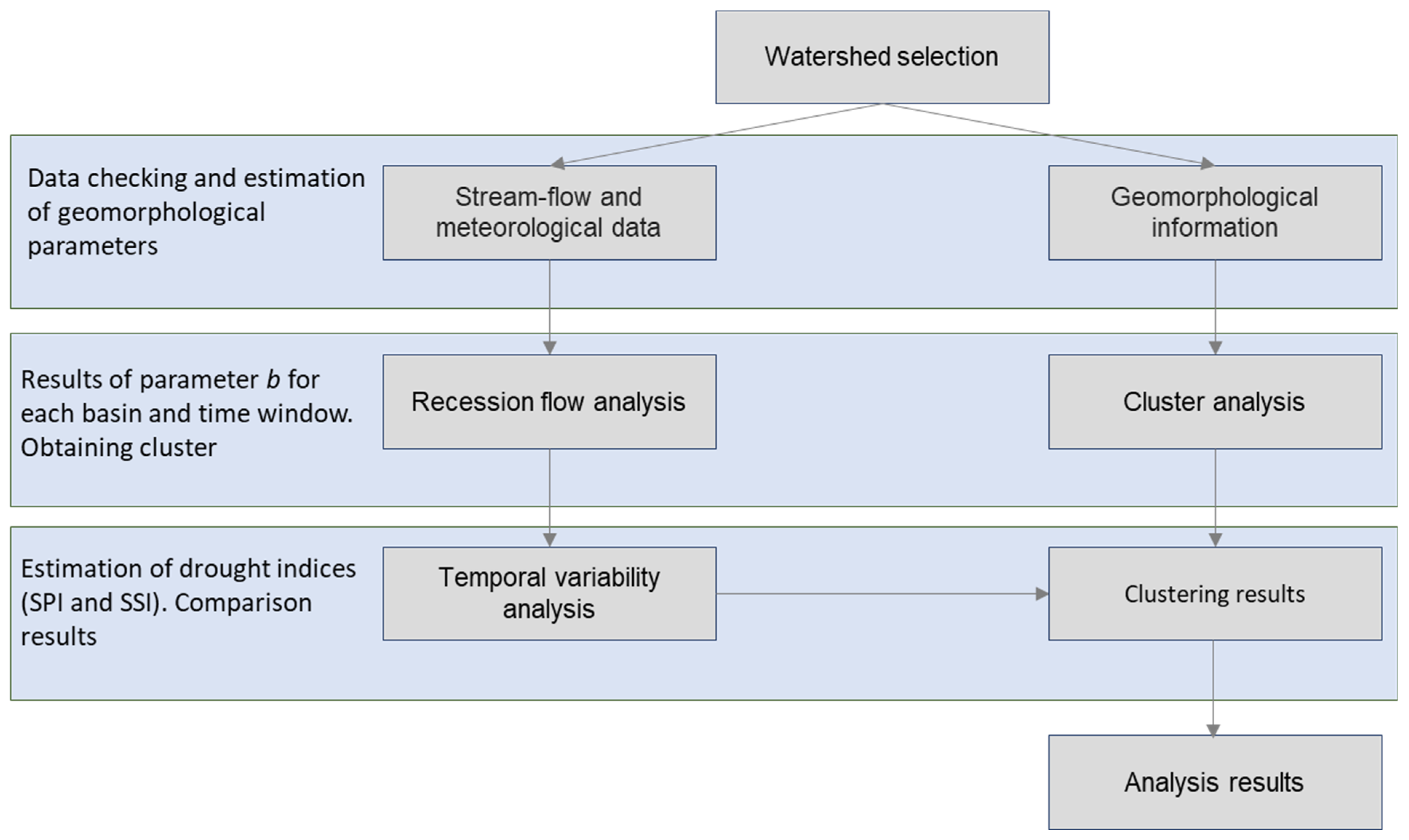
2. Materials and Methods

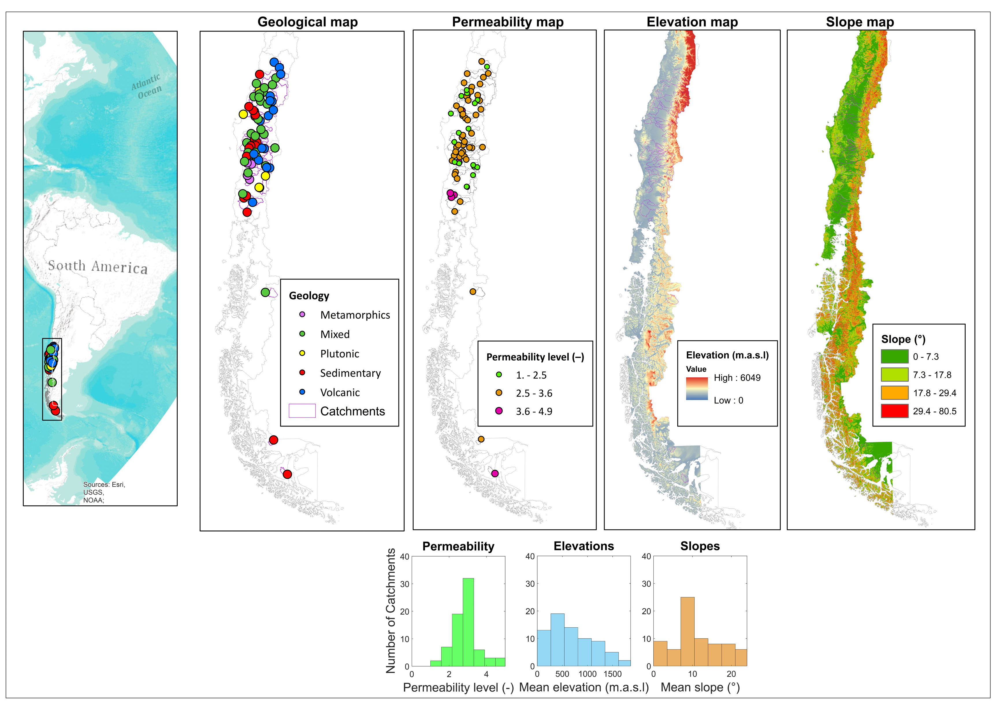
2.1. Study Area and Data

The study area includes 72 drainage basins located in south central Chile, between latitudes 30°00″ and 56°30′ S (Figure 1). To rule out the influence of anthropogenic effects (for example, of dams, canals, etc.), basins without human alterations or minimally affected via land-use change or artificial storage were selected for the analyses.
In general, the selected basins in the central zone (latitudes ~30–40° S) present a Mediterranean climate, with precipitation ranging between 100 and 3000 mm/year. The basins located in the austral zone of Chile (latitudes ~40–56°30′ S) present a wet climate, with precipitation ranging from 2000 to 4000 mm/year [31,32].
Continuous tectonic activity formed the existing physiographic (Coastal Range, Central Valley, and Andes Mountains) and geological characteristics along the length of Chile [33]. These characteristics determine the hydrological behavior and hydrogeological and geomorphological properties of the drainage basins in the study area. The basins present hydrological regimes (pluvial and pluvio-nival) regulated by physiographic and climate characteristics. The pluvial basins present precipitation seasonality, while the pluvio-nival basins present interannual variability that is controlled via precipitation–accumulation–snowmelt processes in the Andes Mountains [34]. The geological map of Chile [33] shows that basins present spatial variability of geological (volcanic, plutonic, metamorphic, sedimentary, and mixed) formations, with different characteristics (fractures, porosity, permeability, etc.) that determine the capacity of a basin to conduct and transmit water, allowing water infiltration, storage, and discharge [35]. The studied basins are monitored on the western slope of the Andes Mountains, the Central Valley, and the Coastal Range. Given their geographic location and orientation (east to west), the basins present spatial variation in geomorphological characteristics, with areas between 100 and 20,515 km2, mean elevations from above 100 m.a.s.l. to 1860 m.a.s.l., and mean slopes between 1 and 25°.
Using the geological map of Chile, which has a resolution of 1:1,000,000 (SERNAGEOMIN [33]), a geological classification of the 72 studied basins was carried out, considering the proportion (%) of geological formations present in each studied basin. Based on the predominant geological formation (that covers more than 50% of the basin), the basins were classified as sedimentary, volcanic, plutonic, or metamorphic. The basins that did not present a predominant geological formation were classified as mixed. In accordance with the classification, 20 basins present a predominant sedimentary geology (SG), 17 a volcanic geology (VG), 4 a plutonic geology (PG), 5 a metamorphic geology (MG), and 26 a mixed geology (MiG). In addition, based on the geological formations and the drainage network of each basin, a qualitative assessment of the average degree of permeability (kp) of the studied basins was carried out. They were assigned a permeability value according to the type of geological formation present in each stream/river section of the basin drainage network. The permeability value assigned to each stream/river section was then averaged to obtain the representative value (degree) of permeability for the entire contributing catchment of the main river section (until obtaining a value for the entire basin). A value of 5.0 was assigned to formations with greater permeability (e.g., fractured volcanic geology) and 1.0 to formations with less permeability (e.g., plutonic geology). Figure 1 presents the location of the study area, along with some important characteristics of each studied basin (geological classification, mean elevation, mean slope, and degree of permeability). In addition, Appendix A presents a table with the main characteristics of the studied basins.
The recession flow analysis used the mean daily flows obtained from the Catchment Attributes and Meteorology for Large Sample Studies—Chile Dataset (CAMELS-CL), presented by Alvarez-Garreton et al. [32], which includes hydrometeorological information from all of Chile. In all basins, the mean daily flow records from the 1990–2019 period were selected. The information obtained from the CAMELS-CL database can be used directly without applying data processing methods.

2.2. Recession Flow Analysis

Mean daily flow data were used for the analysis discarding the months associated with the snowmelt periods (October–December) of each year of records in order to represent only periods in which river baseflow is generated via groundwater release.
Recession events were identified based on the hydrograph of each basin when dQ/dt was less than zero for at least 5 consecutive days until dQ/dt was greater than zero. The start of the recession events was defined as 1 day after the maximum flow to avoid the influence associated with precipitation–runoff processes. The end of the recession events was when dQ/dt was positive in the hydrographs [28,36].
The methodology consisted of graphing the logarithm of the rate of change in flow (dQ/dt) against the logarithm of the average discharge ( Q i + Q i 1 )/2) during the same period. The rate of change dQ/dt was calculated using the exponential time step (ETS) method proposed by Roques et al. [36], which is programmed in MATLAB with open-source code, allowing the adaptations and optimizations necessary to achieve the objective of this study.

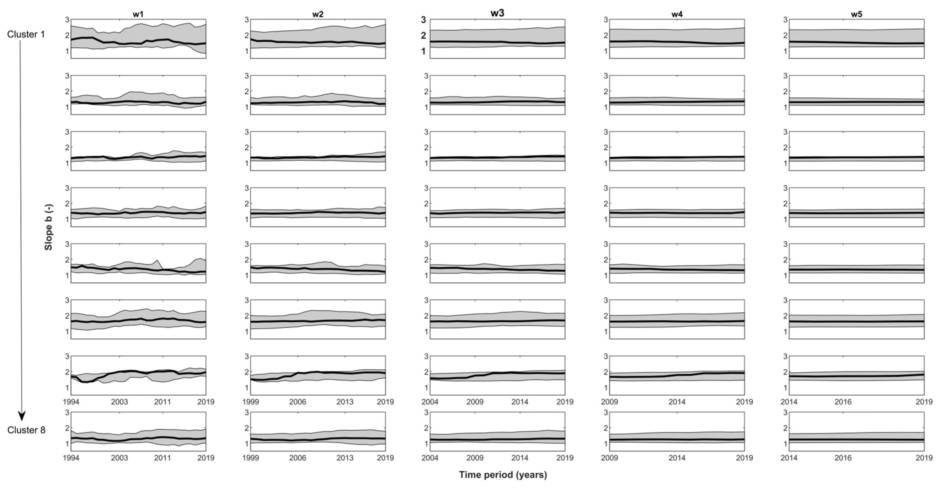
2.3. Temporal Variability in Recession Flows

A temporal analysis of clustered recession events (point cloud) was carried out to analyze the variability of parameter b over time, as well as to identify a minimum length of records needed to perform an adequate recession flow analysis. To this end, five moving (time) windows of 5 years (w1), 10 years (w2), 15 years (w3), 20 years (w4), and 25 years (w5) were analyzed. The time windows were selected with the aim of determining the behavior of the average S-Q process of each basin at different time scales, covering seasonality and long-term processes such as climate variability.
Recession data on a log–log plot can be analyzed using 3 lower envelopes (3 slopes) under the point cloud [7]. Given that the exact position of the envelopes is uncertain [37], a clustered data (bin) regression was carried out to plot a central line using the recession data. Slope b of the clustered data provides information on the average recession behavior of the entire basin, which aids in the identification of the average behavior of groundwater storage–runoff processes [13]. The recession data were grouped into data bins in accordance with the methodology used by Kirchner [9]. To obtain the bins, the recession flows were put in descending order, and equal intervals with 5% of the data were obtained. In each interval, an average of log (dQ/dt) and log (Q) was calculated, and, using the least squares method, the value of slope b was determined, which represents the average storage–release behavior of the basin.
To link the temporal behavior of recession slope b with drought events, the Standardized Precipitation Index (SPI) and Standardized Streamflow Index (SSI) were estimated using the mean monthly precipitation and flow records of each basin. These indices detect extreme (dry and wet) periods in the long term, allowing the analysis of drought periods.
To obtain the indices, a time scale (i = 3, 6, 12, 24, 36, or 48 months) must be chosen, where for each month, a cumulative value is determined considering the previous i months. A probability distribution is fitted to the obtained sets, which are then transformed into a standard normal distribution with a mean of 0 and a variance of 1. Both indices (SPI and SSI) are estimated considering a time scale of 48 months, as changes in groundwater storage respond to long-term changes in precipitation/runoff. The intensity of dry or wet events according to SPI and SSI values is shown in Table 1.

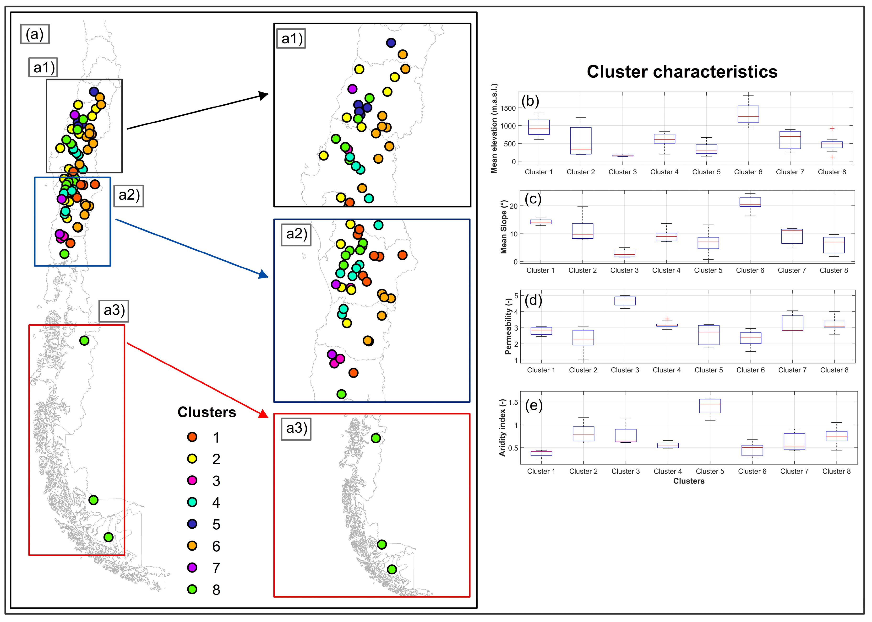
2.4. Cluster Analysis

To analyze spatial variability patterns and generate groups of basins with similar characteristics, a cluster (C) analysis was carried out. Clusters were obtained using the principal component analysis (PCA) and K-means methods, both programmed in MATLAB. The PCA method delivers the coefficients of the principal components, the score values of each object, and the variance values for each principal component. The principal components are selected as clustering axes on an XY graph.
The final clustering was performed via K-means. This method requires the number of groups (K) as an input parameter to cluster the data. Based on the number of groups, the algorithm randomly assigns K centroids that represent the center of each cluster. Next, the distances between each centroid and the data (or observations) are calculated, assigning all observations to the nearest cluster (nearest centroid). Subsequently, the centroids are recalculated, generating a new data assignment (data nearest a new centroid). The process is repeated iteratively until the assignment does not change (the centroid of each cluster stabilizes).
The squared Euclidian distance was used for the analysis, and the initial positions of each centroid were selected based on n random observations of the considered characteristics. In total, 8 groups were obtained using degree of permeability, mean slope, and aridity index as clustering characteristics. The aridity index was obtained based on the relationship between the mean annual precipitation and evapotranspiration of each basin. Figure 2 shows a flowchart that summarizes the methodology used in this study.

3. Results and Discussion

3.1. Basin-Scale Spatial Distribution of Characteristics

Figure 3 presents the eight clusters obtained via cluster analysis. In addition, the figure shows the hydrogeological, morphological, and climate characteristics of the basins for each group (mean elevation, mean slope, degree of permeability, and aridity index). In accordance with the classification, the basins that compose clusters C1 and C6 are located in Andes Mountains and foothills (Figure 3a), with mean elevations from 650 to 1900 m.a.s.l. (Figure 3b). These basins present steep topographies, with slopes over 13°. They also present medium to low permeability that is associated with the predominant geological characteristics of the basins that compose the groups (volcanic, plutonic, and mixed). Finally, these basins present aridity indices below 1 (Figure 3e), corresponding to their geographic location (Andes Mountains), where precipitation is greater than evapotranspiration [32,40].
Meanwhile, C3 and C5 are composed of basins monitored in the Central Valley (Figure 3a), with mean elevations below 600 m.a.s.l. (Figure 3b). In general, the basins present flat topographies, with slopes between 0.7 and 7°, except for one basin that presents a slope of ~13°. The degree of permeability of these basins is variable (low, medium, and high), which is associated with their predominantly plutonic (low permeability), volcanic and mixed (medium permeability), and sedimentary (high permeability) geological characteristics.
Cluster 7 is composed of basins monitored in the Coastal Range (Figure 3a), with mean elevations between 200 and 800 m.a.s.l. and slopes between 4 and 11° (Figure 3b,c). The degree of permeability of these basins is medium–high, associated with sedimentary to mixed characteristics.
Clusters C2, C4, and C8 are composed of basins monitored in the Andes Mountains, Central Valley, and Coastal Range (Figure 3a), a broad group of basins with heterogeneous characteristics. These basins present mean elevations between 100 and 900 m.a.s.l., mean slopes between 2 and 14°, and low, medium, and high degrees of permeability associated with their different geological characteristics (plutonic, metamorphic, sedimentary, and mixed).

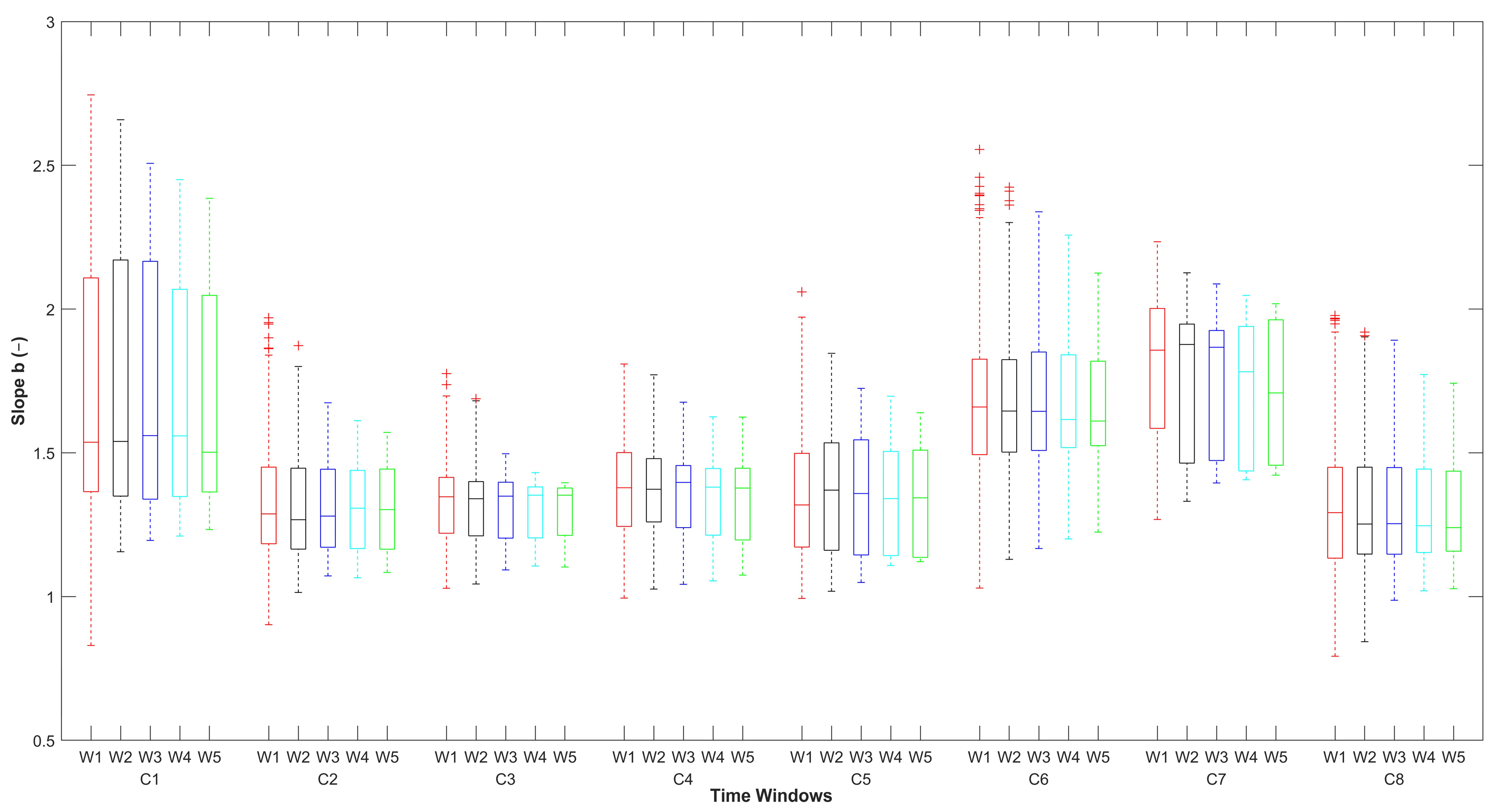
3.2. Temporal Variability of Recession Parameter b

Figure 4 shows the mean temporal variation of recession parameter b for each group of basins (clusters in rows) and moving time window (w1, w2, w3, w4, and w5 in columns), while Figure 5 shows the variability of b for each cluster and moving window w. In general, it is observed that slope b presents significant variability over time in all the basin clusters for the analyzed time windows (w1, w2, w3, w4, and w5); however, as the time window increases (w greater than 10 years), the variability of slope b tends to be more stable. This indicates that with greater temporal aggregation of recession data, interannual variability is attenuated; therefore, with a greater temporal aggregation of recession data, it would be possible to detect changes in the rate of S-Q changes (represented by b) amid dry or wet periods (climate variability).
In addition, Figure 4 shows that, despite the variability presented, b maintains an upward or downward trend in the five moving windows used for the analysis (e.g., C1, C3, C5, and C7; see Figure 4). This could indicate that independent of the moving time window length or time period of analysis, the S-Q behavior trend is strongly influenced by the geological, topographical, and hydroclimatic characteristics in the studied basins. These basins were selected based on their predominant geology; however, they may present other geological formations to a lesser extent that could influence the hydrogeological conditions (permeability, underground connections between basins) and, therefore, the behavior of the groundwater storage–release process represented by slope b. In addition, the physiographic characteristics of the zone where the basins are located may present topographic variability and, thus, variability in terrain slopes, characteristics that also likely influence S-Q behavior [41]. This observed behavior is consistent with the findings of Li and Ameli [42], who mention that terrain slope (topography) is one of the main drivers in subsoil storage and release processes.
Meanwhile, Figure 5 shows that the variability of parameter b is greater in the basins of clusters C1 and C6, which are located in the Andes Mountains and have a greater proportion of fractured volcanic and mixed geology and steeply sloped topography. By contrast, basins located in the Central Valley (in groups C3 and C5), with sedimentary geology and flat slopes, present less variation in slope b. This indicates that the basins with volcanic and mixed geology likely present complex aquifer structures, possibly with significant fractures or faults that control the storage and flow of groundwater [43]. The complexity of these aquifer systems with volcanic and mixed geology leads to variable groundwater storage and release behavior, represented by the high variability of slope b in these basins.

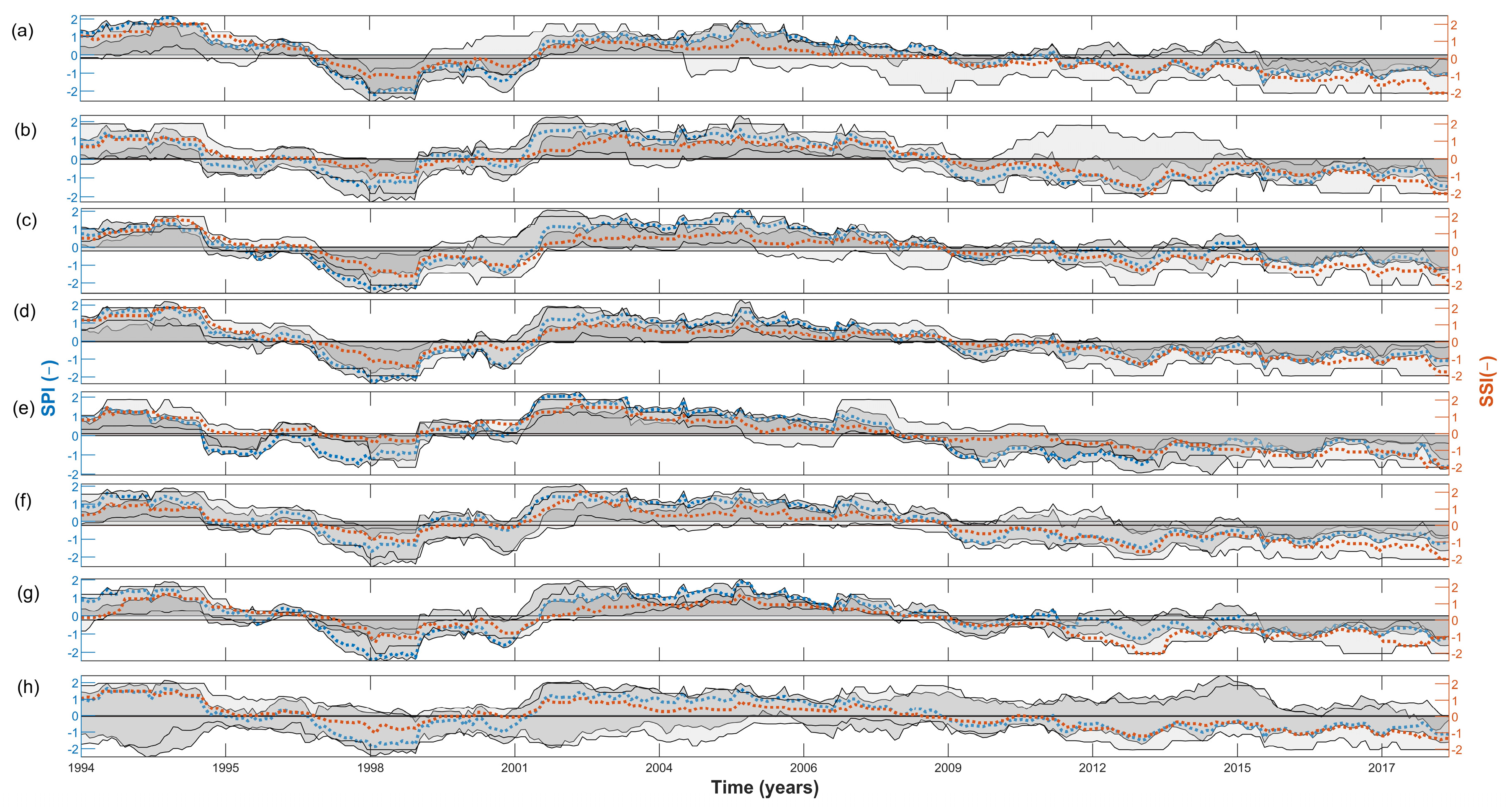
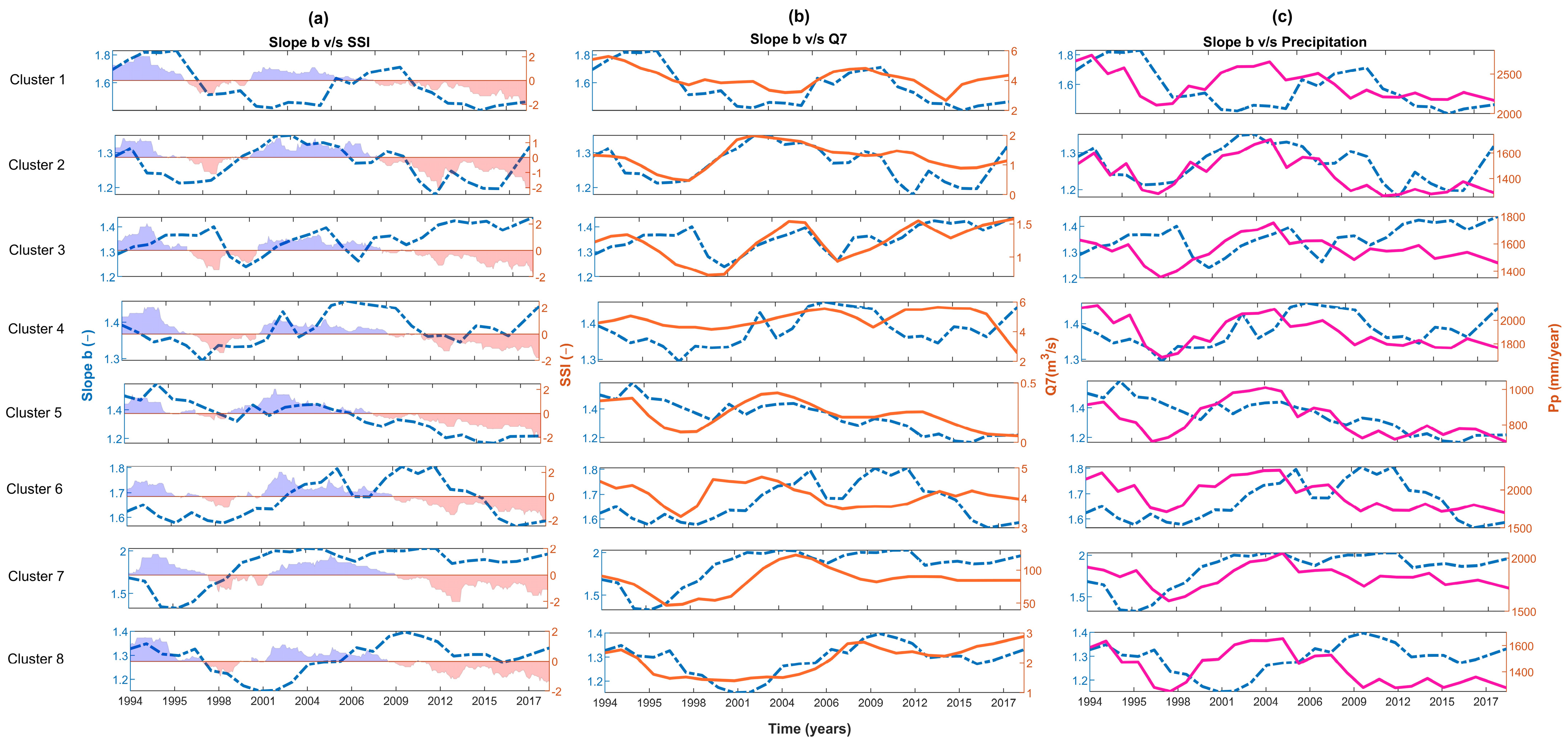
3.3. Influence of Climate Behavior on S-Q Behavior

Figure 6 shows the comparison between the mean SPI and SSI values of each study group, considering a time scale of 48 months. In general, it is observed that the two indices present similar temporal behavior, with dry and wet periods identified, only differing slightly in magnitude. In most of the studied basins, a first dry period (SPI o SSI < −1) is observed, spanning from 1998 to early 2000 (see Figure 6). A long second period with moderate and severe droughts is observed between 2010 and 2019, a period that locally has been called a megadrought [44]. In contrast, it is observed that the wet periods (SPI o SSI > 1) occurred in the years 1994–1997 and 2000–2008.
Figure 7 shows the temporal variation of the 50th percentile of slope b for window w1 (5 years) of each basin group with the 50th percentile of the temporal variation of the Standardized Streamflow Index (SSI), the mean annual minimum 7-day flow (Q7), and mean annual precipitation (Pp). In general, it is observed that recession parameter b increases in wet periods and decreases in dry periods (see Figure 7a), except in Cluster 7, which presents variations independent of dry or wet periods. The increase in slope b in wet periods is likely associated with rapid groundwater storage and release processes caused by the greater recharge and increase in groundwater levels due to the increase in annual precipitation in these periods (see Figure 7c). In contrast, the decrease in recession parameter b in dry periods is likely associated with the slowing of the groundwater storage and release process and, thus, decreased aquifer storage due to the emptying of the aquifer as a result of the scarcity of rainfall. Therefore, a decrease in the contribution of water from the aquifer to the baseflow due to lower recharge would result in a decrease in recession slope b [10].
The observed variability of slope b in wet and dry periods does not present a clear pattern in the clusters, which could be because the dry periods between 1990 and 2010 are not prolonged; therefore, the storage that is contributing to the flow is dynamic [5,9,45] or active storage [46]. Dynamic storage is defined as the fraction of the total storage of the aquifer that directly contributes to the basin flow [5,19,47]. Thus, in limited drought periods, the variability of slope b (decrease or increase) could be an effect of the contribution of the dynamic storage of the aquifer, which may present high variability among basins [5].
In general, in the 2010–2019 period, it is observed that recession parameter b presents slight variations in most of the basin groups, except for C3, in which b presents a relatively upward trend. The basins in this group are located in the Central Valley of southern Chile and have sequences of sedimentary and metamorphic geology and moderate slopes (Figure 3). The rise of slope b is consistent with the increase in flow, which also presents a slightly upward trend (Q7, see Figure 7b) between 2010 and 2019. This could be because these basins are likely formed by shallow soils (alluvial rocks and pyroclasts, SERNAGEOMIN [30]), which, despite the precipitation deficit, would maintain saturated conditions (Figure 7a,c). In this regard, Balocchi et al. [48] mention that the recession coefficient depends on the degree of saturation of the basin before the recession period.
It is also observed that starting in 2016, there is an increase in slope b in the groups. This increase in b is moderate in some groups composed mainly of basins with a volcanic and sedimentary predominance (C1, C3, C5, C6, and C7, Figure 7), while in groups composed of basins with a greater mixed and sedimentary predominance, the increase in b is more progressive (C2, C4, and C8). This increase in b is not consistent with precipitation, as between 2016 and 2019, precipitation tended to decrease in all basin groups; however, the flows increased (C1, C3, and C8) or stabilized to a relatively constant flow (C2, C5, C6, and C7). The basins of group C4 presented a behavior that differed from that of the other groups, with decreasing flows between 2016 and 2019. The increase in recession parameter b could be associated with the fact that in a prolonged period of dry years (>7 years), dynamic storage tends to affect discharge, beginning to contribute deep storage (also called “indirect storage” by Dralle et al. [46]) and mobile storage (named by Staudinger et al. [47]) to runoff generation in the studied basins. Deep storage can be defined as the part of the total storage that has remained in the aquifer for a long time. Therefore, deep storage participates in flow contribution to the basin, possibly with water associated with long-term recharge [47].
The variability of recession coefficient b indicates changes in S-Q behavior; therefore, it could be used as an indicator of basin sensitivity to climate variability. To corroborate that after a certain number of years (>7 years), dynamic storage ceases and deep storage begins to act would require a greater length of drought period precipitation data. Nonetheless, the analysis of the temporal variation of the recession parameter shows that in a prolonged drought period, dynamic storage can act initially, followed by deep storage. Understanding and identifying this S-Q dynamic could contribute to improving low-flow predictions in dry periods.

3.4. Implications of the Study and Future Research

Recession parameter b has been used to evaluate the behavior of groundwater storage and its association with basin-scale characteristics [10,11,49,50]. In this regard, variability of b related to the heterogeneity of the hydrogeological and geomorphological characteristics of a basin has been found in some studies, e.g., [3,21,46]. In this study, we complemented these findings by analyzing the variability of parameter b at different time scales. We found that the variability of b is also influenced by climatic variability since b tends to decrease in dry periods and increase in wet periods. The observed behavior of b is essential for identifying the sensitivity of a basin to dry periods since the rainfall decrease in dry periods impacts groundwater recharge [51], which directly affects groundwater storage.
Future research in this line could focus on the connections among climate, basin storage state, and recession, as well as the connection with physical characteristics of basins (i.e., geology and morphology). In addition, studying the temporal variability of groundwater storage can contribute to improving the evaluation and prediction of groundwater behavior under climate change scenarios.

4. Conclusions

The present study was focused on the analysis of the temporal variability of recession parameter b, which represents groundwater storage and release behavior, and how this variability is related to basin characteristics and climate variability. In general, it was found that in wet periods, the recession parameter tends to increase (fast drainage process), while in dry periods, the recession parameter tends to decrease (slow drainage processes).
The temporal variation (increase and/or decrease) of the slope is associated with the contribution of the dynamic storage of the aquifer to the river flow, which responds to periods of higher or lower precipitation to maintain river baseflow. In addition, in prolonged dry periods, it was found that starting in year 7, the recession slope tended to increase in most studied basins, maintaining river baseflow. Preliminarily, the results suggest that in prolonged dry periods, the “dynamic storage” of the aquifer makes a primary contribution before giving way to deep storage contribution to river flow; however, this analysis must be deepened with a greater analyzed data length to allow greater certainty on this matter.
In general, the results suggest that the variability of recession coefficient b indicates changes in S-Q behavior, making it suitable for use as an indicator of basin sensitivity to climate variability. Therefore, a temporal analysis of b could be a valuable tool to improve the prediction of low flows.

Author Contributions

Investigation, V.P.; Conceptualization, V.P. and E.M.; Methodology, V.P. and E.M.; Formal analysis, V.P., E.M., J.L.A., and Y.M.; Writing—review and editing, V.P., E.M., J.L.A., and Y.M. All authors have read and agreed to the published version of the manuscript.

Funding

This research was funded by the ANID/FONDECYT/3220246 project.

Data Availability Statement

In this study, publicly available datasets were analyzed. These data can be found here: https://camels.cr2.cl/ (accessed on 15 March 2023).

Acknowledgments

The authors thank the General Water Directorate for providing the data used to develop this study, the Center for Climate and Resilience Research (CR)2 for providing data through its https://camels.cr2.cl/ platform (accessed on 20 April 2022), ANID/FONDECYT/3220246, the CRHIAM Water Center ANID/FONDAP/15130015 and to Universidad Católica de la Santísima Concepción FAA 2023. The authors also thank to Clement Roques, David Rupp, and John Selker for providing the MATLAB code base used in this study.

Conflicts of Interest

The authors declare no conflict of interest.

Appendix A

Table A1. Information on the 72 basins analyzed in this study.
Gauge NameGauge Latitude (°)Gauge Longitude (°)Area (km2)Mean Elevation (m)Mean Slope (°)Geologic ClassDegree of Permeability (-)Aridity Index (-)
Estero Zamorano En Puente El Niche−34.4−71.2102367213.2MiG3.11.6
Rio Quepe En Quepe−38.9−72.616665067.3MiG3.20.5
Rio Cauquenes En El Arrayan−36.0−72.46223088.3MiG1.81.2
Rio Purapel En Sauzal−35.8−72.14042947.0PG1.71.5
Rio Andalien Camino A Penco−36.8−73.07502107.7PG1.01.0
Rio Lumaco En Lumaco−38.2−72.98533419.7MiG1.71.0
Estero Curipeumo En Lo Hernandez−36.0−72.02171370.7SG3.21.6
Rio Loncomilla En Bodega−35.8−71.870793987.1MiG2.71.1
Rio Mininco En Longitudinal−37.9−72.44404503.3SG3.00.6
Rio Malleco En Collipulli−38.0−72.441580113.8MiG3.00.4
Rio Traiguen En Victoria−38.2−72.3945132.1SG3.00.6
Rio Dumo En Santa Ana−38.2−72.33934852.4SG3.00.7
Rio Quino En Longitudinal−38.3−72.42775813.6SG3.00.5
Estero Chufquen En Chufquen−38.3−72.78544292.7SG3.00.7
Rio Quillen En Galvarino−38.4−72.87102853.7SG3.10.9
Rio Larqui En Santa Cruz De Cuca−36.7−72.46361501.7SG5.01.1
Rio Lirquen En Cerro El Padre−37.8−71.910366813.7MiG3.50.5
Rio Donguil En Gorbea−39.1−72.77702065.1MG4.20.6
Rio Negro En Chahuilco−40.7−73.222801523.2SG4.60.6
Rio Damas En Tacamo−40.6−73.14671321.6SG4.80.7
Rio Negro En Las Lomas−41.4−73.12531181.8SG3.60.4
Rio Cholchol En Cholchol−38.6−72.850483427.0MiG2.60.8
Rio Puyehue En Quitratue−39.2−72.71532008.9MG2.20.6
Rio Mahuidanche En Santa Ana−39.1−72.938418910.2MG2.20.6
Rio Collileufu En Los Lagos−39.9−72.86261978.1MG2.50.7
Rio Inaque En Mafil−39.7−73.05392048.6MG2.90.6
Rio Cauquenes En Desembocadura−35.9−72.116372465.9MiG2.01.3
Rio Loncomilla En Las Brisas−35.6−71.899244898.7MiG2.81.0
Rio Vergara En Tijeral−37.7−72.625373758.1MiG2.20.8
Rio Muco En Puente Muco−38.6−72.46505377.1MiG3.10.6
Rio Cruces En Rucaco−39.6−72.918032827.9MiG3.40.5
Rio Longavi En El Castillo−36.3−71.3467156424.4VG2.70.5
Rio Achibueno En La Recova−36.0−71.4894132923.0VG2.90.6
Rio Itata En Cholguan−37.2−72.186083412.1VG3.10.6
Rio Diguillin En San Lorenzo (Atacalco)−36.9−71.6204151122.8VG2.70.4
Rio Coihueco Antes Junta Pichicope−40.9−72.731360814.1VG3.00.3
Rio Perquilauquen En Gniquen−36.2−72.0120964711.2MiG2.60.7
Rio Perquilauquen En Quella−36.1−72.116875058.6MiG2.90.9
Rio Itata En General Cruz−36.9−72.416626137.9SG3.20.7
Rio Itata En Trilaleo−37.1−72.2114875210.2MiG3.20.7
Rio Diguillin En Longitudinal−36.9−72.3130078510.1SG3.20.6
Rio Itata En Balsa Nueva Aldea−36.7−72.545105047.0SG3.30.8
Rio Itata En Coelemu−36.5−72.710,4056169.0SG3.30.8
Rio Renaico En Longitudinal−37.9−72.468883316.0MiG2.60.4
Rio Huichahue En Faja 24000−38.9−72.334860512.9MiG3.10.4
Rio Cautin En Almagro−38.8−72.955475537.4SG3.10.5
Estero Upeo En Upeo−35.2−71.1367119719.8MiG2.90.8
Rio Mataquito En Licanten−35.0−72.05700123015.2SG3.00.9
Rio Perquilauquen En San Manuel−36.4−71.6502110020.5MiG2.00.5
Rio Longavi En La Quiriquina−36.2−71.5669140123.0VG2.50.5
Rio Lircay En Puente Las Rastras−35.5−71.3382105214.4MiG3.10.6
Rio Duqueco En Villucura−37.6−72.0818102316.4MiG2.30.5
Rio Tolten En Teodoro Schmidt−39.0−73.1792770211.1MiG2.80.4
Rio Rahue En Forrahue−40.5−73.356032344.9MiG4.10.5
Rio Ñirehuao En Villa Mañihuales−45.2−72.119979269.7MiG3.51.1
Rio Claro En El Valle−34.7−70.9349160520.0VG2.50.7
Rio Claro En Los QueñEs−35.0−70.8354185723.8VG2.70.6
Rio Sauces Antes Junta Con Ñuble−36.7−71.3607168322.8VG2.90.6
Rio Blanco En Curacautin−38.5−71.9171129713.4VG2.90.3
Rio Cautin En Rari-Ruca−38.4−72.01306112513.5VG2.90.4
Rio Allipen En Los Laureles−39.0−72.21675102114.7VG2.50.4
Rio Nilahue En Mayay−40.3−72.230991414.5VG2.50.3
Rio Liucura En Liucura−39.3−71.8349103819.4MiG1.90.4
Rio Liquine En Liquine−39.7−71.8368112219.8PG1.50.3
Rio Calcurrupe En Desembocadura−40.3−72.3172693620.5PG1.60.3
Rio San Juan En Desembocadura−53.7−71.08643428.8SG4.00.8
Rio Maule En Forel−35.4−72.220,51589011.8MiG2.80.9
Rio Lonquimay Antes Junta Rio Bio Bio−38.4−71.2467135915.6MiG2.60.4
Rio Cautin En Cajon−38.7−72.527567639.2VG3.00.5
Rio Trancura En Curarrehue−39.4−71.6357119520.2VG2.30.3
Rio Trancura Antes Rio Llafenco−39.3−71.81379114718.3VG2.40.3
Rio Rubens En Ruta N 9−52.0−71.95044157.4SG3.50.7
Notes: SG: sedimentary; VG: volcanic; PG: plutonic, MG: metamorphic and MiG: mixed.

References

  1. Condon, L.E.; Atchley, A.L.; Maxwell, R.M. Evapotranspiration depletes groundwater under warming over the contiguous United States. Nat. Commun. 2020, 11, 873. [Google Scholar] [CrossRef] [PubMed] [Green Version]
  2. Patnaik, S.; Biswal, B.; Kumar, D.N.; Bellie Sivakumar, B. Regional variation of recession flow power-law exponent. Hydrol. Process. 2018, 32, 866–872. [Google Scholar] [CrossRef]
  3. Jachens, E.R.; Rupp, D.E.; Roques, C.; Selker, J.S. Recession analysis revisited: Impacts of climate on parameter estimation. Hydrol. Earth Syst. Sci. 2020, 24, 1159–1170. [Google Scholar] [CrossRef] [Green Version]
  4. Shao, C.; Liu, Y. Analysis of Groundwater Storage Changes and Influencing Factors in China Based on GRACE Data. Atmosphere 2023, 14, 250. [Google Scholar] [CrossRef]
  5. Karimi, S.; Seibert, S.; Laudon, H. Evaluating the effects of alternative model structures on dynamic storage simulation in heterogeneous boreal catchments. Hydrol. Res. 2022, 53, 562–583. [Google Scholar] [CrossRef]
  6. Adams, K.H.; Reager, J.T.; Rosen, P.; Wiese, D.N.; Farr, T.G.; Rao, S.; Haines, B.J.; Argus, D.F.; Liu, Z.; Smith, R.; et al. Remote sensing of groundwater: Current capabilities and future directions. Water Resour. Res. 2022, 58, e2022WR032219. [Google Scholar] [CrossRef]
  7. Brutsaert, W.; Nieber, J.L. Regionalized drought flow hydrographs from a mature glaciated plateau. Water Resour. Res. 1977, 13, 637–643. [Google Scholar] [CrossRef]
  8. Tallaksen, L. A review of baseflow recession analysis. J. Hydrol. 1995, 65, 349–370. [Google Scholar] [CrossRef]
  9. Kirchner, J.W. Catchments as simple dynamical systems: Catchment characterization, rainfall-runoff modeling, and doing hydrology backward. Water Resour. Res. 2009, 45, W02429. [Google Scholar] [CrossRef] [Green Version]
  10. Biswal, B.; Marani, M. Universal recession curves and their geomorphological interpretation. Adv. Water Resour. 2014, 65, 34–42. [Google Scholar] [CrossRef]
  11. Parra, V.; Arumí, J.L.; Muñoz, E.I. Characterization of the Groundwater Storage Systems of South-Central Chile: An Approach Based on Recession Flow Analysis. Water 2019, 11, 1506. [Google Scholar] [CrossRef] [Green Version]
  12. Huang, C.; Yeh, H. Impact of climate and NDVI changes on catchment storage–discharge dynamics in southern Taiwan. Hydrol. Sci. J. 2022, 67, 1834–1845. [Google Scholar] [CrossRef]
  13. Mendoza, G.F.; Steenhuis, T.S.; Walter, M.T.; Parlange, J.Y. Estimating basin-wide hydraulic parameters of a semi-arid mountainous watershed by recession-flow analysis. J. Hydrol. 2003, 279, 57–69. [Google Scholar] [CrossRef]
  14. Oyarzún, R.; Godoy, R.; Núñez, J.; Fairley, J.P.; Oyarzún, J.; Maturana, H.; Freixas, G. Recession flow analysis as a suitable tool for hydrogeological parameter determination in steep, arid basins. J. Arid. Environ. 2014, 105, 1–11. [Google Scholar] [CrossRef]
  15. Brutsaert, W. Long-term groundwater storage trends estimated from streamflow records: Climatic perspective. Water Resour. Res. 2008, 44, W02409. [Google Scholar] [CrossRef]
  16. Lin, K.T.; Yeh, H.F. Baseflow recession characterization and groundwater storage trends in northern Taiwan. Hydrol. Res. 2017, 48, 1745–1756. [Google Scholar] [CrossRef]
  17. Yan, H.; Hu, H.; Liu, Y.; Tudaji, M.; Yang, T.; Wei, Z.; Chen, L.; Ali Khan, M.Y.; Chen, Z. Characterizing the groundwater storage–discharge relationship of small catchments in China. Hydrol. Res. 2022, 53, 782–794. [Google Scholar] [CrossRef]
  18. Lin, L.; Gao, M.; Liu, J.; Wang, J.; Wang, S.; Chen, X.; Liu, H. Understanding the effects of climate warming on streamflow and active groundwater storage in an alpine catchment: The upper Lhasa River. Hydrol. Earth Syst. Sci. 2020, 24, 1145–1157. [Google Scholar] [CrossRef] [Green Version]
  19. Buttle, J.M. Dynamic storage: A potential metric of inter-basin differences in storage properties. Hydrol. Process. 2016, 30, 4644–4653. [Google Scholar] [CrossRef]
  20. Fan, Y.; Clark, M.; Lawrence, D.; Swenson, S.; Band, L.E.; Brantley, S.; Brooks, P.; Dietrich, W.; Flores, A.; Grant, G.; et al. Hillslope Hydrology in Global Change Research and Earth System Modeling. Water Resour. Res. 2019, 55, 1737–1772. [Google Scholar] [CrossRef] [Green Version]
  21. Shaw, S.B.; Riha, S.J. Examining individual recession events instead of a data cloud: Using a modified interpretation of dQ/dt -Q streamflow recession in glaciated watersheds to better inform models of low flow. J. Hydrol. 2012, 434, 46–54. [Google Scholar] [CrossRef]
  22. Sánchez-Murillo, R.; Brooks, E.S.; Elliot, W.J.; Gazel, E.; Boll, J. Baseflow recession analysis in the in land Pacific Northwest of the United States. Hydrogeol. J. 2015, 23, 287–303. [Google Scholar] [CrossRef]
  23. Brutsaert, W.; Lopez, J.P. Basin-scale geohydrologic drought Flow features of riparian aquifers in the southern Great Plains. Water Resour. Res. 1998, 34, 233–240. [Google Scholar] [CrossRef]
  24. Ceola, S.; Botter, G.; Bertuzzo, E.; Porporato, A.; Rodriguez-Iturbe, I.; Rinaldo, A. Comparative study of ecohydrological streamflow probability distributions. Water Resour. Res. 2010, 46, W09502. [Google Scholar] [CrossRef] [Green Version]
  25. Ye, S.; Li, H.; Huang, M.; Ali, M.; Leng, G.; Leung, L.R.; Sivapalan, M. Regionalization of subsurface stormflow parameters of hydrologic models: Derivation from regional analysis of streamflow recession curves. J. Hydrol. 2014, 519, 670–682. [Google Scholar] [CrossRef] [Green Version]
  26. Chen, B.; Krajewski, W. Analysing individual recession events: Sensitivity of parameter determination to thecalculation procedure. Hydrol. Sci. J. 2016, 61, 2887–2901. [Google Scholar] [CrossRef] [Green Version]
  27. Santos, A.C.; Portela, M.M.; Rinaldo, A.; Schaefli, B. Estimation of streamflow recession parameters: New insights from an analytic streamflow distribution model. Hydrol. Process. 2019, 33, 1595–1609. [Google Scholar] [CrossRef]
  28. Jachens, E.R.; Roques, C.; Rupp, D.E.; Selker, J.S. Streamflow recession analysis using water height. Water Resour. Res. 2020, 56, e2020WR027091. [Google Scholar] [CrossRef]
  29. Huang, C.C.; Yeh, H.F. Evaluation of seasonal catchment dynamic storage components using an analytical streamflow duration curve model. Sustain. Environ. Res. 2022, 32, 49. [Google Scholar] [CrossRef]
  30. DGA. Atlas del Agua: Chile 2016; DGA: Santiago, Chile, 2016; Available online: https://snia.mop.gob.cl/repositoriodga/handle/20.500.13000/4371 (accessed on 16 March 2023).
  31. Garreaud, R.; Vuille, M.; Compagnucci, R.; Marengo, J. Present-day South American climate. Palaeogeogr. Palaeoclim. Palaeoecol. 2009, 281, 180–195. [Google Scholar] [CrossRef]
  32. Alvarez-Garreton, C.; Mendoza, P.A.; Boisier, J.P.; Addor, N.; Galleguillos, M.; Zambrano-Bigiarini, M.; Lara, A.; Puelma, C.; Cortes, G.; Garreaud, R.; et al. The CAMELS-CL dataset: Catchment attributes and meteorology for large sample studies—Chile dataset. Hydrol. Earth Syst. Sci. 2018, 22, 5817–5846. [Google Scholar] [CrossRef] [Green Version]
  33. Sernageomin. Mapa Geológico de Chile: Versión Digital; Servicio Nacional de Geología y Minería; Publicación Geológica Digital: Santiago, Chile, 2003.
  34. Rubio-Álvarez, E.; McPhee, J. Patterns of spatial and temporal variability in streamflow records in south central Chile in the period 1952–2003. Water Resour. Res. 2010, 46. [Google Scholar] [CrossRef]
  35. Voeckler, H.; Allen, D.M. Estimating regional-scale fractured bedrock hydraulic conductivity using discrete fracture network (DFN) modeling. Hydrogeol. J. 2012, 20, 1081–1100. [Google Scholar] [CrossRef]
  36. Roques, C.; Rupp, D.; Selker, J. Improved streamflow recession parameter estimation with attention to calculation of −dQ/dt. Adv. Water Resour. 2017, 108, 29–43. [Google Scholar] [CrossRef]
  37. Troch, P.A.; De Troch, F.P.; Brutsaert, W. Effective water-table depth to describe initial conditions prior to storm rainfall in humid regions. Water Resour. Res. 1993, 29, 427–434. [Google Scholar] [CrossRef]
  38. Wang, Y.; Duan, L.; Liu, T.; Li, J.; Feng, P. A Non-stationary Standardized Streamflow Index for hydrological drought using climate and human-induced indices as covariates. Sci. Total Environ. 2019, 699, 134278. [Google Scholar] [CrossRef]
  39. World Meteorological Organization. Standardized Precipitation Index User Guide. Available online: https://library.wmo.int/index.php?lvl=notice_display&id=13682 (accessed on 16 January 2023).
  40. Castro, L.; Gironás, J. Precipitation, Temperature and Evaporation. In Water Resources of Chile; Fernández, B., Gironás, J., Eds.; Springer: Cham, Switzerland, 2021; Volume 8. [Google Scholar] [CrossRef]
  41. Savenije, H.H. HESS opinions “topography driven conceptual modelling (FLEX-topo)”. Hydrol. Earth Syst. Sci. 2010, 14, 2681–2692. [Google Scholar] [CrossRef] [Green Version]
  42. Li, H.; Ameli, A. A statistical approach for identifying factors governing streamflow recession behaviour. Hydrol. Process. 2022, 36, e14718. [Google Scholar] [CrossRef]
  43. Fenta, M.C.; Anteneh, Z.L.; Szanyi, J.; Walker, D. Hydrogeological framework of the volcanic aquifers and groundwater quality in Dangila Town and the surrounding area, Northwest Ethiopia. Groundw. Sustain. Dev. 2020, 11, 100408. [Google Scholar] [CrossRef]
  44. Garreaud, R.D.; Boisier, J.P.; Rondanelli, R.; Montecinos, A.; Sepúlveda, H.H.; Veloso-Aguila, D. The Central Chile Mega Drought (2010–2018): A climate dynamics perspective. Int. J. Climatol. 2019, 40, 421–439. [Google Scholar] [CrossRef]
  45. McNamara, J.P.; Tetzlaff, D.; Bishop, K.; Soulsby, C.; Seyfried, M.; Peters, N.E.; Aulenbach, B.T.; Hooper, R. Storage as a metric of catchment comparison. Hydrol. Process. 2011, 25, 3364–3371. [Google Scholar] [CrossRef]
  46. Dralle, D.N.; Hahm, W.J.; Rempe, D.M.; Karst, N.J.; Thompson, S.E.; Dietrich, W.E. Quantification of the seasonal hillslope water storage that does not drive streamflow. Hydrol Process. 2018, 32, 1978–1992. [Google Scholar] [CrossRef]
  47. Staudinger, M.; Stoelzle, M.; Seeger, S.; Seibert, J.; Weiler, M.; Stahl, K. Catchment water storage variation with elevation. Hydrol. Process. 2017, 31, 2000–2015. [Google Scholar] [CrossRef]
  48. Balocchi, F.; Flores, N.; Arumí, J.L.; Iroumé, A.; White, D.A.; Silberstein, R.P.; Ramírez de Arellano, P. Comparison of streamflow recession between plantations and native forests in small catchments in Central-Southern Chile. Hydrol. Process. 2021, 35, e14182. [Google Scholar] [CrossRef]
  49. Mutzner, R.; Bertuzzo, E.; Tarolli, P.; Weijs, S.V.; Nicotina, L.; Ceola, S.; Rinaldo, A. Geomorphic signatures on brutsaert base flow recession analysis. Water Resour. Res. 2013, 49, 5462–5472. [Google Scholar] [CrossRef] [Green Version]
  50. Sharma, D.; Patnaik, S.; Biswal, B.; Reager, J.T. Characterization of Basin-Scale Dynamic Storage–Discharge Relationship Using Daily GRACE Based Storage Anomaly Data. Geosciences 2020, 10, 404. [Google Scholar] [CrossRef]
  51. Wu, W.Y.; Lo, M.H.; Wada, Y.; Famiglietti, J.S.; Reager, J.T.; Yeh, P.J.-F.; Ducharne, A.; Yang, Z. Divergent effects of climate change on future groundwater availability in key mid-latitude aquifers. Nat. Commun. 2020, 11, 3710. [Google Scholar] [CrossRef]
Figure 1. Locations of the drainage basins used in the study area and the predominant geology. In the geological map, the blue dots indicate basins with predominantly volcanic geology, the orange dots those with predominantly sedimentary geology, the green dots those with predominantly plutonic geology, the purple dots those with predominantly metamorphic geology, and the yellow dots those with mixed geology. In addition, some geomorphological (mean elevation and slope) and hydrogeological characteristics (degree of permeability) are shown.
Water 15 02503 g001
Figure 2. Diagram summarizing the methodology used in this study.
Water 15 02503 g002
Figure 3. Cluster results for the 72 basins, 1990–2020 period (a). The mean elevation (b), mean slope (c), degree of permeability (d), and aridity index (e) of each cluster are also shown. (a1a3) are the zooms of the squares of Figure 3a.
Water 15 02503 g003
Figure 4. Temporal variation in parameter b (50th percentile of the recession slope) obtained from the different moving time windows for each cluster. Rows correspond to each basin group and columns to time windows w1, w2, w3, w4, and w5 (moving windows of 5 years, 10 years, 15 years, 20 years, and 25 years, respectively). The temporality of the maximum and minimum values of slope b is also shown.
Water 15 02503 g004
Figure 5. Boxplots with values of recession parameter b obtained for the different basin clusters. w1, w2, w3, w4, and w5 correspond to moving windows of 5 years, 10 years, 15 years, 20 years, and 25 years, respectively. Red crosses indicate outliers of parameter b.
Water 15 02503 g005
Figure 6. Comparison of the 50th percentile of the SPI (dotted blue line) and SSI (dotted orange line) for Cluster 1 (a), Cluster 2 (b), Cluster 3 (c), Cluster 4 (d), Cluster 5 (e), Cluster 6 (f), Cluster 7 (g), and Cluster 8 (h). In addition, a band formed by the 95th and 5th percentiles of each index (SPI in dark gray and SSI in light gray) is shown.
Water 15 02503 g006
Figure 7. Comparison of the median of slope b (dashed blue lines) with the median SSI, median Q7 (solid orange lines), and median precipitation (solid purple lines).
Water 15 02503 g007
Table 1. Standardized precipitation index (SPI) values.
SPI/SSI Values (*)Category
2 and aboveExtremely wet
1.5 a 1.99Severely wet
1.0 a 1.49Moderately wet
−0.99 a 0.99Normal or near normal
−1.0 a −1.49Moderate drought
−1.5 a −1.99Severe drought
−2 and belowExtreme drought
Note: (*) values reported by Wang et al. [38] y [39].
Disclaimer/Publisher’s Note: The statements, opinions and data contained in all publications are solely those of the individual author(s) and contributor(s) and not of MDPI and/or the editor(s). MDPI and/or the editor(s) disclaim responsibility for any injury to people or property resulting from any ideas, methods, instructions or products referred to in the content.

