Article

A Theoretical Nonlinear Regression Model of Rainfall Surface Flow Accumulation and Basin Features in Park-Scale Urban Green Spaces Based on LiDAR Data

1
College of Environmental Science and Forestry, State University of New York, 1 Forestry Drive, Syracuse, NY 13210, USA
2
Geophysical Institute, University of Alaska Fairbanks, 2156 Koyukuk Drive, Fairbanks, AK 99775, USA
3
College of Landscape Architecture and Art, Henan Agricultural University, No. 63 Nongye Road, Zhengzhou 450002, China
4
Institute of Landscape Architecture, Urban Planning and Garden Art, Hungarian University of Agriculture and Life Sciences (MATE), Vármegye u. 3-5, 1052 Budapest, Hungary
5
Management Centre of Zhengzhou Green Expo Park, Renwen Road, Zhengzhou 451464, China
*
Authors to whom correspondence should be addressed.
Water 2023, 15(13), 2442; https://doi.org/10.3390/w15132442
Submission received: 18 May 2023 / Revised: 27 June 2023 / Accepted: 29 June 2023 / Published: 2 July 2023
(This article belongs to the Section Urban Water Management)

Abstract

:
Green infrastructure is imperative for efficiently mitigating flood disasters in urban areas. However, inadequate green space planning under rapid urbanization is a critical issue faced by most Chinese cities. Aimed at theoretically understanding the rainwater storage capacity and improvement potential of urban green spaces, a synthetic simulation model was developed to quantify rainfall surface flow accumulation (FA) based on the morphological factors of a flow basin: the area, circumference, maximum basin length, and stream length sum. This model consisted of applying the Urban Forest Effects-Hydrology model (UFORE-Hydro) to simulate the actual precipitation-to-surface runoff ratio through a procedure involving canopy interception, soil infiltration, and evaporation; additionally, a relatively accurate multiple flow direction-maximum downslope (MFD-md) algorithm was applied to distribute the surface flow in a highly realistic manner, and a self-built “extraction algorithm” extracted the surface runoff corresponding to each studied basin alongside four fundamental morphological parameters. The various nonlinear regression functions were assessed from both univariable and multivariable perspectives. We determined that the Gompertz function was optimal for predicting the theoretical quantification of surface FA according to the morphological features of any given basin. This article provides parametric vertical design guidance for improving the rainwater storage capacities of urban green spaces.

1. Introduction

Green spaces are major places used for the storage, distribution, and utilization of rainwater in urban areas [1,2]. Different vegetation coverage and ground surface conditions in urban green spaces can cause the amount of surface runoff to vary. By providing practices in which plants, soil, and natural processes are used to characterize the interception, infiltration, evapotranspiration or reuse of precipitation water, previous research has reported various precipitation storage capacities for urban green spaces, with capacities ranging from 1.6 to 32 mm [3,4]. The canopies of trees and shrubs in urban forests can achieve rainfall storage capacities ranging from 0.8 to 1.4 mm, and the interception abilities of such canopies are approximately 2–69% at various precipitation densities [5,6]. The soil infiltration rate can range from approximately 1.8–15 mm/h, and the water content capacity can reach 300–450 kg/m3 [7,8]. Furthermore, such conditions can dramatically decrease the surface runoff peak during precipitation events compared to impervious land cover types [9,10].
However, there are some limitations in the packaged digital map editing and analysis platforms constructed for rainfall regarding surface flow and catchment modeling (i.e., D8 or MFD algorithms): (1) the algorithm simulation results may vary from real rainfall surface runoff measurements, as the algorithms usually ignore the vertical structures of urban green spaces, such as the canopy or surface water storage capacity [11,12]; (2) the primary sources of existing digital elevation model (DEM) graphics, typically used for rainfall hydrology research, are satellite imagery, generally providing a broad scale but lacking detailed digital surface model (DSM) information. This may lead to insufficient precision in modeling surface runoff routes and limit the application of algorithms for simulating critical ecological processes, such as plant canopy interception, multisurface infiltration, and evaporation [13]; and (3) algorithms are unable to provide parametric regulation strategies to improve the specific ecological benefits of green spaces (such as increasing the stormwater storage capacity) [14,15]. The development of computational methods and coding technology has provided opportunities for the parametric simulation and modeling of ecological processes in urban environments [16,17,18]. A self-coding system, such as MATLAB, can provide a highly flexible platform for the fulfilment of precise simulations with specific modeling objectives.
A high-resolution point cloud model obtained through light detection and ranging (LiDAR) can provide a novel technology for rainfall-surface catchment simulations considering the detailed water-movement processes in vertical landscapes [19,20]. It can increase the convenience of and potential for acquiring 3D spatial features, vertical structure characteristics, and parametric simulations. LiDAR can closely record an objective site via a point cloud with corresponding coordinates, and from such a point cloud, the terrain DEM and DSM of the local vegetation, buildings, and hard pavements can be further generated, with precise positioning and measurable scales. LiDAR models have advantages regarding the parameterization of spatial and objective features during the visualization process compared to orthophotos obtained via drones or satellite images [21,22].
To address the limitations mentioned above and with the aim of selecting key basin features to further improve the surface water accumulation capacity, we proposed a synthetic model constructed with MATLAB code consisting of a rainfall surface flow simulation considering vertical hydrological processes based on detailed DEM and DSM point cloud models, drainage basin identification, morphometric parameter quantification, feature clustering, and univariable and multivariable nonlinear regression analyses. Taking 140 drainage basins within 5 major urban green spaces in Zhengzhou as the model database, nonlinear regression equations fitted with FA and key basin morphometric parameters were utilized to interpret the possibility of topographic adjustments in urban green spaces. In addition, the nonlinear regression model realized automatic identification, classification, and optimal morphometric parameter selection to provide parametric vertical design adjustment suggestions with the purpose of improving the rainwater storage capacity of green spaces for urban designers and managers.

2. Materials and Methods
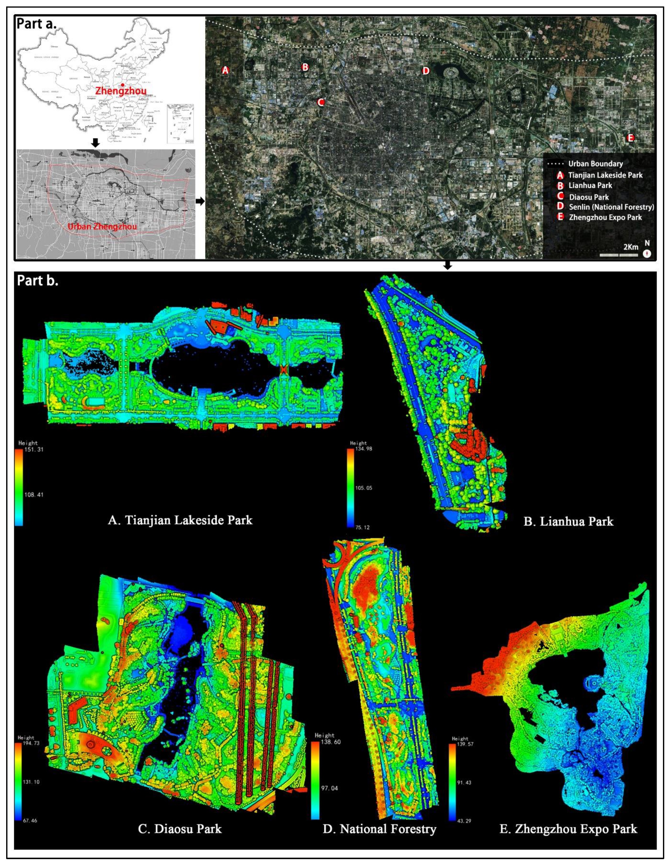
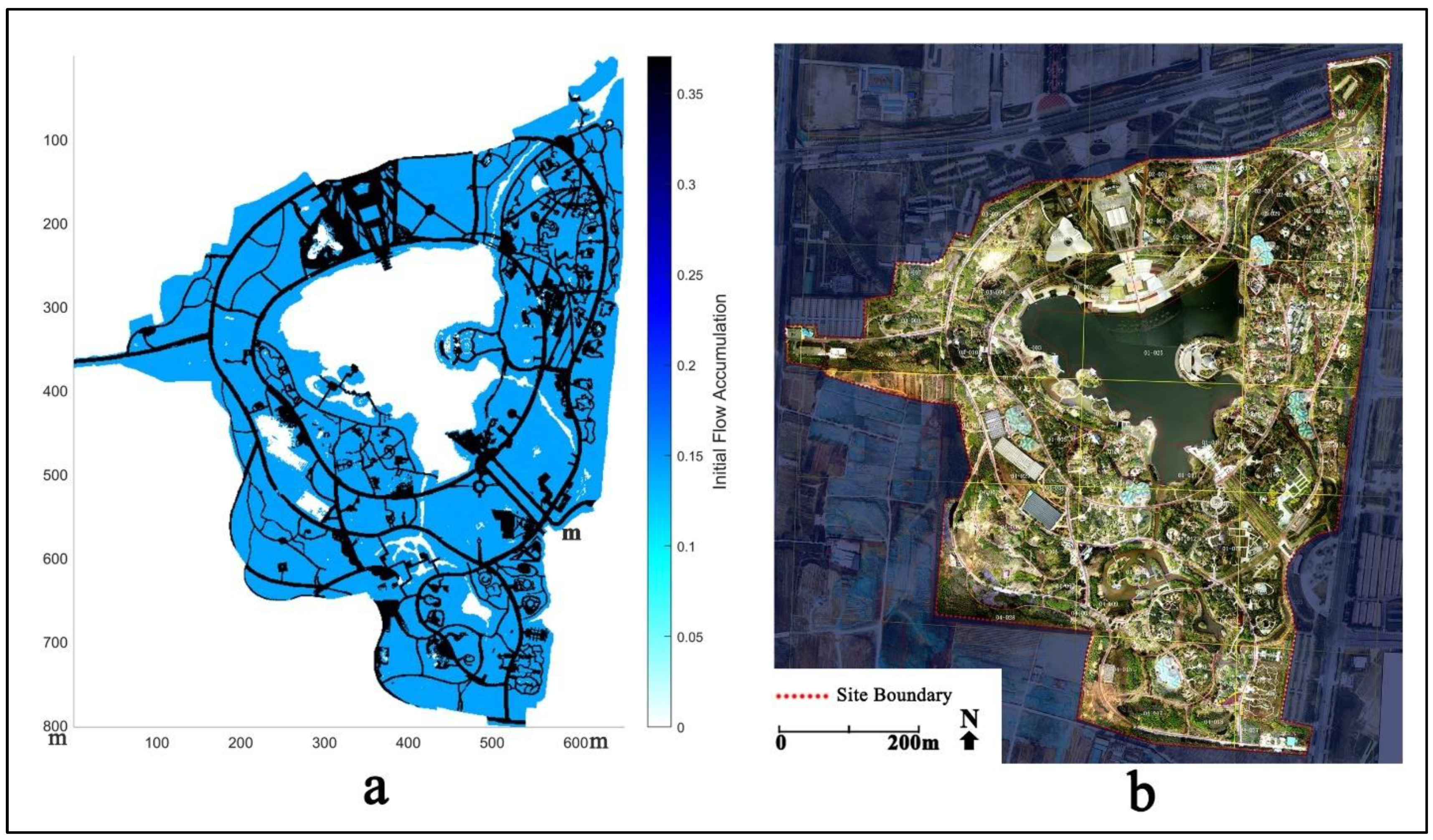
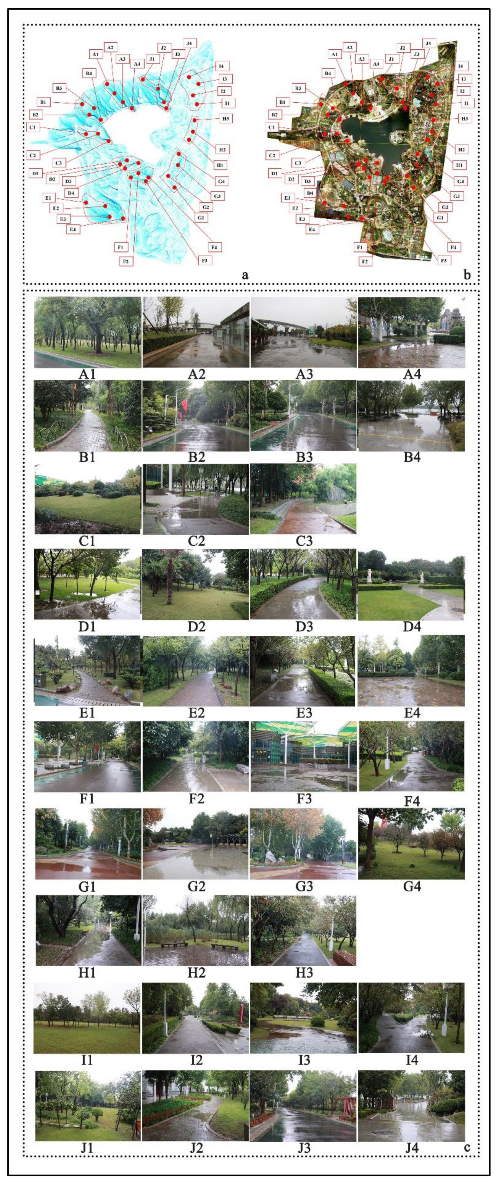
2.1. Study Sites

The study site considered in this work is in Easton Zhengzhou, Henan Province; this area has a warm, temperate, continental monsoon climate. The annual average temperature in the study area is 14.5 °C, with a precipitation amount of 60 mm and sandy loam soils in the urban region [23]. The LiDAR scanning region and modeling area of the study site include 5 urban green spaces with a total area of 830 hm2. The drainage of these sites relies on soil infiltration and surface artesian flow. The general water catchment direction is towards the central lake or ponds, and hard pavement areas are not contained within the city drainage network. The drainage method at the study sites represents that of typical urban green spaces in Zhengzhou. Figure 1 shows the locations and LiDAR images of the study sites.

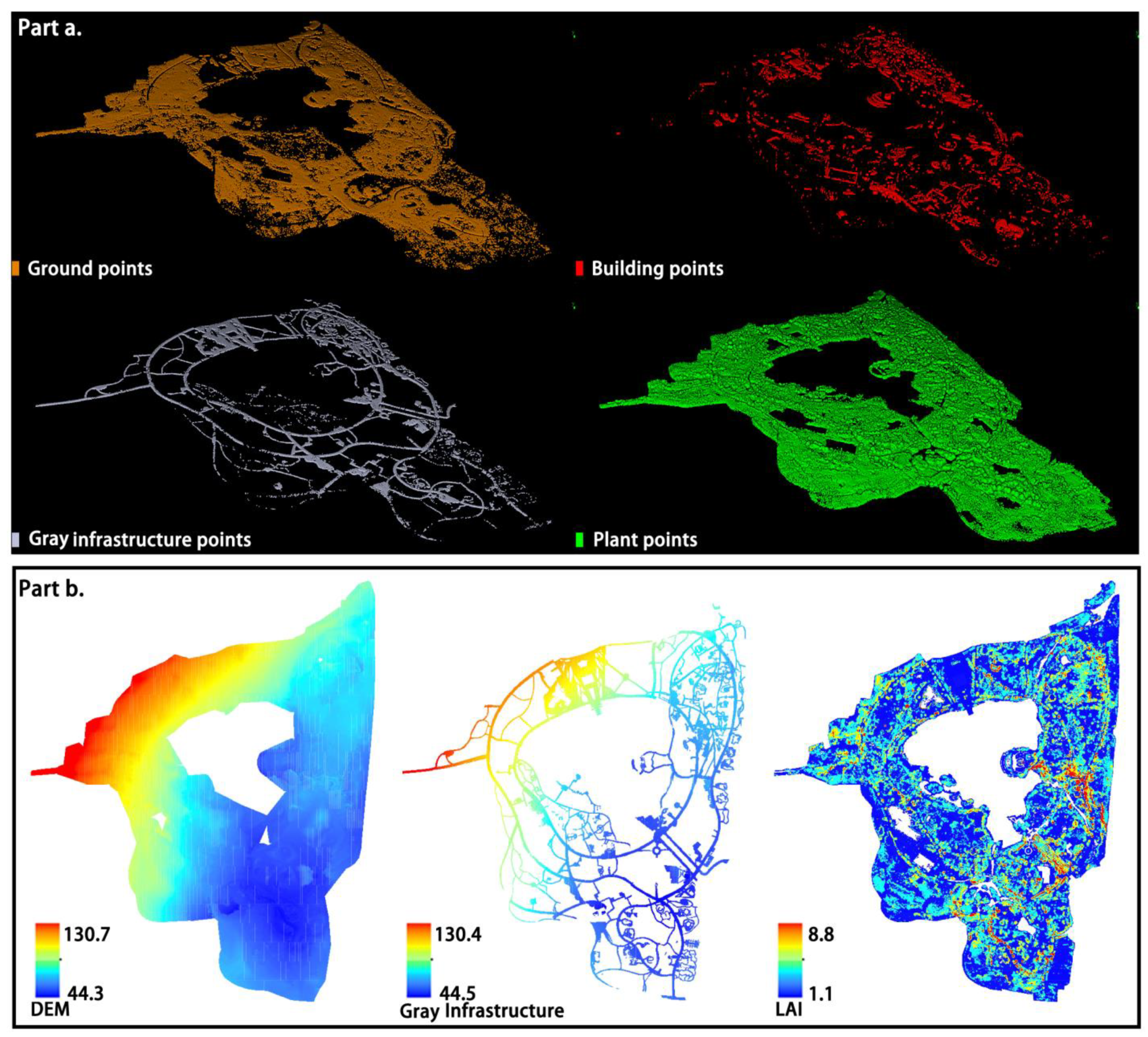
2.2. LiDAR Data Preparation for Use in MATLAB

Point cloud data were obtained from a combination of backpack and airborne LiDAR devices from Beijing Green Valley Technology Co., Ltd. (Beijing, China). The point cloud data were processed in LiDAR 360 V4.1 software. The LiDAR data representing the study sites were collected from June–August 2021 during the leaf-on period. The standard point cloud data specifications included denoising and normalization, and LiDAR 360 data specifications, were applied to the data characterization of each site.
The point clouds of each site were classified into 4 types based on their characteristics: ground surfaces, buildings, gray infrastructure, and plants (Figure 2a). The ground points were used to generate the DEM and provide the basic surface information for the subsequent surface runoff modeling. The gray infrastructure points included the roads and squares in each site and formed an attribute subdivision of the ground points; this subdivision was then used to distinguish the hard and soft surfaces (e.g., soil). Gray infrastructure encompasses impermeable surfaces, and the rainwater that falls on such areas does not experience surface infiltration; in contrast, over soft surfaces, the infiltration of rainwater should be considered. The building points were used mainly to separate the remaining ground features, except vegetation, among the surface points and to mark the building positions in the DEM group to facilitate the reconstruction of the building boundaries. The plant points were used to derive the canopy leaf area index (LAI), which subsequently calculates canopy interception and evaporation.
Using LiDAR360 V4.0 software, a digital information model composed of DEM and DSM datasets was constructed (Figure 2b). According to the characteristics of the overall flat terrain but rich microtopography of the analyzed parks, the iso-height distance of the elevation layers in the DEM dataset was set to 1 m with a resolution of 2 m × 2 m grid cells [24]. This resolution was the highest that could be supported by computer memory at this stage of research at the park scale. The DSM dataset was generated based on the gray infrastructure and vegetation point clouds; in this dataset, “pixelated” (2 m × 2 m) gray infrastructure and LAI data layers were constructed within each grid cell, and these layers were matched with the DEM grids. Therefore, each grid cell contained 3 parameter layers: elevation, gray infrastructure, and LAI. When the LAI was equal to 0, the cell was defined as a ground cover plant grid cell, and the rainwater interception effect of the vegetation canopy was not considered. When gray infrastructure filled a grid cell, the surface infiltration effect was not considered in that cell.

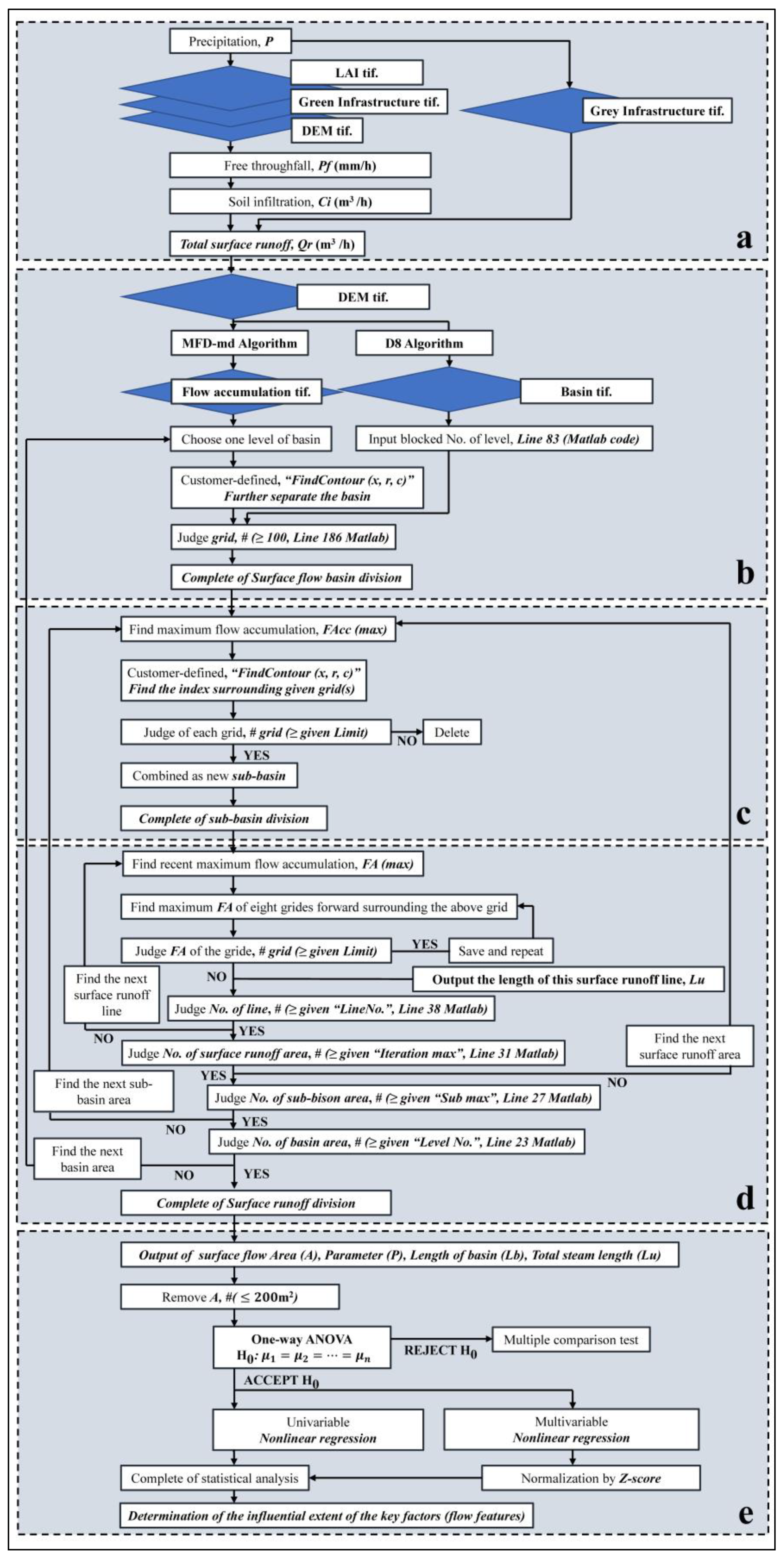
2.3. Technical Route

To build the fitting relationship between the morphological factors of a flow basin and its quantified FA, this research had six objectives (Figure 3): Steps (b) to (d) are together called the “extraction algorithm”.

2.4. Precipitation to Surface Runoff Simulation

To accumulate the surface runoff in urban green spaces precisely at the 2 m × 2 m grid scale, the UFORE-Hydro model was applied to consider the interception and infiltration effects of the tree canopy and soft surface (soil), respectively. The evaporation amounts induced by the canopy and soil surface were also simulated to measure their absorption accommodation capacities during precipitation events. The surface runoff calculation included two steps: (a) canopy interception and evaporation and (b) soil infiltration and evaporation.

2.4.1. Canopy Interception

The interception of precipitation by the canopy is controlled by both weather dynamics (precipitation intensity and duration) and tree characteristics (leaf area, storage capacity, and initial storage). The canopy interception equation is expressed as follows:
Δ C Δ t = P P f E
where C (mm) is the depth of water on the unit canopy at time t, P (mm/h) is the precipitation, Pf (mm/h) represents the below-canopy free-throughfall precipitation reaching the ground, and E (mm/h) is the evaporation rate from the wet canopy. The storage capacity, S, is equal to the maximum value of C, Cmax, of the forest canopy, as linearly related to the LAI [6]; this term can be expressed as follows:
S = {                                               S L L A I , ( M a y O c t . ) S L L A I α ( S L L A I ) , ( N o v . A p r . )
where SL (mm) represents the specific leaf storage coefficient, which in the UFORE-Hydro model defaults to an average value of 0.2 mm. In this article, we referenced the point-cloud LAI simulated in every 2 m × 2 m grid cell to calculate the S capacity in each site plot. In the above equations, α represents the LAI adjustment coefficient in the winter season (leaf-off period). For deciduous trees, the LAI is a dynamic index and is the smallest in winter. We referenced the canopy interception ratio function between summer and winter to calculate the value of α as follows:
α = 0.00008 P 2 0.0123 P + 0.781

2.4.2. Canopy Evaporation

As the water intercepted by the canopy evaporates, the canopy water storage capacity is restored and updated. The evaporation flux, Ec (mm), is simulated as follows [25,26]:
E c = { ( C S ) 2 3 E p ,         C < S                           E p ,         C S
where Ep is the potential evaporation coefficient of the canopy, which is set here to 0.2 mm/h; this term is described as the average evaporation potential of trees and shrubs and is derived from the modified Penman–Monteith equation [27]. The Ec equation applied in this research is defined as follows: when P is greater than S, the overloaded precipitation (CS) is recognized as free throughfall reaching the ground and does not participate in canopy evaporation.

2.4.3. Free Throughfall

In the canopy fraction of the watershed and at the first stage of interception, which spans from the start of precipitation until the canopy storage capacity (S) and Cmax are reached, the forest canopy intercepts most of the falling precipitation. The UFORE-Hydro model allows no rainwater to pass through the canopy before S reaches its maximum. The second stage starts when the stored rainfall is equal to S with no further interception and all subsequent precipitation reaches the ground as free throughfall Pf, which is calculated as follows:
P f = {                                             0 , P < ( S + E c ) P ( S + E c ) , P ( S + E c )

2.4.4. Steady Infiltration Rate

The UFORE-Hydro model uses the Green-Ampt infiltration theory together with the infiltration concept and excess saturation processes of TOPMODEL [28,29]. Considering the sandy loam soils found in the Yellow River basin area of Zhengzhou, we referenced the sand-layered improved Green-Ampt equation to describe the steady soil infiltration rate (Ir) as follows:
I r = C w K s ( h + S m Z + 1 )
where C w represents the hydraulic conductivity coefficient, which ranges from 0.91 to 0.99 in most research. In this article, we set this term to 0.95 based on sandy soil experiments [7]. K s , the saturated hydraulic conductivity of the upper-layer soil, was set to 0.01 mm/s [30]. The terms h and S m represent the pressure head (30 mm) and the average water entry suction (3.12), respectively [31,32]. Z is the depth of the sandy layer; this term was set to 250 mm here based on the site surveys. The soil infiltration amount ( C i ) in the study period ( Δ t ) is expressed as Δ t I r (mm), and any amount of water ( P f ) over C i results in overinfiltration of surface runoff ( Q o ):
Q o = {                           0 ,     P f   < Δ t I r P f Δ t I r ,   P f   Δ t I r

2.4.5. Soil Storage Capacity

Soil water storage is a dynamic value that depends on the difference between the soil saturated moisture capacity ( S s ) and the field moisture capacity ( ω ). Considering the soil cover depth of 75–120 cm in the research area, we selected 100 cm as the average depth to calculate the soil storage capacity S i :
S i = ( S s ω ) P b S v
where S s is 336.25 g/kg, ω is 305.05 g/kg, and P b represents the soil bulk density, which was set here to 1.42 g/cm3. The soil values listed above were selected in reference to farmland soil investigations performed in the Zhengzhou region [8].

2.4.6. Soil Evaporation

Considering that most of the soil surfaces of the green space at the research site were covered with grasses, as the ground cover type, we adopted the preferred method for estimating the potential evaporation rate, E rc , from the referenced crop of short, actively growing grass:
E r c = F r c 1 A + F r c 2 D ¯
where F rc 1 and F rc 2 are the function coefficients of the temperature and wind speed at the study site, which were set here to 0.293 and 4.495, respectively, based on the geographic features of the research site at elevations of 0–100 m and annual temperatures of 10–15 °C [27]. A is the energy available for evaporation, which was set to 15.0; this value corresponds to a latitude of 30° N, which is close to the latitudes of the research sites ranging from 34°44′ to 34°45′ N. D ¯ is the average vapor pressure (kPa). The evaporation value at the study sites can be described as follows:
E i = { ( C i S i ) E r c ,   C i < S i                     E r c , C i S i

2.4.7. Surface Runoff

When the soil infiltration amount ( C i ) is greater than S i , overstorage is reached, and surface runoff ( Q s ) occurs; this relationship can be expressed as follows:
Q s = {                                                         0 , Δ t I r < ( S i + E i ) Δ t I r ( S i + E i ) , Δ t I r ( S i + E i )
The total soft surface (soil) area surface runoff amount, Q r , is calculated as the sum of the overinfiltration ( Q s )   and overstorage runoff ( Q o ) amounts:
Q r = Q s + Q o

2.5. Surface Flow and Water Accumulation Simulations

The parameterized mesh division of the study sites, forming 2 m × 2 m grids, allowed the unique surface runoff value in each grid to be generated during each precipitation event and provided the precision runoff amount after the interception, infiltration, and evaporation steps at the park scale, thus facilitating the simulation of the runoff water path and storage district in different rainfall intensities. This part included two sections: (a) the flow partition exponential function and (b) the digital grid surface diversion function.

2.5.1. Exponential Flow Partitioning Function

The maximum downslope gradient was used to determine the function f ( e )   of the flow partition index to simulate the effect of the maximum downslope gradient on the flow partition:
f ( e ) = {                                                                                 p l ;   ( e e m i n ) e e m i n e m a x e m i n × ( p u p l ) + p l ;   ( e m i n < e < e m a x )                                                                                 p u ;   ( e e m a x )
where e is the tangent of the maximum downslope gradient; f ( e ) is the flow partition function; p u and p l are the upper and lower limits of f ( e ) and are used as p values representing fully divergent and convergent flows, respectively; and e min and e max are the e-values associated with p l and p u , respectively. The boundaries of f ( e ) (i.e., p u   and p l ) are defined in the domain of [1.1, 10], depending on the best-value comparison of the flow-partitioning index identified by most scholars to simulate the complete divergence or convergence of the flow. The above equation can be simplified by adjusting some settings to modify the flow partition function in the general MFD algorithm, as follows [14]:
f ( e ) = 8.9 × m i n ( e , 1 ) + 1.1

2.5.2. Digital Grid Surface Diversion Function

MFD-md is a multiflow runoff distribution algorithm, the core purpose of which is to describe the closest possible surface runoff distribution to the real situation around a high-level surface grid DEM. This algorithm can be expressed as follows:
d i = { ( t a n   β i ) f ( e ) × L i j = 1 8 ( t a n   β j ) f ( e ) × L j
where d i is the proportion flowing into the i-th adjacent cell; tan   β i is the slope gradient of the i-th adjacent cell; L i is the “effective contour length” of digital grid i; and f ( e ) is calculated by Equation (14).

2.6. Morphometric Parameter Quantification and Feature Clustering of the Flow Basin

The built-in D8 runoff algorithm of ArcGIS V10.8 was used herein to guide the generated basin division function and perform the basin identification and boundary division steps for the analyzed urban spaces at different scales. First, we imported the basin-delineated.tiff file representing the study area into MATLAB; then, we superimposed the surface FA data layer applied to the MFD-md result in each basin (Figure 4). Thus, we extracted the characteristic parameters of the basin based on the surface runoff accumulation parameters.
To extract each flow basin (Figure 3b), the user-defined function “Find Contour” was used to find the coordinate index of the contour value surrounding the given inner points with the additional consideration of the study area boundaries; that is, the outside coordinates were not given until all grid cells surrounding the target point and satisfying the D8 index value were found. Similarly, users can determine the minimum number of neglectable grid cells in the target flow basin in Line 186 of the MATLAB code; that is, a relatively small area can be neglected. The flow basin structure includes the following basic features:

2.6.1. Flow Area

The size of the flow area (A) was calculated by multiplying the number of grid cells in the extracted flow basins by the area of one grid cell (i.e., 2 m × 2 m). Notably, the determination of the neglectable target flow basin defined by users in Line 186 of the MATLAB code is the minimum number of neglectable grid cells rather than a portion of the target area.

2.6.2. Flow Perimeter
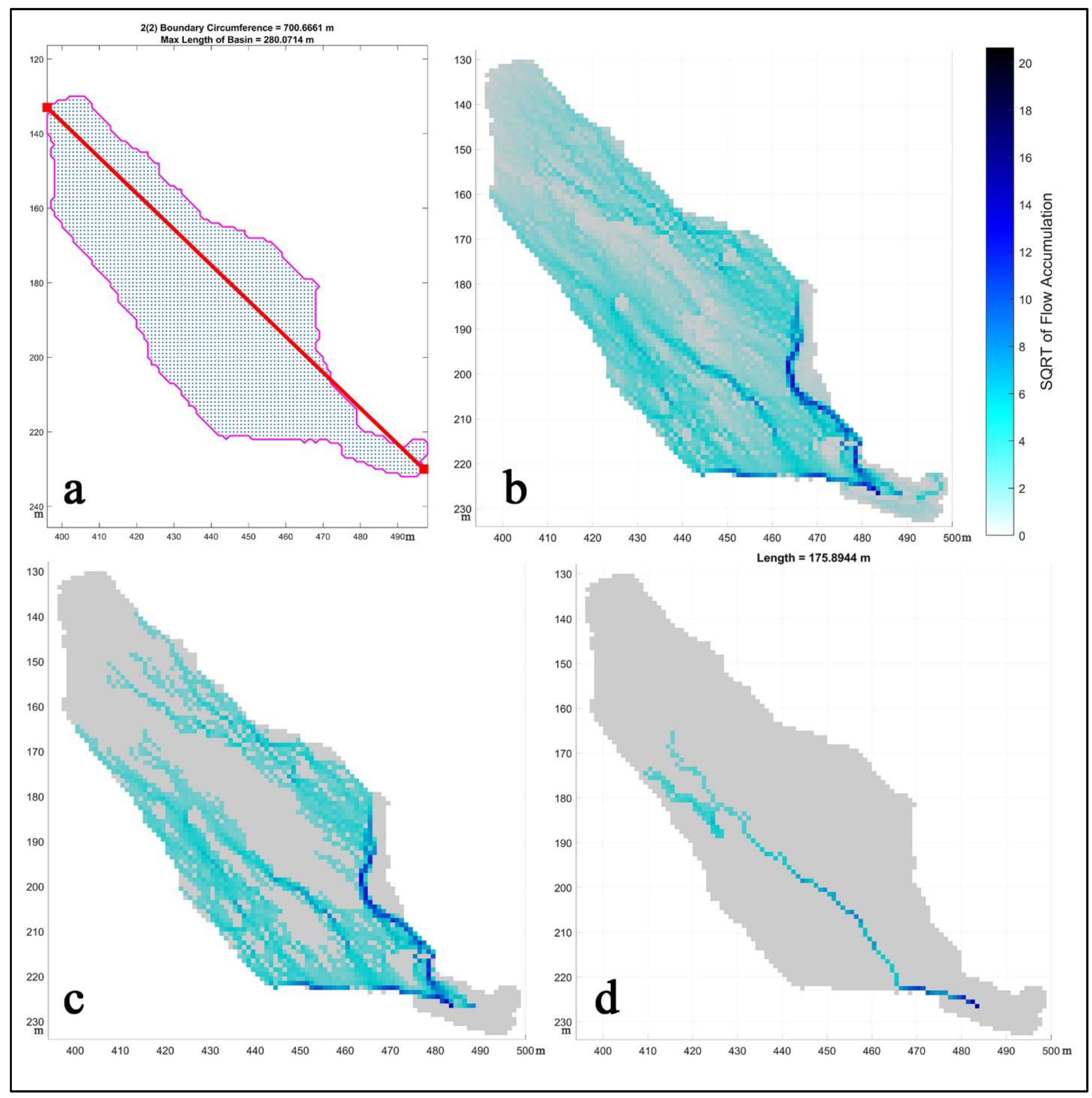
The process used to calculate the flow perimeter (P) consisted of two steps: (1) the built-in “boundary” function in MATLAB was used to find the boundary coordinates of the extracted flow basins; (2) the built-in “perimeter” function in MATLAB was utilized to calculate the summation of two adjacent points surrounding the flow basin, i.e., the circumference of the target flow basin.

2.6.3. Basin Length

Based on the use of the built-in “boundary” function in MATLAB to find the boundary coordinates of the extracted flow basin, we found the maximum Euclidean distance by calculating the boundaries between every coordinate pair; moreover, we obtained the corresponding coordinates of the two locations. The perimeter and basin-length ( L b ) results are shown in one plot (Figure 5a).

2.6.4. Stream Length

The maximum FA among the eight grid cells surrounding the maximum-flow-accumulation cell (set as the initial point) in the extracted flow basin was chosen as the second point; then, the maximum FA among the five grids surrounding the previous point was chosen as the next target point to prevent acute-angle flows from arising during the stream-extraction process (Figure 5d). In this way, we obtained the stream length ( L u ) by summing the Euclidean distances between each pair of adjacent points after successfully extracting a suitable stream in each extracted flow basin. Similarly, users can determine the minimum value of the neglectable stream length in Line 313 of the MATLAB code.

2.7. Obtaining Univariable Nonlinear Regression Models and Some Suitable Multivariable Nonlinear Regression Models with the Goodness-of-Fit Information Criterion

One-way analysis of variance (one-way ANOVA) was used to test the difference between two or more means of given green spaces whose null hypothesis is that the mean FA of each individual green space is significantly equal to those of other green spaces, i.e., H 0 :   μ 1 = μ 2 = = μ n . Accepting this null hypothesis simplifies the modeling and simulation processes. Once the null hypothesis is rejected at a given significance level, users can alternatively examine the concrete discrepancies between two green spaces by clicking on one of the green-space names in the plot of multiple comparisons of means (Figure 6).
Six sigmoid nonlinear regression curves are typically applied in statistical research as alternative functions (listed in Table 1) fitted to the univariable series to represent all available area, perimeter, maximum basin length, and total basin-scale stream length data, but only some of these curves effectively fitted the multivariable nonlinear regression series of the linear combination of the above variables, possibly due to algorithm restrictions and data scarcity, despite our attempts to use diverse algorithms and select optimal initial values for each estimated coefficient. For every regression model and robust weight function, the estimated coefficient value and standard error were saved in a corresponding Excel file. In addition, the t-statistic was obtained with the null hypothesis that the coefficient is zero to further choose and/or reject suitable independent variables. Moreover, the p values of the corresponding t-statistics were obtained. Additionally, several robust weight functions (Table 2) were utilized to fit the multivariable nonlinear regression model, and the value of the goodness-of-fit information criterion (see Table 3 for details) is also listed in Supplementary Material Tables S1 and S2.

3. Results

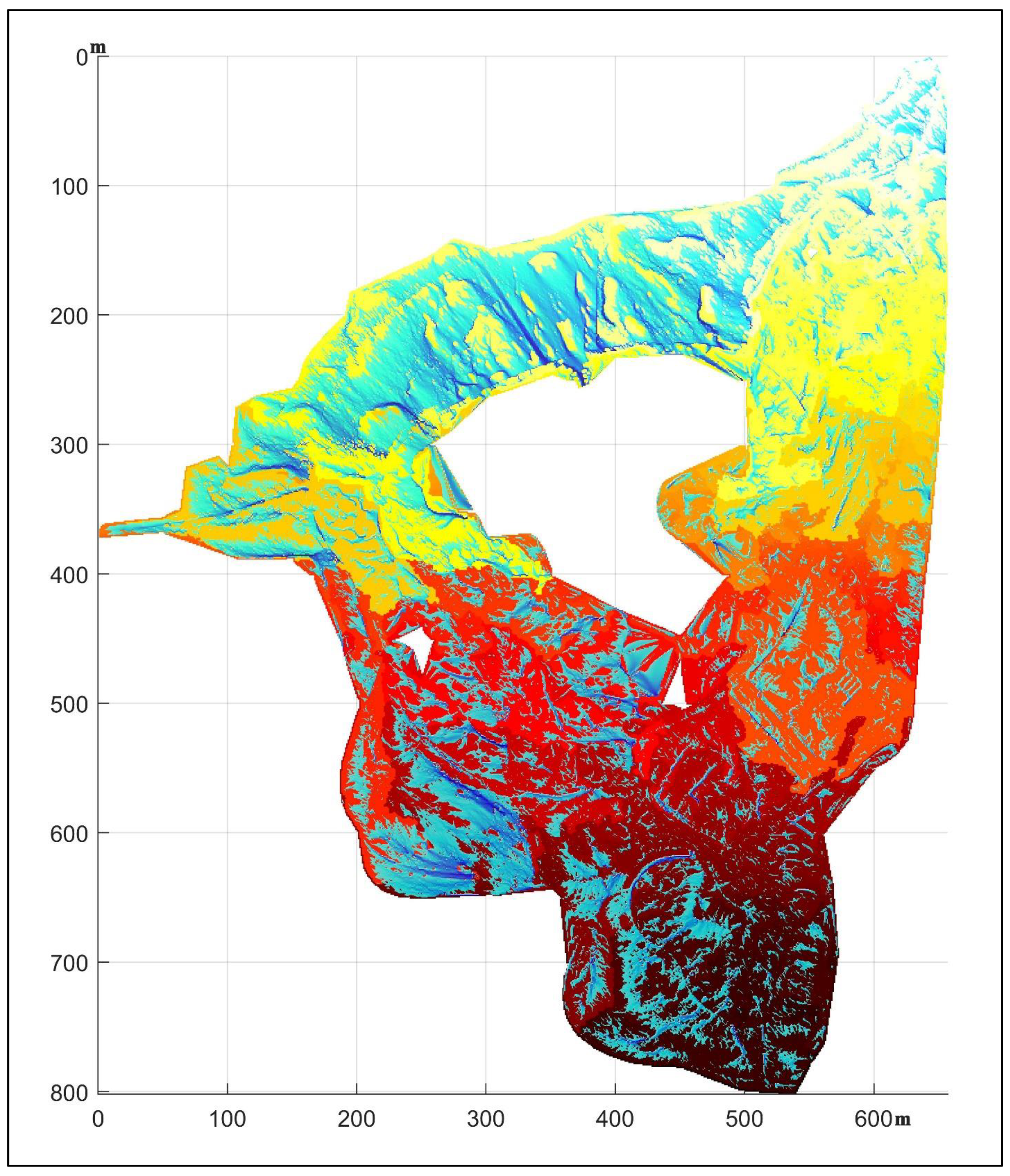
3.1. Verification of the FA Results of the UFORE-Hydro and Coupled MFD-md Algorithms in the Analyzed Urban Green Spaces

The typical daily average rainstorm precipitation (100 mm/24 h) recorded by the Zhengzhou Meteorological Bureau from 2015 to 2019, according to the National Meteorological Administration’s Rainfall Intensity Grade Standard (GB/T 28592-2012), was used as the precipitation input data in this work [33]. After the canopy interception and soil infiltration simulation via UFORE-Hydro, the surface runoff value in each grid cell showed a unique parameter that could potentially facilitate a more precise surface flow route and water catchment simulations. Compared with the site orthophoto image, in the grid cells containing impervious areas, including park roads and squares, the amount of surface runoff (greater than 0.3 m3) was generally higher than that in soft-soil areas (less than 0.2 m3), indicating fair agreement with the real surface runoff situation at the park scale (Figure 7).
The consistency between the theoretical results by applying the UFORE-Hydro model and MFD-md algorithms in MATLAB and the realistic rainfall surface water catchment situation in Zhengzhou Expo Park was demonstrated (Figure 8). There were 10 surface flow sections (from A–J) over the park, and a total of 38 test plots were applied for verification. After experiencing continuous rainfall at a rate of 2.0 mm/h for 4 h in October 2022, 3 types of flow runoff appeared in the park: initial flow, inflow, and water catchment. In Figure 8c, images A1, B1, C1, D2, D4, E1, E2, F1, F2, G4, H3, I1, I2, and J1 show the initial flow type; images A2, A3, B2, B3, C2, G2, G3, H2, I4, and J2 depict the inflow type; and images A4, B4, C3, D1, D3, E3, E4, F3, F4, G1, H1, I3, J3, and J4 show the water catchment type at the test site. We found that the theoretical simulation results could match the real situation of flowing water at the study site following rainfall. In Figure 8a, the flow route in light blue shows the initial flow, and the area in dark blue shows the surface water catchment.

3.2. Morphometric Parameter Quantification and Feature Results of the Surface Flow Basin in the Analyzed Urban Green Spaces

The morphometric parameters were automatically computed and stored in an Excel file named “Final Results Sum”. This file included the maximum basin length ( L b ) and the sum of the stream length ( L u ), which are visualized in Figure 5a–d. The L u parameter was calculated by aggregating the lengths of each stream in the flow basin. The calculated values of L u were systematically organized in the Excel file, with each row containing a complete set of parameters following the three aforementioned ones ( A , P , and L b ). Figure 5b–d displays not only the approximate contours of the flow basins but also the relative locations of the two ends of the maximum Euclidean distance. Consequently, users can utilize the range of (x, y)-axis coordinates to identify the relative location of each flow basin.
As a result of the clustering analysis, the theoretical data yielded from the five classical urban green spaces were separated into two groups: “small basins” and “large basins”. It was roughly concluded that the critical value for separating these two green space categories was approximately 9000 m2; that is, areas smaller than this value were “small basins”, while green spaces larger than this value were considered “large basins”. In addition, the maximum basin length, one of the morphometric parameters that was considered, could be used to explicitly divide the basins into two different kinds. However, the two other morphometric parameters (the basin circumference and the sum of the stream length) likely cannot be used as a sole reference standard, as some of the results obtained from these parameters were consistent with the middle-range area and were thus regarded as “large basins”, while their stream lengths were in the interval of “small basins” (i.e., L u   < 1100 m). Similar results were obtained using the basin circumference.

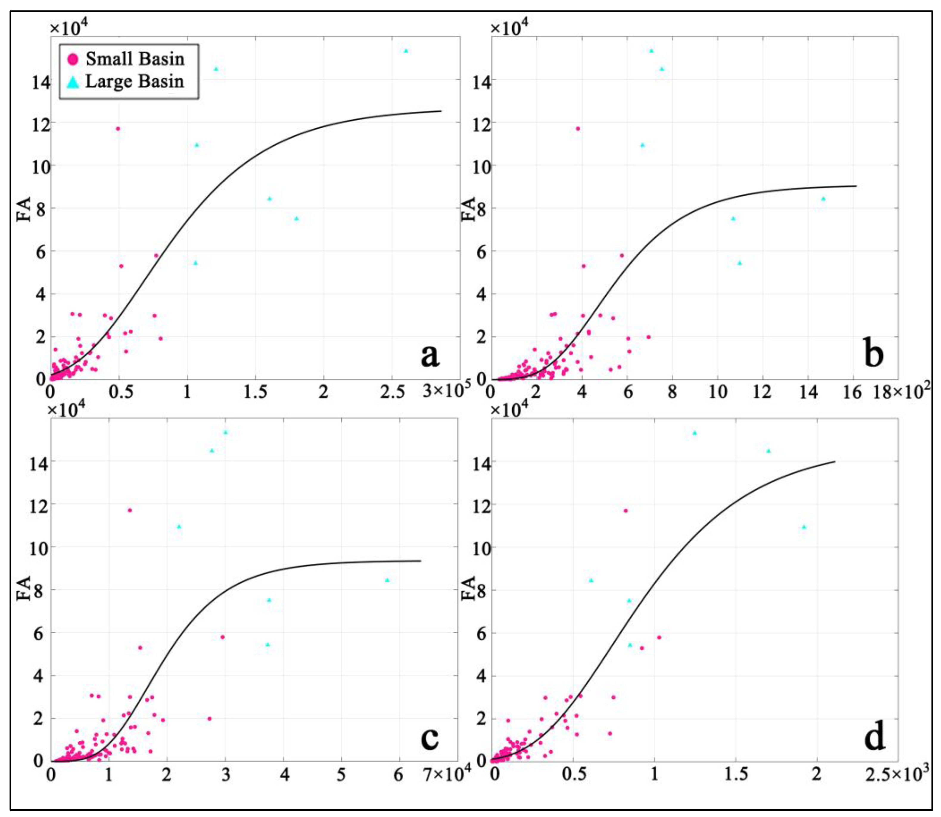
3.3. Determination of the Model Results and the Statistical Interpretation

One-way ANOVA was used to assess the differences among the five given green spaces, indicating that no significant difference existed among the analyzed green spaces, i.e., all the analyzed green spaces could be regarded as a single urban green space category, thus simplifying the modeling and simulation processes without considering the discrepancies among the analyzed green spaces. In the univariable analysis results, the vast majority of the six nonlinear regression models without any weight function fitted to the four independent variables (the basin area, circumference, maximum basin length, and sum of the stream lengths) depicted the sigmoid variation trend (Figure 9). Three nonlinear functions yielded converging results: the logistic, modified logistic, and Gompertz functions.
By comparing the previously mentioned information criteria (such as the AIC, AICc, and R2) between different models under the same weight function based on the multivariable nonlinear regression results and while considering the significant features of each estimated coefficient, we eventually determined the following model statistics to predict the FA characteristics with the variations in the basin area, circumference, maximum basin length, and sum of the stream lengths among the studied green spaces. The Gompertz function was applied, and the “fair” weight function, which is expressed as follows, was added:
F A = 1.810 × 10 5 e 4.603 e ( 7.361 × 10 6 A + 1.0784 × 10 4 P 4.413 × 10 4 L b + 9.906 × 10 4 L u )
where variables A (in m2), P (in m), L b (in m), and L u (in m) are the independent variables listed above, and F A (a relative number) represents the flow accumulation of one of the studied basins. Adding the “fair” weight function to the Gompertz function provided a relatively high R2 value (0.9565) compared to that of most of the other functions, indicating that approximately 95.65% of the total dependent variable results (FA) could be explained by the four independent variables (the basin area, circumference, maximum basin length, and sum of the stream length).
For the detection of the actual influential extent of each morphometric parameter on surface FA, we applied the normalized z score to fit the nonlinear regression model with the same weight function as that applied to the above theoretical data. This model can be expressed as follows:
F A ˜ = 5.739 e 5.4506 e ( 0.4208 A ˜ + 0.1727 P ˜ 0.2729 L b ˜ + 0.4689 L u ˜ )
where the tilde on each variable represents the normalized z score.
The normalized-function results indicated that the morphometric parameters of the basin area and the sum of the interior stream lengths had almost equally important effects on the FA results; the extent of the influence of each of these parameters was approximately 2.5 times that of the basin circumference.

4. Discussion

4.1. Analysis of the Impact of Basin Features on Surface Runoff Accumulation

Our research findings demonstrate a general nonlinear (Gompertz) regression relationship between flow accumulation (FA) and basin morphometric parameters. Specifically, within a certain range, an increase in the size of the morphometric features can significantly enhance the FA of the basin. Various studies focusing on the quantification and evaluation of basin morphometric parameters have highlighted that an increase in the stream order class can substantially improve the water storage capacity of the catchment area [28,29,30]. Furthermore, expanding significant basin features such as Area (A) and Perimeter (P) directly contributes to the increase in stream numbers, thus promoting a rise in stream orders [31]. Therefore, considering the common occurrence of small and fragmented basins in park green spaces, adjustments in elevation that connect and expand these smaller basins into a larger one could effectively enhance water storage capacity.
One similar study found that the declines in urban flooding probabilities observed in some districts with wide green space areas indicated that increasing the green-space area is an effective approach to decrease the flooding probability to varying extents [32]. However, according to the features of the sigmoid curves between the FA and basin features, interminably expanding the areas of green spaces does not seem to be a practical means of reducing flood risks because of limitations of the total urban green proportion of approximately 35% in most Chinese cities [34]. Therefore, it has already been demonstrated that not only area occupation but also increasing stream density and connections positively promote runoff regulation and water division potentials, with some limitations, to achieve the goal of improving the water storage capacity in green spaces [6]. The result of increasing stream density highlighted the increase in total stream length, which in turn increased the water capacity in a fixed area basin. Additionally, the maximum basin length showed a negative effect on the FA results under identical basin circumferences. One possible reason is that a redundant basin length results in a relatively narrow basin shape that does not contribute to the formation of branch surface runoff and is not conducive to the formation of water ponds.

4.2. Recommended Strategies for Reducing Urban Flooding Risks

Many efficient guiding principles have been suggested, and it is generally accepted that regulating topographic design can increase the rainwater storage capacity in urban green space and efficiently reduce flood potential under extremely severe weather conditions in urban greening areas [35,36,37]. The combined surface FA and basin feature equation (Equation (16)) can be used to quantify the static capacities of water storage in green spaces. Additionally, this approach promotes the understanding of how to accurately design the topographic features and sizes of green infrastructures to achieve water storage capacity improvements. Our research suggests that combining small watersheds into a large basin efficiently increases the water storage capacity. Related research on basin parameters shows that increasing the basin area from 1100 m2 to 1720 m2 can yield an 86% improvement in the water storage capacity (from 1130 m3 to 2100 m3) [38]. Quantitative data show that watersheds less than 2 hm2 should be combined with nearby basins to increase the overall basin size and efficiently promote the water storage capacity. The total stream length in an area of fixed green space, which is influenced by the density of surface flows, is also a key feature related to water storage. Decreasing the stream density by 4.6% can lead to a 35% decrease in the water storage capacity in the river ecosystem [39]. Our results indicate that a total stream length greater than 300 m will dramatically increase the water storage ability of the inner basin.
In addition, from the perspective of integrated urban areas rather than a park scale, other researchers who have built relevant models have stated that the alleviation effect of a single green infrastructure would reduce the flooding risk, especially under storm rainfall conditions [40]. Therefore, a long-term green infrastructure system plan should be emphasized in the urbanization process, and a major focus should be placed on the network construction of urban green spaces to reduce the risks of urban waterlogging and flood disasters [41]. Furthermore, the DSM also performs efficiently in increasing the water storage capacity, and the areas of plants with relatively high LAIs should be suitably increased, as this could increase the canopy interception of light rainfall and delay the generation time of surface flood peaks during storm events. Impermeable surfaces could be replaced with porous brick or other permeable surfaces (soil) to increase infiltration and reduce the generation of surface runoff [40,42].

5. Conclusions

The UFORE-Hydro and MFD-md hydrology algorithms utilized to allocate precipitation to runoff based on the LAI, ground material (soil or GI), and elevation of the grid cells precisely expressed the tiny discrepancy in the net surface runoff in the different categories of ground cover. The simulation results exhibited fair agreement with the actual scenario (Figure 9). The one-way ANOVA tests performed to assess the differences among the five given green spaces indicated that the mean FA obtained from the individual green spaces was significantly equal (p value > 0.05, Figure 6). Following the technical extraction route of surface flow basin morphologies built up via MATLAB code, several flow basins from the five green spaces were clustered into two categories using the k-means algorithm under unsupervised learning. Six common nonlinear regression functions were applied in the univariable analysis, most of which showed relatively high explanatory abilities for FA variations.
Moreover, three nonlinear regression functions were fitted to the theoretical data of four fundamental morphometric parameters in the multivariable analysis. The Gompertz function (Equation (16)) with the “fair” weight function was eventually selected to compare the information criteria, which had a 95.65% explanation capacity, i.e., the dependent variable (FA) could be explained by the four independent variables (the basin area, circumference, maximum basin length, and total stream lengths). Furthermore, z score normalization was applied using the same function as that listed above along with the weight function to obtain Equation (17), resulting in the total stream length in the basin and the basin area being two almost equally essential factors in determining the water-storage ability of the analyzed basins, followed by the basin circumference. In contrast, the maximum length of the basin showed a negative correlation.
We developed univariable and multivariable regression models to fit the FA and four basin morphometric parameters individually or simultaneously. The results theoretically provide urban designers with quantitative topographic and vertical design guidelines aimed at improving the water storage capacity, not only for individual basins but also for integrated green spaces. As a limitation of this study, our developed model considered only independent park-scale green space but neglected the synthetic function of landscape connectivity. Therefore, future research should be determined through comprehensive consideration involving the basin morphological features in different land use types (such as roads, residential, and commercial areas) and regions of block and urban scales to explore theoretical optimization algorithms and the scientific allocation of land resources.

Supplementary Materials

The following supporting information can be downloaded at: https://www.mdpi.com/article/10.3390/w15132442/s1, Figure S1: Main MATLAB Code, developed in MATLAB, R2021a (9.10.0.16028826); Table S1: Univariable nonlinear regression coefficients estimated without the weight function and the corresponding information criterion; Table S2: Multivariable nonlinear regression coefficients estimated with different weight functions and the corresponding information criterion.

Author Contributions

Conceptualization, G.T., H.H. and Y.L.; methodology, H.H.; software, H.H., Y.T. and Y.L.; validation, H.H., Y.L. and G.T.; formal analysis, A.C.A. and S.G.C.; investigation, M.W.; resources, P.W.; data curation, M.W. and X.J.; writing—original draft preparation, H.H. and Y.L.; writing—review and editing, A.C.A., H.H. and S.G.C.; visualization, H.H. and Y.L.; supervision, G.T.; project administration, G.T.; funding acquisition, Y.L. All authors have read and agreed to the published version of the manuscript.

Funding

This research was funded by the Ministry of Education of the People’s Republic of China [grant number HZKY20220274], the Henan Province Science and Technology Research Project [grant number 222102520031], the Henan Province Science and Technology Research Project [grant number 232102320187], the Key Projects of the Henan Provincial Department of Education [grant number 21A220002], and the Henan Province University Discipline Innovation Base [grant numbers CXJD2021004 and GXJD006].

Institutional Review Board Statement

Not applicable.

Informed Consent Statement

Not applicable.

Data Availability Statement

The park LiDAR data were collected and supported by the Henan Provincial Joint International Research Laboratory of Landscape Architecture in the College of Landscape Architecture and Art, Henan Agricultural University. The daily average precipitation data were recorded by the Zhengzhou Meteorological Bureau and are available at http://ha.cma.gov.cn/ (accessed on 16 November 2022).

Acknowledgments

This research is supported by the Henan Provincial Joint International Research Laboratory of Landscape Architecture and the Zhengzhou Green Expo Park Management Center.

Conflicts of Interest

The authors declare no conflict of interest.

References

  1. Dong, X.; Guo, H.; Zeng, S. Enhancing future resilience in urban drainage system: Green versus grey infrastructure. Water Res. 2017, 124, 280–289. [Google Scholar] [CrossRef] [PubMed]
  2. Alves, A.; Gersonius, B.; Kapelan, Z.; Vojinovic, Z.; Sanchez, A. Assessing the co-benefits of green-blue-grey infrastructure for sustainable urban flood risk management. J. Environ. Manag. 2019, 239, 244–254. [Google Scholar] [CrossRef] [PubMed]
  3. Xu, Z.; Xiong, L.; Li, H.; Xu, J.; Cai, X.; Chen, K.; Wu, J. Runoff simulation of two typical urban green land types with the Stormwater Management Model (SWMM): Sensitivity analysis and calibration of runoff parameters. Environ. Monit. Assess. 2019, 191, 343. [Google Scholar] [CrossRef]
  4. Li, C.; Liu, M.; Hu, Y.; Zhou, R.; Wu, W.; Huang, N. Evaluating the runoff storage supply-demand structure of green infrastructure for urban flood management. J. Clean. Prod. 2020, 280, 124420. [Google Scholar] [CrossRef]
  5. Li, X.; Xiao, Q.; Niu, J.; Dymond, S.; van Doorn, N.S.; Yu, X.; Xie, B.; Lv, X.; Zhang, K.; Li, J. Process-based rainfall interception by small trees in Northern China: The effect of rainfall traits and crown structure characteristics. Agric. For. Meteorol. 2016, 218–219, 65–73. [Google Scholar] [CrossRef]
  6. Song, P.; Guo, J.; Xu, E.; Mayer, A.L.; Liu, C.; Huang, J.; Tian, G.; Kim, G. Hydrological effects of urban green space on stormwater runoff reduction in Luohe, China. Sustainability 2020, 12, 6599. [Google Scholar] [CrossRef]
  7. Fan, Y.; Zhao, W.; Wang, Y.; Bi, G. Improvement and verification of Green-Ampt model for sand-layered soil. Nongye Gongcheng Xuebao/Trans. Chin. Soc. Agric. Eng. 2015, 31, 93–99. [Google Scholar] [CrossRef]
  8. Luo, Q.Y.; Yang, D.; Liu, L.N.; Guo, H.L. Study on soil field water capacity in typical regions of Henan province under different environments. Water Sav. Irrig. 2019, 6, 35–38. [Google Scholar] [CrossRef]
  9. Riley, A.L. Restoring Streams in Cities: A Guide for Planners, Policy Makers, and Citizens; Island Press: Washington, DC, USA, 1998. [Google Scholar]
  10. Anderson, M.G. Encyclopedia of Hydrological Sciences; Wiley: Hoboken, NJ, USA, 2005. [Google Scholar]
  11. Ariza-Villaverde, A.B.; Jiménez-Hornero, F.J.; de Ravé, E.G. Multifractal analysis applied to the study of the accuracy of DEM-based stream derivation. Geomorphology 2013, 197, 85–95. [Google Scholar] [CrossRef]
  12. Ariza-Villaverde, A.B.; Jiménez-Hornero, F.J.; de Ravé, E.G. Influence of DEM resolution on drainage network extraction: A multifractal analysis. Geomorphology 2015, 241, 243–254. [Google Scholar] [CrossRef]
  13. Tao, S.; Wu, F.; Guo, Q.; Wang, Y.; Li, W.; Xue, B.; Hu, X.; Li, P.; Tian, D.; Li, C.; et al. Segmenting tree crowns from terrestrial and mobile LiDAR data by exploring ecological theories. ISPRS J. Photogramm. Remote Sens. 2015, 110, 66–76. [Google Scholar] [CrossRef] [Green Version]
  14. Qin, C.; Zhu, A.X.; Pei, T.; Li, B.; Zhou, C.; Yang, L. An adaptive approach to selecting a flow-partition exponent for a multiple-flow-direction algorithm. Int. J. Geogr. Inf. Sci. 2007, 21, 443–458. [Google Scholar] [CrossRef]
  15. Huang, M.; Jin, S. A methodology for simple 2-D inundation analysis in urban area using SWMM and GIS. Nat. Hazards 2019, 97, 15–43. [Google Scholar] [CrossRef]
  16. Keirstead, J.; Jennings, M.; Sivakumar, A. A review of urban energy system models: Approaches, challenges and opportunities. Renew. Sustain. Energy Rev. 2012, 16, 3847–3866. [Google Scholar] [CrossRef] [Green Version]
  17. Blocken, B. Computational fluid dynamics for urban physics: Importance, scales, possibilities, limitations and ten tips and tricks towards accurate and reliable simulations. Build. Environ. 2015, 91, 219–245. [Google Scholar] [CrossRef] [Green Version]
  18. Elsawah, S.; Pierce, S.A.; Hamilton, S.H.; van Delden, H.; Haase, D.; Elmahdi, A.; Jakeman, A.J. An overview of the system dynamics process for integrated modelling of socio-ecological systems: Lessons on good modelling practice from five case studies. Environ. Model. Softw. 2017, 93, 127–145. [Google Scholar] [CrossRef]
  19. Guo, Q.; Li, W.; Yu, H.; Alvarez, O. Effects of topographic variability and lidar sampling density on several DEM interpolation methods. Photogramm. Eng. Remote Sens. 2010, 76, 701–712. [Google Scholar] [CrossRef] [Green Version]
  20. Liu, L.; Pang, Y.; Li, Z.; Xu, G.; Li, D.; Zheng, G. Retrieving structural parameters of individual tree through terrestrial laser scanning data. J. Remote Sens. 2014, 18, 365–377. [Google Scholar] [CrossRef]
  21. Luo, B.; Yang, J.; Song, S.; Shi, S.; Gong, W.; Wang, A.; Du, L. Target classification of similar spatial characteristics in complex urban areas by using multispectral LiDAR. Remote Sens. 2022, 14, 238. [Google Scholar] [CrossRef]
  22. Trepekli, K.; Balstrøm, T.; Friborg, T.; Fog, B.; Allotey, A.N.; Kofie, R.Y.; Møller-Jensen, L. UAV-borne, LiDAR-based elevation modelling: A method for improving local-scale urban flood risk assessment. Nat. Hazards 2022, 113, 423–451. [Google Scholar] [CrossRef]
  23. Mu, X.; Fan, H.; Li, J.; Li, N. Analysis on the temporal and spatial distribution of precipitation in Zhengzhou city. Hydropower Water Resour. 2020, 4, 134–199. [Google Scholar]
  24. Khosravipour, A.; Skidmore, A.K.; Isenburg, M. Generating spike-free digital surface models using LiDAR raw point clouds: A new approach for forestry applications. Int. J. Appl. Earth Obs. Geoinf. 2016, 52, 104–114. [Google Scholar] [CrossRef]
  25. Deardorff, J.W. Efficient prediction of ground surface temperature and moisture, with inclusion of a layer of vegetation. J. Geophys. Res. 1978, 83, 1889. [Google Scholar] [CrossRef] [Green Version]
  26. Noilhan, J.; Planton, S. A simple parameterization of land surface processes for meteorological models. Mon. Weather Rev. 1989, 117, 536–549. [Google Scholar] [CrossRef]
  27. Maidment, D.R. Handbook of Hydrology; McGraw-Hill: London, UK, 1993. [Google Scholar]
  28. Frappart, F.; Seyler, F.; Martinez, J.M.; León, J.G.; Cazenave, A. Floodplain water storage in the Negro River basin estimated from microwave remote sensing of inundation area and water levels. Remote Sens. Environ. 2005, 99, 387–399. [Google Scholar] [CrossRef] [Green Version]
  29. Rajib, A.; Golden, H.E.; Lane, C.R.; Wu, Q. Surface depression and wetland water storage improves major river basin hydrologic predictions. Water Resour. Res. 2020, 56, e2019WR026561. [Google Scholar] [CrossRef] [PubMed]
  30. Yang, L.; Xu, Y.; Han, L.; Song, S.; Deng, X.; Wang, Y. River networks system changes and its impact on storage and flood control capacity under rapid urbanization. Hydrol. Process. 2016, 30, 2401–2412. [Google Scholar] [CrossRef]
  31. Sanaullah, M.; Ahmad, I.; Arslan, M.; Ahmad, S.R.; Zeeshan, M. Evaluating Morphometric Parameters of Haro River Drainage Basin in Northern Pakistan. Pol. J. Environ. Stud. 2018, 27, 459–465. [Google Scholar] [CrossRef]
  32. Kim, H.; Lee, D.K.; Sung, S. Effect of urban green spaces and flooded area type on flooding probability. Sustainability 2016, 8, 134. [Google Scholar] [CrossRef] [Green Version]
  33. GB/T 28592-2012; General Administration of Quality Supervision, Inspection and Quarantine of the People’s Republic of China, & Standardization Administration of the People’s Republic of China. Standards Press of China: Beijing, China, 2012.
  34. Wu, L.; Kim, S.K. Exploring the equality of accessing urban green spaces: A comparative study of 341 Chinese cities. Ecol. Indic. 2021, 121, 107080. [Google Scholar] [CrossRef]
  35. Battemarco, B.P.; Tardin-Coelho, R.; Veról, A.P.; de Sousa, M.M.; da Fontoura, C.V.T.; Figueiredo-Cunha, J.; Barbedo, J.M.R.; Miguez, M.G. Water dynamics and blue-green infrastructure (BGI): Towards risk management and strategic spatial planning guidelines. J. Clean. Prod. 2022, 333, 129993. [Google Scholar] [CrossRef]
  36. Newman, G.; Sansom, G.T.; Yu, S.; Kirsch, K.R.; Li, D.; Kim, Y.; Horney, J.A.; Kim, G.; Musharrat, S. A framework for evaluating the effects of green infrastructure in mitigating pollutant transferal and flood events in Sunnyside, Houston, TX. Sustainability 2022, 14, 4247. [Google Scholar] [CrossRef]
  37. Pallathadka, A.; Sauer, J.; Chang, H.; Grimm, N.B. Urban flood risk and green infrastructure: Who is exposed to risk and who benefits from investment? A case study of three U.S. Cities. Landsc. Urban Plan. 2022, 223, 104417. [Google Scholar] [CrossRef]
  38. Travis, Q.B.; Mays, L.W. Optimizing retention basin networks. J. Water Resour. Plan. Manag. 2008, 134, 432–439. [Google Scholar] [CrossRef]
  39. Khurana, D.; Rawat, S.S.; Raina, G.; Sharma, R.; Jose, P.G. GIS-based morphometric analysis and prioritization of Upper Ravi Catchment, Himachal Pradesh, India. In Advances in Water Resources Engineering and Management: Select Proceedings of TRACE 2018; Springer: Singapore, 2020; pp. 163–185. [Google Scholar] [CrossRef]
  40. Liu, W.; Chen, W.; Peng, C. Assessing the effectiveness of green infrastructures on urban flooding reduction: A community scale study. Ecol. Model. 2014, 291, 6–14. [Google Scholar] [CrossRef]
  41. Su, M.; Zheng, Y.; Hao, Y.; Chen, Q.; Chen, S.; Chen, Z.; Xie, H. The influence of landscape pattern on the risk of urban water-logging and flood disaster. Ecol. Indic. 2018, 92, 133–140. [Google Scholar] [CrossRef]
  42. Bulcock, H.H.; Jewitt, G.P.W. Spatial mapping of leaf area index using hyperspectral remote sensing for hydrological applications with a particular focus on canopy interception. Hydrol. Earth Syst. Sci. 2010, 14, 383–392. [Google Scholar] [CrossRef] [Green Version]
Figure 1. Locations and LiDAR images of the study sites: (a) shows the locations of study sites in Zhengzhou city, and (b) shows the LiDAR images of study sites, where the colors within every park represent the altitudes of point clouds. For the convenience of typesetting, the images of study sites in (b) are not scaled according to the uniform scale.
Water 15 02442 g001
Figure 2. LiDAR data preparation for use in MATLAB, with Zhengzhou Expo Park as an example: (a) shows the site point data classification results; (b) shows the generation results of the DEM.tiff and DSM.tiff files, where DSM.tiff includes the gray infrastructure and LAI layers.
Water 15 02442 g002
Figure 3. Diagram showing the technical route of the current research. (a) apply UFORE-Hydro to simulate the hydrological process from precipitation to surface runoff in urban green spaces; (b) determine the surface runoff distribution by utilizing the MFD-md algorithm; (c) extract the flow basins in ArcGIS; (d) simulate the basin morphological features via MATLAB code; and (e) use k-means clustering (by the silhouette-criterion clustering evaluation) to establish a statistical model between the basin morphological features and its quantified FA. Line No. in this diagram corresponds to the “Main MATLAB Code” in Figure S1 for the extraction algorithm.
Water 15 02442 g003
Figure 4. Superimposition of the basin delineation tiff. file (colorful base) and surface FA data layers (blue).
Water 15 02442 g004
Figure 5. One series obtained by running the results through the “extraction algorithm”: (a) an example of a separated flow basin showing the boundary circumference distribution (pink curve) and the relative location of the maximum basin length (red bold straight line); (b) FA exhibition; (c) a flow subbasin extracted from the same flow basin by setting the limit beyond the given value, and; (d) one surface runoff layer extracted alongside the corresponding stream length calculation.
Water 15 02442 g005
Figure 6. Plot of the multiple comparisons of the mean FA among the given green spaces. The plot illustrates that no other green space has a mean FA value that is significantly different from that of the selected green space, Diaosu Park.
Water 15 02442 g006
Figure 7. Simulation of the process from precipitation to surface runoff, taking Zhengzhou Expo Park as an example: (a) shows the simulation result of the surface runoff parameters in each grid, and (b) shows an orthophoto map of the site, including a clear indication of the impervious surfaces and the locations of aboveground structures. The numbers in (b) represent the original site mark for LiDAR points cloud collection.
Water 15 02442 g007
Figure 8. Positions and images of test plots, taking Zhengzhou Expo Park in October 2022, after rainfall, as an example: (a) shows the simulation results representing the precipitation to surface flow runoff processes obtained with the MFD-md algorithm; (b) shows an orthophoto map of the study site; and (c) shows images of the test sites. The image numbers in panel (c) match the test position numbers in panels (a,b).
Water 15 02442 g008
Figure 9. Univariable nonlinear regression results obtained while utilizing the Gompertz equation to individually fit the relationships between the FA and the four morphometric parameters: (a) area; (b) circumference; (c) maximum basin length; (d) sum of the stream lengths.
Water 15 02442 g009
Table 1. Nonlinear regression equations.
Equation NameEquation Expression
Logistic y = α 1 + γ e - X β
Gompertz y = α e γ Δ e - X β
Chapman-Richards y = α [ 1 e - X β ] γ
Weibull y = α [ 1 e γ Δ X β ]
Modified logistic y = α 1 + X β γ
Lundqvist y = α Δ e γ X β
Note: refers to a linear combination of independent variables, i.e., X β = β 1 x 1 + β 2 x 2 + β 3 x 3 + + β n x n , and X β is the summation of the power function of independent variables, i.e., X β = x 1 β 1 + x 2 β 2 + x 3 β 3 + + x n β n .
Table 2. Weight functions.
Weight FunctionEquationDefault Adjustment Constant
Andrews sin r r       ,     | r | < π       0             ,     | r | π 1.339
Bisquare { ( 1 r 2 ) 2 ,     | r | < 1             0               ,   | r | 1 4.685
Cauchy 1 1 + r 2 2.385
Fair 1 1 + | r |
1.4
Huber {       1       ,   | r | > 1     1 r     ,     | r | 1 1.345
Logistic tanh r r
1.205
Talwar {     1       ,     | r | < 1     0       ,     | r | 1
2.795
Welsch e r 2 2.985
Table 3. Information criteria.
AcronymFull NameEquation
AICAkaike information criterion log   L + 2 m
AICcAkaike information criterion corrected for the sample size A I C + 2 m ( m + 1 ) n m 1
BICBayesian information criterion log   L + m log Δ n
CAICConsistent Akaike information criterion log   L + m ( log Δ n + 1 )
R2Ordinary (unadjusted) R-squared S S R S S T = 1 S S E S S T
R adj 2 R-squared adjusted for the number of coefficients 1 ( n 1 n m ) S S E S S T
RMSERoot-mean-square error i = 1 n ( x i x ¯ ) 2 n
Note: log L is the loglikelihood. m is the number of estimated parameters. n is the number of observations. SSE is the sum of the squared error. SSR is the sum of the squared regression. SST is the sum of the squared total.
Disclaimer/Publisher’s Note: The statements, opinions and data contained in all publications are solely those of the individual author(s) and contributor(s) and not of MDPI and/or the editor(s). MDPI and/or the editor(s) disclaim responsibility for any injury to people or property resulting from any ideas, methods, instructions or products referred to in the content.

