
Ant Colony Based Artificial Neural Network for Predicting Spatial and Temporal Variation in Groundwater Quality


Department of Geology, Anna University, Chennai 600025, India
*
Author to whom correspondence should be addressed.
Water 2023, 15(12), 2222; https://doi.org/10.3390/w15122222
Submission received: 3 May 2023
/
Revised: 3 June 2023
/
Accepted: 5 June 2023
/
Published: 13 June 2023
(This article belongs to the Section Water Quality and Contamination)
Abstract
:The quality of groundwater is of utmost importance, as it directly impacts human health and the environment. In major parts of the world, groundwater is the main source of drinking water, hence it is essential to periodically monitor its quality. Conventional water-quality monitoring techniques involve the periodical collection of water samples and subsequent analysis in the laboratory. This process is expensive, time-consuming and involves a lot of manual labor, whereas data-driven models based on artificial intelligence can offer an alternative and more efficient way to predict groundwater quality. In spite of the advantages of such models based on artificial neural network (ANN) and ant colony optimization (ACO), no studies have been carried out on the applications of these in the field of groundwater contamination. The aim of our study is to build an ant colony optimized neural network for predicting groundwater quality parameters. We have proposed ANN comprising of six hidden layers. The approach was validated using our groundwater quality dataset of a hard rock region located in the northern part of Karnataka, India. Groundwater samples were collected by us once every 4 months from March 2014 to October 2020 from 50 wells in this region. These samples were analyzed for the pH, electrical conductivity, Na+, Ca+, K+, Mg2+, HCO3−, F−, Cl− and U+. This temporal dataset was split for training, testing and validation of our model. Metrics such as R2 (Coefficient of Determination), RMSE (Root Mean Squared Error), NSE (Nash–Sutcliffe efficiencies) and MAE (Mean Absolute Error) were used to evaluate the prediction error and model performance. These performance evaluation metrics indicated the efficiency of our model in predicting the temporal variation in groundwater quality parameters. The method proposed can be used for prediction and it will aid in modifying or reducing the temporal frequency of sample collection to save time and cost. The study confirms that the combination of ANN with ACO is a promising tool to optimize weights while training the network, and for prediction of groundwater quality.
1. Introduction
Machine learning (ML) has become increasingly popular in data science applications due to its ability to analyze complex relationships automatically without explicit programming [1]. Artificial neural networks (ANNs), in particular, have gained attention for their capability to analyze large and complex datasets that cannot be easily simplified using traditional statistical techniques [2,3]. ANNs have a long-established history in data science, and their wide range of applications makes them a powerful tool in data analysis, prediction and decision-making. ANNs can detect non-linear relationships between input variables, extending their application to various fields such as healthcare [4], climate and weather [5], stock markets [6], transportation systems [7] and more. ANNs have also proved their applicability in handling problems in agriculture [8], medical science [9] and education [10]. These neural networks have successfully found solutions to problems that could not be solved by the computational ability of conventional procedures. ANNs have been keenly used by researchers in the field of water resources management for studying soil moisture using satellite data [11], estimation of evaporation losses [12], determination of flow friction factors in irrigation pipes [13], prediction of groundwater salinity [14], modeling of contaminant transport [15], groundwater quality forecasting [16,17,18,19,20], prediction of suspended sediment levels [21], rainfall–runoff estimation [22], groundwater level forecasting [23] and modeling cation exchange capacity [24]. The applications of artificial intelligence in predicting and monitoring groundwater quality and quantity are rapidly growing. ANN offers advantages in reducing the time needed for data sampling and its ability to identify the nonlinear patterns of input and output makes it superior compared to other classical statistical methods. These prediction models have the potential to be very accurate in predicting water quality parameters [25,26,27,28]. In recent times, ANNs, ANFIS and fuzzy logic are being widely used in predicting and monitoring groundwater quality and quantity [16]. ANNs, being a nonlinear method, are suited for complex models and are used for the analysis of real-world temporal data. Neural networks provide a powerful inference engine for regression analysis, which stems from their ability to map nonlinear relationships, which is more difficult and less successful when using conventional time-series analysis [29]. Since environmental data are inherently complex, for datasets containing nonlinearities, temporal, spatial, seasonal trends, and non-Gaussian distributions, neural networks are widely preferred [7,8,9,10,16].
One of the main advantages of ML is that it helps in solving scaling issues from a data-driven perspective and can also help to build uniform parameterization schemes. The advances in ML models present new openings to understand the network instead of perceiving it as a black box. Hence, these models can be combined with other algorithms for optimization to yield better results and robust models. Researchers combined the ability of a nature-inspired optimization algorithm to optimize neural networks and help produce better prediction results [30,31,32]. Ref. Lu et al. [33] adopted an ant colony optimization (ACO) model to train the perceptron and to predict the pollutant levels. The approach proved to be feasible and effective in solving air-quality problems, particularly when compared to the simple backpropagation (BP) approach [34]. A modified ACO in conjugation with a simulated annealing technique was also studied [35]. An ACO-based neural network was used for the analysis of outcomes of construction claims and it was found that the performance of an ACO-based ANN is better than the BP algorithm [36].
Groundwater plays a significant role in satisfying global water demand. Globally, over 2 billion people rely on groundwater as a primary source of water [37]. Several regions of the world depend on the use of groundwater for various requirements. In India too, about 80% of the rural population and 50% of the urban population uses groundwater for domestic purposes. Overexploitation in several parts of the country has resulted in groundwater contamination, declining groundwater levels, drying of springs and shallow aquifers and land subsidence in some cases [38,39,40]. Along with declining water levels, deterioration of groundwater quality has also become a growing concern. Groundwater quality depends on geological as well as the anthropogenic features of a region. Over the past decades, many anthropogenic and geogenic contaminants in groundwater have emerged as serious threats to human health when consumed orally. Ingestion of contaminated groundwater can cause severe health effects and can also cause chronic health conditions such as cancer [40,41]. Thus, groundwater quality assessment and monitoring are necessary considering the potential risk of groundwater contamination and its effects on suitability for human consumption [42,43,44,45]. Hence, water quality monitoring plays an important role in water resources management. Conventional water quality monitoring techniques involve manual collection of water samples and analysis in the laboratory. This process is expensive, time-consuming and involves lot of manual labor. Data-driven models based on artificial intelligence can be used to efficiently solve such problems and overcome these difficulties, especially when historic water quality data is available. Several researchers have used ANNs to predict the groundwater quality [46,47,48,49,50]. Similarly, researchers have effectively utilized ACOs in groundwater quality studies [51,52]. The conjunction of ACO with ANN has been successfully used in other fields such as prediction of emissions from a diesel engine [53], variation in a stock market index [54], release of drugs [55] and controlling the blasting of rock mass [56]. However, until now, this novel technique of combined ACO and ANN has not been used to predict groundwater quality parameters at multiple locations. Such a study will help in minimizing the periodicity of sampling, thereby saving time and effort spent for routine groundwater sample collection and analysis. Hence, the objective of this study is to combine the potential of ANN and ACO by building a multi-perceptron neural network to predict groundwater quality parameters at multiple locations.
2. Methodology
2.1. Multilayer Perceptron Neural Network (MLP-NN)
An MLP is a type of neural network that is widely used for forecasting applications. It comes under the category of feedforward algorithms, as inputs are combined with the initial weights in a weighted sum and subjected to the activation function [34]. In an MLP-NN, each linear combination of data is propagated to the next layer through a perceptron and multiple layers of interconnected neurons process the input data to produce the output data. Backpropagation algorithms are used in MLPs to adjust the weights between the neurons and improve the accuracy of the network’s predictions [54,55]. In MLPs, generally unknown connection weights are adjusted to obtain the best match between a historical set of model inputs and the corresponding outputs. The construction of a neural network model involves three steps. The training stage is the first step, in which the network is exposed to a training set pertaining to the input–output patterns. The testing stage is the second step, in which the network’s performance is evaluated. Consequently, the third step is the validation stage, in which the network’s performance is evaluated. The expression for an output of an MLP is given by Equation (1).
In the equation, Wtj is a weight in the output layer connecting the jth neuron in the hidden layer and the jth neuron in the output layer, Wji is the weight of the hidden layer connecting the ith neuron in the input layer and the jth neuron in the hidden layer; Wj0 is the bias for the jth hidden neuron, fh is the activation function of the hidden neuron, Wt0 is the bias for the jth output neuron, ‘f’ is the activation function for the output neuron, Xi is ith input variable for input layer and yt is computed output variable. Nn and Mn are the number of the neurons in the input and hidden layers. Neurons in each layer are linked to neurons in the next layer with varying weights, and each neuron in a layer receives input signals from the previous layer’s neurons, which are multiplied by the corresponding connection weights. The model has been trained with appropriate number of epochs to reduce the error and improve the learning rate of the model. One of the callbacks, Early Stopping has been used, so that the model will terminate itself when the monitored quantity has finished improving based on the weights. The backpropagation procedure decides the error value by computing the distinction between the predicted value and expected value, beginning from an output layer towards the input layer. It is indicated by the symbol , which is equivalent to the error of node i in layer l (Equation (2)).
This is a repetitive process, and after modifications of the weights, the procedure is simulated again until convergence of output.
2.2. ACO
Ant colony optimization (ACO) is a metaheuristic optimization algorithm inspired by the behavior of ants searching for food [57]. ACO is used to find optimal solutions to complex optimization problems [31]. The algorithm involves a set of artificial ants that search for a solution by iteratively constructing candidate solutions and evaluating their quality using a heuristic function and a pheromone trail. The pheromone trail represents the cumulative experience of the ants in finding good solutions, and ants are more likely to select components with a higher pheromone level. Over time, the pheromone trail is updated to reflect the quality of the solutions found by the ants. ACO has been applied to a wide range of optimization problems and has the ability to handle complex, non-linear and non-differentiable objective functions. It has also been successfully applied to optimizing weights in ANNs for various applications [58,59,60]. In Figure 1, the general ACO algorithm for optimizing weight is illustrated. The framework of ACO is split into three components. The first component involves the initialization of the pheromone trail. The second component involves each ant building a solution to the problem using a probabilistic condition transition rule, which is subjected to the condition of the pheromone. The third component is updating of the quantity of pheromone according to rules set. The first phase is the evaporating of a part of the pheromone and the second phase is the addition of pheromones of each ant. This process is proportional to the fitness of its solution. This step is iterated until the stopping criterion is achieved.
2.3. MLPNN and ACO
In MLPNN, training the model is one of the most important steps. The ability of ants to search for optimal food paths is combined with neural networks in order to optimize the weights and biases of the network [60,61,62]. The algorithm works by simulating the behavior of ants as they search for food. In this case, the “food” represents the optimal set of weights and biases that minimize the network’s error. The ants in the ACO algorithm search for the optimal set of weights and biases by depositing pheromones on the connections between neurons in the network. The strength of the pheromones is proportional to the fitness of the solution represented by that connection. Ants then use these pheromone trails to guide their search for better solutions. As the ants continue to search, the pheromone trails are updated based on the quality of the solutions found. This process allows the algorithm to converge towards the optimal solution over time. The step-by-step procedure of building an ACO-MLPNN is described below and the workflow in shown in Figure 2.
Step 1. Initialize the parameters of ACO and ANN, including the weights and biases of the ANN;
Step 2. Initialize a population of ants;
Step 3. Evaluate the fitness of each ant using the ANN and the current weights;
Step 4. Update the pheromone levels on the paths based on the fitness of the ants;
Step 5. Choose the best ant as the global best solution;
Step 6. Use the global best solution to update the weights and biases of the ANN;
Step 7. Repeat steps 2–6 until a stopping condition is met;
Step 8. Return the best solution found.
ACO has several advantages for MLPNN weight optimization. First, as a population-based algorithm it has the ability to search a large weight space efficiently. Second, it can handle non-convex and multimodal fitness landscapes, which can be challenging for other optimization algorithms. Third, it can find good solutions even when the weight space has many local optima, which can be difficult to escape for other optimization algorithms. In a hydrological study, the temporal and spatial variation of parameters play a greater role. In order to consider the interplay between the parameters and time, the algorithm was constructed, and site-specific models were developed. Though the base is Equation (1), site specific models developed were different and based on the time-series of multivariate dataset. Hence, we have combined the advantages of ANN and ACO to predict multiple groundwater quality parameters. This algorithm was coded in Python 3.7 [63], using Spyder IDE.
2.4. ACO-MLPNN Model Formulation
In construction of an ANN model, training is the first step. The model is introduced to the input–output patterns. Each layer contains nodes that have distinct classifications according to their locations. Nodes at the first layer are introduced as the input data. The second layer known as the hidden section of model constitutes the hidden layers, (neurons). Mathematical calculations are used to find relationships between parameters. Finally, the output of this system is obtained as the third layer. The connection between inputs, hidden and output layers consists of weights and biases that are considered parameters of the neural network.
The weighted output is then passed through a transfer function. After trial and error, the hidden neurons were set to six. After initializing the network weights and biases during the training process, iterative adjustments of the weights and biases pertaining to the network were carried out [64]. The structure of the built ACO-MLPNN model is shown in Figure 3. For every well, the historical data of a water quality parameter for a period from 2014 to 2018 was used for training the model. The output from the model for the year 2019 was tested using the observed data. For validation and performance evaluation, the observed data was utilized. Thus, for every well location, a model was built predicting pH, EC, Na+, K+, Ca2+, Mg2+, F−, Cl−, HCO3 and U2+. A total of 10 multiplied by 5 models were built to predict a water quality parameter. We have predicted 10 different parameters, and the model for each parameter and each well is independent and does not have any connection with the models of other parameters and locations. Hence, we have 10 separate models for each parameter considered. The most popular algorithm for training neural networks is the backpropagation method. Backpropagation is a first-order optimization method based on the steepest descent algorithm that requires a learning rate to be specified. In this study, we have used the default training function ‘trainlm’ for training the hybrid model: ‘trainlm’ is the Levenberg–Marquardt backpropagation training algorithm, which updates the weight and bias values according to the Levenberg–Marquardt procedure. In ACO, the weights of an ANN are represented as pheromone values, and ants, mimicking the foraging behavior of real ants, select weights based on these pheromone values and heuristics. The ants then update the pheromone values based on the quality of the solution found, and pheromone evaporation is applied to encourage exploration and prevent stagnation. This process is repeated for a certain number of iterations, and the best solution found by the ants, which corresponds to the set of weights resulting in the lowest error, is selected as the final solution for the ANN. However, due to the stochastic nature of ACO, careful tuning of parameters and multiple runs may be necessary to achieve optimal results. ACO can be a promising approach for optimizing ANN weights, but it requires careful experimentation and parameter tuning to achieve the best performance. While selecting the best fitting MLPNN, the number of neurons was set to be 20 with the constant learning rate and momentum of 0.1 and 0.9, respectively. The workflow sequence of the ACO-MLPNN is shown in Figure 3.
2.5. Model Performance Evaluation
Performance evaluation of the trained artificial neural network model was carried out by different error metrics. These metrics will help us to understand how well the model predicts water quality. There are several metrics to evaluate the performance of the models by comparing the observed and predicted values. Out of the several available metrics, we have used four metrics as they are commonly used by several researchers in the field of hydrology [65]. To evaluate the performance and error of the artificial neural network model of the present study, we have used four different metrics such as (i) coefficient of multiple determination (R2), (ii) the root mean squared error (RMSE), (iii) Nash–Sutcliffe efficiencies (NSE) and iv) Mean Absolute Error (MAE).
2.5.1. Coefficient of Determination
The Coefficient of Determination, denoted as R2, is a statistical measure that evaluates how well a linear regression model fits the data [65]. It is a value between 0 and 1 that represents the proportion of the variation in the dependent variable that is explained by the independent variable in the model. R2 is calculated using the Equation (3) by taking the ratio of the sum of squares of the regression (SSR) to the total sum of squares (SST).
2.5.2. Root-Mean-Squared Error (RMSE)
The root-mean-square error (RMSE) measures the difference between the actual values of the dependent variable and the predicted values of the dependent variable produced by the regression model. RMSE is commonly used in various applications such as in finance, engineering and environmental studies to evaluate the accuracy of models used for forecasting and prediction. It is a measure of the average magnitude of the errors between the predicted and actual values of the dependent variable. A lower value of RMSE indicates that the model has a better fit to the data and is more accurate in its predictions. In Equation (4), n is the number of data points or observations in the dataset, yᵢ is the predicted value for the i-th data point and ȳ is the actual value for the i-th data point.
2.5.3. Nash–Sutcliffe Efficiencies (NSE)
NSE is a commonly used statistical measure to evaluate the performance of hydrological or environmental models. The NSE is calculated based on the ratio of the mean squared difference between the observed and simulated values to the variance of the observed values. It ranges from negative infinity to 1, where a value of 1 represents a perfect match between the simulated and observed values, whereas lower values indicate poorer model performance. In Equation (5), yᵢ represents the observed values for the i-th data point, ȳ is the mean of the observed values, and ŷ represents the simulated or predicted values for the ith data point.
2.5.4. Mean Absolute Error (MAE)
MAE is a measure of the average magnitude of errors in a set of predictions or estimates. It is used to evaluate the accuracy of prediction models by measuring the difference between predicted values and actual values. MAE is calculated by taking the absolute difference between the predicted and actual values and then taking the average of those differences. In Equation (6), n is the number of data points or observations in the dataset.
MAE = (1/n) ∗ Σ |actual − predicted|
2.6. Description of Study Site and Data Acquisition
In order to study the efficiency of this model, a real dataset of a study area located in the Yadgir district of Karnataka, India (Figure 4) was used. Groundwater samples were collected from 50 wells periodically once every 4 months from the year 2014 to 2020 [66,67,68]. The samples were collected in 250 mL polyethylene bottles that were pre-washed with a 1:1 diluted HNO3 solution and rinsed with the water to be sampled before each sampling event. In the field, parameters such as, pH, HCO3 and EC, were analyzed and Ca2+, Mg2+, Na+, K+, U2+ and Cl− were measured in the laboratory following the standard procedures as explained in [67]. The ion balance error was calculated for analytical precision, which was within ± 10% [69].
The collected quality parameters were saved in a .csv file and were split as training data, testing data and validation data. Convenience sampling was used to split the data for training, testing and validation since it is a time-series dataset [64]. A total of 80% of the data was used for training, and the remaining 20% for testing and validating. Table 1 describes the sample collection period and the distribution of training, testing and validation data.
3. Results and Discussions
3.1. Statistical Description of Data
The descriptive statistics of groundwater quality parameters were computed and presented in Table 2. The mean value of EC is 2227.8 μS/cm, Ca+ is 87.4 mg/L, Na+ is 270.7 mg/L. K+ is 7.3 mg/L, Mg+ is 57.4 mg/L, F− is 1.2 mg/L, Cl− is 400.8 mg/L, U2+ is 26.3 mg/L and HCO3− is 411.8 mg/L. Through interpreting the skewness values, it is observed that all selected parameters were positively skewed and ranged between 0.87 and 4.18. This indicated that indicated that their distributions have longer right tails and are concentrated towards the left. In general, a kurtosis value greater than three indicates a distribution that is more peaked and has heavier tails than a normal distribution, whereas a value less than three indicates a flatter distribution with lighter tails [70]. The kurtosis value for pH (4.81), K+ (7.62) and F− (7.44) is positive and indicates that the distribution is more peaked than a normal distribution. This means that there are more extreme values in the dataset than would be expected for a normal distribution. The kurtosis value for EC (12.26), Ca+ (12.64), Mg+ (13.82), Cl− (18.71), U2+ (17.71) and Na+ (15.43) is positive and indicates that the distribution is highly peaked and has more extreme values than a normal distribution. The kurtosis value for HCO3− is very close to zero (0.05), which indicates that the distribution is roughly similar in peakedness to a normal distribution.
3.2. Predicting Temporal Variation
In the constructed ACO-MLPNN network, data from 2014 to 2016 are used for training. Data from 2018 to 2019 are used for testing and 2020 data is used for validation. Figure 5 represents the temporal variation of all the parameters considered for training and testing of the neural network.
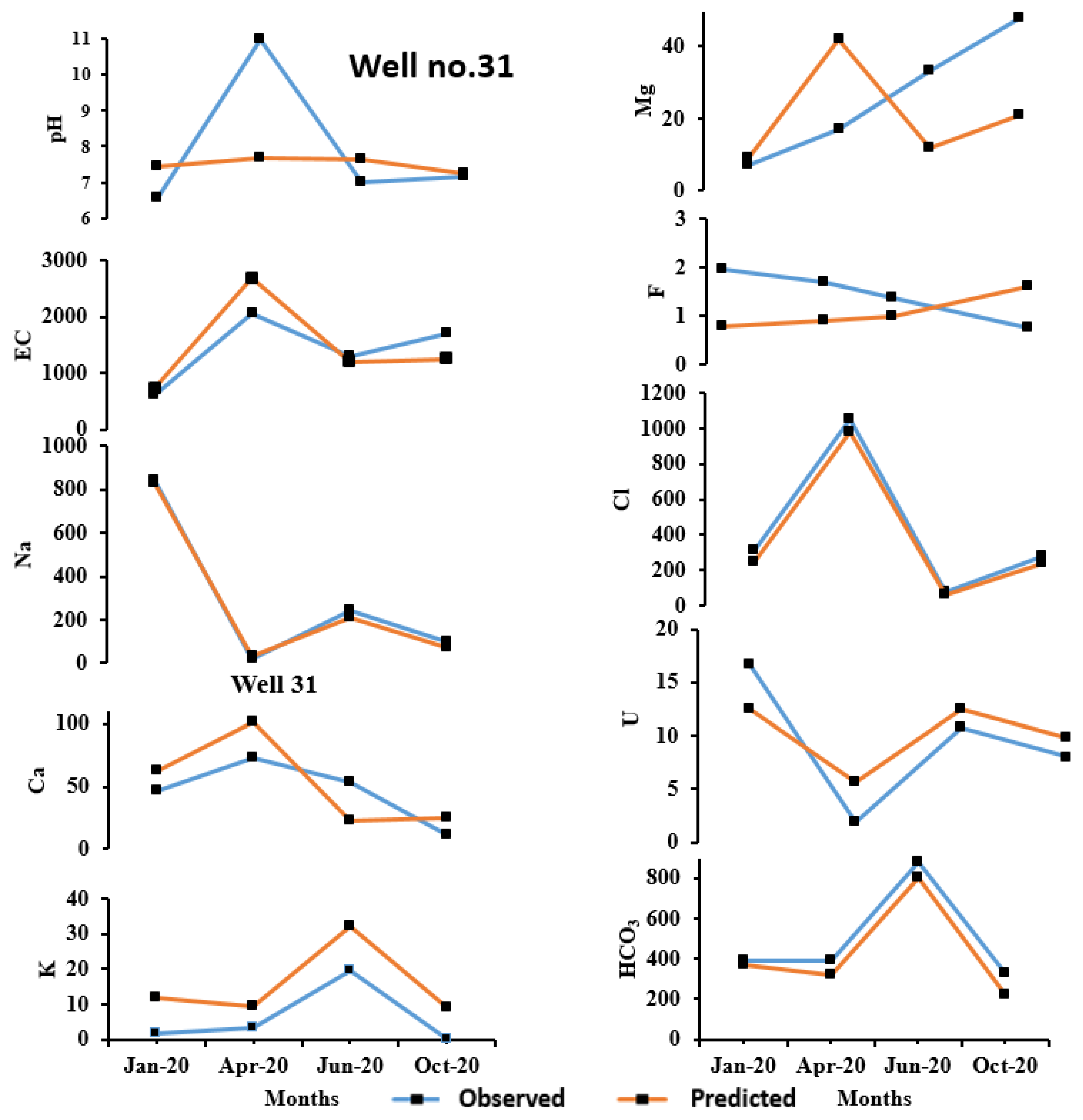
The temporal variation in the observed and predicted data for the period of validation during January 2020, April 2020, June 2020 and October 2020 are reasonably close to each other. As an example, the observed and predicted quality parameters of well no. 10 and well no. 31 are shown in Figure 6 and Figure 7, respectively. In well no. 10, except for F−, all other ions were predicted well. In well no. 31, except pH and F−, the observed and predicted concentrations all other ions are reasonably similar. Poor comparison between observed and predicted pH and F− is due to their low variance and standard deviation as compared to the other parameters. Furthermore, when the range of values is within a small limit, the prediction appears to be poor.
In order to study the temporal variation of predicted parameters in a closer scale, well no. 10 and well no. 31 were chosen (Figure 6 and Figure 7). It can be inferred that the prediction of F− and pH has great variation from the observed concentration. As discussed, this could be attributed to the range of parameter concentration and the variance. The ability of ACO-MLPNN to predict other parameters such as HCO3− and EC were analyzed, and Ca2+, Mg2+, Na+, K+, U2+ and Cl− were reasonably good.
3.3. Predicting Spatial Variation
The spatial variability of the predicted concentration of parameters was studied. The spatial distribution of the observed and predicted data for Na+ and Cl− for January 2020 are shown in Figure 8. The results are based on past data at a particular well. Thus, for every well, the model was built separately. The index variable for training the network is the “location of the well” and they lie in the same region. In reality, these wells might be connected, and groundwater may flow from one to the other. The network constructed by us does not consider the geological complexity of the region, which could be a drawback.
3.4. Performance Measures for ACO-MLPNN Model
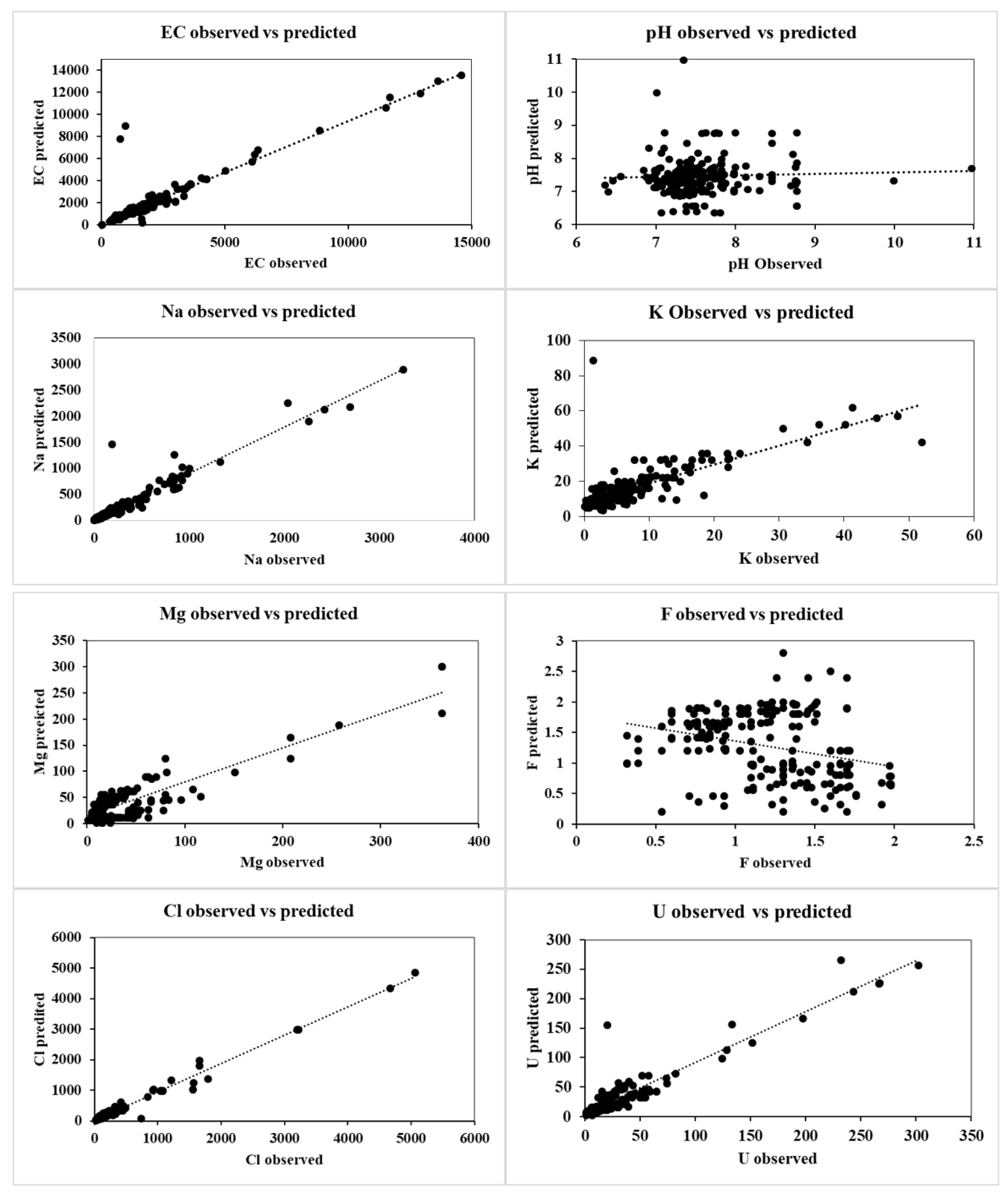
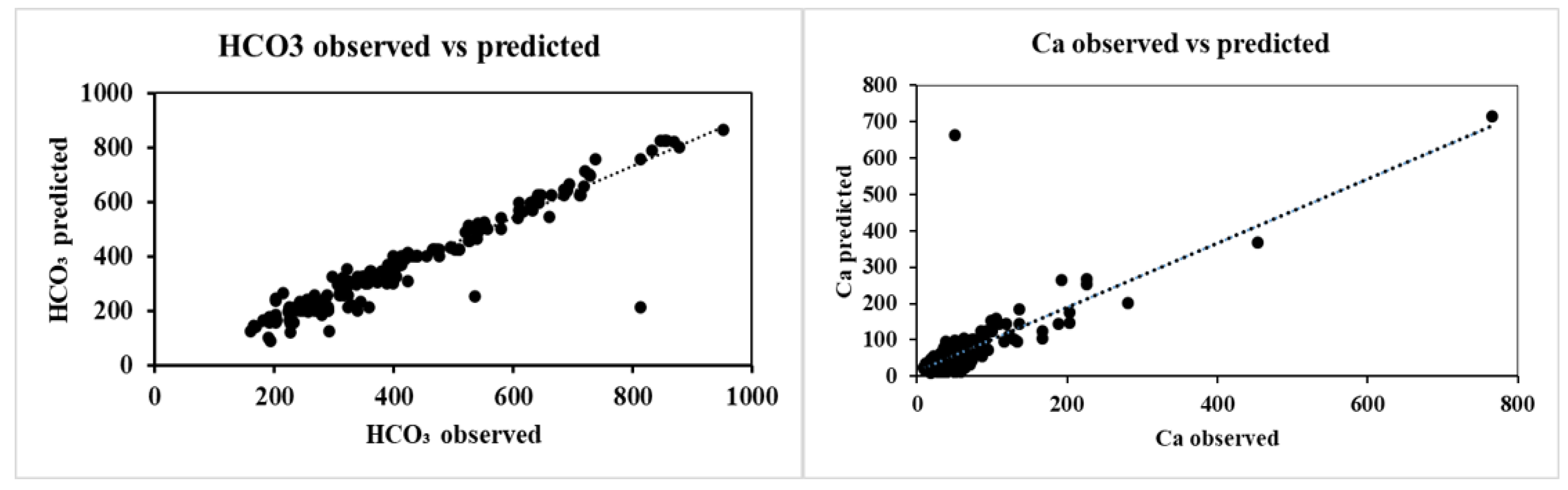
To quantify the error between the observed and predicted values, various performance efficiency parameters were used. R2, RMSE, NSE and MAE (Equations (3)–(6)) are the efficiency parameters that were chosen (Figure 3). The utilization of four statistical indices to evaluate the performance of the proposed model offers several advantages. Firstly, it ensures that the maximum error obtained during the evaluation process is within an acceptable range for a forecasting model. A linear correlation between the observed and predicted parameters are shown in Figure 9. Except for pH and F−, all other parameters are with reasonably good correlation (Figure 9).
The use of RMSE allows for a check on the sum of errors over the validation period, ensuring that it is not too high. Furthermore, the use of other indices provides a consistent level of errors, which is important in ensuring that the model’s performance is reliable when applied to unseen data in the testing period. Using multiple indices provides a more comprehensive evaluation of the model’s performance. Each index captures a different aspect of the model’s accuracy, and together they can give a more complete picture of the model’s strengths and weaknesses. In this way, the combined use of both R2, RMSE, NSE and MAE indices provides a great potential for maintaining a consistent level of error throughout the model evaluation process. Each error metric is unique and cannot be compared to another metric.
The range of R2 lies between 0 and 1, which describes the extent of dispersion in the predicted results. The major drawbacks of this method is that only dispersion is considered. Furthermore, over or under predictions cannot be determined from these error metrics. In the color palette presented in Figure 10, various error metrics chosen to evaluate the model performance are presented. According to R2, Cl−, Na+, U2+, HCO3−, Mg2+ and EC perform well. However, it is a generalized metric, and we cannot make a decision solely based on this alone. For RMSE and MAE, the errors are squared before they are averaged and hence, RMSE gives higher weightage to large errors as it increases with the variance of the frequency distribution of error magnitudes. Hence, RMSE has the tendency to be much larger than MAE and is very sensitive to outliers. RMSE is analogous to the standard deviation and focuses on the magnitude of errors. According to RMSE, K−, F− and U2+, good performance is displayed since the standard deviation for these parameters were considerably less. MAE, pH, K−, F−, U2+, Mg2+ and Ca+ also display good performance. NSE is commonly used to study the performance of hydrological models. NSE considers the mean value of the observed data and does not capture other skewness, variance etc. The metrics perform well for HCO3−, Cl− and pH.
These statistical indices represent the performance of the built ACO-MLPNN model for predicting various water quality parameters. Based on the given indices, the ACO-MLPNN model performed well for some parameters, such as NSE for pH, Cl− and HCO3− and R2 for Na+ and U2+. However, the model performance was not satisfactory for parameters, such as EC, Na+, K− based on NSE; and for EC and Na+, U2+, F− and Na+ based on RMSE. For pH, the R2 value is 0.04. This indicates that the model’s ability to predict depend on the variance in the data set; the RMSE value is 0.70, which indicates that the model’s average prediction error for pH is 0.99, indicating that the model’s predictions for pH are very close to the observed values, with only a small difference. Also, the MAE for pH is 0.53, indicating that the model’s predictions for pH are mostly accurate and have relatively low errors. Similarly, based on the results, the model performs well for some parameters such as Na+, Cl−, HCO3− and U2+ with relatively high R2 values and low RMSE and MAE values. However, the model performs poorly for some parameters such as EC, Ca2+, K− and Mg2+ with low R2 values and high RMSE and MAE values. In some cases, the NSE value is negative, indicating that the model performs lower than the mean value.
4. Conclusions
Machine learning models are being extensively used for classification, regression and prediction across different industries and applications. In the field of hydrogeology, they provide valuable insights into groundwater quality, allowing for effective management and protection of this critical resource. In order to study the efficiency of machine learning, an ant colony optimized multilayer perceptron neural network was used on a real groundwater quality dataset collected from northern Karnataka, India. We have explored the application of combination of ANN and ACO models to predict the groundwater quality. An MLPPNN-ACO model was used to predict the groundwater quality parameters with respect to time. This technique was used to predict the pH, EC, Na+, Ca+, Na+, K+, Mg2+, F−, Cl− and U+ of groundwater of 50 wells in the study area. A total of 500 models were built and it was observed that the prediction accuracy of these models is considerably good. In general, the models performed well when the standard deviation of the data was comparatively large. The MLPNN-ACO model learnt the data better when the standard deviation was higher. For such datasets, the model performance was considerably higher as indicated by the performance metrics. In the case of water quality parameters which did not vary much with respect to time such as pH, F− and U2+, the learning rate was poor. Furthermore, we evaluated the performance of the model by combining the predicted values of all the parameters at 50 locations at a particular time by preparing spatial contour maps. It was evident that the contour maps prepared using the model predicted values were comparable to the contour maps prepared using the observed data. The network suggested by us utilizes the ACO algorithm for optimizing ANN weights, but it requires careful experimentation and parameter tuning to achieve the best performance. However, this cannot replace sampling and analysis, and this will certainly help in reducing the temporal frequency of sample collection. Another major advantage is that we can constantly keep adding data as and when field data is available, and this will improve the model performance further. This technique can also be used in other domains which deal with multi-variant, spatial and temporal datasets. Though the ACO-MLPNN model may need further optimization and calibration to improve its performance for some parameters, in general, it predicted the temporal variation reasonably well for many parameters. Hence, the novel and robust ACO-MLPNN model developed by us can be used to predict groundwater quality of any region.
Author Contributions
R.B.—Conceptualization, Writing—original draft, Formal analysis, Software, validation, visualization, Methodology. L.E.—Supervision, Conceptualization, Writing—review & editing, Validation, Resources, Methodology. K.S.—Writing—review & editing, Validation. All authors have read and agreed to the published version of the manuscript.
Funding
This research received no external funding.
Informed Consent Statement
Not applicable.
Acknowledgments
The authors would like to thank Manoj Subramanian and Thirumurugan for water sampling and laboratory analysis from 2014 to 2016.
Conflicts of Interest
The authors declare no conflict of interest.
References
- Frank, M.R.; Wang, D.; Cebrian, M.; Rahwan, I. The evolution of citation graphs in artificial intelligence research. Nat. Mach. Intell. 2019, 1, 79–85. [Google Scholar] [CrossRef]
- Abiodun, O.I.; Jantan, A.; Omolara, A.E.; Dada, K.V.; Mohamed, N.A.; Arshad, H. State-of-the-art in artificial neural network applications: A survey. Heliyon 2018, 4, e00938. [Google Scholar] [CrossRef] [Green Version]
- Wang, D.; He, H.; Liu, D. Intelligent Optimal Control with Critic Learning for a Nonlinear Overhead Crane System. IEEE Trans. Ind. Inform. 2017, 14, 2932–2940. [Google Scholar] [CrossRef]
- Shahid, N.; Rappon, T.; Berta, W. Applications of artificial neural networks in health care organizational decision-making: A scoping review. PLoS ONE 2019, 14, e0212356. [Google Scholar] [CrossRef] [PubMed]
- Abhishek, K.; Singh, M.; Ghosh, S.; Anand, A. Weather Forecasting Model using Artificial Neural Network. Procedia Technol. 2012, 4, 311–318. [Google Scholar] [CrossRef] [Green Version]
- Selvamuthu, D.; Kumar, V.; Mishra, A. Indian stock market prediction using artificial neural networks on tick data. Financ. Innov. 2019, 5, 16. [Google Scholar] [CrossRef] [Green Version]
- Nandal, M.; Mor, N.; Sood, H. An Overview of Use of Artificial Neural Network in Sustainable Transport System. In Computational Methods and Data Engineering. Advances in Intelligent Systems and Computing; Singh, V., Asari, V., Kumar, S., Patel, R., Eds.; Springer: Singapore, 2021; Volume 1227. [Google Scholar] [CrossRef]
- Kujawa, S.; Niedbała, G. Artificial Neural Networks in Agriculture. Agriculture 2021, 11, 497. [Google Scholar] [CrossRef]
- Patel, J.; Goyal, J.L.P.A.R.K. Applications of Artificial Neural Networks in Medical Science. Curr. Clin. Pharmacol. 2007, 2, 217–226. [Google Scholar] [CrossRef] [PubMed]
- Okewu, E.; Adewole, P.; Misra, S.; Maskeliunas, R.; Damasevicius, R. Artificial Neural Networks for Educational Data Mining in Higher Education: A Systematic Literature Review. Appl. Artif. Intell. 2021, 35, 983–1021. [Google Scholar] [CrossRef]
- Srivastava, P.K.; Han, D.; Ramirez, M.R.; Islam, T. Machine Learning Techniques for Downscaling SMOS Satellite Soil Moisture Using MODIS Land Surface Temperature for Hydrological Application. Water Resour. Manag. 2013, 27, 3127–3144. [Google Scholar] [CrossRef]
- Maroufpoor, E.; Sanikhani, H.; Emamgholizadeh, S.; Kişi, Ö. Estimation of Wind Drift and Evaporation Losses from Sprinkler Irrigation systemS by Different Data-Driven Methods. Irrig. Drain. 2017, 67, 222–232. [Google Scholar] [CrossRef]
- Samadianfard, S.; Sattari, M.T.; Kisi, O.; Kazemi, H. Determining Flow Friction Factor in Irrigation Pipes Using Data Mining and Artificial Intelligence Approaches. Appl. Artif. Intell. 2014, 28, 793–813. [Google Scholar] [CrossRef]
- Alagha, J.S.; Seyam, M.; Said, A.; Mogheir, Y. Integrating an artificial intelligence approach with k-means clustering to model groundwater salinity: The case of Gaza coastal aquifer (Palestine). Hydrogeol. J. 2017, 25, 2347–2361. [Google Scholar] [CrossRef]
- Nourani, V.; Mousavi, S.; Sadikoglu, F. Conjunction of artificial intelligence-meshless methods for contaminant transport modeling in porous media: An experimental case study. J. Hydroinformatics 2017, 20, 1163–1179. [Google Scholar] [CrossRef] [Green Version]
- Khaki, M.; Yusoff, I.; Islami, N. Application of the Artificial Neural Network and Neuro-fuzzy System for Assessment of Groundwater Quality. CLEAN–Soil Air Water 2014, 43, 551–560. [Google Scholar] [CrossRef]
- Kulisz, M.; Kujawska, J.; Przysucha, B.; Cel, W. Forecasting Water Quality Index in Groundwater Using Artificial Neural Network. Energies 2021, 14, 5875. [Google Scholar] [CrossRef]
- Nordin, N.F.C.; Mohd, N.S.; Koting, S.; Ismail, Z.; Sherif, M.; El-Shafie, A. Groundwater quality forecasting modelling using artificial intelligence: A review. Groundw. Sustain. Dev. 2021, 14, 100643. [Google Scholar] [CrossRef]
- Jackson, E.K.; Roberts, W.; Nelsen, B.; Williams, G.P.; Nelson, E.J.; Ames, D.P. Introductory overview: Error metrics for hydrologic modelling—A review of common practices and an open source library to facilitate use and adoption. Environ. Model. Softw. 2019, 119, 32–48. [Google Scholar] [CrossRef]
- Ubah, J.I.; Orakwe, L.C.; Ogbu, K.N.; Awu, J.I.; Ahaneku, I.E.; Chukwuma, E.C. Forecasting water quality parameters using artificial neural network for irrigation purposes. Sci. Rep. 2021, 11, 24438. [Google Scholar] [CrossRef] [PubMed]
- Mustafa, M.R.; Rezaur, R.B.; Saiedi, S.; Isa, M.H. River Suspended Sediment Prediction Using Various Multilayer Perceptron Neural Network Training Algorithms—A Case Study in Malaysia. Water Resour. Manag. 2012, 26, 1879–1897. [Google Scholar] [CrossRef]
- Ghumman, A.; Ghazaw, Y.M.; Sohail, A.; Watanabe, K. Runoff forecasting by artificial neural network and conventional model. Alex. Eng. J. 2011, 50, 345–350. [Google Scholar] [CrossRef] [Green Version]
- Shiri, J.; Kisi, O.; Yoon, H.; Lee, K.-K.; Nazemi, A.H. Predicting groundwater level fluctuations with meteorological effect implications—A comparative study among soft computing techniques. Comput. Geosci. 2013, 56, 32–44. [Google Scholar] [CrossRef]
- Nazari, S.; Momtaz, H.R.; Servati, M. Modeling cation exchange capacity in gypsiferous soils using hybrid approach involving the artificial neural networks and ant colony optimization (ANN–ACO). Model. Earth Syst. Environ. 2022, 8, 4065–4074. [Google Scholar] [CrossRef]
- Haghiabi, A.H.; Nasrolahi, A.H.; Parsaie, A. Water quality prediction using machine learning methods. Water Qual. Res. J. 2018, 53, 3–13. [Google Scholar] [CrossRef]
- Aldhyani, T.H.H.; Al-Yaari, M.; Alkahtani, H.; Maashi, M. Water Quality Prediction Using Artificial Intelligence Algorithms. Appl. Bionics Biomech. 2020, 2020, 6659314. [Google Scholar] [CrossRef]
- Lu, H.; Ma, X. Hybrid decision tree-based machine learning models for short-term water quality prediction. Chemosphere 2020, 249, 126169. [Google Scholar] [CrossRef]
- Nayan, A.-A.; Kibria, M.G.; Rahman, M.O.; Saha, J. River Water Quality Analysis and Prediction Using GBM. In Proceedings of the 2020 2nd International Conference on Advanced Information and Communication Technology (ICAICT), Dhaka, Bangladesh, 28–29 November 2020; pp. 219–224. [Google Scholar] [CrossRef]
- Shen, C. A Transdisciplinary Review of Deep Learning Research and Its Relevance for Water Resources Scientists. Water Resour. Res. 2018, 54, 8558–8593. [Google Scholar] [CrossRef]
- Afshar, A.; Massoumi, F.; Afshar, A.; Mariño, M.A. State of the Art Review of Ant Colony Optimization Applications in Water Resource Management. Water Resour. Manag. 2015, 29, 3891–3904. [Google Scholar] [CrossRef]
- Bhavya, R.; Elango, L. Ant-Inspired Metaheuristic Algorithms for Combinatorial Optimization Problems in Water Resources Management. Water 2023, 15, 1712. [Google Scholar] [CrossRef]
- Bagheri, M.; Mirbagheri, S.A.; Bagheri, Z.; Kamarkhani, A.M. Modeling and optimization of activated sludge bulking for a real wastewater treatment plant using hybrid artificial neural networks-genetic algorithm approach. Process. Saf. Environ. Prot. 2015, 95, 12–25. [Google Scholar] [CrossRef]
- Lu, W.Z.; Fan, H.Y.; Lo, S.M. Application of evolutionary neural network method in predicting pollutant levels in downtown area of Hong Kong. Neurocomputing 2003, 51, 387–400. [Google Scholar] [CrossRef]
- Liu, Y.; Zhu, Q.; Yao, D.; Xu, W. Forecasting Urban Air Quality via a Back-Propagation Neural Network and a Selection Sample Rule. Atmosphere 2015, 6, 891–907. [Google Scholar] [CrossRef] [Green Version]
- Da, Y.; Xiurun, G. An improved PSO-based ANN with simulated annealing technique. Neurocomputing 2005, 63, 527–533. [Google Scholar] [CrossRef]
- Chau, K. Application of a PSO-based neural network in analysis of outcomes of construction claims. Autom. Constr. 2007, 16, 642–646. [Google Scholar] [CrossRef] [Green Version]
- Groundwater Quality in Shallow Aquifers in INDIA, CGWB Report 2018. Available online: http://cgwb.gov.in/WQ/Ground%20Water%20Book-F.pdf (accessed on 1 June 2019).
- Carrard, N.; Foster, T.; Willetts, J. Groundwater as a Source of Drinking Water in Southeast Asia and the Pacific: A Multi-Country Review of Current Reliance and Resource Concerns. Water 2019, 11, 1605. [Google Scholar] [CrossRef] [Green Version]
- Motagh, M.; Shamshiri, R.; Haghshenas Haghighi, M.; Wetzel, H.-U.; Akbari, B.; Nahavandchi, H.; Roessner, S.; Arabi, S. Quantifying groundwater exploitation induced subsidence in the Rafsanjan plain, southeastern Iran, using InSAR time-series and in situ measurements. Eng. Geol. 2017, 218, 134–151. [Google Scholar] [CrossRef]
- Gorelick, S.M.; Zheng, C. Global change and the groundwater management challenge. Water Resour. Res. 2015, 51, 3031–3051. [Google Scholar] [CrossRef]
- Sinha, D.; Prasad, P. Health effects inflicted by chronic low-level arsenic contamination in groundwater: A global public health challenge. J. Appl. Toxicol. 2020, 40, 87–131. [Google Scholar] [CrossRef] [PubMed]
- Chakraborti, D.; Rahman, M.M.; Das, B.; Chatterjee, A.; Das, D.; Nayak, B.; Pal, A.; Chowdhury, U.K.; Ahmed, S.; Biswas, B.K.; et al. Groundwater arsenic contamination and its health effects in India. Hydrogeol. J. 2017, 25, 1165–1181. [Google Scholar] [CrossRef]
- Shaji, E.; Santosh, M.; Sarath, K.; Prakash, P.; Deepchand, V.; Divya, B. Arsenic contamination of groundwater: A global synopsis with focus on the Indian Peninsula. Geosci. Front. 2020, 12, 101079. [Google Scholar] [CrossRef]
- Sappa, G.; Ergul, S.; Ferranti, F. Geochemical modeling and multivariate statistical evaluation of trace elements in arsenic contaminated groundwater systems of Viterbo Area, (Central Italy). SpringerPlus 2014, 3, 237. [Google Scholar] [CrossRef] [Green Version]
- Karangoda, R.; Nanayakkara, K. Use of the water quality index and multivariate analysis to assess groundwater quality for drinking purpose in Ratnapura district, Sri Lanka. Groundw. Sustain. Dev. 2023, 21, 100910. [Google Scholar] [CrossRef]
- May, R.J.; Maier, H.R.; Dandy, G.C. Developing Artificial Neural Networks for Water Quality Modelling and Analysis. In Modelling of Pollutants in Complex Environmental Systems; Hanrahan, G., Ed.; ILM Publications: St. Albans, UK, 2009. [Google Scholar]
- Barzegar, R.; Adamowski, J.; Moghaddam, A.A. Application of wavelet-artificial intelligence hybrid models for water quality prediction: A case study in Aji-Chay River, Iran. Stoch. Environ. Res. Risk Assess. 2016, 30, 1797–1819. [Google Scholar] [CrossRef]
- Wong, Y.J.; Shimizu, Y.; Kamiya, A.; Maneechot, L.; Bharambe, K.P.; Fong, C.S.; Sulaiman, N.M.N. Application of artificial intelligence methods for monsoonal river classification in Selangor river basin, Malaysia. Environ. Monit. Assess. 2021, 193, 438. [Google Scholar] [CrossRef]
- Sakizadeh, M. Artificial intelligence for the prediction of water quality index in groundwater systems. Model. Earth Syst. Environ. 2016, 2, 8. [Google Scholar] [CrossRef]
- Ahmed, A.N.; Othman, F.B.; Afan, H.A.; Ibrahim, R.K.; Fai, C.M.; Hossain, S.; Ehteram, M.; Elshafie, A. Machine learning methods for better water quality prediction. J. Hydrol. 2019, 578, 124084. [Google Scholar] [CrossRef]
- Saghi-Jadid, M.; Ketabchi, H. Restoration management of groundwater resources using the combined model of numerical simulation—Evolutionary ant colony optimization. Iran-Water Resour. Res. 2019, 15, 119–133. [Google Scholar]
- Ketabchi, H.; Ataie-Ashtiani, B. Evolutionary algorithms for the optimal management of coastal groundwater: A comparative study toward future challenges. J. Hydrol. 2015, 520, 193–213. [Google Scholar] [CrossRef]
- Mohammadhassani, J.; Dadvand, A.; Khalilarya, S.; Solimanpur, M. Prediction and reduction of diesel engine emissions using a combined ANN–ACO method. Appl. Soft Comput. 2015, 34, 139–150. [Google Scholar] [CrossRef]
- Tehrani, R.; Khodayar, F. Optimization of the Artificial Neural Networks Using Ant Colony Algorithm to Predict the Variation of Stock Price Index. J. Appl. Sci. 2010, 10, 221–225. [Google Scholar] [CrossRef]
- Lefnaoui, S.; Rebouh, S.; Bouhedda, M.; Yahoum, M.M. ANN Optimization Using Ant Colony Algorithm for Predicting the Valsartan Sustained Release from Polyelectrolyte Complexes Matrix Tablets. In Proceedings of the 2019 International Conference on Applied Automation and Industrial Diagnostics (ICAAID), Elazig, Turkey, 25–27 September 2019; pp. 1–6. [Google Scholar] [CrossRef]
- Saghatforoush, A.; Monjezi, M.; Faradonbeh, R.S.; Armaghani, D.J. Combination of neural network and ant colony optimization algorithms for prediction and optimization of flyrock and back-break induced by blasting. Eng. Comput. 2015, 32, 255–266. [Google Scholar] [CrossRef]
- Dorigo, M.; Maniezzo, V.; Colorni, A. Ant System: An Autocatalytic Optimizing Process; Technical Report 91-016; Politecnico di Milano: Milan, Italy, 1991. [Google Scholar]
- Mavrovouniotis, M.; Yang, S. Evolving neural networks using ant colony optimization with pheromone trail limits. IEEE 2013, 13, 16–23. [Google Scholar] [CrossRef]
- Kumar, P.; Lai, S.H.; Mohd, N.S.; Kamal, R.; Ahmed, A.N.; Sherif, M.; Sefelnasr, A.; El-Shafie, A. Enhancement of nitrogen prediction accuracy through a new hybrid model using ant colony optimization and an Elman neural network. Eng. Appl. Comput. Fluid Mech. 2021, 15, 1843–1867. [Google Scholar] [CrossRef]
- Zhang, H.; Nguyen, H.; Bui, X.-N.; Nguyen-Thoi, T.; Bui, T.-T.; Nguyen, N.; Vu, D.-A.; Mahesh, V.; Moayedi, H. Developing a novel artificial intelligence model to estimate the capital cost of mining projects using deep neural network-based ant colony optimization algorithm. Resour. Policy 2020, 66, 101604. [Google Scholar] [CrossRef]
- Khajeh, M.; Hezaryan, S. Combination of ACO-artificial neural network method for modeling of manganese and cobalt extraction onto nanometer SiO2 from water samples. J. Ind. Eng. Chem. 2013, 19, 2100–2107. [Google Scholar] [CrossRef]
- Jayaprakash, A.; KeziSelvaVijila, C. Feature selection using Ant Colony Optimization (ACO) and Road Sign Detection and Recognition (RSDR) system. Cogn. Syst. Res. 2019, 58, 123–133. [Google Scholar] [CrossRef]
- Van Rossum, G. Python Reference Manual; Department of Computer Science [CS] at CWI: Nampa, ID, USA, 1995. [Google Scholar]
- Bowden, G.J.; Maier, H.R.; Dandy, G.C. Optimal division of data for neural network models in water resources applications. Water Resour. Res. 2002, 38, 2-1–2-11. [Google Scholar] [CrossRef] [Green Version]
- Krause, P.; Boyle, D.P.; Bäse, F. Comparison of different efficiency criteria for hydrological model assessment. Adv. Geosci. 2005, 5, 89–97. [Google Scholar] [CrossRef] [Green Version]
- Manoj, S.; Thirumurugan, M.; Elango, L. An integrated approach for assessment of groundwater quality in and around uranium mineralized zone, Gogi region, Karnataka, India. Arab. J. Geosci. 2017, 10, 557. [Google Scholar] [CrossRef]
- Bhavya, R.; Sivaraj, K.; Elango, L. Assessing the Baseline Uranium in Groundwater around a Proposed Uraninite Mine and Identification of a Nearby New Reserve. Minerals 2023, 13, 157. [Google Scholar] [CrossRef]
- Manoj, S. Distribution of Uranium in Soils and Rocks and its Impact on Surface Water and Groundwater Quality in Uranium Mineralised Region. Shahapur Taluk, Karnataka, India. Thesis Completed. 2018. Available online: https://scholar.google.com.hk/scholar?hl=zh-CN&as_sdt=0%2C5&q=Distribution+of+Uranium+in+Soils+and+Rocks+and+its+Impact+on+Surface+Water+and+Groundwater+Quality+in+Uranium+Mineralised+Region&btnG= (accessed on 2 May 2023).
- Lakshmanan, E.; Kannan, R.; Kumar, M.S. Major ion chemistry and identification of hydrogeochemical processes of ground water in a part of Kancheepuram district, Tamil Nadu, India. Environ. Geosci. 2003, 10, 157–166. [Google Scholar] [CrossRef]
- Westfall, P.H. Kurtosis as Peakedness, 1905–2014. R.I.P. Am. Stat. 2014, 68, 191–195. [Google Scholar] [CrossRef] [PubMed] [Green Version]
Figure 1.
Algorithmic frame for the ACO algorithm for weight optimization.

Figure 2.
Workflow of ACO-MLPNN for prediction of groundwater quality parameters.

Figure 3.
Structure of the proposed ACO-MLPNN model.

Figure 4.
Location of the study site and monitoring wells.

Figure 5.
Time series of groundwater quality parameters with red lines indicating the commencement of testing period.
Figure 5.
Time series of groundwater quality parameters with red lines indicating the commencement of testing period.


Figure 6.
Temporal variation of observed and predicted pH, EC, Na+, Ca+, Na+, K+, Mg2+, F−, Cl− and U+ in well 10.
Figure 6.
Temporal variation of observed and predicted pH, EC, Na+, Ca+, Na+, K+, Mg2+, F−, Cl− and U+ in well 10.

Figure 7.
Temporal variation of observed and predicted pH, EC, Na+, Ca+, Na+, K+, Mg2+, F−, Cl− and U+ in well 31.
Figure 7.
Temporal variation of observed and predicted pH, EC, Na+, Ca+, Na+, K+, Mg2+, F−, Cl− and U+ in well 31.

Figure 8.
Spatial variation of (i) observed Cl− concentration, (ii) predicted Cl− concentration, (iii) Observed Na+ concentration, and (iv) predicted Na+ concentration.
Figure 8.
Spatial variation of (i) observed Cl− concentration, (ii) predicted Cl− concentration, (iii) Observed Na+ concentration, and (iv) predicted Na+ concentration.

Figure 9.
Linear correlation between observed and predicted concentrations of quality parameters for all the wells in 2020.
Figure 9.
Linear correlation between observed and predicted concentrations of quality parameters for all the wells in 2020.


Figure 10.
Performance of the 500 (50 locations and 10 parameters) models based on the 4 metrics. Notes: R2: values range from 0 to 1, where a value closer to 0 indicates lesser fit, and a value closer to 1 indicates better fit; RMSE: a lower RMSE value indicates a better fit, and a higher RMSE value indicates a poorer fit; NSE: a value ranges from negative infinity to 1, where 1 indicates a perfect match, and 0 indicates that predictions are no better than the mean of the observed data, whereas negative value indicates that predictions are worse than using the mean of the observed data, and a value greater than 0.5 is considered to be a good fit; MAE: a lower MAE value indicates a better fit, and a higher MAE value indicates a poorer fit.


Table 1.
Months of sample collection and periods used for training, testing and validation.
| Months | Training Data | Testing Data | Validation Data | |||
|---|---|---|---|---|---|---|
| 2014 | 2015 | 2016 | 2018 | 2019 | 2020 | |
| January | * | * | * | |||
| February | * | |||||
| March | * | |||||
| April | * | |||||
| May | * | |||||
| June | * | * | * | |||
| August | * | |||||
| September | * | * | * | |||
| October | * | * | ||||
| December | * | |||||
Note: * indicates field visit for sample collection.
Table 2.
Descriptive statistics of groundwater physicochemical parameters.
| Parameter | Units | Mean | Standard Deviation | Variance | Kurtosis | Skewness | Minimum | Maximum |
|---|---|---|---|---|---|---|---|---|
| pH | - | - | 7.41 | 54.85 | 4.81 | 2.31 | 6.36 | 10.97 |
| EC | μS/cm | 2227.78 | 2464.82 | 6,075,317.81 | 12.26 | 3.35 | 27.90 | 15,560.00 |
| Ca | mg/L | 87.39 | 91.29 | 8334.71 | 12.64 | 3.27 | 9.70 | 765.30 |
| Na | mg/L | 270.70 | 441.80 | 195,188.01 | 15.43 | 3.76 | 2.39 | 3246.00 |
| K | mg/L | 7.31 | 7.42 | 55.05 | 7.62 | 2.31 | 0.02 | 52.00 |
| Mg | mg/L | 57.43 | 76.39 | 5835.21 | 13.82 | 3.48 | 0.00 | 505.00 |
| F | mg/L | 1.20 | 0.61 | 0.37 | 7.44 | 1.67 | 0.10 | 5.80 |
| Cl | mg/L | 400.79 | 777.55 | 604,584.95 | 18.71 | 4.18 | 25.68 | 5083.00 |
| U | mg/L | 26.28 | 41.98 | 1762.72 | 17.71 | 3.91 | 0.07 | 302.00 |
| HCO3 | mg/L | 411.76 | 180.01 | 32,402.67 | 0.05 | 0.87 | 143.22 | 956.99 |
Disclaimer/Publisher’s Note: The statements, opinions and data contained in all publications are solely those of the individual author(s) and contributor(s) and not of MDPI and/or the editor(s). MDPI and/or the editor(s) disclaim responsibility for any injury to people or property resulting from any ideas, methods, instructions or products referred to in the content. |
© 2023 by the authors. Licensee MDPI, Basel, Switzerland. This article is an open access article distributed under the terms and conditions of the Creative Commons Attribution (CC BY) license (https://creativecommons.org/licenses/by/4.0/).
Share and Cite
MDPI and ACS Style
Bhavya, R.; Sivaraj, K.; Elango, L. Ant Colony Based Artificial Neural Network for Predicting Spatial and Temporal Variation in Groundwater Quality. Water 2023, 15, 2222. https://doi.org/10.3390/w15122222
AMA Style
Bhavya R, Sivaraj K, Elango L. Ant Colony Based Artificial Neural Network for Predicting Spatial and Temporal Variation in Groundwater Quality. Water. 2023; 15(12):2222. https://doi.org/10.3390/w15122222
Chicago/Turabian StyleBhavya, Ravinder, Kaveri Sivaraj, and Lakshmanan Elango. 2023. "Ant Colony Based Artificial Neural Network for Predicting Spatial and Temporal Variation in Groundwater Quality" Water 15, no. 12: 2222. https://doi.org/10.3390/w15122222
Note that from the first issue of 2016, this journal uses article numbers instead of page numbers. See further details here.