Measuring Groundwater Flow Velocities near Drinking Water Extraction Wells in Unconsolidated Sediments

Abstract

Groundwater is an important source of drinking water in coastal regions with predominantly unconsolidated sediments. To protect and manage drinking water extraction wells in these regions, reliable estimates of groundwater flow velocities around well fields are of paramount importance. Such measurements help to identify the dynamics of the groundwater flow and its response to stresses, to optimize water resources management, and to calibrate groundwater flow models. In this article, we review approaches for measuring the relatively high groundwater flow velocity measurements near these wells. We discuss and review their potential and limitations for use in this environment. Environmental tracer measurements are found to be useful for regional scale estimates of groundwater flow velocities and directions, but their use is limited near drinking water extraction wells. Surface-based hydrogeophysical measurements can potentially provide insight into groundwater flow velocity patterns, although the depth is limited in large-scale measurement setups. Active-heating distributed temperature sensing (AH-DTS) provides direct measurements of in situ groundwater flow velocities and can monitor fluctuations in the high groundwater flow velocities near drinking water extraction wells. Combining geoelectrical measurements with AH-DTS shows the potential to estimate a 3D groundwater flow velocity distribution to fully identify groundwater flow towards drinking water extraction wells.

1. Introduction

Globally, groundwater serves as an important source for drinking water, particularly in coastal regions where unconsolidated sedimentary aquifers occur [1]. Increasing groundwater extraction and the increasing use of the subsurface, such as aquifer thermal energy storage [2], result in a higher potential for interference; requiring better identification and monitoring of groundwater flow to enable the sustainable use of fresh groundwater [3]. To effectively protect and manage drinking water extraction wells, a sound understanding of groundwater flow velocity (magnitude and direction) is of paramount importance.

Apart from providing better insight into the groundwater flow dynamics around drinking water extraction wells, velocity measurements help to determine the origin of the extracted groundwater or to locate well clogging zones along the well filter. Furthermore, velocity measurements can be used to better constrain groundwater models, in addition to piezometric data. The paucity of hydraulic head measurements and the fact that they do not directly inform about groundwater flow magnitudes without a detailed characterization of hydraulic properties (conductivity and storage) generally results in simplified numerical models that include large-scale homogeneous layers, in which local fine-scaled heterogeneity is not represented [4]. This may result in groundwater flow velocity estimates with large uncertainties, especially at the local scale, such as in the vicinity of a drinking water extraction well field [5]. Efforts to map local heterogeneity on a meter scale are needed to provide ideal input for detailed hydrogeological modeling near a drinking water extraction field [5]. The joint use of groundwater head and velocity measurements provides direct insight into fine-scale heterogeneity, which subsequently allows for better calibration, making fine-scale modeling possible for analyzing local groundwater flow around drinking water extraction wells.

Groundwater measurement techniques typically focus on aquifer characteristics (e.g., hydraulic conductivity and storage), the potential state of the groundwater system (hydraulic head), quality, age, and flow velocities. There are several excellent reviews regarding available techniques to measure groundwater flow velocities focused on specific types of measurement or fields of interest. For instance, Kaufman and Orlob [6] and Evans [7] provide reviews on the use of solute tracers to estimate groundwater flow. More recent reviews are those by Bethke and Johnson [8] and Chambers et al. [9] on the use of environmental tracers to estimate groundwater residence time. Cartwright et al. [10] focus on techniques to asses groundwater recharge, while Anderson [11], and more recently, Kurylyk et al. [12], advocate and discuss the general application of using heat as a groundwater tracer. Other reviews relevant to groundwater flow velocity measurements include those by Revil et al. [13] on the use of geoelectrical methods for the characterization and monitoring of groundwater flow and by Bense et al. [14] on measuring groundwater temperatures using fiber-optic cables in groundwater boreholes.

However, there are specific restrictions in the use of the abovementioned techniques when measuring groundwater flow velocity near drinking water extraction wells. This calls for a review of the techniques that can operate within these restrictions, as the need for measuring groundwater flow velocities near drinking water extraction wells is increasing. The main concern of drinking water companies is to protect the water quality of the groundwater near their wells. Thus, the companies are not willing to use solutes as tracers. In the Netherlands, for example, the introduction of solutes is even prohibited or limited by law. Furthermore, the potential of natural tracers is often limited because drinking water extraction wells are located at sites where groundwater quality has to be as optimal as possible, meaning the presence of natural tracers is often limited. Here, we provide a review of field techniques to measure groundwater flow velocity near drinking water extraction wells located in unconsolidated sedimentary aquifer systems that operate within these limits. Our review (1) provides an overview of the measurement techniques that can be applied within the restrictions around drinking water extraction wells, (2) addresses the specific potential and limitations of these techniques in a well field setup, (3) provides references to more detailed information on the mentioned techniques, as well as recent applications, and (4) identifies the unexplored potential of combining measurement techniques. The groundwater flow velocity measurement techniques are classified into tracer measurements and geophysical measurements.

2. Tracer Measurements

Field experiments using environmental tracers (a natural present or introduced chemical substance) track the movement of that tracer to estimate groundwater flow and transport properties of porous media. For contaminant transport, the estimation of sorption and hydrodynamic dispersion in the subsurface environment using tracers is also of interest [15]. Groundwater flow velocity and direction can also be investigated using tracer experiments.

By following the center of mass of a tracer, the advective velocity can be directly related to groundwater flow velocities (Darcy velocity: L T-1).

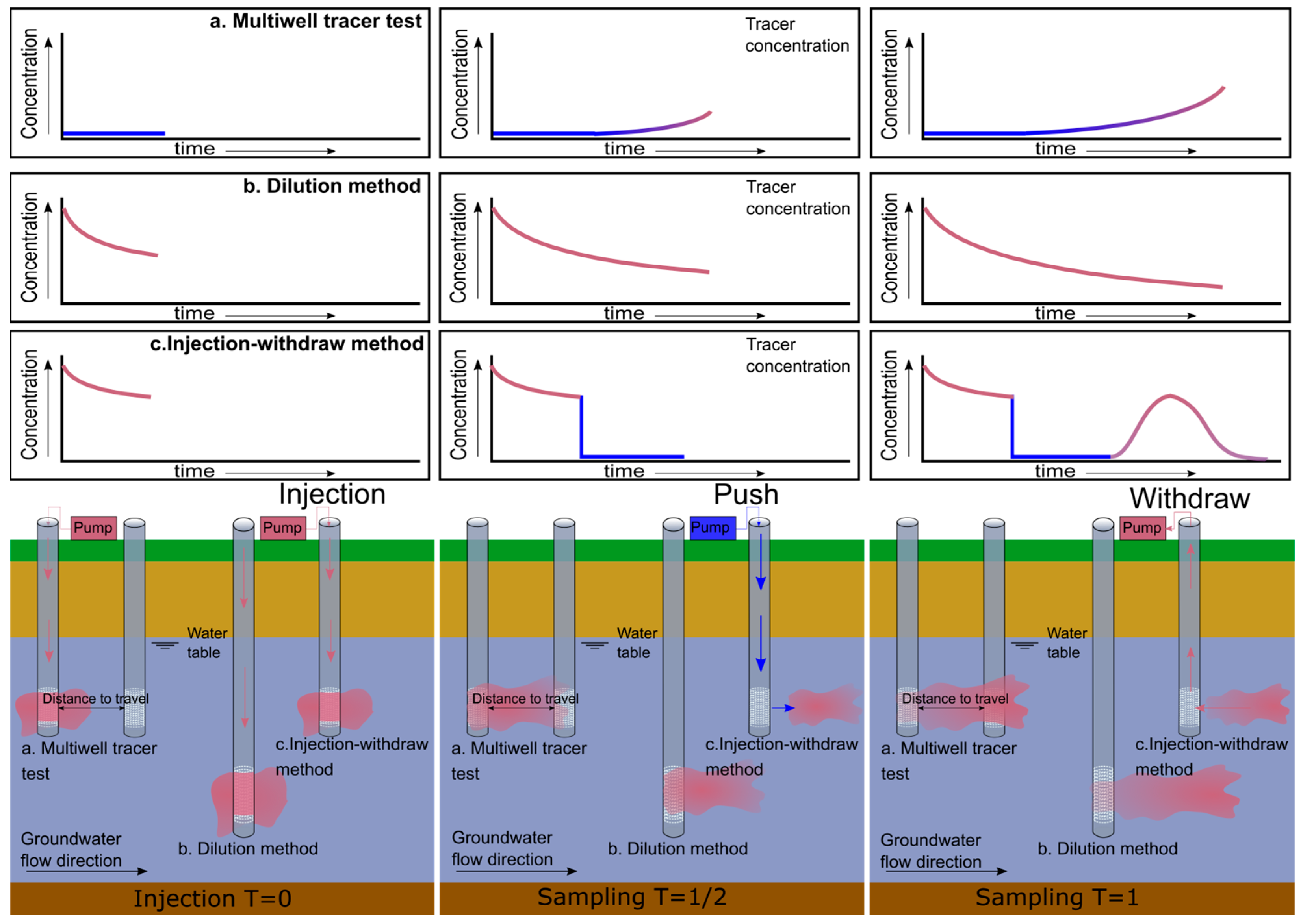
Various configurations of multi-well tracer measurements are used for simple tracer measurements (Figure 1a). An injection well is used where tracers are either actively injected, or allowed to passively enter the groundwater flow path. The time it takes to travel a certain distance from the injection point to an observation well is used to calculate the groundwater flow velocity. However, subsurface solute transport is not only controlled by groundwater flow (advection), but also by mechanical dispersion and molecular diffusion, as well as by absorption/retardation and decay [16]. In addition, variable density or dynamic viscosity due to temperature or solute gradients can influence effective hydraulic conductivity and therefore, groundwater flow. These processes need to be significantly small, or incorporated into the analyses, to obtain a realistic estimate of the natural groundwater flow velocity [17,18].

In our review, we distinguish between artificial and environmental tracers and recognize the specific potential of using temperature as a tracer for use near drinking water extraction wells. In Appendix A, an overview of the relevant literature regarding tracer measurement techniques is provided.

2.1. Artifical Tracer Measurements

Artificial tracers are elements such as dyes, radioactive isotopes, or detergents that are introduced into the environment [19]. Appendix B provides an overview of the relevant literature regarding commonly used artificial tracers. Artificial tracer measurements can be translated to groundwater flow velocity magnitude or direction, depending on the measurement setup. Setups using single or multiple wells, both passively or with active pumping and injection, are commonly used techniques. Figure 1 shows typical field setups for tracer measurements.

The single-well dilution method introduces a tracer into a well, without active pumping, to force the tracer into the well (Figure 1b). The dilution of the tracer in the well itself is monitored over time, which is related to the natural horizontal groundwater flow [16]. For the interpretation of the results, the distortion of the flow by the well must be known [20,21]. The dilution method is easy to apply in wells (both cased or uncased). Parts of the well screen are compartmentalized using packers to perform the test at different depths in order to obtain vertical profiles of the groundwater flow velocity. The challenge in applying the dilution method is separating the vertical and horizontal flow components, thereby identifying sections of vertical flow in the well and excluding them from the calculation of the horizontal flow [22]. Vertical flow over an aquitard can occur when two filters are placed in separate aquifers with different hydraulic pressures, resulting in a crossflow through the well in a vertical direction.

The injection–withdrawal (push–pull) method (Figure 1c) is an active version of the passive dilution test described above. The tracer is injected using excess pressure in the wellhead, allowing it to travel out of the well, with the additional influence of the natural groundwater flow, for a known period of time. After this period, the tracer is recovered by pumping the well at a constant rate. The shape of the breakthrough curve during recovery can be related to the groundwater flow velocity [23].

More interpretation methods are developed based on these principles. The finite volume point dilution method (FVPDM) uses a controlled and continuously injection of the tracer into a well, and it is further developed to monitor groundwater flux over time [24]. The passive flux meter (PFM) holds the potential for measuring water and contaminant fluxes [25]. The PFM containing a resident tracer evenly distributed over a sorptive matrix and is exposed to groundwater flow by its placement into a well. The displacement of the tracer in the matrix by the passing groundwater can be related to the flow [15]. The In-Well Point Velocity Probe (IWPVP) is designed is such a way that a measurable velocity is obtained that can be related to the natural groundwater flow outside of the well. In the chamber located at the center of the probe, a tracer is released. In detection channels from this chamber towards the outside of the probe, the tracer concentration is tracked [26].

The use of an artificial tracer for measuring groundwater flow near drinking water extraction wells is in most cases, not an option. The use of artificial tracers is often restricted near drinking water extraction wells to protect the quality of the water. One exception is the use of temperature as a tracer, as it holds no direct risk for the water quality. Even if restrictions allow for the use of tracers in small concentrations, application in the direct vicinity of an operating well (within ~20 m distance, depending on the occurring groundwater flow velocities) can be extremely challenging, especially in regards to multi-well setups. Moreover, high dilution rates due to the high flow velocities would require the injection of relatively large quantities of the tracer, as the use of smaller quantities makes the detection of the tracer challenging.

2.2. Artifical Temperature Tracer Measurements

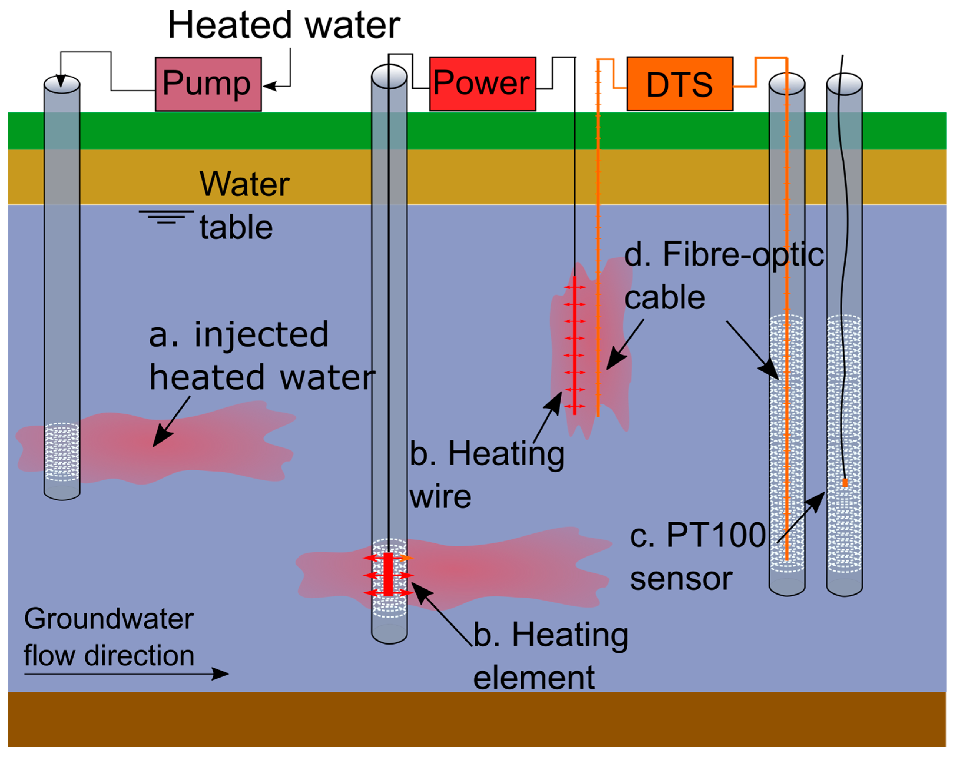
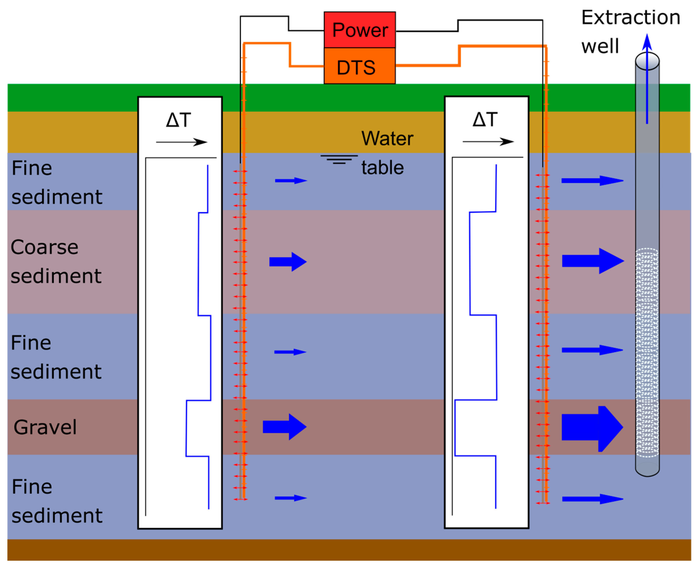
Introducing heat as a tracer does not significantly affect the groundwater quality and can therefore be applied without restrictions near drinking water extraction wells. The application of heat as an artificial tracer entails the capture of induced temperature differences. A temperature difference is realized by (a) injecting water (Figure 2a) with a contrasting temperature to that of the surrounding groundwater [27], or (b) by directly introducing a heat source into a well (using point heaters or cables, Figure 2b) [28,29] or by placing it directly into the ground [30]. As such, the temperature of the groundwater will be changed in situ. The advantage of this method is that no influence of the flow is introduced by adding water. The use of temperature as a tracer is challenging when dealing with small natural groundwater flow velocities (meter per year). The introduced temperature difference at injection often rapidly decreases due to the conduction of the heat to the subsurface, while viscosity effects possibly induce changes in the heated groundwater flow [11,31].

Groundwater temperature can be measured by lowering a temperature point sensor into a borehole or observation well, conducting multiple point measurements at different depths (Figure 2c). To obtain temperature-depth profiles, long sections of well screen in the observation well are needed. In contrast to point sensor measurements, fiber-optic cables provide temperature measurements for the complete depth interval simultaneously for integrated segments along the cable (Figure 2d). Over the past two decades, the introduction of fiber-optic based temperature measurements has greatly improved the potential of temperature as a tracer for measuring groundwater flow [32].

Temperature is measured with fiber-optic cables using three methods, i.e., distributed temperature sensing (DTS), fiber Bragg gratings (FBG), and distributed temperature sensing based on Rayleigh scattering (DTS-R) [32,33,34]. The fiber-optic cables are placed inside boreholes or are installed in direct contact with the subsurface [30].

Distributed Temperature Sensing (DTS)—The most commonly applied fiber-optic method for groundwater purposes is DTS [14]. Potentially, DTS measurements are capable of measuring temperature over long stretches of cable (up to 5 km) and high temporal (<seconds) and spatial (<1 cm) resolutions. The DTS technique measures temperature by sending a pulse of light through the fiber-optic cable and measuring and analyzing the attenuation and phase shift of the backscattered light, as shown by Selker et al. [32]. For DTS, accuracy can be increased by using external calibration baths with fixed and homogeneous temperature conditions to make it more suitable for groundwater measurements [35,36,37], but its use under field conditions comes with its challenges [35]. Detailed information on post-processing and calibrating DTS data can be found in Hausner et al. [36].

Fiber Bragg Gratings (FBG)—In the application of FBG, the fiber-optic cable is modified, introducing FBG sensors along the cable. The FBG sensor is an etch in the glass, causing a periodic change in the de-refraction index of the fiber [34]. Due to refraction, the FBG sensor reflects a specific wavelength, called the Bragg wavelength, when exposed to light [38]. The reflected Bragg wavelength shifts based on the strain and temperature at the location of the FBG sensor. Each grating is considered a point measurement.

Distributed Temperature Sensing based on Rayleigh scattering (DTS-R)—DTS-R uses a different wavelength band (Rayleigh) of the scattering light to derive both strain and temperature. With processing and calibration, the temperature can be extracted from DTS-R data [33]. Both DTS-R and FBG have the potential for high spatial resolutions (mm). Although such high resolutions are often not needed for field applications, these high spatial resolutions are beneficial in laboratory experiments.

2.3. Environmental Tracer Measurements

Environmental tracers are substances which are naturally present in the subsurface environment and which are used to estimate groundwater age, defined as the time since groundwater recharge [39]. Examples of these are the stable isotopes of hydrogen and oxygen, as well as different types of radioactive isotopes, such as 14C, or historical tracers like tritium, used in nuclear bomb testing [40,41]. However, a suitable environmental tracer will not be available for every hydrogeological setting. Moreover, the small differences in environmental tracer concentrations, in combination with the relatively high groundwater flow velocities near drinking water extraction wells, make successful applications difficult. However, environmental tracers are useful to estimate the natural regional groundwater flow surrounding the well field (distances larger than 100 m from the well field), but the influence of the well field on the environmental tracer should be considered beforehand.

Heat as a tracer—Heat is a specifically useful environmental tracer, as temperature contrasts are always present. A temperature-depth profile at any location can already hold valuable insights into groundwater and its movement [12,42]. Natural temperature differences such as seasonal fluctuations near the surface or geothermal heat can be used to characterize groundwater flow [12,43]. Recently, a clear overview of various techniques for the estimation of vertical groundwater flow rates from temperature-depth profiles was provided by Kurylyk et al. [12], addressing both steady-state and transient models. The model parameters of these models are changed to fit the measured temperature data. Several computer programs have been developed to solve this inverse problem. Bredehoeft and Papaopulos [44] presented an analytical solution commonly used for steady-state models [12]. A program for estimating the groundwater flow using this solution is given by Kurylyk et al. [45]. Transient approaches are necessary to incorporate changes in ground surface temperatures. Taniguchi et al. [46] provided a simplified analytical solution in which the boundary conditions and initial condition are introduced as linear functions [12]. Kurylyk and Macquarrie [47] added an exponential term to the initial condition, and later, a multistep boundary condition was introduced. Kurylyk and Irvine [48] provided a Python-based program called FAST (flexible analytical solution using temperature) to automate the data analysis. Bense et al. [49] show that the analytical solution of FAST, or numerical solutions, result in better estimates compared to the solution provided by Taniguchi et al. [46].

3. Hydrogeophysical Measurements

A variety of hydrogeophysical measurements techniques, such as geoelectric, seismic, electromagnetic, magnetic resonance sounding, and ground penetrating radar measurements, are available to the hydrogeologist [50]. Here, we limit the discussion to three specific geophysical techniques (direct current electrical resistivity, the self-potential method, and active heating-distributed temperature sensing) because of their potential to measure groundwater flow velocity at the scale and resolution of an extraction well field. Although electromagnetic measurements provide resistivity profiles, the footprint of the electromagnetic wave is typically larger than that of the groundwater flow processes that need to be imaged, making the technique less suitable for this application.

The methods described in this section include two geoelectrical methods, namely the direct current electrical resistivity (DCR) used in a time-lapse setup, and the self-potential (SP) method. One of the applications for which geoelectrical methods are commonly used is the collection of quantitative information and the mapping of hydrogeological structures and local heterogeneity [51]. However, the same methods are also used to identify groundwater preferential flow patterns [52,53].

The third geophysical technique for characterizing groundwater flow that we discuss is active heating distributed temperature sensing (AH-DTS). In this method, a heating source is combined with the temperature measurement, resulting in a setup specifically able to measure groundwater flow.

3.1. Types of Geophysical Measurements

3.1.1. Geoelectrical—Direct Current Electrical Resistivity Method (DCR)

The DCR method injects an electrical current into the subsurface using pairs of electrodes placed at the surface or in a borehole. One pair of electrodes is used to create a DC electrical current, while the resulting potential field is measured using a second pair of electrodes [54,55]. Modern systems utilize a large number of electrodes, in which by varying the position and spacing of the injection electrodes, data can be collected which can be used to obtain a distribution of resistivity in 2D or 3D using numerical inversion routines (e.g., Richards et al. [56]), a method knows as electrical resistivity tomography (ERT). The collected data represent an “averaged” resistivity value of the area through which the current flows, known as apparent resistivity. To recover the spatially variable “true” resistivity values, the area is discretized into cells using a numerical model with an inversion algorithm that depends on assumptions made regarding the dimensionality of the study area in order to model the true resistivity distribution of the ground from the apparent resistivity data [13]. An overview of the development of DCR methods is given by Dahlin [54]. A good description of the theory, variation, and arrays regarding DCR can be found in Seidel and Lange [55]. Loke et al. [57] provide an overview of previous research using resistivity in different research areas, e.g., mineral exploration, hydrological environmental research, and engineering.

A water-saturated rock is at least a two-phase composite consisting of a solid mineral phase and pores, which are saturated by water acting as an electrolyte. ERT inversions represent the bulk resistivity value, which compensates the matrix resistivity (typically infinity for most rock types, unless clay is present) and the fluid conductivity. Thus, ERT has the ability to map subsurface structures, and resistivity values can potentially be interpreted as quantitative estimates of hydraulic conductivity [58]. ERT in itself will not provide information about groundwater flow, if fluid conductivity remains constant. If ERT is measured in a time-lapse setup, temporal changes in resistivity may become visible, as long as the fluid conductivity changes (for example, tracking a contaminant plume). In a time-lapse study, changes most likely occur either from the chemistry of the electrolyte and/or changes in temperature, while the matrix is assumed to remain constant [59]. By excluding other potential influences on the resistivity, the change over time can be related to changes in groundwater flow. Hence, a significant change in temperature or the presence of a tracer influencing the resistivity is needed for clear groundwater flow imaging near drinking water extraction wells. An overview of more recent applications (after 2013) of the DCR method in subsurface hydrology can be found in Appendix C,

Table A3. Overview of recent applications of the DCR method related to groundwater.

Field	Highlight	Reference
Groundwater surface water interaction	Characterization of vadose zone dynamics	[116]
	Comparison of DTS ERT and tracer measurements for quantifying groundwater surface water interaction	[117]
	Estimating the spatial distribution of hydraulic conductivity in a riverbed	[118]
	Mixing of groundwater and surface water during high flow and base flow conditions	[119]
Salinity	Evaluating recharge and saltwater intrusion	[120]
	Aquifer salinity changes in response to tide and storm surges	[121]
	Saline water interface	[122]
Contaminants or remediation	Characterization of contamination plumes using 2D and 3D DCR tomography	[123]
	Exploration of the potential of 4D time-lapse ERT for monitoring DNAPLs source zone remediation	[124]
	DCR and SP for characterization of contamination	[125]
Soil moisture	Time-lapse ERT to characterize the spatial process of reactive transport under unsaturated conditions	[126]
	Heterogeneity of soil moisture	[127]
Inverse modeling	Combined time and space constraints for 4D time-lapse ERT inversion	[70]
	Joint inversion for cross-hole datasets	[128]
	Improving modeling of measurement errors	[129]
Groundwater flow	Monitoring groundwater drawdown and rebound using time-lapse ERT	[130]
	Temperature monitoring during a heat tracer experiment using cross-borehole ERT measurements combined with DTS measurements	[80]
	Estimating groundwater flow velocity	[53]
	Permanent monitoring of water circulation in clayey landslides	[131]
Subsurface characterization	Estimating hydraulic conductivity	[132]
	Subsurface characterization for groundwater resources	[133]
	Monitoring of active layer dynamics using DCR and induced polarization (IP)	[134]
	Mapping of subsurface of alluvial fans combining DCR and induced polarization	[135]
	Mapping geological structures by combining DCR and IP	[136]
Groundwater in faults and water-bearing structures	Review on using DCR to detect and monitor water inrush in tunnels and coal mines	[137]
	Geophysical groundwater exploration in arid regions using DCR measurements	[138]
	Combining DCR, induced polarization, and SP to locate flow through faults	[139]
Other	An improved method to estimate depth of investigation in DCR	[140]
	Seepage through an earthfill dam using DCR and SP	[85]
	Optimized arrays for 2D cross-borehole measurements	[68]

.

3.1.2. Geoelectrical—Self-Potential (SP) Method

In the self-potential (SP) method, no electrical current is applied, and the differences in naturally occurring subsurface currents are measured. The potential is measured between one fixed electrode and one moving electrode. Often, multiple electrodes are used in monitoring setups placed at ground surface level or within boreholes [60]. For SP measurements, specific non-polarizing electrodes are needed to prevent noise due to the polarization of the electrode itself. The equipment requires a sensitivity of at least 0.1 mV and a high input impedance of 10–100 M-Ohm for soils to capture natural variations in potential. The impedance of the voltmeter needs to be ten times higher than that of the soil to prevent current leakage in the voltmeter [13].

The self-potential method consists of two major contributors: (a) the streaming current by the flow of the pore water, and (b) diffusion currents due to gradients in the chemical potentials of the charge carriers [13,52]. The streaming current is the result of the transport of excess electrical charges in the pore water, occurring as a result of the negative electrical charge of the silicate minerals due to chemical reactions when they are in contact with water. The negative charge of the mineral surface attracts counter-ions and depletes co-ions, creating a diffuse layer surrounding the mineral that mainly contains positive ions. If some of the positive ions are sorbed directly to the mineral surface, a second layer between the electrical diffuse layer and the mineral surface, called the Stern layer, is formed. Both layers combined are called the electrical double layer. The electrical imbalance due to the existence of the electrical diffuse layer means that pore water is non-neutral and carries the excess electrical charge, directly relating this charge to the flow velocity of the pore water [13]. The diffusion current influences the self-potential such that the self-potential signal is also influenced by the composition of the water and the sediment [52,61].

The self-potential measurements can be converted to useful information using inverse modeling. Deterministic approaches are most commonly used for inverse modeling. These approaches aim to find the true resistivity distribution of the ground from the apparent resistivity data. Inverse modeling starts with a forward modeling to find the apparent resistivity data for the resistivity distribution by numerically solving the Poisson equation for the electrical potential. For a more detailed explanation on inverse modeling, we refer to Aster et al. [62]. Further descriptions of solving the inverse problem can be found in Jardani et al. [60,63] and Revil et al. [13]. The basic use of the SP method in groundwater research relates self-potential signals to water table levels, but with the increasing possibilities of using inverse modeling and the evolution of non-polarizing electrodes, the self-potential measurements are now related to groundwater flow velocity [13]. Typically, the resistivity structure of the subsurface must be known; thus, it is common to perform ERT and an SP survey side by side. Once the resistivity structure is known, then it is possible to invert the SP for groundwater flow velocities (e.g., Richards et al. [56]). An overview of applications using the SP method regarding groundwater flow can be found in Appendix C,

Table A4. Overview of relevant applications of the SP method regarding groundwater flow.

Field	Highlight	References
Groundwater flow	Application of SP to hydrological problems	[52]
	Determining spatial variation of the groundwater table using SP measurements	[63]
	Interpreting the distribution of the groundwater flow velocity using SP	[60]
	Combination of DCR and SP to investigate and characterize seepage beneath an earthen dam	[85,141]
	Determining permeability of seepage flow paths in dams using SP	[142]
	Combining DCR and SP to identify flow paths	[143]
	Combining time-lapse ERT and SP to monitor groundwater flow	[144]
	Combining DCR and SP for surface–groundwater exchange	[145]
Thermal research	Quantifying thermal upwelling water using SP measurements	[56]
	Review on SP as a tool to asses groundwater flow in hydrothermal systems	[146]
	Combining DCR, SP, and seismic measurements to map the source location and transporting faults of a thermal hot spring	[139]

.

3.1.3. Active Heating Distributed Temperature Sensing (AH-DTS)

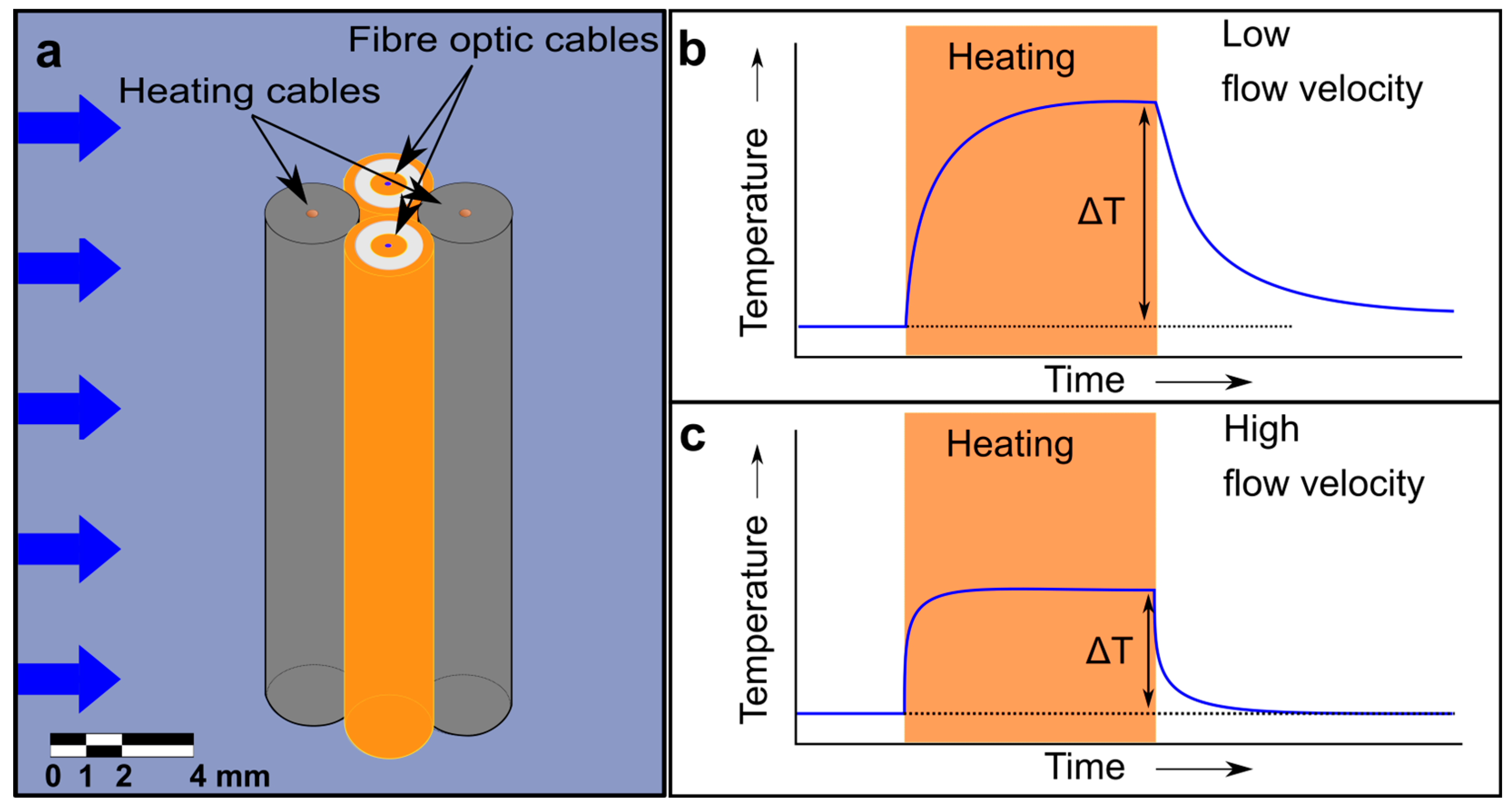
In active heating distributed temperature sensing (AH-DTS), a heating element is combined with measurements along a fiber-optic cable. If the heating element is at a significant distance (e.g., more than ~a few cm) from the fiber-optic cable, the experiment is considered to be a tracer experiment and not an AH-DTS setup. Figure 3a shows an example of a proper AH-DTS cable setup containing two heating wires and two fiber-optic cables. Heat is generated by applying electrical power to the heating wire. The electrical resistance of the cable will allow for an even heating of the cable over its length (electrical resistance heating). The AH-DTS cable is heated for a known duration, and the temperature is continuously measured. The difference in temperature between the background (initial) temperature and the maximum temperature during heating (ΔT) is directly related to the groundwater flow velocity (Figure 3b,c). ΔT will decrease by an increasing flow velocity due to the increasing advection of the heat by the moving groundwater. For low flow velocities, depending on the time of heating, an equilibrium heated temperature may not be reached during the time of the experiment. This can be solved by the extrapolation of the observed data through curve fitting [64].

Applications of an AH-DTS setup for groundwater flow can be found in Bakx et al. [64], des Tombe and Bakker [65], and Godinaud et al. [66].

3.2. Typical Field Measurement Setups

3.2.1. Geoelectrical Measurements

To suit the measurement location and the goal, the method, setup, and array of the geoelectrical measurement need to be selected accordingly. Electrodes can be placed at the ground surface or placed into boreholes to increase depth resolution. For applications near drinking water extraction wells, it is important to consider the presence of metal components in the subsurface, as metal can interfere with the geoelectrical measurements. Parts of the well could be constructed using metal, or there might be water transport pipes present. A clear line between the placed electrodes, free of any metal bodies, is needed for a successful result.

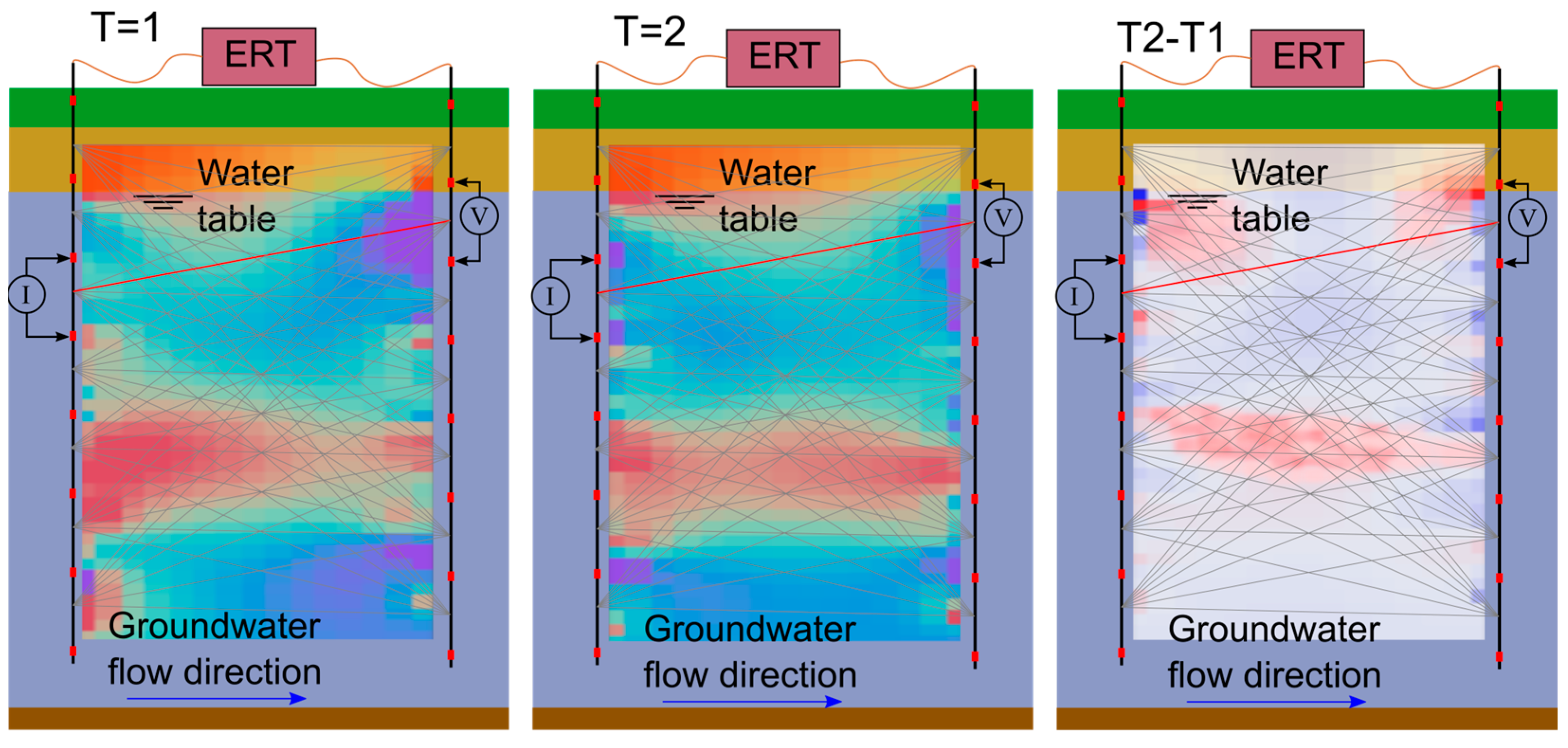
Using different setups, 2D + time or 3D + time (also considered as 4D) images of the subsurface can be achieved by increasing the number of electrodes used and extending/changing the setup of the electrodes. An example of a cross-borehole setup for 2D + time is shown in Figure 4. Using the electrodes placed in a cross-sectional line along the ground surface, or by using the electrodes from two boreholes (as shown in Figure 4), a cross-sectional resistivity image can be obtained after inversion. A 3D resistivity image is obtained by placing the electrodes in a grid across the ground surface, or by using multiple boreholes and measuring all the different combinations of electrodes. In 3D + time resistivity imaging, 3D imaging is conducted multiple times during a period of time with the same setup, thereby including the dimension time in the image, capturing the change in resistivity over time [57]. The dimension time can be included in the same way for 2D cross-sectional measurements (Figure 4, T1 and T2), resulting in a change in resistivity over time (Figure 4, T2-T1).

Different arrays of electrode setups are used. Dahlin and Zhou [67] defined the advantages and disadvantages of arrays for a basic setup of 10 electrodes for a 2D resistivity image by using numerical simulations. Currently, arrays can be optimized for specific situations and applications. The optimum array setup is related to the type of geoelectrical measurement. For cross-borehole measurement, different arrays are used, such as dipole–dipole, bipole–bipole, pole–tripole, and pole–dipole arrays. A more detailed explanation regarding cross-borehole ERT and array setup can be found in Loke et al. [68] and Zhou and Greenhalgh [69].

3.2.2. AH-DTS Measurements

A typical AH-DTS setup for measuring groundwater flow around drinking water extraction wells involves the use of AH-DTS cables vertically placed at different distances from the extraction well (Figure 5). Both a DTS, unit as well as a power supply, are placed at the ground surface and connected to the cables. Temperature is measured continuously by the DTS unit, and heat is applied for a fixed period. The difference ΔT between the background temperature and maximum temperature during heating is determined. The ΔT varies in relation to the change in velocity over depth and relative distance to the extraction well.

The installation of fiber-optic cables to measure natural groundwater flow is challenging, as direct contact with the aquifer sediments is needed. Placing fiber-optic cables in boreholes and refilling them with similar sediments is often the only solution. Clay sealings can be applied at the correct depths to prevent leaking through the filled borehole between separate aquifers. Good logging of sedimental layering during drilling is crucial for proper refilling, and during filling, additional time is required for the settling of the sediment. When sediment material and measurement depth allow, placement through the direct push technique (e.g., cone penetration), as suggested by Bakker et al. [30], can provide a solution. However, the direct push technique can create the smearing of sediment by the drive point, effecting the vertical sediment distribution directly around the placed cable.

3.3. Relating Geophysical Measurement to Groundwater Flow Velocities

3.3.1. Geoelectrical Measurements

Changes of resistivity over time measured using DCR or self-potential can be related to groundwater flow velocity, using temperature as an tracer. A time-lapse inversion of the geoelectrical data is needed, which adds the time dimension to the model discretization [70]. Algorithms for these inversions differ based on the geoelectrical measurement technique (DCR and SP), the measurement setup, and the arrays used. An overview and basic description of inverse modeling for DCR and SP is provided by Revil et al. [13]. For a basic understanding of solving the inverse problem, the reader is referred to Aster et al. [62].

When data is collected over sequential time-steps, (4D) ERT allows for the imaging of dynamic hydrogeologic effects such as changes in temperature (as a result of groundwater flow). There are several inversion strategies regarding how to handle the time component in the data and how to reduce the non-uniqueness (e.g., Hayley et al. [71]; Karaoulis et al. [72]; Kim et al. [73]; Loke et al. [68]), specifically, near extraction wells, a time-lapse ERT recording well on/well off and injection procedures results in changing electrical resistivity over time.

A change in electrical conductivity can be expected after a change in temperature as a result of the reduction in fluid viscosity and an increase in grain surface ionic mobility with an increasing temperature [74,75]. For temperatures up to 25 °C, an increase in the electrical conductivity by approximately 1.8–2.2% per °C is cited [74,76,77].

The change in the electrical tomograph resulting from the ERT can be physically interpreted by temperature by using a petrophysical transformation, as presented by Hermans et al. [75]:

$$T=\frac{{\sigma }_{b2}}{{\sigma }_{b1}}\left(T_1-T_{ref}\right)+\frac{\frac{{\sigma }_{b2}}{{\sigma }_{b1}}-1}{m_f{T}_{ref}}+T_{ref}$$

(1)

where $T$ is the temperature, ${\sigma }_{b1}$ and ${\sigma }_{b2}$ (S m⁻¹) are the measured bulk electrical conductivities, $T_1$ the initial temperature, $T_{ref}$ is the reference temperature, often taken as 25 °C, and $m_f{T}_{ref}$ (°C⁻¹) is the change in electrical conductivity per °C. However, alternative methods to interpret temperature from electrical conductivity can be found. Ma et al. [76] provide a comparison of several temperature correction models.

Several field applications show the use of 4D ERT, with heat as an geophysical tracer, as a successful method for understanding groundwater flow [78,79,80]. Additional relevant literature on the inverse modeling of geoelectrical measurements regarding groundwater flow velocity is provided in Appendix C,

Table A5. Literature on inverse modeling of geoelectrical measurements regarding groundwater flow velocity.

Measurement Technique	Setup	Model Result, Relevance	References
SP	2D, ground surface	The shape of the groundwater table in an unconfined aquifer	[63]
SP, temperature	2D, ground surface (SP), borehole (temp)	Joint inversion of temperature and self-potential algorithm estimating permeability	[147]
SP	2D, ground surface	Measuring streaming potential related to groundwater flow	[148]
DCR	4D time-lapse	ERT inversion allowing time and space to be part of the inverse modeling	[70,72]
SP	Laboratory	Modeling the spectral IP response to water-saturated sands	[149]
SP, hydraulic head pumping	2D/3D, ground surface, and point locations	Joint inversion of hydraulic head and self-potential data of harmonic pumping tests, hydraulic conductivity	[150]
DCR	2D, cross-borehole	Groundwater level, geological boundaries	[129]
DCR	3D, ground surface	3D joint inversion for seawater intrusion models	[151]

.

3.3.2. AH-DTS Measurements

The AH-DTS measurements can be translated into groundwater flow velocities by solving the heat flow equation, including both the conduction of the heat (through water, fiber-optic cable material, and sediment) and the convection by the movement of groundwater [11]:

$${\rho }_b{c}_b\frac{\partial T}{\partial t}=k_{eff}\left(\frac{{\partial }^{2}T}{\partial x^2}+\frac{{\partial }^{2}T}{\partial y^2}\right)-{\rho }_w{c}_w\left(q_x\frac{\partial T}{\partial x}+q_y\frac{\partial T}{\partial y}\right)+\frac{Q}{A}$$

(2)

In Equation (2) ${\rho }_b$ denotes the bulk density (kg mm⁻³) and $c_b$ the bulk specific heat capacity (J kg⁻¹ °C⁻¹) for the saturated sediment, and ${\rho }_w$ denotes the bulk density (kg m⁻³) and $c_w$ the bulk specific heat capacity for water. T denotes the temperature (°C), t is time (seconds), and $k_{eff}$ is the effective thermal conductivity of water and solids, (W m⁻¹ °C⁻¹). The components of the specific discharge vector are denoted by $q_x$ and $q_y$.

To solve the heat equation, the thermal properties of all mediums (e.g., water, fiber-optic cable materials, and sediment) need to be included. For a setup with the heating cable separated at a fixed distance from the fiber-optic cable, a solution for the heat equation providing groundwater flow velocities applied in an open borehole is given by Read et al. [81]. Bakx et al. [64] present a variation of this equation by calculating the groundwater flow velocity using an AH-DTS setup, with the heating cable directly attached to the fiber-optic cable placed in direct contact with the aquifer. Other variations are given by Bakker et al. [30], des Tombe and Bakker [65], and del Val et al. [82].

4. Discussion

4.1. Considerations for Measuring Groundwater Flow Velocities near Drinking Water Extraction Wells

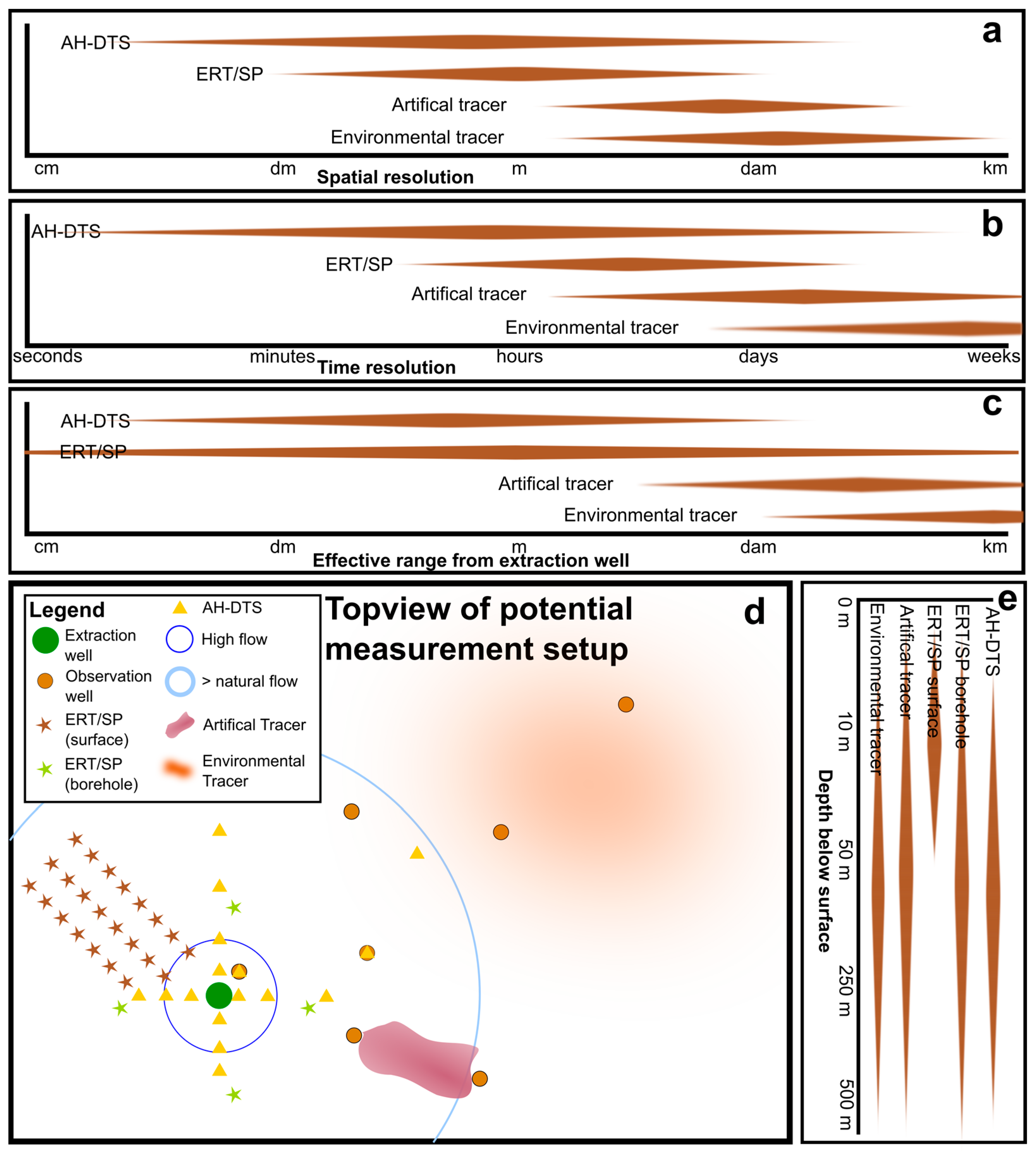
Opportunities for groundwater flow velocity measurement near drinking water extraction wells are limited due to restrictions for the protection of the water quality, but also due to the relative high flow velocities that are found close to the wells. In previous sections, we discussed the measurement techniques that are applicable near drinking water extraction wells which circumvent these restrictions. Figure 6 provides the main considerations for choosing and designing the best setup for measuring groundwater flow velocities near drinking water extraction wells.

When considering the distance to the extraction well, the use of artificial tracers is limited to larger distances from the well to protect the water quality. The required distance is related to the tracer used and the local legislation, but will normally be in the order of up to 1 km. Therefore, artificial tracer measurements are best used to estimate the regional flow around a well field using observation wells. If the use of artificial tracers is considered and allowed near drinking water extraction wells, for experiments within a 10 m radius of the well, high dilution rates should be expected due to the relatively high groundwater flow velocities making detecting of the tracer challenging. The spatial resolution and depth of application of artificial tracer measurements is directly related to the availability (or budget) and locations of the observation wells. Multi-well measurements can take hours up to days to complete, and traditional single-well measurements also can take hours to complete; however, newly developed techniques, such as the use of the In-Well Point Velocity Probe (IWPVP), can be considered for monitoring groundwater flow changes over time [26].

Environmental tracers can provide valuable insight into regional flow. Flow estimation is the most accurate when analyzing a stable situation so that aspects influencing the tracer can be identified. Near drinking water extraction wells, flow is more dynamic, making successful analyses challenging. Spatial resolution and the depth of the measurements are related to the availability of (or budget for) observations wells. Even though measurements (e.g., temperature using DTS) can be obtained in a short period of time (s), they can provide information on the average groundwater flow [12]. Due to the development of techniques for measuring temperature in a detailed and cost-efficient manner (e.g., DTS), temperature is the preferred choice over chemicals as a tracer.

Geoelectrical measurements are promising for mapping groundwater flow distributions (Figure 4). They can map groundwater flow near the extraction well in detail, or provide insight regarding the flow towards the extraction well on a larger scale. Meanwhile, different measurement setups which are also related to the well depth are needed. Detailed information can be obtained directly adjacent to the well by placing electrodes for measuring groundwater flow in boreholes at the depth of the well screen. Mapping the flow from ground surface levels provides a broader perspective around the well, but the depth of investigation is limited to at most 40 to 50 m, due to the decreasing resolution. The spatial resolution of the geoelectrical measurements is related to the relative distance between the electrodes. The typical resolutions used are in the range of 0.1 to 5 m. When the electrodes are placed at ground surface level, the resolution will decrease with depth. With increasing depth, a longer array of electrodes is needed. Setting up a geoelectrical mapping of a larger area can be time consuming. Time resolution is dependent on the number of electrodes placed in the grid, and it can take several minutes (single array) up to over an hour ( large setup) to measure the potential between all electrodes. For dedicated setups (e.g., setups placed in boreholes), automation can be used to collect measurements at set time intervals. Using time-lapse measurements, changes in resistivity can also be mapped and related to groundwater flow. While measurements at ground surface level can be executed at relative low cost (setup and electrodes can also be used for other project afterwards), installing a dedicated system in boreholes is costly, as the placed electrodes cannot be reused for other projects.

AH-DTS measurements can provide direct measurements of groundwater flow velocities near drinking water extraction wells, specifically in the high flow area within 10 m of the well (Figure 5). The spatial resolution of a measurement setup is related to the number of cables placed and the relative distance between the cables. Along the fiber-optic cable, sampling intervals of up to 12.9 cm are possible when using DTS. Smaller intervals can be reached when using FBG or R-DTS. Time resolution depends on the required/optimum heating time of the cable, which in recent setups, was set to approximately 1 to 2 h [65]. Further research on the interpretation of AH-DTS is needed to reduce the heating time, i.e., by relating the steepness of the heating curve to the groundwater flow velocity. The accuracy of AH-DTS makes its application for detecting temporal changes in more natural low groundwater flow velocities challenging. The costly installation of AH-DTS cables directly into the subsurface should be considered with care. Further development of the technique for accurate measurements placed within observation wells will increase the potential for measuring regional groundwater flow. Although placement costs (e.g., drilling costs) can be high for installing AH-DTS, the fiber-optic cables themselves are relatively inexpensive. When higher resolutions with FBG or DTS-R are considered, one should budget the relatively higher costs of these cables, as they must be designed and constructed specifically for the experiment.

In addition to measuring groundwater flow velocity directly, insights and developments in measuring and understanding hydraulic properties of sediments further improves the understanding of groundwater flow in drinking water extraction well fields. An example is the research and modeling regarding groundwater flow in faulted rock masses [83].

4.2. Potential for Measuring Groundwater Flow near Drinking Water Extraction Wells

The combination of measurement techniques is instrumental in estimating fine-scale groundwater flow velocities around drinking water extraction wells. Other groundwater measurement related studies show this potential. For instance, a combination of DCR, induced polarization, and fiber-optic DTS has already been applied to study the groundwater–surface water interaction [84]. Geoelectrical data were used to estimate lithological variations, while DTS data was used to locate the exchange of groundwater and surface water at a 1 m resolution and 5 min sampling. Hermans et al. [80] compared the potential for temperature monitoring of DTS and cross-borehole ERT, showing an error between 10–20% using the ERT, and determined a threshold of 1.2 °C. However, to our knowledge, there is no combination of these geophysical methods to estimate groundwater flow velocities. In

Table 1. Case studies using the ERT, SP, or AH-DTS technique for temperature tracing in groundwater or measuring groundwater flow directly, providing some successful examples and showing the spatial/temporal resolution, accuracy, and the range of the measured groundwater flow velocities for these studies.

Technique	Parameter	Spatial Resolution	Temporal Resolution	Accuracy/Range of Measurements	Reference
ERT	Temperature tracing	0.25 m × 0.25 m (inversion)	45 min	10–20% error and 1.2 °C threshold	Hermans et al. [80]
	Temperature tracing	3 m	35 to 120 min	Resistivity variations >1%	Robert et al. [78]
	Groundwater flow velocity *	0.05 m (experiment setup)	N/A	5% velocity/2.5–11.6 m/day	Chen et al. [53]
SP	Groundwater flow velocity	1 m	N/A	Not specified/0.4–0.47 m/day	Jardani et al. [60]
	Groundwater flow velocity	1.5 m	N/A	Not specified/0.25–2.5 m/day	Ikard et al. [85]
	Groundwater flow velocity	Not mentioned	N/A	RMSE 1.2%/0.02–0.12 m/d	Richards et al. [56]
AH-DTS	Water flow in borehole	0.29 m	5 min	Not specified/0–0.6 m/day	Read et al. [81]
	Groundwater flow **	2 m	1 day	Not specified/relative flow	Selker and selker [86]
	Groundwater flow velocity *	1 m	1.5 h	R2 is 0.85/0–9 m/day	Bakx et al. [64]

* Experimental setup was used on these case studies (on a laboratory scale); ** case study in a 600 m borehole determining variation of groundwater flow over depth.

, a selection of case studies showing the potential of the measurement techniques to estimate temperature and groundwater flow velocity is provided.

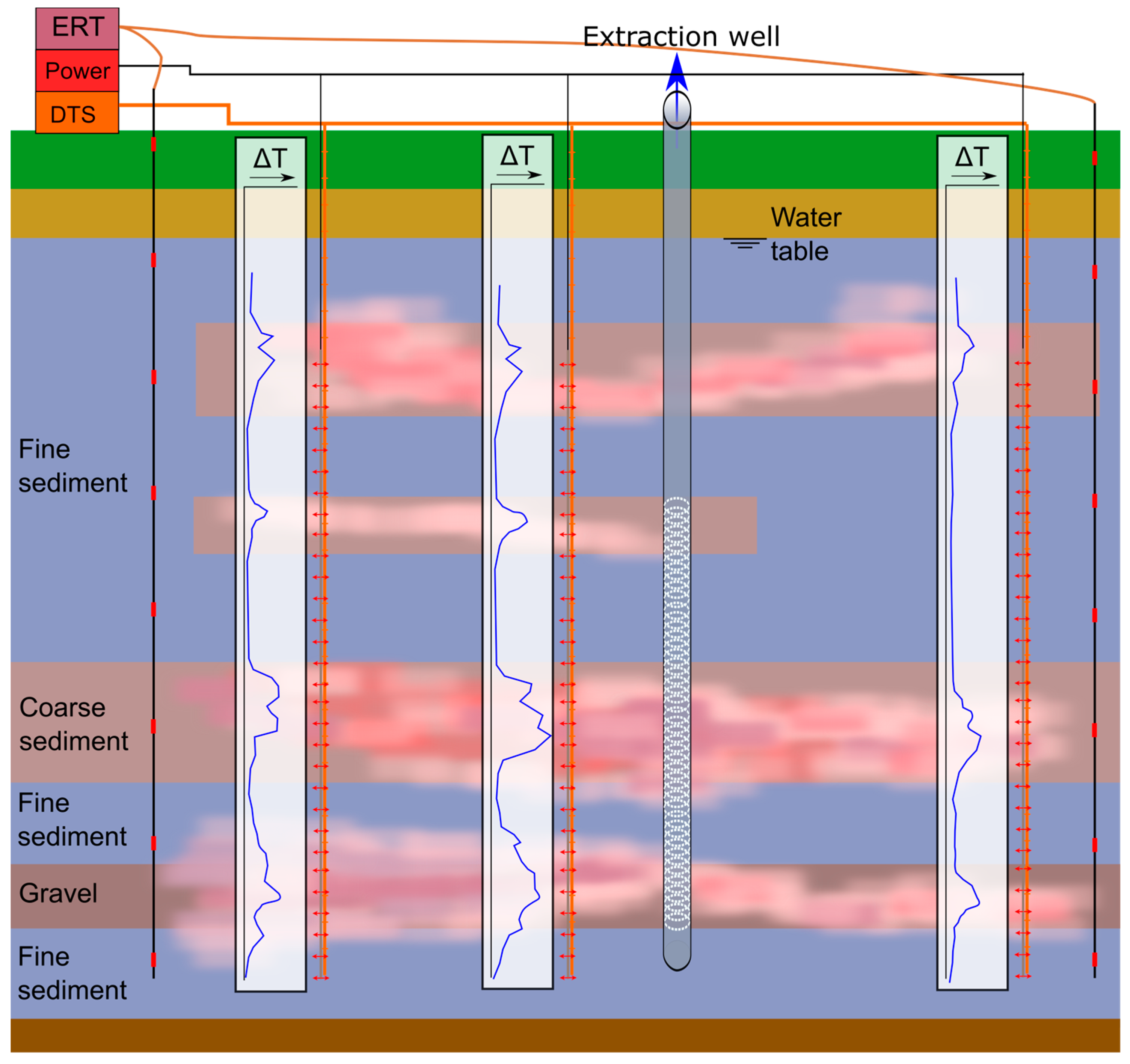
This potential is shown conceptually in Figure 7, proposing how AH-DTS would combine with DCR time-lapse measurements. Time-lapse DCR measurements are used to highlight areas of large changes in resistivity as an indication of preferential groundwater flow paths. The AH-DTS measurements within this measured field provide groundwater flow velocities at several locations and over the depth, if cables are placed vertically. Both results can be combined to arrive at 3D estimates of the groundwater flow velocities around the extraction well. As an alternative to DCR time-lapse measurements, SP measurements, also capable of showing preferential flow, can be used in combination with AH-DTS. The application of these combined measurement setups as monitoring systems holds the potential to measure small-scale changes in groundwater flow velocities over time, for instance, in response to groundwater depletion or well clogging, which may be used to guide interventions to avoid these occurrences.

5. Conclusions

We reviewed techniques suitable for measuring groundwater flow velocities in unconsolidated sediments near drinking water extraction wells. We evaluated tracer-based methods, geoelectrical methods (ERT and SP), and active heating-distributed temperature sensing (AH-DTS).

The use of tracer measurements is a reliable method to estimate groundwater flow velocities at the regional scale. However, its use close to drinking water extraction wells is more limited due to imposed restrictions around drinking water facilities and the high dilution rates that result from the high flow velocities around wells. Temperature is a reliable tracer that holds no direct risk for impacting water quality.

Geoelectrical measurements (e.g., ERT or SP) can be used to estimate and map variations in subsurface structures, hydraulic conductivity, and preferential flow paths. Time-lapse measurements can show changes in groundwater flow when a tracer (e.g., temperature) that provides a contrast in electrical resistivity is used, which can then be used to estimate flow velocities. If electrodes/receivers are placed at the surface only, the resolution of the measurements decreases with depth. Cross-borehole measurements using multiple electrodes and receivers with depth can also provide high-resolution results at greater depths. Geoelectrical measurements can be used near drinking water extraction wells, but the influence of metal present within the well or supply pipelines must be considered.

Active heating-distributed temperature sensing (AH-DTS) measurements can be used to estimate groundwater flow velocity over long stretches of cable at high spatial resolution. Using fiber Bragg grating and DTS-R (Rayleigh-based DTS) instead of DTS, in combination with an active heating element, make it possible to perform groundwater flow velocity measurements, even up to mm scale resolution. These types of measurements are suitable for laboratory environments, where they can be used to provide new insights into the effect of small-scale heterogeneity on groundwater flow. For field applications, an AH-DTS is more cost efficient than FBG or DTS-R. For measuring the relative high flow velocities directly adjacent to the drinking water extraction well, AH-DTS is the most promising method.

Combining geophysical measurement techniques can provide additional insight into groundwater flow around drinking water extraction wells. A measurement setup is presented in which time-lapse ERT is used to map detailed groundwater flow patterns in the subsurface around the extraction well. AH-DTS measurements near the extraction well provide detailed groundwater flow velocity data. A 3D groundwater flow velocity image can potentially be obtained by interpolation of the combined data.

References

- Wada, Y.; Van Beek, L.P.H.; Van Kempen, C.M.; Reckman, J.W.T.M.; Vasak, S.; Bierkens, M.F.P. Global Depletion of Groundwater Resources. Geophys. Res. Lett. 2010, 37, 1–5. [Google Scholar] [CrossRef] [Green Version]
- Fleuchaus, P.; Godschalk, B.; Stober, I.; Blum, P. Worldwide Application of Aquifer Thermal Energy Storage—A Review. Renew. Sustain. Energy Rev. 2018, 94, 861–876. [Google Scholar] [CrossRef]
- Famiglietti, J.S. The Global Groundwater Crisis. Nat. Clim. Change 2014, 4, 945–948. [Google Scholar] [CrossRef] [Green Version]
- Leaf, A.T.; Hart, D.J.; Bahr, J.M. Active Thermal Tracer Tests for Improved Hydrostratigraphic Characterization. Ground Water 2012, 50, 726–735. [Google Scholar] [CrossRef] [PubMed]
- Bayer, P.; Huggenberger, P.; Renard, P.; Comunian, A. Three-Dimensional High Resolution Fluvio-Glacial Aquifer Analog: Part 1: Field Study. J. Hydrol. 2011, 405, 1–9. [Google Scholar] [CrossRef] [Green Version]
- Kaufman, W.J.; Orlob, G.T. An Evaluation of Ground-Water Tracers. Trans. Am. Geophys. Union 1956, 87, 297–306. [Google Scholar] [CrossRef]
- Evans, G.V. Tracer Techniques in Hydrology. Int. J. Appl. Radiat. Isot. 1983, 34, 451–475. [Google Scholar] [CrossRef]
- Bethke, C.M.; Johnson, T.M. Groundwater Age and Groundwater Age Dating. Annu. Rev. Earth Planet. Sci. 2007, 36, 121–152. [Google Scholar] [CrossRef] [Green Version]
- Chambers, L.A.; Gooddy, D.C.; Binley, A.M. Use and Application of CFC-11, CFC-12, CFC-113 and SF6 as Environmental Tracers of Groundwater Residence Time: A Review. Geosci. Front. 2018, 10, 1643–1652. [Google Scholar] [CrossRef]
- Cartwright, I.; Cendón, D.; Currell, M.; Meredith, K. A Review of Radioactive Isotopes and Other Residence Time Tracers in Understanding Groundwater Recharge: Possibilities, Challenges, and Limitations. J. Hydrol. 2017, 555, 797–811. [Google Scholar] [CrossRef]
- Anderson, M.P. Heat as a Ground Water Tracer. Groundwater 2005, 43, 951–968. [Google Scholar] [CrossRef] [PubMed]
- Kurylyk, B.L.; Irvine, D.J.; Bense, V.F. Theory, Tools, and Multidisciplinary Applications for Tracing Groundwater Fluxes from Temperature Profiles. Wiley Interdiscip. Rev. Water 2019, 6, e1329. [Google Scholar] [CrossRef] [Green Version]
- Revil, A.; Karaoulis, M.; Johnson, T.; Kemna, A. Review: Some Low-Frequency Electrical Methods for Subsurface Characterization and Monitoring in Hydrogeology. Hydrogeol. J. 2012, 20, 617–658. [Google Scholar] [CrossRef]
- Bense, V.F.; Read, T.; Le Borgne, T.; Coleman, T.I.; Krause, S.; Chalari, A.; Mondanos, M.J.; Ciocca, F.; Selker, J.S. Distributed Temperature Sensing as a Downhole Tool in Hydrogeology. Water Resour. Res. 2016, 52, 9259–9273. [Google Scholar] [CrossRef] [Green Version]
- Hatfield, K.; Annable, M.; Cho, J.; Rao, P.S.C.; Klammler, H. A Direct Passive Method for Measuring Water and Contaminant Fluxes in Porous Media. J. Contam. Hydrol. 2004, 75, 155–181. [Google Scholar] [CrossRef]
- Freeze, R.A.; Cherry, J.A. Groundwater; Prentice-Hall Inc.: Englewood Cliffs, NJ, USA, 1979; ISBN 0-13-365312-9. [Google Scholar]
- Barth, G.R.; Illangasekare, T.H.; Hill, M.C.; Rajaram, H. A New Tracer-Density Criterion for Heterogeneous Porous Media. Water Resour. Res. 2001, 37, 21–31. [Google Scholar] [CrossRef] [Green Version]
- Ma, R.; Zheng, C. Effects of Density and Viscosity in Modeling Heat as a Groundwater Tracer. Ground Water 2010, 48, 380–389. [Google Scholar] [CrossRef]
- Driscoll, F.G. Groundwater and Wells, 2nd ed.; Johnson Screens: St. Paul, MN, USA, 1986; ISBN 0-9616456-0-1. [Google Scholar]
- Drost, W.; Klotz, D.; Koch, A.; Moser, H.; Neumaier, F.; Rauert, W. Point Dilution Methods of Investigating Ground Water Flow by Means of Radioisotopes. Water Resour. Res. 1968, 4, 125–146. [Google Scholar] [CrossRef]
- Maldaner, C.H.; Munn, J.D.; Coleman, T.I.; Molson, J.W.; Parker, B.L. Groundwater Flow Quantification in Fractured Rock Boreholes Using Active Distributed Temperature Sensing Under Natural Gradient Conditions. Water Resour. Res. 2019, 55, 3285–3306. [Google Scholar] [CrossRef]
- Pitrak, M.; Mares, S.; Kobr, M. A Simple Borehole Dilution Technique in Measuring Horizontal Ground Water Flow. Ground Water 2007, 45, 89–92. [Google Scholar] [CrossRef]
- Kaplan, P.; Leap, D. A Single-Well, Multiple-Pulse Tracer Technique for Estimating Ground Water Velocities and Pollutant Transport Rates: Phase I—Theoretical Development; Purdue University: West Lafayette, IN, USA, 1984. [Google Scholar]
- Jamin, P.; Brouyère, S. Monitoring Transient Groundwater Fluxes Using the Finite Volume Point Dilution Method. J. Contam. Hydrol. 2018, 218, 10–18. [Google Scholar] [CrossRef]
- Annable, M.D.; Hatfield, K.; Cho, J.; Klammler, H.; Parker, B.L.; Cherry, J.A.; Rao, P.S.C. Field-Scale Evaluation of the Passive Flux Meter for Simultaneous Measurement of Groundwater and Contaminant Fluxes. Environ. Sci. Technol. 2005, 39, 7194–7201. [Google Scholar] [CrossRef]
- Osorno, T.C.; Devlin, J.F.; Firdous, R. An In-Well Point Velocity Probe for the Rapid Determination of Groundwater Velocity at the Centimeter-Scale. J. Hydrol. 2018, 557, 539–546. [Google Scholar] [CrossRef]
- Flury, M.; Wai, N.N. Dyes as Tracers for Vadose Zone Hydrology. Rev. Geophys. 2003, 41, 1002. [Google Scholar] [CrossRef]
- Read, T.; Bense, V.F.; Bour, O.; Le Borgne, T.; Lavenant, N.; Hochreutener, R.; Selker, J.S. Thermal-Plume Fibre Optic Tracking (T-POT) Test for Flow Velocity Measurement in Groundwater Boreholes. Geosci. Instrum. Methods Data Syst. Discuss. 2015, 5, 161–175. [Google Scholar] [CrossRef] [Green Version]
- Liu, G.; Knobbe, S.; Butler, J.J. Resolving Centimeter-Scale Flows in Aquifers and Their Hydrostratigraphic Controls. Geophys. Res. Lett. 2013, 40, 1098–1103. [Google Scholar] [CrossRef]
- Bakker, M.; Calje, R.; Schaars, F.; van der Made, K.-J.; de Haas, S. An Active Heat Tracer Experiment to Determine Groundwater Velocities Using Fiber Optic Cables Installed with Direct Push Equipment. J. Hydrol. 2015, 51, 2760–2772. [Google Scholar] [CrossRef] [Green Version]
- Read, T.; Bour, O.; Bense, V.; Le Borgne, T.; Goderniaux, P.; Klepikova, M.V.; Hochreutener, R.; Lavenant, N.; Boschero, V. Characterizing Groundwater Flow and Heat Transport in Fractured Rock Using Fiber-Optic Distributed Temperature Sensing. Geophys. Res. Lett. 2013, 40, 2055–2059. [Google Scholar] [CrossRef] [Green Version]
- Selker, J.S.; Thévenaz, L.; Huwald, H.; Mallet, A.; Luxemburg, W.; Van De Giesen, N.; Stejskal, M.; Zeman, J.; Westhoff, M.; Parlange, M.B. Distributed Fiber-Optic Temperature Sensing for Hydrologic Systems. Water Resour. Res. 2006, 42, 1–8. [Google Scholar] [CrossRef] [Green Version]
- Sang, A.K.; Froggatt, M.E.; Gifford, D.K.; Kreger, S.T.; Dickerson, B.D. One Centimeter Spatial Resolution Temperature Measurements in a Nuclear Reactor Using Rayleigh Scatter in Optical Fiber. IEEE Sens. J. 2008, 8, 1375–1380. [Google Scholar] [CrossRef]
- Alemohammad, H.; Azhari, A.; Liang, R. Fiber Optic Sensors for Distributed Monitoring of Soil and Groundwater during In-Situ Thermal Remediation. Fiber Opt. Sens. Appl. XIV 2017, 10208, 102080I. [Google Scholar] [CrossRef]
- van de Giesen, N.; Steele-Dunne, S.C.; Jansen, J.; Hoes, O.; Hausner, M.B.; Tyler, S.; Selker, J. Double-Ended Calibration of Fiber-Optic Raman Spectra Distributed Temperature Sensing Data. Sensors 2012, 12, 5471–5485. [Google Scholar] [CrossRef] [Green Version]
- Hausner, M.B.; Suárez, F.; Glander, K.E.; van de Giesen, N.; Selker, J.S.; Tyler, S.W. Calibrating Single-Ended Fiber-Optic Raman Spectra Distributed Temperature Sensing Data. Sensors 2011, 11, 10859–10879. [Google Scholar] [CrossRef]
- Tyler, S.W.; Selker, J.S.; Hausner, M.B.; Hatch, C.E.; Torgersen, T.; Thodal, C.E.; Schladow, S.G. Environmental Temperature Sensing Using Raman Spectra DTS Fiber-Optic Methods. Water Resour. Res. 2009, 45, 1–11. [Google Scholar] [CrossRef] [Green Version]
- Baldini, F.; Brenci, M.; Chiavaioli, F.; Giannetti, A.; Trono, C. Optical Fibre Gratings as Tools for Chemical and Biochemical Sensing. Anal. Bioanal. Chem. 2012, 402, 109–116. [Google Scholar] [CrossRef]
- Jasechko, S. Partitioning Young and Old Groundwater with Geochemical Tracers. Chem. Geol. 2016, 427, 35–42. [Google Scholar] [CrossRef]
- Priestley, S.C.; Wohling, D.L.; Keppel, M.N.; Post, V.E.A.; Love, A.J.; Shand, P.; Tyroller, L.; Kipfer, R. Detecting Inter-Aquifer Leakage in Areas with Limited Data Using Hydraulics and Multiple Environmental Tracers, Including 4He, 36Cl/Cl, 14C and 87Sr/86Sr. Hydrogeol. J. 2017, 25, 2031–2047. [Google Scholar] [CrossRef] [Green Version]
- Post, V.E.A.; Houben, G.J.; Stoeckl, L.; Sültenfuß, J. Behaviour of Tritium and Tritiogenic Helium in Freshwater Lens Groundwater Systems: Insights from Langeoog Island, Germany. Geofluids 2019, 2019, 1494326. [Google Scholar] [CrossRef] [Green Version]
- Stallman, R.W. Steady One-Dimensional Fluid Flow in a Semi-Infinite Porous Medium with Sinusoidal Surface Temperature. J. Geophys. Res. 1965, 70, 2821–2827. [Google Scholar] [CrossRef]
- Saar, M.O. Review: Geothermal Heat as a Tracer of Large-Scale Groundwater Flow and as a Means to Determine Permeability Fields. Hydrogeol. J. 2011, 19, 31–52. [Google Scholar] [CrossRef]
- Bredehoeft, J.D.; Papaopulos, I.S. Rates of Vertical Groundwater Movement Estimated from the Earth’s Thermal Profile. Water Resour. Res. 1965, 1, 325–328. [Google Scholar] [CrossRef]
- Kurylyk, B.L.; Irvine, D.J.; Carey, S.K.; Briggs, M.A.; Werkema, D.D.; Bonham, M. Heat as a Groundwater Tracer in Shallow and Deep Heterogeneous Media: Analytical Solution, Spreadsheet Tool, and Field Applications. Hydrol. Process. 2017, 31, 2648–2661. [Google Scholar] [CrossRef] [PubMed]
- Taniguchi, M.; Williamson, D.R.; Peck, A.J. Disturbances of Temperature-Depth Profiles Due to Surface Climate Change and Subsurface Water Flow: 2. An Effect of Step Increase in Surface Temperature Caused by Forest Clearing in Southwest Western Australia. Water Resour. Res. 1999, 35, 1519–1529. [Google Scholar] [CrossRef]
- Kurylyk, B.L.; Macquarrie, K.T.B. A New Analytical Solution for Assessing Climate Change Impacts on Subsurface Temperature. Hydrol. Process. 2014, 28, 3161–3172. [Google Scholar] [CrossRef]
- Kurylyk, B.L.; Irvine, D.J. Analytical Solution and Computer Program (FAST) to Estimate Fluid Fluxes from Subsurface Temperature Profiles. Water Resour. Res. 2016, 52, 725–733. [Google Scholar] [CrossRef] [Green Version]
- Bense, V.F.; Kurylyk, B.L.; van Daal, J.; van der Ploeg, M.J.; Carey, S.K. Interpreting Repeated Temperature-Depth Profiles for Groundwater Flow. Water Resour. Res. 2017, 53, 8639–8647. [Google Scholar] [CrossRef]
- Binley, A.; Slater, L.D.; Fukes, M.; Cassiani, G. Relationship between Spectral Induced Polarization and Hydraulic Properties of Saturated and Unsaturated Sandstone. Water Resour. Res. 2005, 41, 1–13. [Google Scholar] [CrossRef]
- Rubin, Y.; Hubbard, S.S. Hydrogeophysics; Springer: Amsterdam, The Netherlands, 2005; ISBN 9781402031014. [Google Scholar]
- Revil, A.; Titov, K.; Doussan, C.; Lapenna, V. Applications of the Self-Potential Method to Hydrological Problems. In Applied Hydrogeophysics; Springer: Amsterdam, The Netherlands, 2006; pp. 255–292. [Google Scholar]
- Chen, J.L.; Chen, C.H.; Kuo, C.L.; Fen, C.S.; Wu, C.C. Estimating Groundwater Velocity Using Apparent Resistivity Tomography: A Sandbox Experiment. IOP Conf. Ser. Earth Environ. Sci. 2016, 39, 012056. [Google Scholar] [CrossRef]
- Dahlin, T. The Development of DC Resistivity Imaging Techniques. Comput. Geosci. 2001, 27, 1019–1029. [Google Scholar] [CrossRef] [Green Version]
- Seidel, K.; Lange, G. Direct Current Resistivity Methods. In Environmental Geology; Springer: Berlin/Heidelberg, Germany, 2007; pp. 205–237. [Google Scholar] [CrossRef]
- Richards, K.; Revil, A.; Jardani, A.; Henderson, F.; Batzle, M.; Haas, A. Pattern of Shallow Ground Water Flow at Mount Princeton Hot Springs, Colorado, Using Geoelectrical Methods. J. Volcanol. Geotherm. Res. 2010, 198, 217–232. [Google Scholar] [CrossRef]
- Loke, M.H.; Chambers, J.E.; Rucker, D.F.; Kuras, O.; Wilkinson, P.B. Recent Developments in the Direct-Current Geoelectrical Imaging Method. J. Appl. Geophys. 2013, 95, 135–156. [Google Scholar] [CrossRef]
- Binley, A.; Cassiani, G.; Middleton, R.; Winship, P. Vadose Zone Flow Model Parameterisation Using Cross-Borehole Radar and Resistivity Imaging. J. Hydrol. 2002, 267, 147–159. [Google Scholar] [CrossRef]
- Hayashi, M. Temperature-electrical conductivity relation of water for environmental monitoring and geophysical data inversion. Environ. Monit. Assess. 2004, 96, 119–128. [Google Scholar] [CrossRef] [PubMed]
- Jardani, A.; Revil, A.; Boleve, A.; Crespy, A.; Dupont, J.P.; Barrash, W.; Malama, B. Tomography of the Darcy Velocity from Self-Potential Measurements. Geophys. Res. Lett. 2007, 34, 1–6. [Google Scholar] [CrossRef] [Green Version]
- Slater, L.D.; Lesmes, D. The Induced Polarization Method. In Proceedings of the First International Conference on the Application of Geophysical Methodologies and NDT to Transportation Facilities and Infrastructure, St. Louis, MO, USA, December 2000; pp. 1–8. [Google Scholar]
- Aster, R.C.; Borchers, B.; Thurber, C. Parameter Estimation and Inverse Problems; Elsevier: Amsterdam, The Netherlands, 2005; Volume 2, ISBN 0-12-065604-3. [Google Scholar]
- Jardani, A.; Revil, A.; Akoa, F.; Schmutz, M.; Florsch, N.; Dupont, J.P. Least Squares Inversion of Self-Potential (SP) Data and Application to the Shallow Flow of Ground Water in Sinkholes. Geophys. Res. Lett. 2006, 33, 1–5. [Google Scholar] [CrossRef] [Green Version]
- Bakx, W.; Doornenbal, P.; van Weesep, R.; Bense, V.F.; Oude Essink, G.H.P.; Bierkens, M.F.P. Determining the Relation between Groundwater Flow Velocities and Measured Temperature Differences Using Active Heating-Distributed Temperature Sensing. Water 2019, 11, 1619. [Google Scholar] [CrossRef] [Green Version]
- Des Tombe, B.F.; Bakker, M. Estimation of the Variation in Specific Discharge Over Large Depth Using Distributed Temperature Sensing (DTS) Measurements of the Heat Pulse Response. Water Resour. Res. 2019, 55, 811–826. [Google Scholar] [CrossRef] [Green Version]
- Godinaud, J.; Klepikova, M.; Larroque, F.; Guihéneuf, N.; Dupuy, A.; Bour, O. Clogging Detection and Productive Layers Identification along Boreholes Using Active Distributed Temperature Sensing. J. Hydrol. 2023, 617, 554–568. [Google Scholar] [CrossRef]
- Dahlin, T.; Zhou, B. A Numerical Comparison of 2D Resistivity Imaging with 10 Electrode Arrays. Geophys. Prospect. 2004, 52, 379–398. [Google Scholar] [CrossRef] [Green Version]
- Loke, M.H.; Wilkinson, P.B.; Chambers, J.E.; Strutt, M. Optimized Arrays for 2D Cross-Borehole Electrical Tomography Surveys. Geophys. Prospect. 2014, 62, 172–189. [Google Scholar] [CrossRef] [Green Version]
- Zhou, B.; Greenhalgh, S.A. Cross-Hole Resistivity Tomography Using Different Electrode Configurations. Geophys. Prospect. 2000, 48, 887–912. [Google Scholar] [CrossRef]
- Karaoulis, M.; Tsourlos, P.; Kim, J.H.; Revill, a. 4D Time-Lapse ERT Inversion: Introducing Combined Time and Space Constraints. Near Surf. Geophys. 2014, 12, 25–34. [Google Scholar] [CrossRef] [Green Version]
- Hayley, K.; Pidlisecky, A.; Bentley, L.R. Simultaneous Time-Lapse Electrical Resistivity Inversion. J. Appl. Geophys. 2011, 75, 401–411. [Google Scholar] [CrossRef]
- Karaoulis, M.; Revil, a.; Werkema, D.D.; Minsley, B.J.; Woodruff, W.F.; Kemna, a. Time-Lapse Three-Dimensional Inversion of Complex Conductivity Data Using an Active Time Constrained (ATC) Approach. Geophys. J. Int. 2011, 187, 237–251. [Google Scholar] [CrossRef] [Green Version]
- Kim, J.-H.; Yi, M.-J.; Park, S.; Kim, J.-G. 4-D Inversion of DC Resistivity Monitoring Data Acquired over a Dynamically Changing Earth Model. J. Appl. Geophys. 2009, 68, 522–532. [Google Scholar] [CrossRef]
- Hayley, K.; Bentley, L.R.; Gharibi, M.; Nightingale, M. Low Temperature Dependence of Electrical Resistivity: Implications for near Surface Geophysical Monitoring. Geophys. Res. Lett. 2007, 34, L18402. [Google Scholar] [CrossRef]
- Hermans, T.; Nguyen, F.; Robert, T.; Revil, A. Geophysical Methods for Monitoring Temperature Changes in Shallow Low Enthalpy Geothermal Systems. Energies 2014, 7, 5083–5118. [Google Scholar] [CrossRef] [Green Version]
- Ma, R.; McBratney, A.; Whelan, B.; Minasny, B.; Short, M. Comparing Temperature Correction Models for Soil Electrical Conductivity Measurement. Precis. Agric. 2011, 12, 55–66. [Google Scholar] [CrossRef]
- Corwin, D.L.; Lesch, S.M. Apparent Soil Electrical Conductivity Measurements in Agriculture. Comput. Electron. Agric. 2005, 46, 11–43. [Google Scholar] [CrossRef]
- Robert, T.; Paulus, C.; Bolly, P.Y.; Lin, E.K.S.; Hermans, T. Heat as a Proxy to Image Dynamic Processes with 4D Electrical Resistivity Tomography. Geosciences 2019, 9, 414. [Google Scholar] [CrossRef] [Green Version]
- Hermans, T.; Vandenbohede, A.; Lebbe, L.; Nguyen, F. A Shallow Geothermal Experiment in a Sandy Aquifer Monitored Using Electric Resistivity Tomography. Geophysics 2012, 77, B11–B21. [Google Scholar] [CrossRef] [Green Version]
- Hermans, T.; Wildemeersch, S.; Jamin, P.; Orban, P.; Brouyère, S.; Dassargues, A.; Nguyen, F. Quantitative Temperature Monitoring of a Heat Tracing Experiment Using Cross-Borehole ERT. Geothermics 2015, 53, 14–26. [Google Scholar] [CrossRef] [Green Version]
- Read, T.; Bour, O.; Selker, J.S.; Bense, V.F.; Le Borgne, T.; Hochreutener, R.; Lavenant, N. Active-Distributed Temperature Sensing to Continuously Quantify Vertical Flow in Boreholes. Water Resour. Res. 2014, 50, 3706–3713. [Google Scholar] [CrossRef] [Green Version]
- del Val, L.; Carrera, J.; Pool, M.; Martínez, L.; Casanovas, C.; Bour, O.; Folch, A. Heat Dissipation Test with Fiber-Optic Distributed Temperature Sensing to Estimate Groundwater Flux. Water Resour. Res. 2021, 57, e2020WR027228. [Google Scholar] [CrossRef]
- Ma, D.; Duan, H.; Zhang, J.; Liu, X.; Li, Z. Numerical Simulation of Water–Silt Inrush Hazard of Fault Rock: A Three-Phase Flow Model. Rock Mech. Rock Eng. 2022, 55, 5163–5182. [Google Scholar] [CrossRef]
- Slater, L.D.; Ntarlagiannis, D.; Day-Lewis, F.D.; Mwakanyamale, K.; Versteeg, R.J.; Ward, A.; Strickland, C.; Johnson, C.D.; Lane, J.W. Use of Electrical Imaging and Distributed Temperature Sensing Methods to Characterize Surface Water-Groundwater Exchange Regulating Uranium Transport at the Hanford 300 Area, Washington. Water Resour. Res. 2010, 46, W10533. [Google Scholar] [CrossRef]
- Ikard, S.J.; Revil, A.; Schmutz, M.; Karaoulis, M.; Jardani, A.; Mooney, M. Characterization of Focused Seepage through an Earthfill Dam Using Geoelectrical Methods. Groundwater 2014, 52, 952–965. [Google Scholar] [CrossRef] [PubMed]
- Selker, F.; Selker, J.S. Investigating Water Movement within and near Wells Using Active Point Heating and Fiber Optic Distributed Temperature Sensing. Sensors 2018, 18, 1023. [Google Scholar] [CrossRef] [Green Version]
- Piccinini, L.; Fabbri, P.; Pola, M. Point Dilution Tests to Calculate Groundwater Velocity: An Example in a Porous Aquifer in Northeast Italy. Hydrol. Sci. J. 2016, 61, 1512–1523. [Google Scholar] [CrossRef] [Green Version]
- Mahler, N.; Sale, T.; Smith, T.; Lyverse, M. Use of Single-Well Tracer Dilution Tests to Evaluate LNAPL Flux at Seven Field Sites. Ground Water 2012, 50, 851–860. [Google Scholar] [CrossRef]
- Gouze, P.; Le Borgne, T.; Leprovost, R.; Lods, G.; Poidras, T.; Pezard, P. Non-Fickian Dispersion in Porous Media: 1. Multiscale Measurements Using Single-Well Injection Withdrawal Tracer Tests. Water Resour. Res. 2008, 44, 1–15. [Google Scholar] [CrossRef] [Green Version]
- Molz, F.J.; Guven, O.; Melville, J.G.; Crocker, R.D.; Matteson, K.T. Performance, Analysis, and Simulation of a 2-Well Tracer Test at the Mobile Site. Water Resour. Res. 1986, 22, 1031–1037. [Google Scholar] [CrossRef]
- Sutton, D.J.; Kabala, Z.J.; Schaad, D.E.; Ruud, N.C. The Dipole-Flow Test with a Tracer: A New Single-Borehole Tracer Test for Aquifer Characterization. J. Contam. Hydrol. 2000, 44, 71–101. [Google Scholar] [CrossRef]
- Magal, E.; Weisbrod, N.; Yakirevich, A.; Kurtzman, D.; Yechieli, Y. Line-Source Multi-Tracer Test for Assessing High Groundwater Velocity. Ground Water 2010, 48, 892–897. [Google Scholar] [CrossRef] [PubMed]
- Zech, A.; D’Angelo, C.; Attinger, S.; Fiori, A. Revisitation of the Dipole Tracer Test for Heterogeneous Porous Formations. Adv. Water Resour. 2018, 115, 198–206. [Google Scholar] [CrossRef]
- Bernardie, D.L.; Bour, O.; Guih, N.; Chatton, E. Dipole and Convergent Single-Well Thermal Tracer Tests for Characterizing the E Ff Ect of Flow Configuration on Thermal Recovery. Geosciences 2019, 9, 440. [Google Scholar] [CrossRef] [Green Version]
- Drusová, S.; Bakx, W.; Wexler, A.D.; Offerhaus, H.L. Possibilities for Groundwater Flow Sensing with Fiber Bragg Grating Sensors. Sensors 2019, 19, 1730. [Google Scholar] [CrossRef] [Green Version]
- Reimus, P.W.; Arnold, B.W. Evaluation of Multiple Tracer Methods to Estimate Low Groundwater Flow Velocities. J. Contam. Hydrol. 2017, 199, 1–13. [Google Scholar] [CrossRef] [Green Version]
- Turnadge, C.; Smerdon, B.D. A Review of Methods for Modelling Environmental Tracers in Groundwater: Advantages of Tracer Concentration Simulation. J. Hydrol. 2014, 519, 3674–3689. [Google Scholar] [CrossRef]
- Rao, P.S.C.; Annable, M.D.; Kim, H. NAPL Source Zone Characterization and Remediation Technology Performance Assessment: Recent Developments and Applications of Tracer Techniques. J. Contam. Hydrol. 2000, 45, 63–78. [Google Scholar] [CrossRef]
- Mull, D.S. Use of Dye Tracing to Determine the Direction of Ground-Water Flow in Karst Terrane at the Kentucky State University Research Farm near Frankfort, Kentucky; US Department of the Interior, US Geological Survey: Washington, DC, USA, 1993; Volume 93.
- Field, M.S.; Wilhelm, R.G.; Quinlan, J.F.; Aley, T.J. An Assessment of the Potential Adverse Properties of Fluorescent Tracer Dyes Used for Groundwater Tracing. Environ. Monit. Assess. 1995, 38, 75–96. [Google Scholar] [CrossRef]
- Aravena, R.; Robertson, W.D. Use of Mulitple Isotope Tracers to Evaluate Denitrification in Groundwater: Study of Nitrate from a Large-Flux Spetic System Plume. Ground Water 1998, 36, 975–982. [Google Scholar] [CrossRef]
- Beyer, M.; Gaj, M.; Hamutoko, J.T.; Koeniger, P.; Wanke, H.; Himmelsbach, T. Estimation of Groundwater Recharge via Deuterium Labelling in the Semi-Arid Cuvelai-Etosha Basin, Namibia. Isot. Environ. Health Stud. 2015, 6016, 533–552. [Google Scholar] [CrossRef]
- McCallum, J.L.; Cook, P.G.; Simmons, C.T. Limitations of the Use of Environmental Tracers to Infer Groundwater Age. Groundwater 2015, 53, 56–70. [Google Scholar] [CrossRef] [PubMed]
- Sprenger, M.; Leistert, H.; Gimbel, K.; Weiler, M. Illuminating Hydrological Processes at the Soil-Vegetation-Atmosphere Interface with Water Stable Isotopes. Rev. Geophys. 2016, 54, 674–704. [Google Scholar] [CrossRef] [Green Version]
- Bruscato, F.N.; Mchenry, J.R. Evaluation of Selected Cobalt-60 Complexes as Tracers of Groundwater. J. Hydrol. 1970, 10, 406–417. [Google Scholar] [CrossRef]
- Sudicky, E.A. A Natural Gradient Experiment on Solute Transport in a Sand Aquifer: Spatial Variability of Hydraulic Conductivity and Its Role in the Dispersion Process. Water Resour. Res. 1986, 22, 2069–2082. [Google Scholar] [CrossRef]
- Lile, O.B.; Morris, M.; Ronning, J.S. Estimating Groundwater Flow Velocity from Changes in Contact Resistance during a Saltwater Tracer Experiment. J. Appl. Geophys. 1997, 38, 105–114. [Google Scholar] [CrossRef]
- Shi, X.; Lei, T.; Zhang, F.; Yan, Y. Velocity Measurement of Water Flow within Gravel Layer with Electrolyte Tracer Method under Virtual Boundary Condition. J. Hydrol. 2015, 527, 387–393. [Google Scholar] [CrossRef]
- Giambastiani, B.M.S.; Colombani, N.; Mastrocicco, M. Limitation of Using Heat as a Groundwater Tracer to Define Aquifer Properties: Experiment in a Large Tank Model. Environ. Earth Sci. 2013, 70, 719–728. [Google Scholar] [CrossRef]
- Rau, G.C.; Andersen, M.S.; McCallum, A.M.; Roshan, H.; Acworth, R.I. Heat as a Tracer to Quantify Water Flow in Near-Surface Sediments. Earth Sci. Rev. 2014, 129, 40–58. [Google Scholar] [CrossRef] [Green Version]
- Doro, K.O.; Cirpka, O.A.; Leven, C. Tracer Tomography: Design Concepts and Field Experiments Using Heat as a Tracer. Groundwater 2015, 53, 139–148. [Google Scholar] [CrossRef] [PubMed]
- Klepikova, M.; Brixel, B.; Roubinet, D. Analysis of Thermal Dilution Experiments with Distributed Temperature Sensing for Fractured Rock Characterization. J. Hydrol. 2022, 610, 127874. [Google Scholar] [CrossRef]
- Ma, R.; Zheng, C.; Zachara, J.M.; Tonkin, M. Utility of Bromide and Heat Tracers for Aquifer Characterization Affected by Highly Transient Flow Conditions. Water Resour. Res. 2012, 48, 1–18. [Google Scholar] [CrossRef]
- Irvine, D.J.; Simmons, C.T.; Werner, A.D.; Graf, T. Heat and Solute Tracers: How Do They Compare in Heterogeneous Aquifers? Groundwater 2015, 53, 10–20. [Google Scholar] [CrossRef] [PubMed]
- Herczeg, A.L.; Leaney, F.W. Review: Environmental Tracers in Arid-Zone Hydrology. Hydrogeol. J. 2011, 19, 17–29. [Google Scholar] [CrossRef]
- Niu, Q.; Wang, Y.H.; Zhao, K. Evaluation of the Capacitively Coupled Resistivity (Line Antenna) Method for the Characterization of Vadose Zone Dynamics. J. Appl. Geophys. 2014, 106, 119–127. [Google Scholar] [CrossRef]
- González-pinzón, R.; Ward, A.S.; Hatch, C.E. A Field Comparison of Multiple Techniques to Quantify Groundwater—Surface-Water Interactions. Freshw. Sci. 2015, 34, 139–160. [Google Scholar] [CrossRef] [Green Version]
- Benoit, S.; Ghysels, G.; Gommers, K.; Hermans, T.; Nguyen, F.; Huysmans, M. Characterization of Spatially Variable Riverbed Hydraulic Conductivity Using Electrical Resistivity Tomography and Induced Polarization. Hydrogeol. J. 2019, 27, 395–407. [Google Scholar] [CrossRef]
- Meyerhoff, S.B.; Maxwell, R.M.; Revil, A.; Martin, J.B.; Karaoulis, M.; Graham, W.D. Characterization of Groundwater and Surface Water Mixing in a Semiconfined Karst Aquifer Using Time-Lapse Electrical Resistivity Tomography. Water Resour. Res. 2014, 50, 2566–2585. [Google Scholar] [CrossRef] [Green Version]
- Tam, V.T.; Batelaan, O.; Le, T.T.; Nhan, P.Q. Three-Dimensional Hydrostratigraphical Modelling to Support Evaluation of Recharge and Saltwater Intrusion in a Coastal Groundwater System in Vietnam Modélisation Hydrostratigraphique Tri-Dimensionnelle Pour Contribuer à l’évaluation de La Recharge et de l. Hydrogeol. J. 2014, 22, 1749–1762. [Google Scholar] [CrossRef]
- Huizer, S.; Karaoulis, M.C.; Oude Essink, G.H.P.; Bierkens, M.F.P. Monitoring and Simulation of Salinity Changes in Response to Tide and Storm Surges in a Sandy Coastal Aquifer System. Water Resour. Res. 2017, 53, 6487–6509. [Google Scholar] [CrossRef]
- Costall, A.; Harris, B.; Pigois, J.P. Electrical Resistivity Imaging and the Saline Water Interface in High-Quality Coastal Aquifers. Surv. Geophys. 2018, 39, 753–816. [Google Scholar] [CrossRef] [Green Version]
- Revil, A.; Skold, M.; Karaoulis, M.; Schmutz, M.; Hubbard, S.S.; Mehlourn, T.L.; Watson, D.B. Hydrogeophysical Investigations of the Former S-3 Ponds Contaminant Plumes, Oak Ridge Integrated Field Research Challenge Site, Tennessee. Geophysics 2013, 78, EN29–EN41. [Google Scholar] [CrossRef]
- Power, C.; Gerhard, J.I.; Karaoulis, M.; Tsourlos, P.; Giannopoulos, A. Evaluating Four-Dimensional Time-Lapse Electrical Resistivity Tomography for Monitoring DNAPL Source Zone Remediation. J. Contam. Hydrol. 2014, 162–163, 27–46. [Google Scholar] [CrossRef] [PubMed]
- Mao, D.; Revil, A.; Hort, R.D.; Munakata-Marr, J.; Atekwana, E.A.; Kulessa, B. Resistivity and Self-Potential Tomography Applied to Groundwater Remediation and Contaminant Plumes: Sandbox and Field Experiments. J. Hydrol. 2015, 530, 1–14. [Google Scholar] [CrossRef] [Green Version]
- Wehrer, M.; Binley, A.; Slater, L.D. Characterization of Reactive Transport by 3-D Electrical Resistivity Tomography (ERT) under Unsaturated Conditions. Water Resour. Res. 2016, 52, 8295–8316. [Google Scholar] [CrossRef] [Green Version]
- Dick, J.; Tetzlaff, D.; Bradford, J.; Soulsby, C. Using Repeat Electrical Resistivity Surveys to Assess Heterogeneity in Soil Moisture Dynamics under Contrasting Vegetation Types. J. Hydrol. 2018, 559, 684–697. [Google Scholar] [CrossRef]
- Demirel, C.; Candansayar, M.E. Two-Dimensional Joint Inversions of Cross-Hole Resistivity Data and Resolution Analysis of Combined Arrays. Geophys. Prospect. 2017, 65, 876–890. [Google Scholar] [CrossRef]
- Tso, C.H.M.; Kuras, O.; Wilkinson, P.B.; Uhlemann, S.; Chambers, J.E.; Meldrum, P.I.; Graham, J.; Sherlock, E.F.; Binley, A. Improved Characterisation and Modelling of Measurement Errors in Electrical Resistivity Tomography (ERT) Surveys. J. Appl. Geophys. 2017, 146, 103–119. [Google Scholar] [CrossRef] [Green Version]
- Chambers, J.E.; Meldrum, P.I.; Wilkinson, P.B.; Ward, W.; Jackson, C.; Matthews, B.; Joel, P.; Kuras, O.; Bai, L.; Uhlemann, S.; et al. Spatial Monitoring of Groundwater Drawdown and Rebound Associated with Quarry Dewatering Using Automated Time-Lapse Electrical Resistivity Tomography and Distribution Guided Clustering. Eng. Geol. 2015, 193, 412–420. [Google Scholar] [CrossRef] [Green Version]
- Gance, J.; Malet, J.P.; Supper, R.; Sailhac, P.; Ottowitz, D.; Jochum, B. Permanent Electrical Resistivity Measurements for Monitoring Water Circulation in Clayey Landslides. J. Appl. Geophys. 2016, 126, 98–115. [Google Scholar] [CrossRef]
- Attwa, M.; Basokur, A.T.; Akca, I. Hydraulic Conductivity Estimation Using Direct Current (DC) Sounding Data: A Case Study in East Nile Delta, EgyptEstimation de La Conductivité Hydraulique à Partir de Données de Sondages Avec Courant Direct: Un Cas d’étude Dans l’Est Du Delta Du Nil, Egyp. Hydrogeol. J. 2014, 22, 1163–1178. [Google Scholar] [CrossRef]
- Anomohanran, O. Hydrogeophysical and Hydrogeological Investigations of Groundwater Resources in Delta Central, Nigeria. J. Taibah Univ. Sci. 2015, 9, 57–68. [Google Scholar] [CrossRef] [Green Version]
- Doetsch, J.; Ingeman-Nielsen, T.; Christiansen, A.V.; Fiandaca, G.; Auken, E.; Elberling, B. Direct Current (DC) Resistivity and Induced Polarization (IP) Monitoring of Active Layer Dynamics at High Temporal Resolution. Cold. Reg. Sci. Technol. 2015, 119, 16–28. [Google Scholar] [CrossRef] [Green Version]
- Amaya, A.G.; Dahlin, T.; Barmen, G.; Rosberg, J.-E. Electrical Resistivity Tomography and Induced Polarization for Mapping the Subsurface of Alluvial Fans: A Case Study in Punata (Bolivia). Geosciences 2016, 6, 51. [Google Scholar] [CrossRef] [Green Version]
- Rossi, M.; Olsson, P.-I.; Johansson, S.; Fiandaca, G.; Bergdahl, D.P.; Dahlin, T. Mapping Bedrock Lithology via Large Scale Direct Current Resistivity and Time-Domain Induced Polarization Tomography. Near Surf. Geophys. 2017, 15, 657–667. [Google Scholar] [CrossRef] [Green Version]
- Li, S.; Liu, B.; Nie, L.; Liu, Z.; Tian, M.; Wang, S.; Su, M.; Guo, Q. Detecting and Monitoring of Water Inrush in Tunnels and Coal Mines Using Direct Current Resistivity Method: A Review. J. Rock Mech. Geotech. Eng. 2015, 7, 469–478. [Google Scholar] [CrossRef]
- Gemail, K.; Ibrahim, A.; Bedair, S. Geophysical Groundwater Exploration in Arid Regions Using Integrated Land-Based Magnetic and DC Resistivity Measurements: A Case Study at Gilf Kebir Area, South Western Desert, Egypt. In Springer Water; Springer Nature: New York, NY, USA, 2021; pp. 105–129. [Google Scholar]
- Revil, A.; Cuttler, S.; Karaoulis, M.; Zhou, J.; Raynolds, B.; Batzle, M. The Plumbing System of the Pagosa Thermal Springs, Colorado: Application of Geologically Constrained Geophysical Inversion and Data Fusion. J. Volcanol. Geotherm. Res. 2015, 299, 1–18. [Google Scholar] [CrossRef] [Green Version]
- Deceuster, J.; Etienne, A.; Robert, T.; Nguyen, F.; Kaufmann, O. A Modified DOI-Based Method to Statistically Estimate the Depth of Investigation of Dc Resistivity Surveys. J. Appl. Geophys. 2014, 103, 172–185. [Google Scholar] [CrossRef]
- Ikard, S.J.; Rittgers, J.; Revil, A.; Mooney, M. A Geophysical Investigation of Seepage Beneath an Earthen Dam. Ground Water 2015, 53, 238–250. [Google Scholar] [CrossRef] [PubMed]
- Ahmed, A.S.; Revil, A.; Bolève, A.; Steck, B.; Vergniault, C.; Courivaud, J.R.; Jougnot, D.; Abbas, M. Determination of the Permeability of Seepage Flow Paths in Dams from Self-Potential Measurements. Eng. Geol. 2020, 268, 105514. [Google Scholar] [CrossRef]
- Voytek, E.B.; Rushlow, C.R.; Godsey, S.E.; Singha, K. Identifying Hydrologic Flowpaths on Arctic Hillslopes Using Electrical Resistivity and Self Potential. Geophysics 2016, 81, WA225–WA232. [Google Scholar] [CrossRef] [Green Version]
- Bai, L.; Huo, Z.; Zeng, Z.; Liu, H.; Tan, J.; Wang, T. Groundwater Flow Monitoring Using Time-Lapse Electrical Resistivity and Self Potential Data. J. Appl. Geophys. 2021, 193, 104411. [Google Scholar] [CrossRef]
- Ikard, S.J.; Teeple, A.P.; Payne, J.D.; Stanton, G.P.; Banta, J.R.; Survey, U.S.G.; Water, T.; Lane, F. New Insights on Scale-Dependent Surface-Groundwater Exchange from a Floating Self- Potential Dipole. J. Environ. Eng. Geophys. 2018, 23, 261–287. [Google Scholar] [CrossRef]
- Revil, A.; Finizola, A.; Gresse, M. Self-Potential as a Tool to Assess Groundwater Flow in Hydrothermal Systems: A Review. J. Volcanol. Geotherm. Res. 2023, 437, 107788. [Google Scholar] [CrossRef]
- Jardani, A.; Revil, A. Stochastic Joint Inversion of Temperature and Self-Potential Data. Geophys. J. Int. 2009, 179, 640–654. [Google Scholar] [CrossRef] [Green Version]
- Ahmed, A.S.; Jardani, A.; Revil, A.; Dupont, J.P. SP2DINV: A 2D Forward and Inverse Code for Streaming Potential Problems. Comput. Geosci. 2013, 59, 9–16. [Google Scholar] [CrossRef]
- Kremer, T.; Schmutz, M.; Leroy, P.; Agrinier, P.; Maineult, A. Modelling the Spectral Induced Polarization Response of Water-Saturated Sands in the Intermediate Frequency Range (102–105 Hz) Using Mechanistic and Empirical Approaches. Geophys. J. Int. 2016, 207, 1303–1312. [Google Scholar] [CrossRef] [Green Version]
- Ahmed, A.S.; Jardani, A.; Revil, A.; Dupont, J.P. Joint Inversion of Hydraulic Head and Self-Potential Data Associated with Harmonic Pumping Tests. Water Resour. Res. 2016, 52, 6769–6791. [Google Scholar] [CrossRef]
- Steklova, K.; Haber, E. Joint Hydrogeophysical Inversion: State Estimation for Seawater Intrusion Models in 3D. Comput. Geosci. 2017, 21, 75–94. [Google Scholar] [CrossRef] [Green Version]
Figure 1.
Basic tracer measurement configurations using multiple wells. Low concentrations of the tracer are shown in blue and high concentrations in brown/red. (a) Multi-well tracer test. The tracer is injected into the first well, and the concentration is measured in a second well. (b) Single-well dilution method. (c) Injection–withdrawal method.
Figure 2.
Types of heat tracer experiments and temperature measurement setups; (a) injection of water with a different temperature; (b) heating of the groundwater using a heating element in a well or by using heating wires; (c) measuring groundwater temperature using point sensors; (d) measuring temperature using fiber-optic cables, either directly placed in the subsurface or placed inside wells.
Figure 3.
Example of an AH-DTS system: (a) cable setup with two fiber-optic cables and two heating wires placed perpendicular to the flow (blue arrows, left to right); (b) resulting temperature difference by heating with low flow velocities; (c) resulting temperature difference by heating with high flow velocities.
Figure 4.
ERT cross-borehole 2D setup for tracking tracer movement measured at different times of resistivity on T = 1 and T = 2, resulting in the change in resistivity T2–T1. The red line shows a dipole–dipole array, with I being the current electrodes and V the measured voltage gradient. All combinations of electrodes for the dipole–dipole array are shown as grey lines. The results of all these combinations can be inversely modeled to the shown resistivity.
Figure 5.
Typical AH-DTS setup near an extraction well. An AH-DTS cable is placed at different distances from the extraction well, and ΔT as a result of heating the cable is measured along the cables. The measurements show the difference in flow velocity over depth, as well as the increasing velocities nearing the extraction well. The difference in flow velocity (left to right) is depicted by blue arrows with different thicknesses.
Figure 6.
Potential of measurement techniques near drinking water extraction wells showing: (a) spatial resolution; (b) time resolution; (c) effective range from the extraction well; (d) top view of the potential measurement setups for the different measurement techniques; (e) depth of application.
Figure 7.
Potential result of combining ERT time-lapse and AH-DTS measurements to understand the groundwater flow around an extraction well. Areas with large fluctuation in resistivity are shown (blue/orange color in background) in combination with the measured groundwater flow velocity using AH-DTS.