Article

The Construction and Comparison of Regional Drought Severity-Duration-Frequency Curves in Two Colombian River Basins—Study of the Sumapaz and Lebrija Basins

by
Laura Patricia Torres Rojas
* and
Mario Díaz-Granados
Centro de Investigaciones en Ingeniería Ambiental (CIIA), Universidad de los Andes, Bogotá 111711, Colombia
*
Author to whom correspondence should be addressed.
Water 2018, 10(10), 1453; https://doi.org/10.3390/w10101453
Submission received: 27 August 2018 / Revised: 15 September 2018 / Accepted: 18 September 2018 / Published: 15 October 2018
(This article belongs to the Section Hydrology)

Abstract

:
Accurate classification of drought-severity is one of the most challenging issues in designing regional monitoring and control plans, especially in developing countries, where resources are scarce and must be carefully optimized to maximize social benefit. Typically, drought assessment is performed using drought indices which enable the interpretation of complex climatic information series for operational purposes. Frequency analyses are also useful for estimating future occurrence probabilities, even on regional scales. This study generated regional Severity-Duration-Frequency (SDF) curves for two Colombian catchments (Sumapaz and Lebrija River Basins), and 7 index-calculation procedures. First, the relationships between the two catchments were analyzed to obtain differences between drought indices. Second, the consistency among the indices that identified the same drought types for each region was evaluated. Finally, historical regional drought occurrences were selected, characterized, and located in local SDF curves to determine their gravity. It was concluded that (i) curves for the same indices displayed similar behavior, when comparing the two case studies; (ii) a certain degree of consistency existed in regional curves, which identify the same drought types (meteorological and agricultural droughts being the most coherent); (iii) meteorological drought regional events, identified through different drought-indices methodologies, were the most common for both case studies, followed by agricultural droughts and hydrological droughts; (iv) when analyzing occurrences with higher return periods, there is coherence when using different methodologies; and (v) identified historical events, which are located on larger return period zones of SDF curves (around 10, 25, and 50 years), had large impacts on regional socio-economic issues. Hence, it was possible to confirm that regional SDF curves could become potentially useful tools for the prioritization of drought-vulnerable zones.

1. Introduction

Drought is one of the most serious and complex threats that humankind must deal with. According to the Food and Agriculture Organizatio (FAO) (2018) [1], for the 2005–2015 period, drought was the most expensive disaster in Latin America and the Caribbean. The associated losses for that lapse of time reached US $13 billion and were related with crop and livestock affectations. South and Central American economies rely significantly on rain-dependent crops, i.e., about 80% of total regional agricultural yield production is related to rain-fed crops [2]. Moreover, a large percentage of the GDP of these countries is associated with agriculture [2], and the zone produces and exports almost 11% of the global food supply [3]. Particularly vulnerable areas include north and central regions of Chile, the northern region of Mexico, and the northeast region of Brazil [4]. In the first case, the 1968 drought event caused an approximated loss of 1 billion dollars, as well as a national decrease of 45% in cattle mass and 40% in irrigated surface, apart from an increase of 250,000 unemployed people [4]. Specifically, in Colombia, the 2015–2016 drought episode, related to El Niño South Oscillation (ENSO) large-scale climate anomalies, generated reductions of 50%, 44%, and 27% in barley, corn, and wheat yields, respectively. In addition, the energy spot price increased by about 900%, 38,000 animals died in the husbandry industry, and there was drinking water rationing in Medellin and Cali, the two larger cities of the country after the capital Bogotá [5].
Despite the significant socioeconomic effects of drought, its characterization is challenging for two key reasons. First, each drought event has an important and independent spatial and temporal variability [6,7,8,9,10,11]; hence, it is possible to consider that every occurrence is different from others, and it is challenging to determine its starting and ending dates, and its spatial extension. Second, there is no unique technical definition of drought, and therefore it is easier to describe it in terms of its associated impacts [12,13]. Drought monitoring is also challenging because there are diverse methods to characterize, track, and enclose the spatial expansion of these events.
Frequently, drought is defined in terms of its influence on different hydrological and socioeconomic parameters. The most usual classification divides droughts into four types: (i) Meteorological drought [14,15,16,17,18,19,20,21,22,23,24], (ii) Hydrological drought [13,14,25,26,27,28,29,30,31], (iii) Agricultural drought [7,13,25,32,33,34,35,36,37,38], and (iv) Socio-economic drought [13].
Typically, drought is quantified and studied using drought indices. These are simply indirect indicators based on climatic data (usually rainfall and temperature), which allow the objective and quantitative evaluation of drought gravity [39], as well as the definition of different drought parameters like severity, duration, and intensity [13]. The most common indices include the Percent of Normal Precipitation Index (PN) [40], the Standardized Precipitation Index (SPI) [41], the Palmer Drought Severity Index (PDSI), the Moisture Anomaly Index (Z), the Palmer Hydrological Drought Index (PHDI) [42], the Reconnaissance Drought Index (RDI) [43,44], the Standardized Precipitation-Evapotranspiration Index (SPEI) [45], and the Streamflow Drought Index (SDI) [46], among others. To rigorously assess droughts, a new set of Non-Parametric Indices (NPI), which account for non-stationarity of hydrological series and are calculated using daily information, were developed by Onyutha [47].
Hydrologic frequency analysis aims to study historic data to estimate future probabilities of occurrence [48,49]. However, frequency of occurrence alone, when analyzing droughts, may be inadequate unless it is quantitatively related to other specific characteristics, such as duration, severity, intensity, or areal extent [50,51]. In other words, droughts are dynamic and have different characteristics that should be simultaneously considered when evaluating their associated risk [51]. In view of this, numerous multivariate tools for drought research have been developed and applied extensively. These analysis methods include Severity-Area-Frequency (SAF) curves, Severity-Duration-Frequency (SDF) curves, and Severity-Area-Duration (SAD) curves [50,51,52,53,54]. For a particular drought index, SDF curves indicate the severity value for a specific drought duration and a given return period [50,51,55,56].
In the application of SDF curves on a regional basis, various studies have mapped drought iso-severity contours, using point SDF information. These studies include maps for Greece [50], Iran [55], Italy [51], and climatologic homogenous regions of the U.S. [19]. Additionally, other spatially distributed applications of drought indices are studies from Bonaccorso et al. (2003) [26], Vicente-Serrano (2006) [57], Raziei et al. (2009) [8], Santos et al. (2010) [9], Martins et al. (2012) [10], Paparrizos et al. (2016) [15], Wang et al. (2015) [11], Zhu et al. (2016) [58], Ayantobo et al. (2017) [59], Dabanlı et al. (2017) [16], and Kaluba et al. (2017) [17].
However, the aforementioned cases do not end up in specific values of drought severity associated to a given duration and return period for the entire study area. There is a strong chance that, if regional values among catchments are compared and results for indices that identify same type of drought are contrasted, it allows the setting up of a stronger study case-comparison for same type-droughts. Regional SDF curves could help to classify historic regional drought events according to their frequency, being more accurate than using arbitrary intensity-based classification for different drought indexes [41,42].
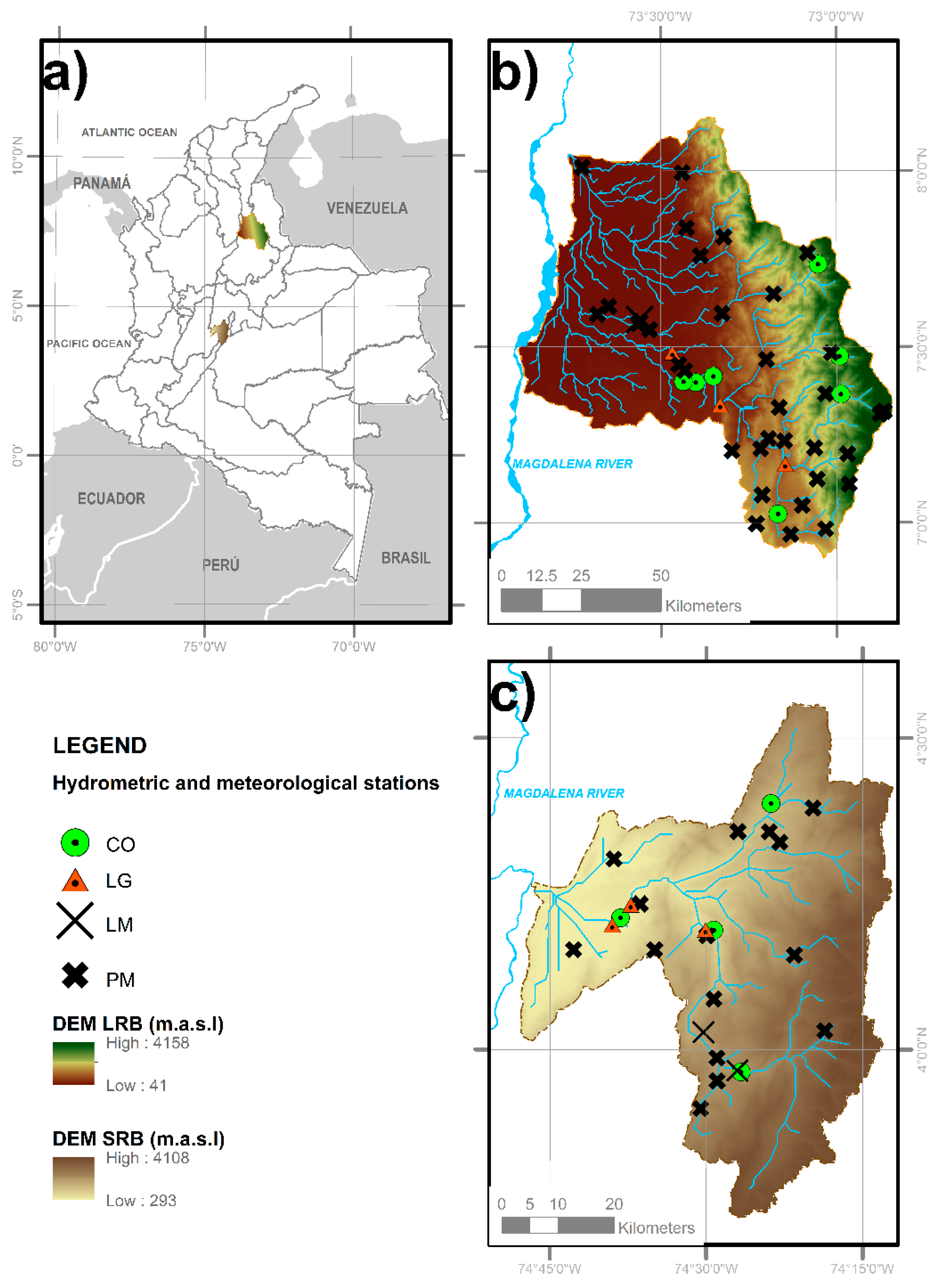
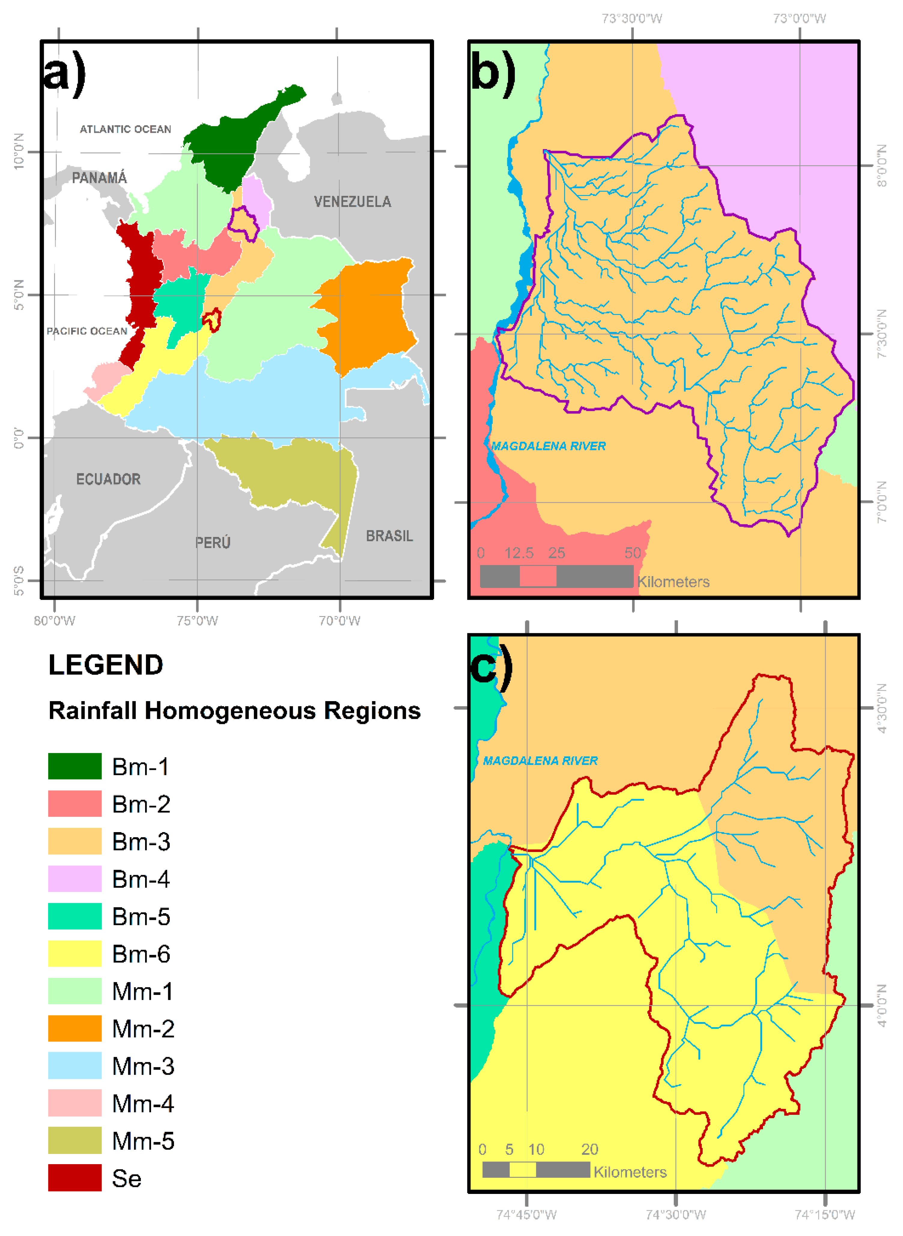
To achieve the above aims, this study compares two basins in Colombia. Monthly historic data from available hydro-meteorological stations was used to calculate the selected drought indices time series and construct point SDF curves, for subsequent regionalization and comparison between the two basins. Consistency among indices was evaluated for the same types of drought (meteorological, agricultural, and hydrological). For both basins, historical regional drought occurrences were selected and identified in the corresponding SDF curves to determine their gravity. Results of this study could contribute to regional monitoring and assessment of different types of droughts.

2. Materials and Methods

2.1. Study Areas and Datasets

The Sumapaz and Lebrija Rivers are two tributaries of the most important river in Colombia, the Magdalena River. When streamflows are analyzed, National hydrological boundaries [60], defined by the Colombian National Institute of Hydrology, Meteorology and Environmental Studies (IDEAM), locate study areas in different hydrological zones (see Figure 1a). In terms of rainfall, IDEAM has performed principal components analysis for stationarity of monthly mean rainfall, and has divided the country into 12 zones with homogenous rainfall patterns [61] (see Figure 2a). It could be noted that, despite both case studies pertaining to zones with bimodal rainfall regimes, they cannot be assumed as homogeneous, as will be described later.
In this research, monthly datasets were employed because their number of available stations and the number of missing values, for climatic and meteorological parameters, were respectively higher and lower than the ones found in daily data.
Monthly datasets were completed for missing or incomplete values using different procedures, depending on the type of data and lengths of consecutive missing months, as follows:
  • For rainfall: A weighted average of the four closest surrounding stations was used. The method used was to weight the inverse of the square of the distances between stations.
  • For temperature: Two methods were employed, depending on the number of missing values.
    If the number of missing consecutive registers were between one and six, data was calculated as a simple average for previous seven months.
    Alternatively, a multiple-regression technique was used when the number or consecutive missing registers was seven or more. In this method, only regressions with coefficients of determination of 0.5 or bigger were accepted.
  • For streamflow: Two options were evaluated. First, the use of ratings curves for hydrometric stations was tested. If stage data was unavailable for the required period, the same two techniques employed in temperature were used.
Completed datasets were analyzed for consistency using double-mass curves analysis, combined with the Pettit test applied to annually accumulated series. Corrections were applied were needed to accomplish consistency for both tests. The Pettit test was performed as indicated by Bates et al. [62], Salarijazi [63], Vezzoli et al. [64], and Yerdelen [65].
A brief description of each basin characteristics is presented below, along with a summary of the hydro-climatologic data available.

2.1.1. Sumapaz River Basin

The Sumapaz River basin (SRB) is part of the Upper Magdalena River, with an area of approximately 3085 km2 (Figure 1c). Its altitudinal variation ranges between 200 and 4050 m a.s.l. It is a vulnerable basin in terms of the potential effects on water quality from uncontrolled wastewater discharges by several municipalities [66], and the supply of drinking water to six of these ranges have an aggregate population of about 88,000 people.
Rainfall and streamflow patterns are bimodal with maximum values in April–May and October–November. Average annual rainfall varies between 1520 and 2200 mm in the western part of the basin, and between 800 and 1520 mm in the eastern part. Higher values of monthly temperature are observed in the western zone (annual average temperature of about 26 °C), followed by the central area (23.7 °C), whereas in the north and south zones average temperatures are lower (20.5 and 16.5 °C).
Specifically, the basin is divided into two different rainfall homogeneous zones (see Figure 2c): Bimodal 3 (Bm3), which contains 33% of the basin total area, and Bimodal 6 (Bm6), with the remaining 67%. Annually, both zones present two dry and wet seasons; however, the durations and the differences between extreme values vary between them. Bm3 displays a longer first dry season, with higher deficit than the second one. Wet seasons in this zone tend to behave similarly. On the other hand, Bm6 regime is characterized by a more intense second dry season than the first one, and as in the Bm3 pattern, comparable wet seasons. Figure 3a,b shows histograms of monthly mean rainfall depth for SRB stations located in Bm3 and Bm6 zones, respectively.
Observed monthly temperature, rainfall, and streamflow data of 4 weather stations, 15 rain gauges, and 5 hydrometric gaging stations located inside the basin (Figure 1c and Table 1), were available with heterogeneous record lengths.

2.1.2. Lebrija River Basin

The Lebrija River basin (LRB) is a tributary of the Middle Magdalena River, with an area of approximately 7185 km2 (Figure 1b), and elevations varying between 3050 and 70 m a.s.l. This is the fifth most stressed basin in the country, in terms of water uses and wastewater discharges [66], supplying drinking water to 4 municipalities with an aggregate population of about 603,000.
Rainfall and streamflow patterns are similar to the SRB; however, in this case, the entire basin area is contained in the Bm3 rainfall homogeneous zone (with the same features described for SRB). Figure 3c shows histograms of monthly mean rainfall depth for a typical LRB station.
In the western part of the basin, average annual rainfall ranges between 2000 and 2763 mm, and between 930 and 2000 mm in the eastern area with average annual temperature values of about 27 and 17 °C, respectively. Data of monthly temperature, rainfall, and streamflow from 7 weather stations, 34 rain gauges, and 4 streamflow stations inside the LRB were available (Figure 1b and Table 2), with different record lengths.

2.2. Drought Characterization

Droughts are frequently characterized using ‘run theory’ proposed by Yevjevich (1967) [67]. This approach enables the identification and quantification of drought characteristics, such as duration, severity, and intensity [68]. A ‘run’ is defined as a period of time in which a drought index remains over or below a threshold value (depending on the meaning of the specific index). Therefore, the principal drought characteristics that can be identified (Figure 4) are as follows:
  • Start time (ts): beginning of the drought event, equivalent to the time at which the index value crosses the threshold value.
  • Finish time (tf): time at which the index value returns to a normal level.
  • Duration (D): period between the start and finish times. During this period, the drought index is above or below the corresponding threshold value.
  • Severity (S): cumulative deficiency of drought index during the duration. It is calculated as the sum of drought index values throughout the drought duration.
  • Intensity (I): average index value over the drought duration, calculated as the severity and duration ratio.

2.3. Drought Indices (DI)

There are several drought indices, such as those proposed by Palmer (1965) [42], Gibbs & Maher (1967) [70], McKee et al. (1993) [41], Tsakiris & Vangelis (2005) [43], Tsakiris et al. (2007) [44], and Nalbantis & Tsakiris (2009) [46], among others. Some methods are based only on precipitation analysis, whilst others use different climatic series and/or rely on simplified water balances approaches [71].
Figure 1a,b display the location of stations in case studies and it is noted that most of the available data, for both study areas, came from rain gauges. As will be shown later, the regionalization procedures are highly influenced by station spatial distribution. For regional analyses, more reliability is obtained when a higher number of stations are employed [7]. For study areas, rainfall series were the most common ones, and for that reason, when selecting drought indices methods, those indices calculated using precipitation data were preferred. In this respect, the Percent of Normal Precipitation index (PN) and Standardized Precipitation Index (SPI) were selected. Moreover, it was desired to assess drought employing indices that account for water balance, despite unavailability of meteorological stations. For that reason, the Palmer indices and Reconnaissance Drought Index (RDI) were chosen. Finally, the Streamflow Drought Index (SDI) was selected to compare results obtained for hydrological drought using methods that only considered meteorological information, with a procedure that employed streamflow data.
A brief description of selected drought indices calculation procedures is given below.

2.3.1. Percent of Normal Precipitation Index (PN)

This index is one of the simplest methods of rainfall evaluation for a given location [72,73,74,75,76]. Generally, analyses using this index are useful when applied to a single region or season. The index, for a certain time period, is calculated as the quotient between actual and mean precipitation, the latter is estimated using a long historic dataset (over 30 years). In this study, this index was calculated for every weather and pluviometric station.

2.3.2. Standardized Precipitation Index (SPI)

This is probably the most frequently used tool for drought monitoring worldwide, especially at national-scales [77,78,79,80,81,82]. In 2009, the World Meteorological Organization (WMO) recommended SPI as the procedure that countries should use to track drought advance [49]. This index was calculated for all weather and pluviometric stations.
The index involves the adjustment of rainfall data to a probability distribution (generally a Gamma or Log-normal), which is transformed into a normal distribution. Therefore, index values over zero indicate rainfall depths larger than the historic median, and values below zero express the opposite. It is possible to compute this index for different time-scales, when trying to examine the effects of different drought types [57,83,84,85,86,87,88]. This index was calculated for temporal scales of 1, 3, 6, and 9 months (SPI1, SPI3, SPI6, and SPI9).

2.3.3. Moisture Anomaly Index (Z)

This index is an intermediate product in the Palmer Drought Severity Index (PDSI) calculation. One of its principal features is that it reacts almost immediately to rainfall changes [89,90,91], and its values indicate the deviation of soil moisture status from normal conditions. Research has shown that the behavior of this index is highly correlated to the SPI calculated for one month (SPI1). Data requirements, as well as the indices associated with it (PDSI and PHDI), include precipitation, temperature, geographic location, and soil field capacity. These indices were calculated only for climatic stations.

2.3.4. Palmer Drought Severity Index (PDSI)

This index is computed using an empirical expression formulated by Palmer (1965), after proposing a serial water-balance. It is calculated based on temperature and precipitation data, as well as soil water-holding capacity. The calculation procedure considers different moisture stages, including received (rainfall), stored (soil moisture), and loss (due to temperature influence) stages [92,93,94,95,96,97,98,99].

2.3.5. Reconnaissance Drought Index (RDI)

Data requirements for this method include rainfall and temperature time series, thus it was estimated only for climatic stations. Its calculation procedure considers a simplified water balance equation, where precipitation is the input and the out is potential evapotranspiration. The index accounts for the quotient between accumulated input and output values. Using a similar procedure to the one employed for the SPI index, standardized RDI is computed after normalizing the quotient dataset, which was previously adjusted to a Gamma or Log-normal distribution [44,100,101,102]. Typically, potential evapotranspiration is estimated using conventional methods, such as Penman or Thornthwaite. In this case, the second method was employed. It has been proved that the potential evapotranspiration estimation method does not have a particular influence on RDI obtained values [101].

2.3.6. Palmer Hydrological Drought Index (PHDI)

Based on the original PDSI, the PHDI includes some modifications to consider longer-term effects, related to hydrological droughts (effects to water storage, streamflow, and groundwater levels). Both Z and PHDI are computed within the calculations of PDSI.

2.3.7. Streamflow Drought Index (SDI)

This index is calculated using the same procedure as the SPI. However, instead of using rainfall, it requires streamflow data. Interpretation of SDI values is the same as for SPI [103,104,105,106]. This index was estimated using only streamflow gauging stations.

2.3.8. Drought Indices and Drought Types

As explained before, droughts can be classified depending on their impacts. Additionally, particular DI provide identification of specific drought classes. Table 3 shows the previously described calculation methodologies in relation to the drought category used for diagnosis in this study.

2.4. Point SDF Curves Construction

For both basins, frequency analyses were performed in each station for all drought indices. First, for a given index, same-duration events were identified according to Section 2.2, and annual maximum severity series for each possible duration was determined. Second, frequency analyses of these annual iso-duration severity series were performed using HYFRAN [107,108,109,110,111,112,113,114,115,116].
HYFRAN (a demo version of the software can be downloaded from https://www.wrpllc.com/books/HyfranPlus/indexhyfranplus3.html) is a software designed for hydrological frequency analysis, particularly for extreme values analysis. The software was developed at the National Institute of Scientific Research at the University of Québec. Its development received funding from the Hydro-Québec and the Natural Sciences and Engineering Research Council (NSERC). The program can be used for fitting a statistical distribution to a time series, where the observations obey the independence and identical temporal distribution hypotheses.
Parameters were estimated using the maximum-likelihood method, and goodness-of-fit was evaluated using the Chi-square test, with a significance level of 1% (implemented in HYFRAN). Gumbel, Normal, and Generalized Extreme Value (GEV) distributions adjusted relatively well to all the severity series. Frequency analyses were only performed for durations for which the number of identified events were sufficient to carry out robust adjustments, i.e., 5 or more identified events for a certain duration. Finally, the independence of the analyzed series was tested by means of the Wald-Wolfowitz test of independence, with a significance level of 5%. The last test was also implemented in HYFRAN.

2.5. SDF Curves Regionalization

Two regionalization procedures of SDF curves were employed depending on the drought index. The first procedure was applied to all indices computed from climatic information (precipitation and temperature), whereas the second was applied to the SDI, the only index calculated from streamflow data [46].
For different combinations of duration and return periods, the first procedure consisted of determining the corresponding severity value from the point SDF for each station. Then, these severity values were spatially interpolated using the Inverse Distance Weighting method (IDW) [117] implemented in ArcMap 10.4.1 (ESRI, Redlands, CA, USA) (see Figure 5), and a mean value for the whole study area was calculated. The regional SDF curve was constructed by plotting severity values in the function of the duration and return period (see Figure 6).
The second procedure considered that streamflow-based indices like SDI should be related to the tributary area. The index was calculated as a tributary-area weighted average of severities. Similar to the first procedure, computed regional severity values were plotted on regional SDF curves according to the associated duration and return period.

3. Results and Discussion

3.1. Regional SDF Curves

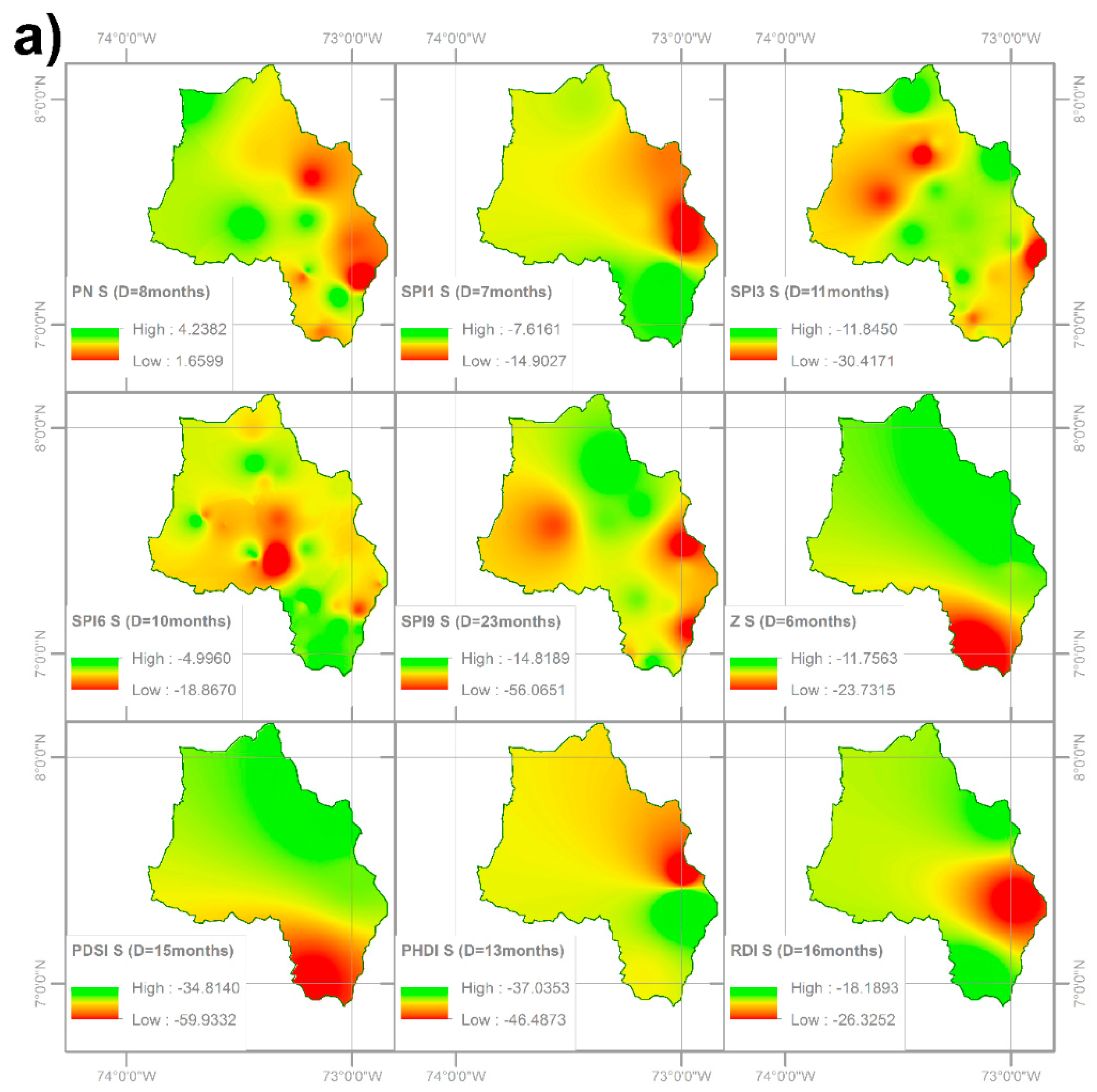
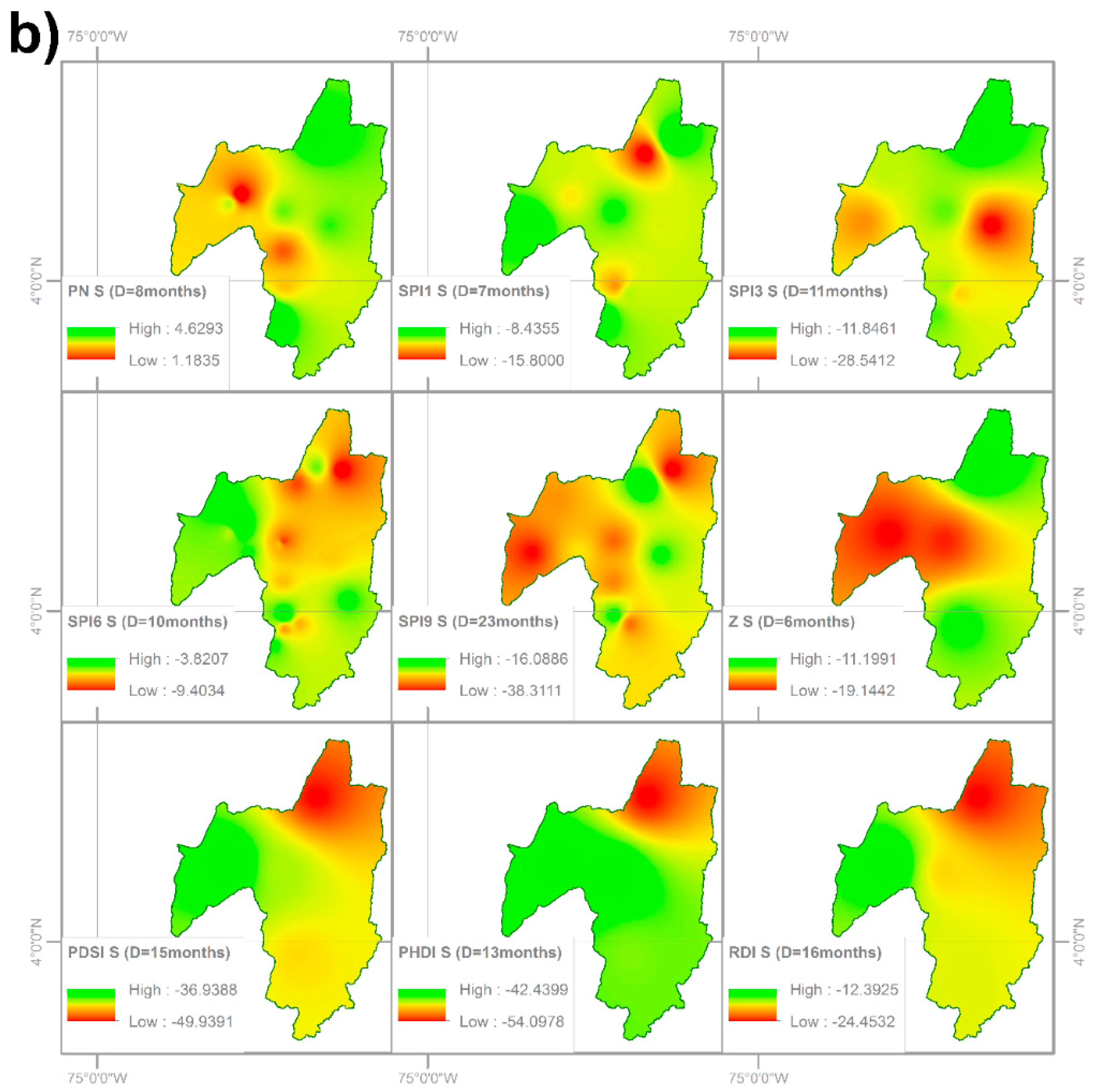
The regional SDF curves for the two case studies were compared to assess the consistency of different drought-index methods to classify the seriousness of the drought events, according to their type. As mentioned before, for the majority of DI, regionalization process was carried out by spatial interpolation of severity values obtained from point frequency analyses. In this sense, iso-severity maps constructed for maximum possible durations and return period (50 years) are displayed in Figure 5. It is notable that the location of more severe areas varies between DI methodologies. This feature is related to two relevant factors of the stations and datasets employed: (i) Variability in the length of climatic-parameters series between catchments, and between same-catchment-stations; and (ii) Differences in the spatial distribution of measuring-stations density in both case studies. The first consideration is associated with the available data for event identification and the reliability of performed frequency analysis, as well as with the regionalization of useful stations, given that each presents a diverse group of durations (according to the number of recognized drought events), and the spatial interpolation process requires a majority of stations to have a certain common duration value. The second issue is linked to the quality of the spatial interpolation procedure, which is clearly influenced by stations-proximity and catchment extent.
Additionally, it is important to mention that, as can be seen in Figure 5a, the most severe drought occurrences are concentrated on the southern and eastern regions of the LRB, except for SPI3 and SPI6, which showed higher magnitudes for stations located on the western zone of the catchment. In the SRB case study (see Figure 5b), severity spatial distribution showed lower consistency among the DI than in the LRB. Therefore, it was impossible to define a specific basin zone for which severities were shown to be larger in the SRB case study. The discrepancies described above could be fundamentally attributed to the fact that the analyzed basins were located in different hydrological zones, which implied that the particular features of the dry spells that affected them also varied. In addition, the previously-described stations and dataset characteristics, strongly influenced the spatial interpolation results.
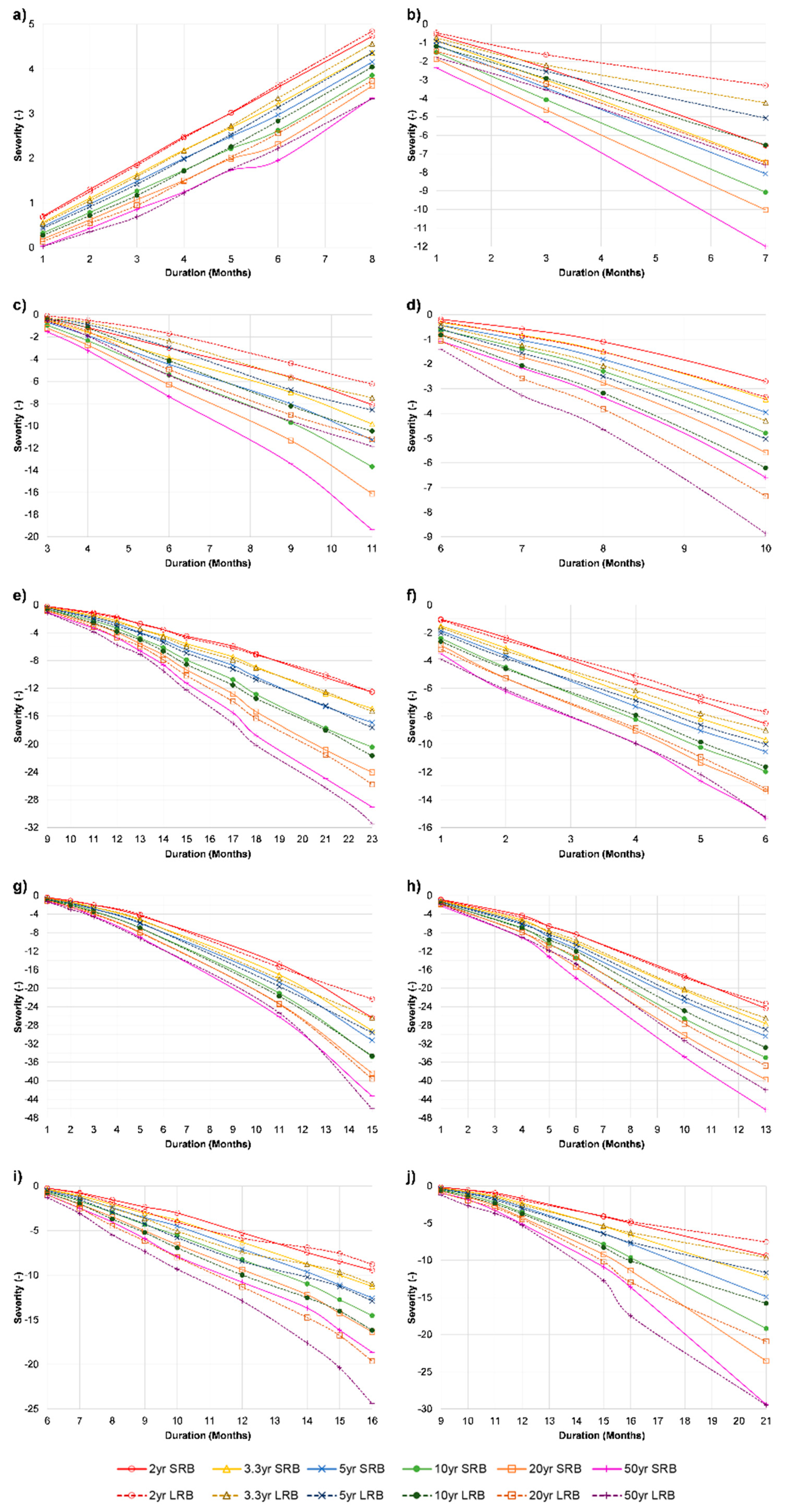
Regional SDF curves for the two study areas are depicted in Figure 6, showing that for any drought index, the regional SDF curves show similar behavior for both catchments. This fact supports the conclusion that frequency analyses maintained a distinctive relationship between severity and duration, for all drought indices. As expected, magnitudes of severities and durations for a given return period differed between catchments, which could be acceptable given that the specific hydrological attributes of both case studies (i.e., spatial distribution of stations, rainfall and temperature magnitudes, regularity of extreme event occurrences, etc.) affected the results, as mentioned before.
Specifically it was found that, for the same return period, PN, Z, and PHDI exhibited duration dependency. The first two methodologies consistently identified that the LRB presented larger gravities than the SRB for short durations (i.e., 1 to 4 months), whilst this behavior was reversed for higher durations (i.e., 5 months onward). PHDI showed that for durations between 1 and 4 months, the LRB presented larger severity values, whilst for durations of 5 months or more, the SRB surpassed it. Additionally, the LRB presented more serious occurrences identified through SPI6, SPI9, PDSI, RDI, and SDI. Remaining methodologies (SPI1 and SPI3) showed that the SRB drought events displayed larger magnitudes.
The results shown revealed the existence of a certain degree of consistency in regional-SDF curves. In this regard, PN and Z showed agreement on the identification of the study-area that displayed the most serious drought-events. Furthermore, in that particular case, concordance was reached even when differentiating outcomes depended on duration. Concurrence on the detection of the zone with the most severe same-type droughts was achieved for three more cases: (i) SPI1 and SPI3 (meteorological drought); (ii) SPI6, PDSI, and RDI (agricultural drought); and (iii) SPI9 and SDI (hydrological drought). Finally, the PHDI comparison was ambiguous given that it derived from duration–reliance results that showed no coherence with any other methodology.
According with specific DI outcomes, it was possible to define four groups of indices in terms of their compatibility between catchments: (i) PN and Z; (ii) SPI1 and SPI3; (iii) SPI6, PDSI, and RDI; and (iv) SPI9 and SDI. PHDI could not be included in any of the categories because of its lack of complete agreement with other indices that identify hydrological droughts. This grouping was useful because it facilitated the identification of DI methodologies that led to consistent results, and thus, in terms of regional planning and operation, allowed those indices with simpler calculation procedures and fewer information requirements to be selected as monitoring tools, optimizing work and resources. With this in mind, for each of the defined categories, the most appropriate operational DI would be: (i) PN; (ii) the calculation method that remains the same, so that any of the indices might be used; (iii) given that calculation methodology remains the same, data requirements were lower in SPI6 than they were in PDSI; and (iv) depending on available data (rainfall or streamflow), any of the options could be adopted.

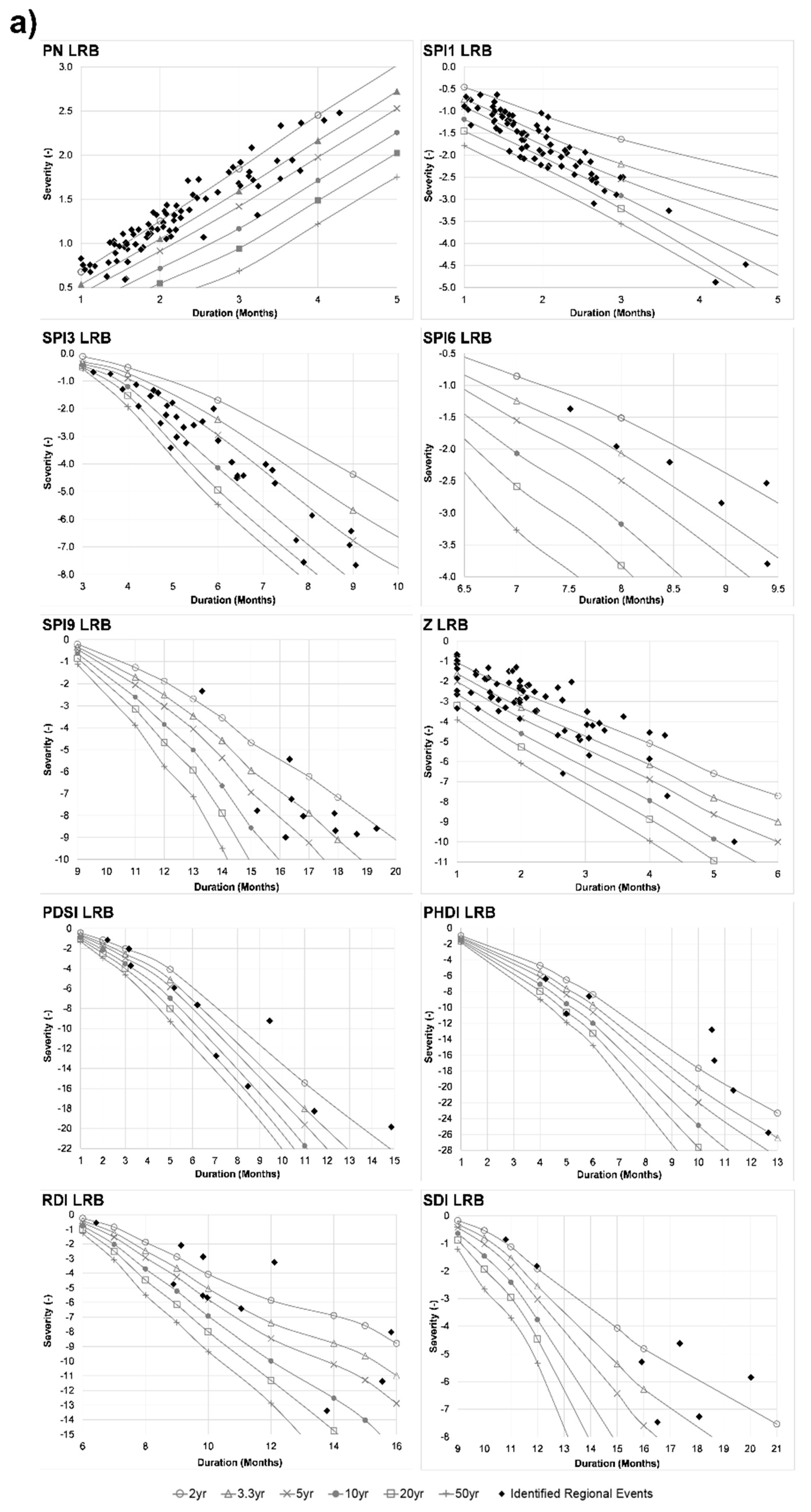
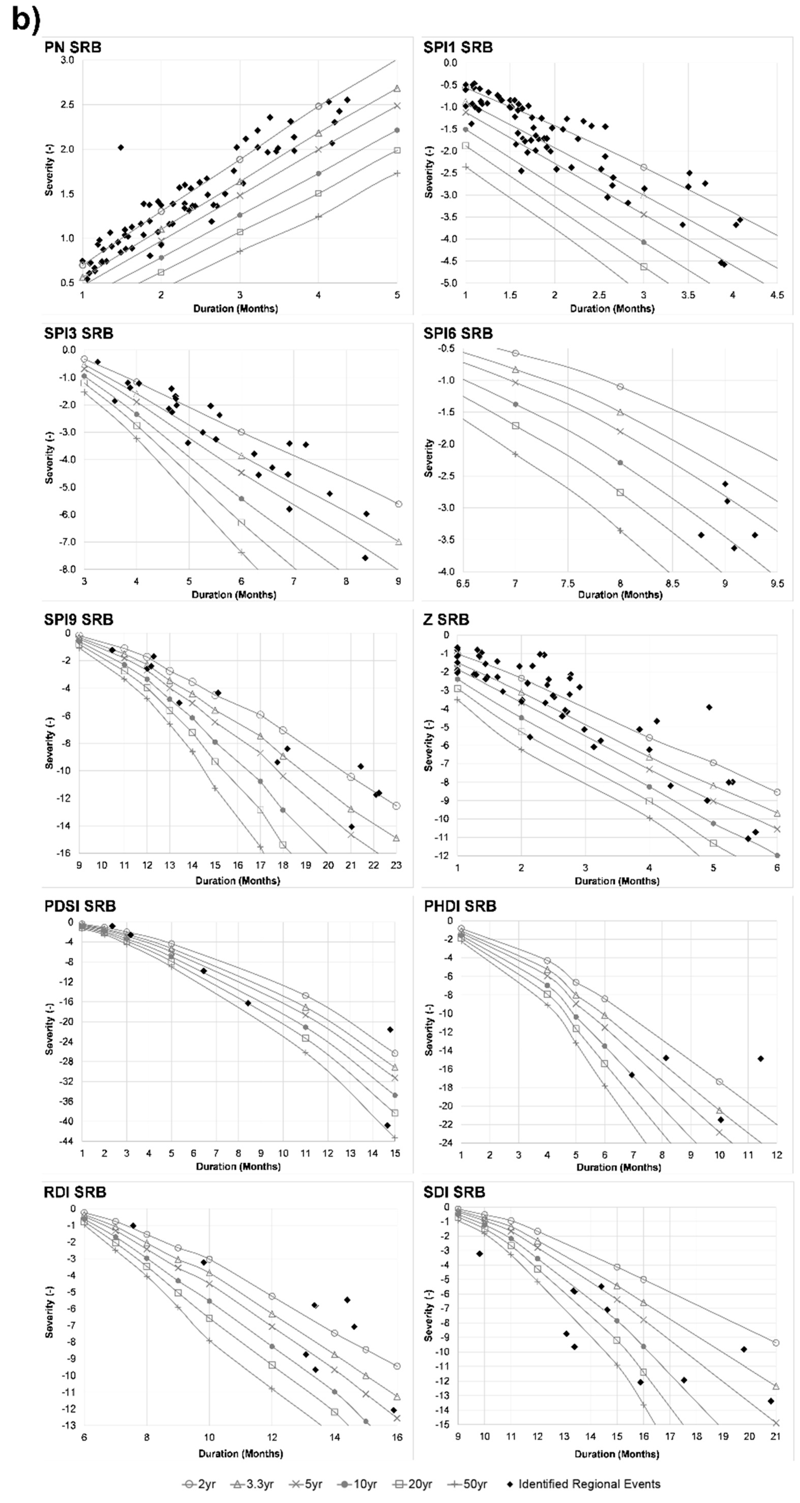
3.2. Location of Regional Drought-Events on Regional SDF Curves

Once regional SDF curves were constructed and interactions between them were explored, the next step consisted of locating historical drought-regional events, derived from datasets built from drought-indices. To identify time periods for which a significant number of stations showed drought, these occurrences were pinpointed. Once identified, spatial interpolation of drought-severities and durations was carried out, employing the same methods as SDF curves regionalization. In this way, the specific location of events over regional SDF curves were defined and their associated return period determined. Table 4 summarizes some important statistics for identified regional drought events, which were later located over constructed SDF curves. Apart from including statistics for severity and duration parameters, regional intensity measures were also included.
The results of event-location on SDF curves are presented in Figure 7a (LRB) and Figure 7b (SRB). Table 5 contains a summary of Pearson linear correlation coefficients, computed to compare the consistency of different DI methodologies to identify regional occurrences. In this respect, the SPI3 case was notable given that it could be considered as transitional between the meteorological and agricultural drought types, and for that reason, it was compared to the DI of both categories. 
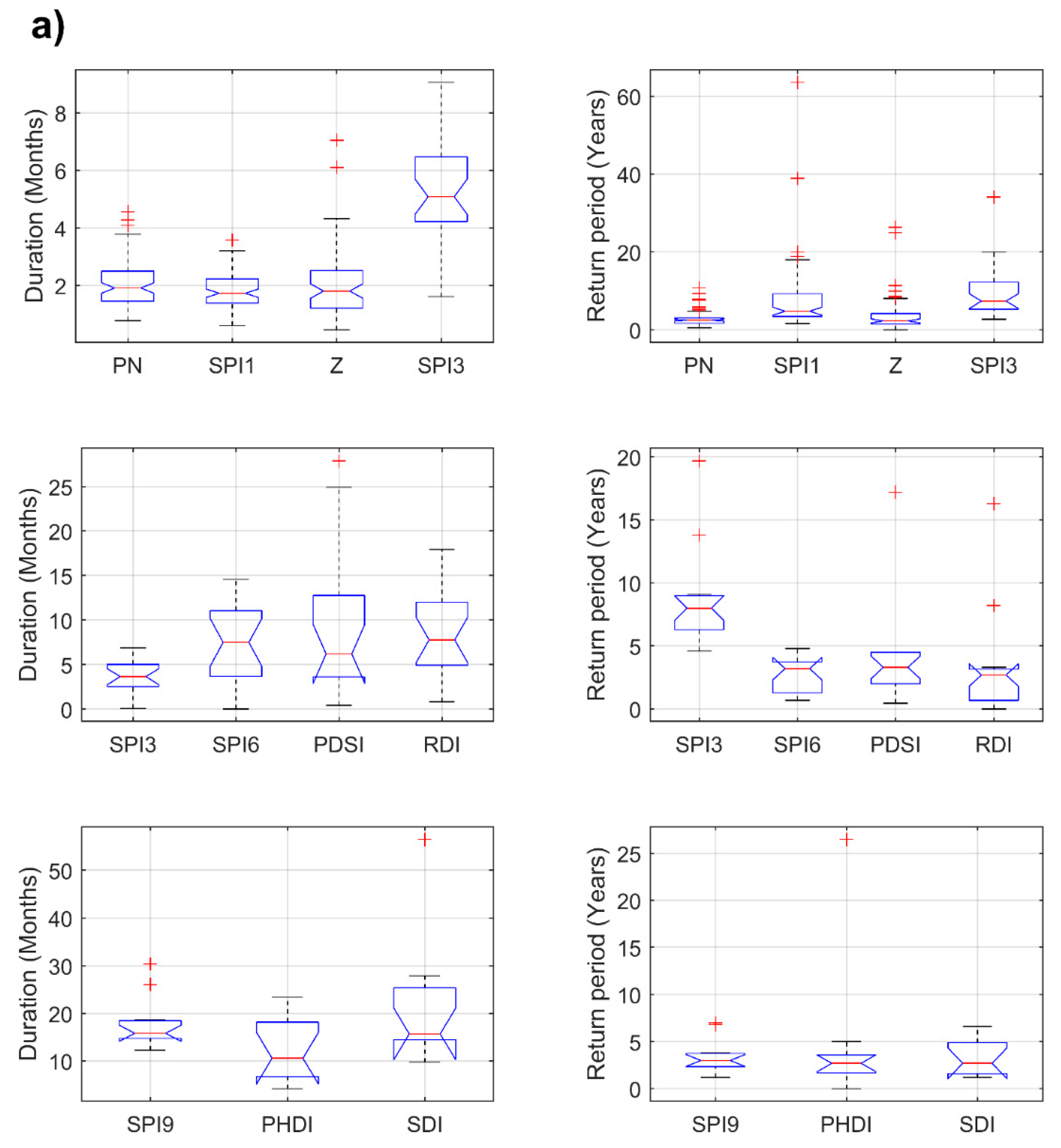
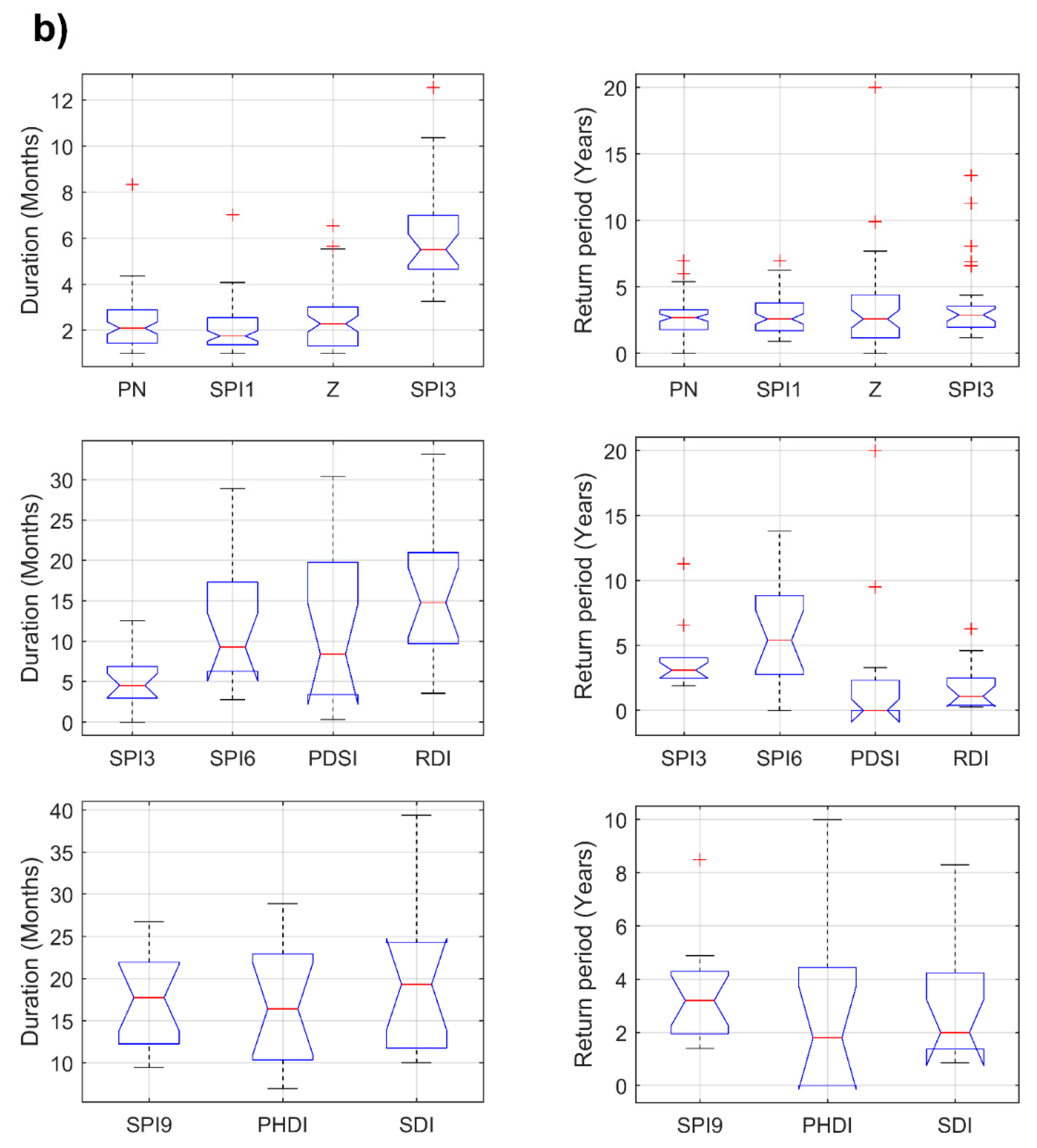
Figure 6 displays the box-whisker diagrams constructed to compare the behavior of regional event durations and return periods among different DI, for the same drought type.
Table 4 and Figure 7 identify the drought-type that displayed the highest number of regional occurrences. It was observed that meteorological drought was the most common type for both case studies (28 to 73 events in the SRB and 34 to 81 events in the LRB); agricultural drought was the second most frequent type, varying from 12 to 16 events in the SRB and from 13 to 20 events in the LRB, and the most infrequent drought type was the hydrological, with 13 to 22 episodes in the SRB and 10 to 12 in the LRB. These results were expected given the longer duration of hydrological droughts, which make them less likely to occur than the agricultural or meteorological droughts. Additionally, as will be reinforced with the results outlined below, it was found that the majority of analyzed regional events displayed return periods between 2 and 5 years, which in general terms can be considered as low.
Table 5 presents computed results after comparing duration and return period series obtained through studied DI methodologies. The main goal of this analysis was to assess the consistency of the results for different calculation procedures, with respect to the specific parameters of duration and return period series. In this sense, high values of correlation would indicate that DI methodologies could single out similar drought events, at least for duration and occurrence frequency.
Firstly, correlation values concluded that among methodologies, for both study catchments, duration series tended to be more consistent than return period series. This conclusion arose from the fact that a higher number of significant correlations were found on the duration side of Table 5 (13 of 30 evaluated correlations), than on return period side (7 of 30 evaluated correlations). Significant values were defined as those higher than 0.5, and they are shown in bold on Table 5. Secondly, it was found that higher correlations were present for the SRB than for the LRB. In the case of duration series, the SRB displayed 8 of the 13 significant correlations, whilst for frequency series, it had 5 of 7. Thirdly, it was observed that correlation coefficients for durations were significantly higher than those obtained for return periods. These results supported the conclusion that frequencies obtained through SDF regional curves, unlike durations, were highly influenced by the regionalization process. Fourthly, when analyzing relationships connected to drought type (see Table 6), the analysis found that correlations among durations tended to be higher for meteorological and hydrological droughts, than they were for agricultural droughts. In the case of frequency, the behavior was less clear, with SRB reacting in the same way as duration. Meanwhile, LRB showed larger coefficients for hydrological drought, followed by agricultural, and then meteorological. Finally, almost all of the correlation coefficients displayed a positive figure (50 of 60 evaluated correlations), which implied that for both studied parameters, correlations tended to be direct among different DI methodologies.
An analysis of the distribution of duration and return period data, obtained through different DI methodologies was carried out by means of box-and-whisker diagrams. These were constructed independently for LRB (Figure 8a) and SRB (Figure 8b). This procedure sought to evaluate consistency in duration and return period results for regional events, after characterizing both of these using regional SDF curves. For that reason, DI were grouped by drought type and each group was compared independently.
Firstly, as was previously mentioned, Box plots (Figure 8) showed that most of the identified regional events, through all the studied methodologies, displayed low return periods (between 0 and 10 years for all the DI). This could be related to the length of record employed to build the point DI series, as well as with the consistency of the identification of occurrences between stations, which classified an event as regional or not. Therefore, the importance of using datasets with a relatively long length emerged as one of the key conditions for obtaining more accurate regional analysis and identifying more high-frequency occurrences, which may be useful in the study of convenience for generated SDF areal curves.
Secondly, contrasting with the results from the Pearson correlation coefficients (Table 6), the same regional events displayed as notched box plots allowed different DI calculation procedures that were consistent with each other to be observed, with regards to duration and frequency data distribution. The box notch shows the confidence interval around the data median. Although not a formal test, if two box notches do not overlap, it is possible to consider that there is strong evidence with a 95% confidence level, that the medians of the two datasets are different. In this case, it was found that the notches corresponding to boxes of DI methodologies that identified the same type of drought tended to overlap, except for the SPI3 case which showed its transitional nature by not adjusting to the behavior of either meteorological or agricultural droughts. Moreover, it was observed that duration data distribution was more compact than frequency grouping; in other words, duration data displayed lower variability than the return period. Higher differences among DI arose from whisker length, box width, and the number and magnitude of observations outside of the whisker (i.e., possible outliers). All the mentioned discrepancies could be related with individual procedure features which determine particular data distribution, as well as with the sensitivity that durations and frequencies displayed to the regionalization process.
Finally, a relative consistency for the identification of serious events was found for both case studies using different methodologies, i.e., occurrences identified as ‘outliers’ tended to be persistent amongst calculation procedures, for both duration and frequency. Furthermore, it was found that the most severe occurrences tended to greatly impact socio-economic regional issues. For example, the previously described late 2015 and early 2016 dry period in the SRB was identified as an event with a significantly high return period by SPI3, SPI6, PDSI, and PHDI. This was not exactly an atypical value for all DI distributions, but certainly one of the higher return period values found. These results allowed this occurrence to be considered an agricultural drought for this catchment, due to the majority of methodologies that recognized it, and so it led to this conclusion. However, this drought-classification may not be taken as absolute since it also could be considered as a meteorological or hydrological-type drought, because of the SPI3 and PHDI results. The same drought episode in the LRB case study was cataloged as severe by PN, SPI3, SPI6, SPI9, and RDI. Therefore, in that case, the analyzed event could be considered transitional between a meteorological and an agricultural drought, and it also could be concluded that the occurrence was more serious than the one in the SRB, because of the number of indices that identified it. These results reaffirmed the spatial differences that the droughts exhibited when comparing distant catchments, and it confirmed that the particular characteristics of study areas defined the presence and impacts of a dry spell.

4. Conclusions

The above results, apart from classifying events according to their frequency of occurrence, facilitated the monitoring of droughts for study-regions because they supported the comparative determination of the most serious drought episodes, using not only a value of an index, but also a duration and return period associated with it. Specifically, conclusions that arose from the specific procedures applied included:
  • The SDF curves regionalization procedure was clearly influenced by measuring station density inside the study areas, as well as by the parameter’s spatial distribution. Hydrologic and soil-specific features of basins also determined the presence of drought events. Particular attention must be given to the rainfall, temperature, and streamflow series employed for the generation of DI datasets to have long enough records to generate robust point frequency analyses and accurate regional approximations.
  • When comparing both catchments generated by regional SDF curves, consistent results are found. This fact supports the supposition that distinctive correlations between severity and duration for all drought indices were conserved during the regionalization procedure. Undoubtedly, magnitudes differed between catchments because specific hydrological attributes also varied, i.e., spatial distribution of stations, rainfall and temperature magnitudes, regularity of extreme event occurrences, etc. However, it is possible to group DI methodologies that lead to consistent results for the same drought type. This is useful in terms of regional planning and operation, because it allows indices with simpler calculation procedures and fewer information requirements to be selected as monitoring tools. It is not intended to imply that one drought index methodology can be considered better than another. However, in terms of regional planning and operation, it is possible to consider that there are some methods than can be more easily applied than others. Given that the purpose of this research was the trial of procedures useful for operational purposes in Colombia, simplicity should be accomplished. The Colombian regional environmental agencies, which are in charge of designing and implementing drought response plans, do not always possess sufficient data resolution and the technical capacity to carry out complex operations. For that reason, this research was focused on simple and well-known methods, which could be easily used, despite data availability and/or specialized capabilities.
  • Regarding the location of specific historical events on regional SDF curves, the incidence of meteorological droughts was greater than the other drought types for both case studies. The duration and gravity associated with agricultural and hydrological droughts made them less frequent than those associated with rainfall reductions only. In addition, when the length of the record employed on frequency analyses was consistent, most of the identified regional events displayed low return periods. The importance of the length of the dataset used during this kind of assessment is considered as one of the decisive factors for obtaining an accurate diagnosis of regional historical occurrences.
  • When verifying the consistency of different DI methodologies regarding the identification of historical regional drought events, the obtained values of linear correlations between series of durations and frequencies affirmed that consistency tends to increase when analyzing durations instead of frequencies, for the two study-basins. This result indicated, to some extent, that the regionalization process increased variability between methodologies for frequencies, whilst for durations, its impact was not very significant (in agreement with conclusion 2). Secondly, it can be noted that consistency among DI methodologies was greater in the SRB than in the LRB. It implied that the particular features of the study region, including climatic factors, spatial density of measuring stations, and length of available datasets, influenced the coherence of calculation procedures.
  • A certain degree of consistency was found when comparing different DI methodologies, for specific drought types, for both duration and frequency parameters. It was possible to observe that medians for DIs that identify the same drought type tended to overlap with a 95% confidence level, and that occurrences identified as ‘outliers’ tended to be persistent among calculation procedures, for both of the analyzed criterion: Duration and frequency.

Author Contributions

L.P.T.R. and M.D.G. conceived and designed the methodology of this research; L.P.T.R. performed the proposed procedures, analyzed the obtained data, and wrote the paper; M.D.G. revised the paper.

Funding

This research received no external funding.

Conflicts of Interest

The authors declare no conflict of interest.

References

  1. Food and Agriculture Organization of the United Nations. The Impact of Disasters and Crises on Agriculture and Food Security, 2017; FAO: Rome, Italy, 2018; ISBN 978-92-5-130359-7. [Google Scholar]
  2. Food and Agriculture Organization of the United Nations. AQUASTAT. Available online: http://www.fao.org/nr/water/aquastat/data/query/index.html?lang=en (accessed on 27 September 2018).
  3. Yadav, S.S.; Redden, R.J.; Hatfield, J.L.; Lotze-Campen, H.; Hall, A.E. Crop Adaptation to Climate Change; Wiley-Blackwell: Oxford, UK, 2011; ISBN 978-0-470-96092-9. [Google Scholar]
  4. Espinoza, G.; Hajek, E. Riesgos climáticos: Evidencias en Chile central. In Ecología del Paisaje en Chile Central: Estudios Sobre sus Espacios Montañosos; Fuentes, E.R., Prenafeta, S., Eds.; Universidad Católica de Chile: Santiago, Chile, 1998; pp. 41–51. [Google Scholar]
  5. Oxford Bussiness Group (OBG). The Report: Colombia 2016; OBG: London, UK, 2016. [Google Scholar]
  6. Richard, Y.; Fauchereau, N.; Poccard, I.; Rouault, M.; Trzaska, S. 20th century droughts in southern Africa: Spatial and temporal variability, teleconnections with oceanic and atmospheric conditions. Int. J. Climatol. 2001, 21, 873–885. [Google Scholar] [CrossRef]
  7. Brown, J.F.; Wardlow, B.D.; Tadesse, T.; Hayes, M.J.; Reed, B.C. The vegetation drought response index (VegDRI): A new integrated approach for monitoring drought stress in vegetation. GISci. Remote Sens. 2008, 45, 16–46. [Google Scholar] [CrossRef]
  8. Raziei, T.; Saghafian, B.; Paulo, A.A.; Pereira, L.S.; Bordi, I. Spatial patterns and temporal variability of drought in Western Iran. Water Resour. Manag. 2009, 23, 439–455. [Google Scholar] [CrossRef]
  9. Santos, J.F.; Pulido-Calvo, I.; Portela, M.M. Spatial and temporal variability of droughts in Portugal. Water Resour. Res. 2010, 46. [Google Scholar] [CrossRef] [Green Version]
  10. Martins, D.S.; Raziei, T.; Paulo, A.A.; Pereira, L.S. Spatial and temporal variability of precipitation and drought in Portugal. Nat. Hazards Earth Syst. Sci. 2012, 12, 1493–1501. [Google Scholar] [CrossRef] [Green Version]
  11. Wang, H.; Chen, Y.; Pan, Y.; Li, W. Spatial and temporal variability of drought in the arid region of China and its relationships to teleconnection indices. J. Hydrol. 2015, 523, 283–296. [Google Scholar] [CrossRef]
  12. Wilhite, D.A.; Glantz, M.H. Understanding: The drought phenomenon: The role of definitions. Water Int. 1985, 10, 111–120. [Google Scholar] [CrossRef]
  13. Mishra, A.K.; Singh, V.P. A review of drought concepts. J. Hydrol. 2010, 391, 202–216. [Google Scholar] [CrossRef]
  14. Zhang, Q.; Li, J.; Singh, V.P.; Bai, Y. SPI-based evaluation of drought events in Xinjiang, China. Nat. Hazards 2012, 64, 481–492. [Google Scholar] [CrossRef]
  15. Paparrizos, S.; Maris, F.; Matzarakis, A. Mapping of drought for Sperchios River basin in central Greece. Hydrol. Sci. J. 2016, 1–11. [Google Scholar] [CrossRef]
  16. Dabanlı, İ.; Mishra, A.K.; Şen, Z. Long-term spatio-temporal drought variability in Turkey. J. Hydrol. 2017, 552, 779–792. [Google Scholar] [CrossRef]
  17. Kaluba, P.; Verbist, K.M.J.; Cornelis, W.M.; Van Ranst, E. Spatial mapping of drought in Zambia using regional frequency analysis. Hydrol. Sci. J. 2017, 62, 1825–1839. [Google Scholar] [CrossRef]
  18. Bayissa, Y.A.; Moges, S.A.; Xuan, Y.; Van Andel, S.J.; Maskey, S.; Solomatine, D.P.; Griensven, A.V.; Tadesse, T. Spatio-temporal assessment of meteorological drought under the influence of varying record length: The case of Upper Blue Nile Basin, Ethiopia. Hydrol. Sci. J. 2015, 60, 1–16. [Google Scholar] [CrossRef]
  19. Ganguli, P.; Ganguly, A.R. Space-time trends in U.S. meteorological droughts. J. Hydrol. Reg. Stud. 2016, 8, 235–259. [Google Scholar] [CrossRef]
  20. Kazemzadeh, M.; Malekian, A. Spatial characteristics and temporal trends of meteorological and hydrological droughts in northwestern Iran. Nat. Hazards 2016, 80, 191–210. [Google Scholar] [CrossRef]
  21. Dash, B.K.; Rafiuddin, M.; Khanam, F.; Islam, M.N. Characteristics of meteorological drought in Bangladesh. Nat. Hazards 2012, 64, 1461–1474. [Google Scholar] [CrossRef]
  22. Li, B.; Liang, Z.; Yu, Z.; Acharya, K. Evaluation of drought and wetness episodes in a cold region (Northeast China) since 1898 with different drought indices. Nat. Hazards 2014, 71, 2063–2085. [Google Scholar] [CrossRef]
  23. Yacoub, E.; Tayfur, G. Evaluation and assessment of meteorological drought by different methods in Trarza Region, Mauritania. Water Resour. Manag. 2017, 31, 825–845. [Google Scholar] [CrossRef]
  24. Wong, G.; van Lanen, H.A.J.; Torfs, P.J.J.F. Probabilistic analysis of hydrological drought characteristics using meteorological drought. Hydrol. Sci. J. 2013, 58, 253–270. [Google Scholar] [CrossRef] [Green Version]
  25. Lin, Q.; Wu, Z.; Singh, V.P.; Sadeghi, S.H.R.; He, H.; Lu, G. Correlation between hydrological drought, climatic factors, reservoir operation, and vegetation cover in the Xijiang Basin, South China. J. Hydrol. 2017, 549, 512–524. [Google Scholar] [CrossRef]
  26. Bonaccorso, B.; Bordi, I.; Cancelliere, A.; Rossi, G.; Sutera, A. Spatial variability of drought: An analysis of the SPI in Sicily. Water Resour. Manag. 2003, 17, 273–296. [Google Scholar] [CrossRef]
  27. Wu, J.; Chen, X.; Yao, H.; Gao, L.; Chen, Y.; Liu, M. Non-linear relationship of hydrological drought responding to meteorological drought and impact of a large reservoir. J. Hydrol. 2017, 551, 495–507. [Google Scholar] [CrossRef]
  28. Pandey, R.P.; Mishra, S.K.; Singh, R.; Ramasastri, K.S. Streamflow drought severity analysis of Betwa river system (India). Water Resour. Manag. 2008, 22, 1127–1141. [Google Scholar] [CrossRef]
  29. Jeong, S.; Yu, I.; Felix, M.L.A.; Kim, S.; Oh, K. Drought assessment for real-time hydrologic drought index of the Nakdong River Basin in Korea. Desalin. Water Treat. 2014, 52, 2826–2832. [Google Scholar] [CrossRef]
  30. Razmkhah, H. Comparing threshold level methods in development of stream flow drought severity-duration-frequency curves. Water Resour. Manag. 2017, 31, 4045–4061. [Google Scholar] [CrossRef]
  31. Vu, M.T.; Vo, N.D.; Gourbesville, P.; Raghavan, S.V.; Liong, S.-Y. Hydro-meteorological drought assessment under climate change impact over the Vu Gia–Thu Bon River Basin, Vietnam. Hydrol. Sci. J. 2017, 62, 1654–1668. [Google Scholar] [CrossRef]
  32. Farrar, T.J.; Nicholson, S.E.; Lare, A.R. The Influence of soil type on the relationships between NDVI, rainfall, and soil moisture in semiarid Botswana. II. NDVI response to soil moisture. Remote Sens. Environ. 1994, 50, 121–133. [Google Scholar] [CrossRef]
  33. Wang, J.; Price, K.P.; Rich, P.M. Spatial patterns of NDVI in response to precipitation and temperature in the central Great Plains. Int. J. Remote Sens. 2001, 22, 3827–3844. [Google Scholar] [CrossRef]
  34. Ji, L.; Peters, A.J. Assessing vegetation response to drought in the northern Great Plains using vegetation and drought indices. Remote Sens. Environ. 2003, 87, 85–98. [Google Scholar] [CrossRef]
  35. Wan, Z.; Wang, P.; Li, X. Using MODIS land surface temperature and normalized difference vegetation index products for monitoring drought in the southern Great Plains, USA. Int. J. Remote Sens. 2004, 25, 61–72. [Google Scholar] [CrossRef]
  36. Jain, S.K.; Keshri, R.; Goswami, A.; Sarkar, A.; Chaudhry, A. Identification of drought-vulnerable areas using NOAA AVHRR data. Int. J. Remote Sens. 2009, 30, 2653–2668. [Google Scholar] [CrossRef]
  37. Quiring, S.M.; Ganesh, S. Evaluating the utility of the Vegetation Condition Index (VCI) for monitoring meteorological drought in Texas. Agric. For. Meteorol. 2010, 150, 330–339. [Google Scholar] [CrossRef]
  38. Bajgain, R.; Xiao, X.; Wagle, P.; Basara, J.; Zhou, Y. Sensitivity analysis of vegetation indices to drought over two tallgrass prairie sites. ISPRS J. Photogramm. Remote Sens. 2015, 108, 151–160. [Google Scholar] [CrossRef]
  39. Vicente-Serrano, S.M.; Beguería, S.; Lorenzo-Lacruz, J.; Julio, J.; López-Moreno, J.I.; Azorín-Molina, C.; Revuelto, J.; Sánchez-Lorenzo, A. Análisis Comparativo de Diferentes Índices de Sequía para Aplicaciones Ecológicas, Agrícolas e Hidrológicas; Asociación Española de Climatología (AEC): Salamanca, Spain, 2012; pp. 679–690.
  40. Hayes, M.J. Drought indices. Intermt. West Clim. Summ. 2007, 3, 2–6. [Google Scholar]
  41. McKee, T.B.; Doesken, N.J.; Kleist, J. The Relationship of Drought Frequency and Duration to Time Scales; American Meteorological Society: Anaheim, CA, USA, 1993; p. 6. [Google Scholar]
  42. Palmer, W. Meteorological Drought; Research Paper; U.S. Weather Bureau: Washington, DC, USA, 1965; p. 65.
  43. Tsakiris, G.; Vangelis, H. Establishing a drought index incorporating evapotranspiration. Eur. Water 2005, 9, 3–11. [Google Scholar]
  44. Tsakiris, G.; Pangalou, D.; Vangelis, H. Regional drought assessment based on the Reconnaissance Drought Index (RDI). Water Resour. Manag. 2007, 21, 821–833. [Google Scholar] [CrossRef]
  45. Vicente-Serrano, S.M.; Beguería, S.; López-Moreno, J.I. A multiscalar drought index sensitive to global warming: The standardized precipitation evapotranspiration index. J. Clim. 2010, 23, 1696–1718. [Google Scholar] [CrossRef]
  46. Nalbantis, I.; Tsakiris, G. Assessment of hydrological drought revisited. Water Resour. Manag. 2009, 23, 881–897. [Google Scholar] [CrossRef]
  47. Onyutha, C. On rigorous drought assessment using daily time scale: Non-stationary frequency analyses, revisited concepts, and a new method to yield non-parametric indices. Hydrology 2017, 4, 48. [Google Scholar] [CrossRef]
  48. Chow, V.T. Handbook of Applied Hydrology; McGraw Hill: New York, NY, USA, 1964. [Google Scholar]
  49. World Meteorological Organization. Guide to Hydrological Practices, 6th ed.; WMO: Geneva, Switzerland, 2008; ISBN 978-92-63-10168-6. [Google Scholar]
  50. Dalezios, N.R.; Loukas, A.; Vasiliades, L.; Liakopoulos, E. Severity-duration-frequency analysis of droughts and wet periods in Greece. Hydrol. Sci. J. 2000, 45, 751–769. [Google Scholar] [CrossRef] [Green Version]
  51. Todisco, F.; Mannocchi, F.; Vergni, L. Severity–duration–frequency curves in the mitigation of drought impact: An agricultural case study. Nat. Hazards 2013, 65, 1863–1881. [Google Scholar] [CrossRef]
  52. Janga Reddy, M.; Ganguli, P. Application of copulas for derivation of drought severity–duration–frequency curves. Hydrol. Process. 2012, 26, 1672–1685. [Google Scholar] [CrossRef]
  53. Halwatura, D.; Lechner, A.M.; Arnold, S. Drought severity–duration–frequency curves: A foundation for risk assessment and planning tool for ecosystem establishment in post-mining landscapes. Hydrol. Earth Syst. Sci. 2015, 19, 1069–1091. [Google Scholar] [CrossRef]
  54. Rahmat, S.; Jayasuriya, N.; Bhuiyan, M. Development of drought severity–duration–frequency curves in Victoria, Australia. Austral. J. Water Resour. 2015, 19. [Google Scholar] [CrossRef]
  55. Saghafian, B.; Shokoohi, A.; Raziei, T. Drought spatial analysis and development of severity–duration–frequency curves for an arid region. In Hydrology of the Mediterranean and Semiarid Regions; IAHS Publ.: Montpellier, France, 2003; Volume 278, pp. 305–311. [Google Scholar]
  56. Yoo, C.; Kim, D.; Kim, T.-W.; Hwang, K.-N. Quantification of drought using a rectangular pulses Poisson process model. J. Hydrol. 2008, 355, 34–48. [Google Scholar] [CrossRef]
  57. Vicente-Serrano, S.M. Spatial and temporal analysis of droughts in the Iberian Peninsula (1910–2000). Hydrol. Sci. J. 2006, 51, 83–97. [Google Scholar] [CrossRef] [Green Version]
  58. Zhu, G.; Yang, L.; Qin, D.; Tong, H.; Liu, Y.; Li, J. Spatial and temporal variation of drought index in a typical steep alpine terrain in Hengduan Mountains. J. Mt. Sci. 2016, 13, 1186–1199. [Google Scholar] [CrossRef]
  59. Ayantobo, O.O.; Li, Y.; Song, S.; Yao, N. Spatial comparability of drought characteristics and related return periods in mainland China over 1961–2013. J. Hydrol. 2017, 550, 549–567. [Google Scholar] [CrossRef]
  60. Instituto de Hidrología, Meteorología y Estudios Ambientales (IDEAM). Zonificación y Codificación de Unidades Hidrográficas e Hidrogeológicas de Colombia; IDEAM: Bogotá, Colombia, 2013.
  61. Guzmán, D.; Ruiz, J.F.; Cadena, M. Regionalización de Colombia Según la Estacionalidad de la Precipitación Media Mensual, a Través de Análisis de Componentes Principales (ACP); Instituto de Hidrología, Meteorología y Estudios Ambientales (IDEAM): Bogotá, Colombia, 2014.
  62. Bates, B.C.; Chandler, R.E.; Bowman, A.W. Trend estimation and change point detection in individual climatic series using flexible regression methods: Trend and Change Point Detection. J. Geophys. Res. Atmos. 2012, 117. [Google Scholar] [CrossRef]
  63. Salarijazi, M. Trend and change-point detection for the annual stream-flow series of the Karun River at the Ahvaz hydrometric station. Afr. J. Agric. Res. 2012, 7. [Google Scholar] [CrossRef]
  64. Vezzoli, R.; Pecora, S.; Zenoni, E.; Tonelli, F. Data analysis to detect inhomogeneity, change points, trends in observations: an application to Po river discharge extremes. SSRN Electron. J. 2012. [Google Scholar] [CrossRef]
  65. Yerdelen, C. Change point of river stream OW in Turkey. Sci. Iran. 2014, 21, 306–317. [Google Scholar]
  66. Instituto de Hidrología, Meteorología y Estudios Ambientales (IDEAM). Estudio Nacional del Agua 2014; IDEAM: Bogotá, Colombia, 2015; ISBN 978-958-8067-70-4.
  67. Yevjevich, V. An objective approach to definitions and investigations of continental hydrologic droughts. J. Hydrol. 1969, 7, 353. [Google Scholar] [CrossRef]
  68. Chang, J.; Li, Y.; Wang, Y.; Yuan, M. Copula-based drought risk assessment combined with an integrated index in the Wei River Basin, China. J. Hydrol. 2016, 540, 824–834. [Google Scholar] [CrossRef]
  69. U.S. Geological Survey (USGS). 3sec GRID: Void-Filled DEM; USGS: Reston, VA, USA, 2013.
  70. Gibbs, W.J.; Maher, J.V. Rainfall Deciles as Drought Indicators; Bulletin; Commonwealth Bureau of Meteorology: Melbourne, Australia, 1967; p. 84.
  71. Hurtado, G.; Cadena, M. Aplicación de índices de sequía en Colombia. Meteorol. Colomb. 2002, 5, 131–137. [Google Scholar]
  72. Morid, S.; Smakhtin, V.; Moghaddasi, M. Comparison of seven meteorological indices for drought monitoring in Iran. Int. J. Climatol. 2006, 26, 971–985. [Google Scholar] [CrossRef] [Green Version]
  73. Quiring, S.M. Developing objective operational definitions for monitoring drought. J. Appl. Meteorol. Climatol. 2009, 48, 1217–1229. [Google Scholar] [CrossRef]
  74. Quiring, S.M. Monitoring drought: An evaluation of meteorological drought indices. Geogr. Compass 2009, 3, 64–88. [Google Scholar] [CrossRef]
  75. Nikbakht, J.; Tabari, H.; Talaee, P.H. Streamflow drought severity analysis by percent of normal index (PNI) in northwest Iran. Theor. Appl. Climatol. 2013, 112, 565–573. [Google Scholar] [CrossRef]
  76. Gocic, M.; Trajkovic, S. Spatiotemporal characteristics of drought in Serbia. J. Hydrol. 2014, 510, 110–123. [Google Scholar] [CrossRef]
  77. Komuscu, A.U. Using the SPI to analyze spatial and temporal patterns of drought in Turkey. Drought Netw. News (1994–2001) 1999, 11, 8. [Google Scholar]
  78. Agnew, C.T. Using the SPI to identify drought. Drought Netw. News (1994–2001) 2000, 12, 8. [Google Scholar]
  79. Livada, I.; Assimakopoulos, V.D. Spatial and temporal analysis of drought in Greece using the Standardized Precipitation Index (SPI). Theor. Appl. Climatol. 2007, 89, 143–153. [Google Scholar] [CrossRef]
  80. Łabędzki, L. Estimation of local drought frequency in central Poland using the standardized precipitation index SPI. Irrig. Drain. 2007, 56, 67–77. [Google Scholar] [CrossRef]
  81. Chortaria, C.; Karavitis, C.A.; Alexandris, S. Development of the SPI Drought Index for Greece Using Geo-Statistical Methods; Republic of Macedonia: Ohrid, Republic of Macedonia, 2010; pp. 1–11. [Google Scholar]
  82. Belayneh, A.; Adamowski, J.; Khalil, B.; Ozga-Zielinski, B. Long-term SPI drought forecasting in the Awash River Basin in Ethiopia using wavelet neural network and wavelet support vector regression models. J. Hydrol. 2014, 508, 418–429. [Google Scholar] [CrossRef]
  83. Seiler, R.A.; Hayes, M.; Bressan, L. Using the standardized precipitation index for flood risk monitoring. Int. J. Climatol. 2002, 22, 1365–1376. [Google Scholar] [CrossRef] [Green Version]
  84. Rouault, M.; Richard, Y. Intensity and spatial extension of drought in South Africa at different time scales. Water SA 2004, 29, 489–500. [Google Scholar] [CrossRef]
  85. Vicente-Serrano, S.M.; Lopez-Moreno, J.I. Hydrological response to different time scales of climatological drought: An evaluation of the Standardized Precipitation Index in a mountainous Mediterranean basin. Hydrol. Earth Syst. Sci. 2005, 9, 523–533. [Google Scholar] [CrossRef] [Green Version]
  86. Vicente-Serrano, S.M.; Cuadrat-Prats, J.M.; Romo, A. Early prediction of crop production using drought indices at different time-scales and remote sensing data: Application in the Ebro Valley (north-east Spain). Int. J. Remote Sens. 2006, 27, 511–518. [Google Scholar] [CrossRef]
  87. Pasho, E.; Camarero, J.J.; de Luis, M.; Vicente-Serrano, S.M. Impacts of drought at different time scales on forest growth across a wide climatic gradient in north-eastern Spain. Agric. For. Meteorol. 2011, 151, 1800–1811. [Google Scholar] [CrossRef]
  88. Potop, V.; Možný, M.; Soukup, J. Drought evolution at various time scales in the lowland regions and their impact on vegetable crops in the Czech Republic. Agric. For. Meteorol. 2012, 156, 121–133. [Google Scholar] [CrossRef]
  89. Sakamoto, C.M. The Z-index as a variable for crop yield estimation. Agric. Meteorol. 1978, 19, 305–313. [Google Scholar] [CrossRef]
  90. Karl, T.R. The sensitivity of the Palmer drought severity index and Palmer’s Z-index to their calibration coefficients including potential evapotranspiration. J. Appl. Meteorol. Climatol. 1986, 25, 77–86. [Google Scholar] [CrossRef]
  91. Loukas, A.; Vasiliades, L.; Dalezios, N.R. Hydroclimatic variability of regional droughts in greece using the Palmer Moisture Anomaly index. Hydrol. Res. 2002, 33, 425–442. [Google Scholar] [CrossRef]
  92. Guttman, N.B.; Wallis, J.R.; Hosking, J.R.M. Spatial comparability of the Palmer drought severity index. J. Am. Water Resour. Assoc. 1992, 28, 1111–1119. [Google Scholar] [CrossRef]
  93. Briffa, K.R.; Jones, P.D.; Hulme, M. Summer moisture variability across Europe, 1892–1991: An analysis based on the palmer drought severity index. Int. J. Climatol. 1994, 14, 475–506. [Google Scholar] [CrossRef]
  94. Guttman, N.B. Comparing the palmer drought index and the standarized precipitation index. J. Am. Water Resour. Assoc. 1998, 34, 113–121. [Google Scholar] [CrossRef]
  95. Lohani, V.K.; Loganathan, G.V.; Mostaghimi, S. Long-term analysis and short-term forecasting of dry spells by Palmer Drought Severity Index. Hydrol. Res. 1998, 29, 21–40. [Google Scholar] [CrossRef]
  96. Hu, Q.; Willson, G.D. Effects of temperature anomalies on the Palmer Drought Severity Index in the central United States. Int. J. Climatol. 2000, 20, 1899–1911. [Google Scholar] [CrossRef] [Green Version]
  97. Dai, A.; Trenberth, K.E.; Qian, T. A global dataset of Palmer Drought Severity index for 1870–2002: relationship with soil moisture and effects of surface warming. J. Hydrometeorol. 2004, 5, 1117–1130. [Google Scholar] [CrossRef]
  98. Li, J.; Chen, F.; Cook, E.R.; Gou, X.; Zhang, Y. Drought reconstruction for North Central China from tree rings: The value of the Palmer drought severity index. Int. J. Climatol. 2007, 27, 903–909. [Google Scholar] [CrossRef]
  99. Dai, A. Characteristics and trends in various forms of the Palmer Drought Severity Index during 1900–2008. J. Geophys. Res. 2011, 116. [Google Scholar] [CrossRef] [Green Version]
  100. Pashiardis, S.; Michaelides, S. Implementation of the standardized precipitation index (SPI) and the reconnaissance drought index (RDI) for regional drought assessment: A case study for Cyprus. Eur. Water 2008, 23–24, 57–65. [Google Scholar]
  101. Vangelis, H.; Tigkas, D.; Tsakiris, G. The effect of PET method on Reconnaissance Drought Index (RDI) calculation. J. Arid Environ. 2013, 88, 130–140. [Google Scholar] [CrossRef]
  102. Kousari, M.R.; Dastorani, M.T.; Niazi, Y.; Soheili, E.; Hayatzadeh, M.; Chezgi, J. Trend Detection of Drought in Arid and Semi-Arid Regions of Iran Based on Implementation of Reconnaissance Drought Index (RDI) and Application of Non-Parametrical Statistical Method. Water Resour. Manag. 2014, 28, 1857–1872. [Google Scholar] [CrossRef]
  103. Nalbantis, I. Evaluation of a Hydrological Drought Index. Eur. Water 2008, 23–24, 67–77. [Google Scholar]
  104. Dehghani, M.; Saghafian, B.; Nasiri Saleh, F.; Farokhnia, A.; Noori, R. Uncertainty analysis of streamflow drought forecast using artificial neural networks and Monte-Carlo simulation. Int. J. Climatol. 2014, 34, 1169–1180. [Google Scholar] [CrossRef]
  105. Tabari, H.; Nikbakht, J.; Hosseinzadeh Talaee, P. Hydrological drought assessment in Northwestern Iran based on streamflow drought index (SDI). Water Resour. Manag. 2013, 27, 137–151. [Google Scholar] [CrossRef]
  106. Hong, X.; Guo, S.; Zhou, Y.; Xiong, L. Uncertainties in assessing hydrological drought using streamflow drought index for the upper Yangtze River basin. Stoch. Environ. Res. Risk Assess. 2015, 29, 1235–1247. [Google Scholar] [CrossRef]
  107. Chair in Statistical Hydrology. INRS-ETE HYFRAN; Chaire Indusrielle Hydro-Québec/CRSNG en Hydrologie Statistique/Institut National de la Recherche Scientifique (INRS)/Centre Eau, Terre et Environnement: Montréal, QC, Canada, 2002. [Google Scholar]
  108. Aboodi, A.H.A. Probability analysis of extreme monthly rainfall in Baghdad city, middle of Iraq. Basrah J. Eng. Sci. 2014, 14, 1–12. [Google Scholar]
  109. Dawood, A.S. Probability analysis of extreme monthly rainfall in Mosul City, North of Iraq. March Bull. 2009, 4, 60–74. [Google Scholar]
  110. Restle, E.M.; El Adlouni, S.; Bobée, B.; Ouarda, T.B. Le Test GPD et son Implémentation Dans le Logiciel HYFRAN PRO; Chaire Indusrielle Hydro-Québec/CRSNG en Hydrologie Statistique/Institut National de la Recherche Scientifique (INRS)/Centre Eau, Terre et Environnement: Montréal, QC, Canada, 2004; p. 47. [Google Scholar]
  111. Bobée, B.; Des Groseilliers, L. Ajustement des Distributions Pearson Type 3, Gamma, Gamma Généralisée, Log-Pearson Type 3 et Log-Gamma; INRS-Eau, Université du Québec: Montréal, QC, Canada, 1985; p. 154. [Google Scholar]
  112. Paria Christ Jesus Barriga; Lima Hernani Mota. O uso de Geotêxtil para o Controle de Drenagem de Água de Superfície—A Solução Utilizada para Fechamento Adequado de uma Pilha Estéril; Associação Brasileira de Mecânica dos Solos e Engenharia Geotécnica (ABMS): Belo Horizonte, Brasil, 2016. [Google Scholar]
  113. Perreault, L.; Bobée, B.; Legendre, P. Rapport Général du Logiciel AJUSTE II: Théorie et Application; INRS-Eau, Université du Québec: Montréal, QC, Canada, 1994; p. 102. [Google Scholar]
  114. El Adlouni, S.; Bobée, B. Analyse Fréquentielle avec le Logiciel HYFRAN-PLUS; Chaire Indusrielle Hydro-Québec/CRSNG en Hydrologie Statistique/Institut National de la Recherche Scientifique (INRS)/Centre Eau, Terre et Environnement: Montréal, QC, Canada, 2014; p. 71. [Google Scholar]
  115. El Adlouni, S.; Bobée, B. Hydrological Frequency Analysis Using HYFRAN-PLUS Software; Chaire Indusrielle Hydro-Québec/CRSNG en Hydrologie Statistique/Institut National de la Recherche Scientifique (INRS)/Centre Eau, Terre et Environnement: Montréal, QC, Canada, 2015; p. 71. [Google Scholar]
  116. Bobée, B.; El Adlouni, S. Éléments Théoriques d’Analyse Fréquentielle Utilisation du Logiciel Hyfran-Plus; Chaire Indusrielle Hydro-Québec/CRSNG en Hydrologie Statistique/Institut National de la Recherche Scientifique (INRS)/Centre Eau, Terre et Environnement: Montréal, QC, Canada, 2015; p. 77. [Google Scholar]
  117. Ware, C.; Knight, W.; Wells, D. Memory intensive statistical algorithms for multibeam bathymetric data. Comput. Geosci. 1991, 17, 985–993. [Google Scholar] [CrossRef]
Figure 1. Study basins’ locations within Colombia (a) and the Lebrija River basin (LRB) (b) and the Sumapaz River basin (SRB) (c) with their hydrometric (LG and LM), meteorological (CO), and rainfall (PM) stations. The Digital Elevation Model (DEM) used here to describe the basins topography was obtained from HidroSHEDS data, produced by the US Geological Service [69].
Water 10 01453 g001
Figure 2. (a) Study basins’ locations within Colombia’ Homogeneous Rainfall zones, as defined by the Colombian National Institute of Hydrology, Meteorology and Environmental Studies (IDEAM) [61]. (b) Regions for LRB and (c) SRB. Bm indicates a bimodal and Mn a unimodal rainfall pattern. Se indicates zones without a defined dry season.
Water 10 01453 g002
Figure 3. Monthly mean rainfall depth for stations located in different rainfall homogeneous zones (Bm3 and Bm6) (a) and (b) displays stations for SRB, whilst (c) shows a typical station for LRB.
Water 10 01453 g003
Figure 4. Drought characteristics according to run theory.
Water 10 01453 g004
Figure 5. Spatial distribution of severities for maximum identified duration and return period of 50 years (a) LRB (b) SRB.
Water 10 01453 g005aWater 10 01453 g005b
Figure 6. Regional Severity-Duration-Frequency (SDF) curves for (a) Percent of Normal Precipitation Index (PN), (b) SPI1, (c) SPI3, (d) SPI6, (e) SPI9, (f) Moisture Anomaly Index (Z), (g) Palmer Drought Severity Index (PDSI), (h) Palmer Hydrological Drought Index (PHDI), (i) Reconnaissance Drought Index (RDI) and (j) Streamflow Drought Index (SDI).
Water 10 01453 g006
Figure 7. Point regional historic drought occurrences located on areal SDF curves for LRB (a) and SRB (b).
Water 10 01453 g007aWater 10 01453 g007b
Figure 8. Box plots for identified regional events for (a) LRB and (b) SRB. The left side displays results for durations and the right side for frequencies.
Water 10 01453 g008aWater 10 01453 g008b
Table 1. Station information for SRB. The table includes name, code, type of station (CO: climatological, PM: pluviometric, LM: limnimetric and LG: limnigraphic), location, measured parameter with an X (R.: rainfall, T.: temperature and S.: streamflow), coefficient of variation, and skewness for each parameter.
No.Station NameCodeTypeMeasured ParametersPeriodStatistics
R.T.S.From ToCV R.Skewness R.CV T.Skewness T.CV S.Skewness S.
1BASE AEREA MELGAR21195080COXX-03–7312–110.70930.93850.1020−0.4878--
2PANDI21195060COXX-07–8912–150.66481.02940.03600.4917--
3PENAS BLANCAS21195110COXX-01–8110–150.58570.84750.0398−0.9395--
4ITA VALSALICE21195120COXX-04–8003–160.64590.86290.03870.5289--
5SALERO EL 21190300PMX--11–7104–120.84251.4193----
6CARMEN DE APICALA 21190290PMX--02–7209–150.67280.7414----
7GRANJA LA HDA 21190410PMX--01–8309–150.69330.8530----
8PLAYA LA21190080PMX--06–5505–710.72301.0027----
9OSPINA PEREZ21190240PMX--02–7205–160.60321.1078----
10CABRERA21190090PMX--10–5804–160.65991.5539----
11BATAN21190460PMX--01–9804–160.60401.2519----
12TULCAN EL21190350PMX--03–8104–160.77041.6815----
13PINAR EL 21190310PMX--08–8006–160.63991.0388----
14SAN JUAN21190270PMX--01–8104–160.70411.2771----
15QUEBRADA NEGRA21190340PMX--01–8107–880.63571.1452----
16NILO21190210PMX--02–7210–150.85842.5707----
17NUNEZ21190330PMX--01–8104–160.54251.2244----
18TIBACUY 21190250PMX--01–5204–890.71101.1264----
19ITUC21195130PMX--10–8901–930.78251.3351----
20PROFUNDO EL AUTOMATICA21197010LM--X01–5912–13----0.65681.0209
21MELGAR21197100LG--X01–7312–84----0.67421.0134
22PLAYA LA21197030LG--X01–5912–14----0.62191.1115
23LIMONAR EL21197150LG--X01–6512–14----0.71061.6598
24DOS MIL21197090LM--X01–5912–01----0.67341.0219
Table 2. Station information for LRB. The table includes name, code, type of station, location, measured parameter, coefficient of variation, and skewness for each parameter.
No.Station NameCodeTypeMeasured ParametersPeriodStatistics
R.T.S.From ToCV R.Skewness R.CV T.Skewness T.CV S.Skewness S.
1VIVERO SURATA23195090COXX-09–6807–160.77670.96150.03310.7549--
2LLANO GRANDE23195110COXX-07–7107–160.63881.21360.0341−0.3363--
3ESC AGR CACHIRA23195180COXX-04–7208–160.80491.04550.04770.1358--
4CACHIRI23195200COXX-06–7105–160.88961.13630.04170.0543--
5SABANA DE TORRES23195120COXX-08–6612–700.55560.21370.01970.7474--
6PROVINCIA23195170COXX-02–7704–160.65630.53780.02650.4871--
7URBINA LA23195080COXX-05–6812–790.63100.71000.04210.1230--
8URBINA LA23197030LG--X01–7312–79----0.58421.4227
9CAFE MADRID23197290LG--X01–6505–10----0.52131.5926
10ANGOSTURAS23197400LG--X01–6508–10----0.49691.5857
11SAN RAFAEL23197370LM--X01–6512–14----0.52821.3820
12LIBANO EL23190110PMX--01–7703–160.65820.7326----
13MATANZA23190120PMX--06–5809–710.76541.0145----
14PLAYON EL23190140PMX--06–5808–160.58571.0952----
15VETAS23190160PMX--08–5807–720.78891.0108----
16MAGARA23190210PMX--12–8904–160.70030.4784----
17CAMPOHERMOSO23190250PMX--11–6511–770.62260.4080----
18LIMONCITO23190270PMX--06–6708–730.49560.9217----
19PICACHO EL23190300PMX--07–6707–160.74110.8850----
20MATAJIRA23190340PMX--11–6707–160.74421.6528----
21PORTACHUELO23190360PMX--11–6707–160.55471.0397----
22GALVICIA LA23190400PMX--01–6804–160.54130.8942----
23NORMA LA23190420PMX--11–7403–880.75030.7900----
24NARANJO EL23190440PMX--05–7107–160.75251.6759----
25VETAS-EL POZO23190450PMX--05–7107–160.84561.1779----
26PAPAYAL23190460PMX--06–7109–020.71210.5574----
27PALMERAS HDA23190470PMX--06–7107–780.71660.9898----
28SAN ALBERTO23190500PMX--07–7103–160.65530.6490----
29CAOBO EL23190510PMX--01–7303–160.64960.9153----
30DORADA LA23190520PMX--11–7103–160.73671.3824----
31COOPERATIVA LA23190530PMX--01–7401–990.68490.7337----
32VEGA LA23190540PMX--08–7605–160.77161.3418----
33SAN RAFAEL23190560PMX--12–7604–160.68700.5405----
34PANTANO EL23190600PMX--11–6707–160.66600.9824----
35BARRANCA LEBRIJA23190710PMX--10–8303–160.85120.7684----
36PLANES LOS23190810PMX--12–8403–160.57790.7746----
37PLANTA ELECTRICA23190100PMX--06–5808–710.57100.8036----
38TONA23190130PMX--06–5807–160.91701.6652----
39ESC AGROPECUARIA23190150PMX--06–5811–720.87241.3314----
40CACHIRI23190200PMX--11–5907–720.91901.3245----
41LAGUNA LA23190260PMX--06–6707–160.62531.0003----
42PALO GORDO23190280PMX--06–6707–160.69711.2884----
43SAN IGNACIO23190310PMX--09–6709–710.48380.2398----
44LLANO DE PALMAS23190350PMX--11–6707–160.64771.2548----
45PALMAS23190380PMX--11–6707–160.73151.9992----
Table 3. Drought Indices Calculation Methodologies employed for different classes of event.
Drought Indices
Meteorological DroughtPN, SPI1, SPI3, Z
Agricultural DroughtSPI6, PDSI, RDI
Hydrological DroughtSPI9, PHDI, SDI
Table 4. Summary statistics for different drought categories for historical identified events, using different DI methodologies.
SRBLRB
DIStatisticS (-)D (Months)I (-/Month)S (-)D (Months)I (-/Month)
Meteorological DroughtPNCount7381
Mean1.40392.31350.62151.30012.21970.5933
Variance0.40651.35500.01440.23710.75490.0080
SPI1Count7280
Mean–1.77622.0319–0.8372–1.76941.9900–0.8704
Variance1.41051.00760.05510.72530.57930.0278
ZCount5867
Mean–3.44102.4220–1.3680–3.35052.2947–1.4666
Variance6.78082.02770.21924.54671.41790.2550
SPI3Count2834
Mean–3.70766.0000–0.5533–3.37675.8534–0.5343
Variance7.90204.26720.04833.85722.40110.0366
Agricultural DroughtSPI6Count1620
Mean–7.628612.8942–0.5294–6.001611.7824–0.4602
Variance34.266018.23270.042118.289411.15590.0360
PDSICount1213
Mean–32.568215.5806–1.8325–18.340310.9669–1.4075
Variance471.350280.45880.4572302.275564.12680.2605
RDICount1614
Mean–10.493017.8989–0.5512–7.490212.9890–0.5266
Variance32.343748.92070.030923.974521.35410.0521
Hydrological DroughtSPI9Count1512
Mean–9.082218.3530–0.4405–9.755818.7969–0.4862
Variance34.645528.35180.041233.241222.64910.0232
PHDICount1311
Mean–40.091517.7421–2.2259–24.536512.8220–1.8297
Variance349.537055.93220.1382240.952144.49200.1201
SDICount2210
Mean–11.748220.4533–0.468822.1519–11.9025–0.4161
Variance129.439773.48690.0952164.2914201.12710.0567
Table 5. Pearson linear correlation coefficients among different DI methodologies. Comparison results for duration series are displayed vertically and return period horizontally.
Durations
PNSPI1ZSPI3SPI6PDSIRDISPI9PHDISDI
Return PeriodsPNSRB 0.88690.70530.4666
LRB0.59400.17380.5050
SPI1SRB0.6032 0.62150.5746
LRB0.20640.33490.5245
ZSRB0.38390.2098 0.4710
LRB−0.11940.18440.4975
SPI3SRB−0.00570.5109−0.0134 0.31590.17550.1799
LRB0.14540.41770.00460.56410.15540.2982
SPI6SRB 0.3607 0.81540.8214
LRB 0.12470.18240.2630
PDSISRB 0.2345−0.0600 0.6755
LRB 0.09960.07000.1875
RDISRB 0.53460.1305−0.03513
LRB 0.84830.7020−0.1170
SPI9SRB 0.63450.7419
LRB 0.2175−0.0873
PHDISRB 0.3526 0.2286
LRB −0.09920.6454
SDISRB 0.66910.4839
LRB −0.1734−0.0844
Table 6. Average Pearson linear correlation coefficients obtained for drought type DI methodologies. Results are presented individually for each analyzed catchment, as well as combined by drought type.
DurationFrequency
SRBLRBSRBLRB
Meteorological Drought0.62100.43830.28150.1398
0.52960.2107
Agricultural Drought0.49730.27510.19420.2879
0.38620.2410
Hydrological Drought0.53500.25860.5019−0.1190
0.39680.1914

