
A Review of Deep Reinforcement Learning Algorithms for Mobile Robot Path Planning

1
Department of Mechanical Engineering, Ontario Tech University, Oshawa, ON L1G 0C5, Canada
2
Department of Electrical, Computer and Software Engineering, Ontario Tech University, Oshawa, ON L1G 0C5, Canada
*
Author to whom correspondence should be addressed.
Vehicles 2023, 5(4), 1423-1451; https://doi.org/10.3390/vehicles5040078
Submission received: 5 September 2023
/
Revised: 11 October 2023
/
Accepted: 13 October 2023
/
Published: 17 October 2023
(This article belongs to the Topic Vehicle Safety and Automated Driving)
Abstract
:Path planning is the most fundamental necessity for autonomous mobile robots. Traditionally, the path planning problem was solved using analytical methods, but these methods need perfect localization in the environment, a fully developed map to plan the path, and cannot deal with complex environments and emergencies. Recently, deep neural networks have been applied to solve this complex problem. This review paper discusses path-planning methods that use neural networks, including deep reinforcement learning, and its different types, such as model-free and model-based, Q-value function-based, policy-based, and actor-critic-based methods. Additionally, a dedicated section delves into the nuances and methods of robot interactions with pedestrians, exploring these dynamics in diverse environments such as sidewalks, road crossings, and indoor spaces, underscoring the importance of social compliance in robot navigation. In the end, the common challenges faced by these methods and applied solutions such as reward shaping, transfer learning, parallel simulations, etc. to optimize the solutions are discussed.
1. Introduction
With the successful integration of robotic arms in manufacturing and assembling industries [1], there is a lot of research going on in the field of mobile robotics, especially autonomous mobile robots. Autonomous mobile robots find their use in a plethora of activities such as cleaning, delivering [2], shopping mall assisting [3], patrolling [4], self-driving cars, elderly home helping robots [5], surveying, search and rescue [6,7], automatic production, mining, household services, agriculture, and other fields [8]. To carry out their intended tasks, these robots should be able to reach their target by following a collision-free path. Such robots need to first plan a global path using available information about the environment and then plan a local path to the checkpoints on the global path [9], avoiding collisions with static and dynamic obstacles using inputs from sensors such as an RGB camera, an RGBD camera, or LiDAR.
Traditionally, the path planning problem was solved using analytical methods, but these methods need perfect localization in the environment, a fully developed map to plan the path, and cannot deal with complex environments and emergencies [10,11]. With the popularity of deep neural networks and the increased capabilities of computing hardware, strategies such as deep learning, imitation learning, and deep reinforcement learning for mobile robot path planning gained popularity. Imitation learning uses a deep neural network to learn the relationship between the surrounding environment data and actions taken by an expert driver [12]. Deep reinforcement learning (DRL) utilizes the decision-making capability of reinforcement learning and the feature identification ability of neural networks and applies it to the path-planning problem [13]. The DRL algorithm has been widely used in video prediction, target location, text generation, robotics, machine translation, control optimization, automatic driving, text games, and many other fields [14]. A concise overview of prominent path-planning methods is shown in Figure 1.
In the next section, popular input sensors for the environment and obstacle detection and their effects on the learning strategy are discussed. Section 3 discuss the use of deep neural networks for path planning including reinforcement learning methods. Section 4 discusses ways to deploy mobile robots in environments where they need to behave in a socially compliant manner. In Section 5, the usual problems and their solutions, along with available popular resources that aid the solution, are discussed, followed by the conclusion.
2. Obstacle Detection and Its Role in Path Planning
A robot’s capacity to effectively navigate its environment is predicated on the quality and accuracy of its sensory input. For mobile robots, understanding their surroundings is pivotal, primarily facilitated by sensors such as cameras, LiDAR, IMUs, and GPS. By understanding and recognizing obstacles, robots can generate efficient and safe paths, avoiding potential collisions and ensuring successful navigation. The choice and quality of obstacle detection methods directly impact the robot’s navigation capabilities. This section delves into two primary sensing modalities, vision sensors and LiDAR, highlighting their implications for path planning.
2.1. Vision Sensor
Vision sensors such as RGB and RGB-D cameras capture visual data from the environment [15]. Traditional RGB cameras, lacking depth data, present challenges for direct distance calculations of obstacles. Deep learning approaches, particularly CNNs, have been leveraged to derive spatial information from such images. By integrating a DRL framework with CNNs, robots can make end-to-end planning decisions using raw image data. However, a caveat exists: models trained in simulations often exhibit a performance drop in real-world settings due to visual discrepancies between virtual and real environments [16].
Depth cameras, on the other hand, offer depth data for each pixel, granting robots a more explicit understanding of obstacle distances. Such information is invaluable for path planning as it provides crucial distance metrics that enhance navigation algorithms and boost safety during movement. However, depth cameras can introduce noise, which might lead to uncertain robot behavior [17]. Despite this, the richness of data, which includes contours and pose variations, offers depth and detail that can significantly aid in obstacle-aware path planning [18].
2.2. LiDAR
LiDAR emits pulse-modulated light and detects the reflected light to calculate the distance of the obstacles in different directions [15]. Mobile robots utilize both 2D and 3D LiDARs to map their surroundings. Most LiDARs provide full 360-degree perception to the robot, unlike a camera, where the field of view is limited. Although the data from LiDARs are accurate and cover a huge field of view, the readings are sparse, and the problem increases with the distance. The LiDAR data can be sent to the network in the form of an array, making it easier to process. Compared with visual navigation tasks, local LiDAR information, which can be transplanted into more complex environments without retraining the network parameters, has wider applications and better generalization performance. But while point cloud data is used as the spatial coordinate information of the surface of the object, there is no information about the category to which the object belongs. This leads to difficulties in automatic recognition and feature extraction [15]. The major drawback of LiDAR is its cost, but multiple solid-state LiDARs [19], because they have a narrow field of view, can be used, which is cheaper. In [17], fused sensor input from both Intel Realsense D435 and Hokuyo UST-20LX LiDAR is used to obtain the best of both worlds. The 3D point cloud is filtered according to the height (z-axis) of the robot, starting from the ground, and transformed into a 2D laser scan using a ROS node, which is combined with the LiDAR data. But if the obstacle is like a pedestal fan or some furniture, the laser might only see the poles due to its z-axis limitation.
3. Path Planning Methods
3.1. Deep Learning
Deep learning is a machine learning technique that uses an artificial neural network with at least one hidden layer [20]. A deep neural network can learn pattern recognition, function approximation, and classification by updating the weights and biases of the network using training data [21]. It has achieved remarkable success in the fields of image analysis [22], face recognition [23], speech recognition [24], progressive diagnostics [25], natural language processing [26], and pattern recognition [27]. Deep learning is so versatile that it is being used to solve the problem of path planning in different ways. Any algorithm that uses an image as input uses CNN, and neural networks are used in imitation learning and to solve the Q-value equation when the state action space is complex and cannot be stored in a table in reinforcement learning.
In [28], GoogLeNet is trained on the CIFAR10 dataset to classify obstacles as static (furniture) or dynamic (pets) and take corresponding action to avoid the obstacle. Ray-tracing is used to avoid static obstacles, the waiting rule is used to avoid dynamic obstacles, while RRT is used for global path planning. In [29], authors used CNN to find the checkpoints in a drone racing course where the drone navigates the race course autonomously using a monocular camera. In [5], the authors compared Elman-type RNN with multi-level perceptron in robot navigation problems. The model took 7-dimensional laser data and the relative position of the target as input and outputted the wheel motion commands. Seventeen maze environments were used to train and test the networks. Overall, RNNs performed better than MLPs in new environments. In [30], the images of the road are collected for CNN training from three cameras installed facing left, center, and right on a car. Then the comprehensive features are abstracted directly from the original images through CNN. Finally, according to the results of the classification, the moving direction of robots is exported. The model was trained and tested on a soil path as well, performing at an accuracy of 98% after 1000 iterations. In [29], the authors used the single-shot detector, a CNN, to detect the square checkpoint gates in a drone racing circuit. They trained an ARDnet that, using the Caffe library, extracted the center point of checkpoints and executed the guidance algorithm to make the UAV follow this center point. The guidance algorithm generated forward, left/right, and heading velocity commands, which were sent to the flight control computer (FCC). The drone was able to pass through 10 checkpoints out of 25 and needed parameter tuning for different environments.
3.2. Imitation Learning
Imitation learning methods learn policies directly from experts, whose demonstrations are provided in the form of labeled data for a neural network. The main approaches to imitation learning can be categorized into behavior cloning (BC) and inverse reinforcement learning (IRL) [31]. Behavior cloning tackles this problem in a supervised manner by directly learning the mapping from the input states recorded by a camera or LiDAR to the corresponding action. It is simple and works well with large amounts of training data, but suffers from compound error due to temporal correlation ignorance. Thus, it tends to over-fit and is difficult to generalize to unseen scenarios that deviate much from the training dataset and can lead to problems shown in Figure 2. Inverse reinforcement learning aims to extract the reward or cost function under optimal expert demonstrations. It imitates by taking the underlying MDP into account and learning from entire trajectories instead of single frames [32].
In [33], a small quadcopter with a monocular camera is made to learn a controller strategy with the help of CNN using an expert pilot’s choice of action in searching for a target object. The authors collected and made available a dataset of seven indoor environments that were used for training. The method was tested in five different settings, and the drone was able to reach the target 75% of the time. In [34], authors developed online three-dimensional path planning (OTDPP) using imitation learning with actions labeled by the Dijkstra algorithm. The 3D obstacle map is decomposed into slices in each dimension; path planning is performed in those planes, and the solution is merged to get the final action. The network learns both the reward function and transition probabilities to find the value function. Line-of-sight checks were also implemented to find the shortest path to the goal. The network was tested against A* and RRT algorithms and was found to perform better than both. In [35], researchers used a CNN to extract useful features that are connected to a fully connected decision network that learns to directly co-relate the raw input depth image with control commands while a human operator is driving the robot. In [36], the authors use an improved ant colony algorithm that avoids obstacles that are far away and modified artificial potential fields for closer obstacles to train a gated recurrent unit–recurrent neural network. Although the robot and world kinematic model had to be established, the trained network provided smooth robot motion and was faster compared to the teacher network. In [37], RNNs called OracelNet using LSTM are used to plan a global path that is trained using RRT, A*, and fast global bug algorithms. The network performs faster than the methods from which it was trained, but the network needs to be trained for new environments. In [38], authors use artificial potential fields and a fuzzy inferencing system to generate datasets that are used to train a neural network. In an open area, the attraction force from the target pulls the agent, while in a dangerous area, the repulsion force from the obstacle and the direction of the obstacle are considered to determine the movement direction using fuzzy logic. The trained neural network was compared with the dynamic window algorithm and ant colony optimization in a real dynamic indoor environment, and the neural network performed better. In [39], the authors used CNN, which learns path planning and collision avoidance for a NAO robot from a global rolling prediction algorithm. The results are compared with those retrieved from the support vector machine method and particle swarm optimization method in a 2D grid world with dynamic obstacles. In [40], authors collected 8 h of 30 fps video data using three GoPro cameras attached to a hiker’s head in different directions. These data were used to train a deep neural network to find which direction the drone needs to go just by looking at the image.
3.3. Reinforcement Learning
In reinforcement learning [41], an agent learns from interaction and reward signals from its environment, as shown in Figure 3, unlike supervised learning, which learns from labeled data, or unsupervised learning, which analyzes and clusters unlabeled data. In reinforcement learning, the agent takes random actions and iteratively tries to learn the optimal action for which the environment gives the maximum reward. As the effect of some actions may unfold either in the near future or later on, a return is considered instead of a reward. Return ‘R’ is defined as the sum of discounted future rewards over the entire episode.
where is the discount factor and is the reward when action is taken in state.
Depending on the return that an agent can get from a state by taking an action, every state has a state value and every action in a state has an action value corresponding to it, which is described by the Bellman equation [42] as:
where 𝔼 is the expectation and the value of a state is the expected return of that state while following a policy from that state. Here is the sum of all the rewards that can be received in that state.
State action value or Q-value is the expected return of taking an action in a state and then following the policy for the entire episode. Thus, the relationship between state value and Q-value is given by:
where is a policy that takes action in state . In a problem where all the states and actions are already known and are limited, a Q-table can be formed. Such a problem is also called the Markov decision problem (MDP). The agent takes some action, and depending on the return received from the environment, the Q-value is updated in the Q-table. The Q-value is updated according to the following equation:
where is the updated value, and is the learning rate. In [6], the authors develop a search and rescue robot that has the capability of deciding if the robot should perform the exploration and victim identification task autonomously or forward the controls to a human operator using only reinforcement learning. The robot uses a 3D mapping sensor and SLAM to make a 3D map of the surroundings and a 2D obstacle map and uses the MaxQ algorithm, which rewards the robot for exploring unvisited regions. In the event that the robot gives control to the human operator, the robot continues to learn from the operator’s commands to perform better later.
Model-Based vs. Model-Free RL
Reinforcement learning can be either model-based or model-free. A model-based algorithm needs to learn (or be provided with) all the transition probabilities as shown in Figure 4, which describe the probability of the agent transitioning from one state to another and can be solved by dynamic programming techniques [43]. Standard model-based algorithms alternate between gathering samples using model predictive control and storing transitions (; ; ) into a dataset {D}, and updating the transition model parameter to maximize the likelihood of the transitions stored in {D} [44]. Agents learning from models learn the policy quickly as the next state is already known and the future reward can easily be predicted, but on the downside, learning the model is difficult when state space is complex.
In [45], the authors used model-based reinforcement learning, where the navigation policy is trained with both real-world interactions in a decentralized policy-sharing multi-agent scenario and virtual data from a deep transition model. The transition model is trained in a self-supervised way that predicts future observations and produces simulated data for policy training. In [44], the authors combine model-based reinforcement learning with model-free reinforcement learning using generalized computational graphs and recurrent neural networks. The agent, the RC car in this case, learns directly by training in the real environment using a monocular camera in a few hours and performs better than 1 step and N step double Q-learning. The model-based part predicts the next state from the current state and action and modifies the model to reduce the collision probability of the next state by using a cross-entropy loss optimizer. Model horizon controls the amount of model-less and model-based factor, which was fixed to 3.6 m lookahead for the model-based part. The car was able to travel a mean distance of 52.4 m, compared to 7.2 m by DQN.
While model-free techniques are sample inefficient and lead to slow convergence, their performance is regarded as state-of-the-art. In the following sections, model-free reinforcement learning methods will be discussed.
3.4. Deep Reinforcement Learning
To solve the problem of the curse of dimensionality in high-dimensional state space, the optimal action-value function Q in Q-learning can be parameterized by an approximate value function and turn the update problem of the Q table into a function fitting problem [46], where Q-values are Q (s, a; θ) ≈ Q(s, a) where θ is the Q-network parameter.
In 2013, Google DeepMind proposed the first deep Q-network (DQN), which combined a convolutional neural network with a Q-learning algorithm in reinforcement learning, and applied it to a few Atari games [47]. In March 2016, the DeepMind team developed the Go game system AlphaGo and defeated the world Go champion Lee Sedol with a record of 4:1 [44]. In January 2017, AlphaGo’s upgraded master won a 3-0 match against Ke Jie, the world’s top Go master. AlphaGo zero [48,49] has defeated all previous AlphaGo versions by self-play without using any human training. An agent can also be trained to play an FPS game, receiving only pixels and the game score as inputs [50].
DRL has been popularly used to solve the problems of autonomous path planning and collision avoidance. Generally, a neural network is trained by an agent interacting in a virtual environment guided by a reward function. The neural network takes image or LiDAR data and relative target position as input and outputs a movement, in turn receiving a reward. The goal of the neural network is to find a policy that chooses the best possible action and maximizes reward. This can be done either by improving the Q-value or policy directly. A conventional algorithm is preferred for global motion planning in a static environment, and then a deep reinforcement learning algorithm is used for dynamic obstacle avoidance [51].
3.4.1. Value-Based Methods
Model-free RL can further be classified into value, policy, and actor-critic-based methods. The value-based DRL algorithm uses deep neural networks (DNN) to approximate the value function and uses temporal difference (temporal difference, TD) learning or Q-learning to update the value function or action value function, respectively, to motivate robots and other agents to obtain optimal path planning [14].
DQN
After Google’s DeepMind proposed DQN in 2013, in 2015, Mnih et al. improved upon the algorithm and used it to play 49 Atari games without the need of changing any parameters for different games and performing close to a human player while taking only pixels and scores as input [52]. In 2016, the authors in [53] first used the developed DQN to solve the mobile robot path planning problem, using only a depth camera.
The Q-learning algorithm continuously optimizes the strategy through the information perceived by the robot in the environment to achieve optimal performance. It is one of the most effective and basic reinforcement learning algorithms, which uses a greedy strategy to select actions and can guarantee the convergence of the algorithm without knowing the model [51].
As shown in Figure 5, interaction data tuple {s, a, r, s’} is collected from the environment and stored in a replay memory by a policy, which is selected at random to update the network parameters. This is carried out to reduce data correlation and reduce over-fitting. In DQN, an Є-greedy policy is used to select actions. Two copies of the network are maintained, namely, a prediction network and a target network. The prediction network uses the current state and action to predict the Q-value, with network parameter , while the target network, with network parameter , uses the next state of the same tuple and predicts the best Q-value for that state, called target Q-value. The Q-value is updated using the following equation:
where is a hyper-parameter called the learning rate. The parameters in the prediction network are continuously updated, but the parameters of the target network are copied from the prediction network after every N iteration. The mean squared error loss function is used with gradient descent to find optimal values. The loss function is given as:
The value of the loss function is reduced w.r.t. prediction network parameters. This can be carried out using either SGD, which is an online algorithm that updates the parameters after processing each training example rather than waiting for all the examples to be processed before updating the parameters, which makes SGD efficient for large-scale problems but can also make the optimization process noisy and slow to converge, or Adam (adaptive moment estimation), which is another optimization algorithm that is based on SGD and can be used to minimize an objective function. Adam uses an adaptive learning rate that adjusts the step size at each iteration based on the first and second moments of the gradient. The process of using the current estimate of the value function to update the value function is also called bootstrapping.
The off-policy algorithms learn a value function independently from the agent’s decisions. This means that the behavior policy and the target policy can be different. The first one is the policy used by the agent to explore the environment and collect data, while the second one is the policy the agent is trying to learn and improve. This means that the agent can explore the environment completely randomly using some behavior policy, and that data can be used to train a target policy that can get a very high return. On the other hand, if we use an on-policy algorithm, the behavior and target policies must be the same. These algorithms learn from the data that was collected by the same policy that we are trying to learn. In the case of DQN, Є-greedy policy is used to select an action, and the value of Є is changed over the course of training such that the robot explores in the beginning and exploits rewarding actions later, making it an off-policy method.
In [54], the authors use DQN to train an agent to collect apples and avoid lemons in a simulation environment on the DeepMind lab platform. They use an 80 × 80 greyscale camera image as input to the network. The reward function is very simple, giving a positive reward for apples and a negative reward for lemons. The results show that the agent is not able to get a perfect reward even with static obstacles. In [4], authors improved DQN and reward functions to train a patrolling robot to move in a circular path while avoiding obstacles. In [55], authors developed an autonomous drone to intercept other autonomous drones using DQN. The model was not tested on a real drone, and only a 2D grid world was considered for the simulations.
DDQN
There are still two problems in the process of robot motion planning based on the DQN reinforcement learning algorithm: One is that the Q-value is easy to highly estimate, and the other is that the sample correlation is still high. To solve these two problems, Van et al. [56] used a double DQN algorithm based on the double neural network. One network selects the optimal action, and the other network estimates the value function, which can better solve the problem.
The target value term of DQN can also be written as:
Here, the action selection and Q-value calculation are both found using the target network. In double DQN, the action selection is performed by prediction network, while the Q-value calculation by target network is shown in Equation (9). It was found that by using DDQN instead of DQN, the problem of overestimation was solved without any additional computation cost.
This solution was first applied to mobile robot path planning by [46]. The authors find an accessible point nearest to the global path at the edge of the observation window on the LiDAR view and define it as a local target. Then they use DDQN to find the path using a reward function that punishes every step. Schaul [57] proposed a DDQN network based on priority sampling based on DDQN. Priority sampling was used to replace uniform sampling to accelerate the convergence speed of the algorithm [14]. In [10], the authors compared DDQN with DQN and DDQN with prioritized experience replay (PER). Q-values were higher for DQN compared to DDQN, but that was due to over-estimation and the values dropped later in training. Also, the rewards for DDQN with PER converged faster but achieved a lower value at the end. In [58], the path planning task is divided into an avoidance module, a navigation module, and an action scheduler. The local obstacle avoidance is processed by a two-stream Q-network for spatial and temporal information, both of which use DDQN with experience replay, allowing the network to learn from features instead of raw information. The navigation module has an online and an offline part, where the offline part is trained in a blank environment using a Q-learning algorithm with only one hidden layer. The avoidance module and the offline navigation module are separately trained and then used to train the online part of the navigation module. The action scheduler initially uses the avoidance module and offline navigation policy to collect state action reward tuples for experience replay, which is used to train the online navigation policy.
D3QN
The dueling DQN algorithm decomposes the Q-value into state-value and advantage-value, which improves the learning efficiency of the network [51]. Advantage value shows how advantageous selecting an action is relative to the others in the given state, and it is unnecessary to know the value of each action at every timestep. It shows the difference between current action and average performance. The integration of the dueling architecture with certain algorithmic enhancements results in significant advancements over traditional deep RL methods within the demanding Atari domain [59]. In [59], the authors give an example of the Atari game Enduro, where it is not necessary to know which action to take until collision is imminent. By explicitly separating two estimators, the dueling architecture can learn which states are (or are not) valuable without having to learn the effect of each action on each state:
where is the advantage of taking action in state . First, split the network into two separate streams, one for estimating the state value and the other for estimating state-dependent action advantages. After the two streams, the aggregating module of the network combines the state-value and advantage outputs. There are three ways to do this: simple add, subtract max, and subtract mean, where subtracting the mean was found to give the most stable results and is shown below [60].
where denotes the parameters of the convolutional layers, while α and β are the parameters of the two streams of fully connected layers [59]. In [61], the authors used the D3QN network to train a TurtleBot to avoid obstacles. They also predicted depth images from RGB images using fully convolutional residual networks and made a 2D map of the environment using FastSLAM. In [16], authors use only RGB cameras for input as small UAVs are incapable of handling LiDAR or depth cameras and many drones come pre-equipped with a monocular camera. They use a fully convolutional residual network to get depth images from RGB images by using a Kinect camera for training the network. Also, as the depth image output from FCRN is not accurate, the depth images used in training the obstacle avoidance network are corrupted by adding noise and blur. The depth images are the input to the D3Q network, which outputs linear and angular velocity. The reward function is designed such that the robot moves as fast as possible and is penalized for rotating at the same spot. The episode ends after 500 steps, or a collision with punishment. The model is trained on a simple environment first and then on a complex one. The robot was tested in a static environment without any collisions and was trained at twice the speed compared to DQN. In [62], the authors modified D3QN by adding reward shaping and integrating n-step bootstrapping. The reward function includes a potential-based reward value, which gives more reward if the agent gets closer to the goal and orients itself towards the goal. And instead of one-step TD, which only samples one transition with a reward at a time, n-step TD samples “n” consecutive transitions and obtains more information compared to one-step TD. The success rates increased by 174%, 65%, and 61% over D3QN in three testing environments.
3.4.2. Policy-Based
Although the value-based reinforcement learning motion planning method has the advantage of simplicity, it also has some disadvantages: Value-based RL is an indirect method to get the optimal strategy. According to the value function, the action with the best value is selected by the greedy policy. Facing the same state every time, the selected action is the same. DQN is also not suitable for scenes with continuous control or large action space because the output action value of DQN is discrete and finite. Value-based RL optimizes iteratively through value function and strategy, which has the disadvantage of low computational efficiency [14,51].
Rather than learning a value function, the policy gradient directly attempts to optimize the policy function π. Policy-based methods do not have a target network, and action probabilities are updated depending on the return received by taking that action.
To find the best policy, the gradient of evaluation function (shown below) w.r.t. is calculated [41]:
Policy-based methods have many drawbacks, as they are sensitive to the initialization of policy parameters, are sample inefficient, can get stuck in local minima, and have a high variance in their performance. To solve these problems, a critic network is introduced to keep a check on the actions taken by the policy, which is referred to as the actor-critic method.
3.4.3. Actor-Critic
The motion planning method based on actor-critic (AC) combines policy gradient and value function, which includes two parts: Actor and critic. Among them, actor is the policy function equivalent to the policy gradient, which is responsible for generating actions and interacting with the environment. Critic uses a value function similar to DQN to calculate the value of each step and get the value function. Then, the value function is used to evaluate the performance of the actor and guide the action of the actor in the next stage [51].
DDPG
Deep deterministic policy gradient (DDPG) [63] is based on the advantages of strategy gradient, single-step update, experience replay that reduces the variance, target network for reference, and noise injection to encourage exploration and prevent the policy from getting stuck in local minima. The actor uses a policy gradient to learn strategies and select robot actions in the given environment. In contrast, the critic evaluates the actor’s actions using the Q-value, which is similar to DQN. A difference is that the target network in DQN takes the parameters of the prediction network after N steps, but in DDPG, the target network parameters φ′ gets updated as (1 − τ)φ′ + τφ, where τ is a small gain. DDPG is an off-policy method and thus requires experience replay, making it more sample efficient. Because the action space is continuous, the function Q(s, a) is presumed to be differentiable with respect to the actor network parameter. So, instead of running an expensive optimization subroutine each time we wish to compute maxaQ(s, a), we can approximate it with maxπQ(s,π(s)). The policy gradient can be obtained by multiplying two partial derivatives. One is the derivative of the Q-value obtained from the critic network w.r.t. the output action by the actor network and the other is action w.r.t. the parameters of the actor network, as shown in the equation below.
The critic network uses the mean squared error loss function to update the network parameters, similar to value-based approaches. The algorithm flow diagram is shown in Figure 6.
In [37], the authors used a multi-agent DDPG algorithm to develop simultaneous target assignment and path planning for collaborative control of UAVs. In this case, the critic network acquires information from other agents too, while the actor network obtains observation information from one agent. The network is trained in a 2D environment with threat areas and other agents. The network becomes stable after 150,000 training episodes. In [64], instead of random exploration, the proportional controller is used to drive the agent in a straight line toward the goal, which accelerates the training of the DDPG algorithm for local path planning. The critic network, which is a D3QN, decides if the Q-value of the action network is better than the controller-suggested action and takes appropriate action. The network is trained in three environments, ranging from empty to dense, to implement transfer learning. In [65], authors improved upon DDPG by using a RAdam optimizer, which performs better than the adaptive learning rate optimization method, SGD, and Adam optimization, and combined it with the curiosity algorithm to improve the success rate and convergence speed. Priority experience replay, which means experiences with high rewards have a high probability of getting selected for training, and transfer learning were also used to improve the results. Compared with the original DDPG algorithm, the convergence speed is increased by 21% (15 h to 11 h), and the success rate is increased to 90% from 50%.
In [11], the authors used asynchronous DDPG to plan the local path. The network takes only 10-dimensional laser data to detect the surroundings and relative target position as input and outputs continuous linear and angular velocity commands. Using sparse laser readings allows the network to perform better in a real environment after getting trained in a virtual environment. The sample collection process is being taken care of by a separate thread, thus giving it an asynchronous name. It was observed that DDPG collected one sample every back propagation iteration, while the parallel ADDPG collected almost four times more. The network was compared with the move-base planner in ROS and its reduced 10-dimensional input version. It was found that the 10D reduced move-base planner needed human intervention to complete the task, while the ADDPG and move-base planner completed the task and performed similarly, but both versions of the move-base planner needed a pre-built obstacle map to plan the path. The authors predict that if the network had utilized LSTM and RNN, it would have performed even better. In [66], the authors used DDPG with convolutional layers as the input, which is sequential depth images, to recall the obstacles in the periphery of the robot because cameras have less field of view. The network was compared with ADDPG using sparse laser data and the Erle-Rover obstacle avoidance ROS package. Although the path length for ADDPG was the shortest, as it used only laser sensor data, which can only see in one horizontal plane and could only see the pole of a fan or a chair, human intervention was required to navigate around such obstacles. CDDPG was also tested with dynamic obstacles, and it performed satisfactorily.
To further improve upon the overestimation problem in DDPG, twin delayed DDPG uses two target critic networks, and the smaller of those two is used for loss function calculation. The second target network is updated with a delay of a few steps after the update of the first target network.
In [67], the authors combined twin delayed DDPG (TD3) with a probabilistic roadmap algorithm and trained it first in a 2D environment, then in simple 3D, and later in a complex 3D environment. The network was compared against A* + DWA, A* + TEB, and TD3 and was observed to perform better than all three. TD3 was also compared against PPO, DDPG, and SAC and was found to perform best among them. The policy function is updated at half the frequency of the Q function update. In [45], the authors used the TD3 method to learn path planning, which learned from both real-world interactions in the decentralized policy-sharing multi-agent scenario and virtual data from a deep transition model. The LiDAR data are used to make a local map that helps to differentiate between stationary and moving obstacles and predict the future position of the dynamic obstacles, as shown in Figure 7. The network was compared against the FDMCA and MNDS navigation approaches and was found to perform better than both. A summary of the forementioned papers is provided in Table 1.
A3C
Asynchronous advantage actor critic (A3C) [68] is an extension of the standard actor-critic algorithm that uses multiple parallel actor-learner threads to learn the policy and value functions concurrently, as shown in Figure 8. It can learn from a larger number of parallel experience streams, which allows the algorithm to learn more quickly. A3C also uses an advantage function, like D3QN, to scale the policy gradient, which can help stabilize the learning process and improve the convergence rate. A3C is an on-policy method, which means it does not require an experience replay buffer. It is more resilient to hyperparameter tuning than DDPG, as DDPG can be sensitive to the choice of hyperparameters such as the learning rate and the discount factor. A3C is limited to environments with discrete action spaces, while DDPG can handle continuous action spaces.
In A3C the strategy parameter is updated as
where is the entropy, and are network parameters.
In [69], the authors constructed a depth image from an RGB camera image and trained the network to predict if the current location has been visited before using SLAM loop closure. Input to the A3C network includes the RGB image, velocity, previously selected action, and reward. Instead of using depth as the input, they presented it as an additional loss and found it to be more valuable to the learning process.
In [7], the authors developed a search and rescue robot that can reach a target while navigating through rough terrain. The ROS Octomap package is used to generate elevation maps from depth images. The approach is robust to a new environment, and the success rate was about 85% for a 90% traversable map and 75% for an 80% traversable map. In [70], the agent is randomly spawned in a maze with a map. The agent has to first find where it is on the map and then reach the goal using the map. Different modules are used to do different tasks. A visible local map network makes a local map. A recurrent localization cell is used to find the location probability distribution on a given map based on a local map by making an egocentric local map and comparing it to the given map to find the current position. The map interpretation network finds rewarding locations in the original map, tries to localize them, and finds a way to the target while learning about the walls, target position, and other rewarding positions on the map. The authors use A3C learning to train reactive agents and localization modules. They also make use of a prioritized replay buffer to train off-policy, which is unconventional for A3C. The agent was capable of finding the target in random mazes roughly three times the size of the largest maze during training. In [71], the authors use the Siamese actor-critic method for an agent to reach the target by just taking the target view image in a virtual environment without the need for 3D reconstruction of the environment. Multiple instances of the agent are trained in parallel with different targets. The model was compared against and performed better than a regular A3C network with 4 parallel threads and also with a variation of the Siamese network without scene-specific parameters. In [17], the agent uses the GA3C learning method, takes fused data from LiDAR and depth cameras, and outputs linear and angular velocities. GA3C is a model-based RL method that still uses the massive parallelism of the A3C’s agents, but each agent no longer has its own copy of the global network. Point cloud data from the depth camera are converted into a 2D laser scan using the ROS package to fuse with laser scan data. Noise is added to the input data to avoid overfitting. Instead of Gazebo, the model is trained on a simulator written in C++, using AVX for SIMD commands for simultaneous training. The network was tested in a real environment but with only static obstacles. In [72], the authors used GA3C to solve multi-agent collision avoidance problems. States of nearby agents are fed into an LSTM network, and the final state is concatenated with the ego agent’s state. This network is named GA3C-CADRL and was compared against CADRL, and it was found that due to the use of LSTM layers to combine other agents’ states, this network could handle more agents compared to CADRL. In [73], the authors use A3C along with a curiosity module for path planning. A separate neural network is used to predict the next state from the current state and action, which is compared with the actual next state after taking that action. The difference between the predicted and actual next state is used to check if the area is new or already explored. For bigger difference, more intrinsic reward is given to motivate exploration. Two LSTM layers between the initial CNN and output layer are used so the agent can remember different environmental observations. In [74], the authors employed the A* technique for global path planning. LiDAR scan data were then utilized to identify frontiers, which vary according to the LiDAR scan range and obstructions present. From these frontiers, sub-goals were chosen to serve as interim checkpoints for the local path planner. The A3C strategy, complemented by LSTM RNNs, was adopted for localized path planning. Upon comparison with CADRL, TED, and DWA, this network demonstrated superior performance. A summary of the forementioned papers is provided in Table 2.
PPO
Proximal policy optimization (PPO) [75] is an on-policy RL method that also uses the advantage function, can handle both continuous and discrete control, and is based on TRPO (trust region policy optimization). Referring to Equation (17) from the policy gradient method:
Or
which can be obtained by differentiating the following w.r.t. θ:
or
TRPO adds Kullback–Leibler divergence to this evaluation function before taking the gradient, making it:
PPO clips the probability ratio from (1 − Є) to (1 + Є), where Є is a hyper-parameter. It forces the ratio of the current policy and the old policy to be close to 1, instead of penalizing the difference between the policies [76]. The evaluation function is found by multiplying the minimum expected value of clipped and unclipped probability ratios by the advantage function.
In [75], PPO is compared against A2C, CEM, TRPO, and others in MuJoCo environments. The algorithms were tested in seven environments and performed better than all others in five of those. In [76], authors use the RL technique to solve the path planning problem for a wheeled-legged robot. The policy maps height map image observations to motor commands. They split navigation tasks into multiple manageable navigation behaviors. The robot, being a wheeled-legged robot, can perform actions such as driving over a high obstacle by lifting its body, driving over a wide obstacle by lowering the body and stretching the legs out, and squeezing the body to pass through narrow corridors along with regular robot movements. The robot is specifically taught these maneuvers by making the obstacles such that the robot has no other way to avoid the obstacle other than following those specific maneuvers. Later, the knowledge obtained is combined by training a general policy using these secondary policies. To increase the training data without running simulations, non-essential aspects of the scene that do not change the action sequence, such as appearance, position, and the number of obstacles, are randomized, and the action-observation-return tuples with the original action sequence from secondary policies are stored and used to train the primary policy along with data from online exploration. The policy and value functions are optimized using stochastic gradient ascent. The success rate of the policy is around 80%. In [77], the agent uses PPO to clean an unknown grid environment with static obstacles. The network performed better than DQN and D3QN in a 5 × 5 environment. To improve the performance in a larger environment, the input is clipped to include only eight surrounding tiles and the location of the closest uncleaned tile. The reward function also gives additional rewards when the agent becomes positive or no reward successively. An agent trained in a 5 × 5 environment is tested in a 20 × 20 environment and performs better than zig-zag and random movements.
In [78], the authors used PPO for a simulated lunar rover in Gazebo with real lunar surface data. They used transfer learning to improve the performance, and the reward function includes a penalty on the sliding rates of the rover found using the slope angle of the terrain. Rover uses the input from both the depth camera and LiDAR sensor; the data are fed to the network through different layers of CNN, which are then merged with the relative target position and linear and angular velocity of the last step. Here, the policy output is 10 discrete actions. The algorithm uses the Adam optimizer and works with two actor networks and one critic network. The average success rate for the algorithm was 88.6%.
In [18], the authors developed a collision avoidance algorithm, CrowdSteer, using a depth camera and a 2D LiDAR. The algorithm was trained using PPO in multiple stages, starting with a less complex static scenario to dynamic scenarios with pedestrians and then in complex corridor scenarios where the robot has to perform several sharp turns and avoid pedestrians that can only be observed in close proximity, later tested in a real environment with TurtleBot and Jackal robots. The algorithm performed better than DWA and Fan’s method [79] but could exhibit oscillatory behavior in highly spacious regions and freeze in a highly dense environment, as per the authors. To deal with pedestrians, the reward function includes a penalty if the agent is too close to any obstacle. In [8], the authors combined PPO with a traditional A* search algorithm for global path planning. The model performed better than EPRQL, DBPQ, DDQNP, and DWAQ. In [80], the authors used Djikstra to find an approximate path with checkpoints and then PPO to follow that path while avoiding obstacles, which performed even better than GAIL and behavior cloning. Around four checkpoints were given as input to the PPO module; the module even learned to skip checkpoints to reach the goal even faster. A summary of the forementioned papers is provided in Table 3.
SAC
Soft actor-critic (SAC) [81] is a deep reinforcement learning algorithm that combines the actor-critic algorithm, the maximum entropy model, and the offline policy. Being an off-policy method, it does not require new samples to be collected for each gradient step. It is based on the twin delayed deep deterministic policy gradient (TD3), the stochastic strategy, and the maximum strategy entropy. Also, the hyperparameters are easier to set. To prevent mobile robots from falling into local optima and to encourage them to explore more spaces, SAC requires them to maximize both the cumulative reward and the maximum entropy [82]. The algorithm flow of SAC is shown in Figure 9.
At each environment step, action is taken by the policy and the state, action, reward, and next state tuple is saved in the replay buffer. Then the prediction value network parameter is updated as:
where
Which is derived from:
where is the action entropy, given by the actor network. There are two Q-value networks, as in TD3, both of which are updated using the same algorithm, and one with a lower value is selected in Equation (27). The Q-value network parameter is updated as:
where
Which is derived from:
Then the policy network parameter is updated as:
where
where is the lower one and the stochastic action is decomposed into mean action and standard deviation . Thus, the action can be written as:
The target value network parameter is updated as:
In [81], authors compared the performance of SAC with other algorithms like DDPG, PPO and TD3 and presented the learning curves in Figure 10. In [82], the authors use SAC for mobile robots to autonomously avoid static and dynamic obstacles, with the artificial potential method to improve the reward function, while normalizing state-action pairs and using prioritized experience to provide faster decision making. The algorithm is trained and tested in a Pygame 2D simulation environment, compared against PPO, and was found to perform much better. In [83], the authors implemented SAC with incremental learning using a depth camera, taking only one horizontal plane of data as a 2D LiDAR. To fine-tune the algorithm, the agent was trained in a real environment using a supervisor node that detected the collision and moved the robot to its starting location using a PRM* motion planner and trajectory tracking controller. They evaluated three different inputs, i.e., one frame, the last three frames, and the last two frames, and their differences for comparison, and found them to be performing better in the same order. In [84], the authors used agents following the SAC-based obstacle avoidance technique with a path planner, A* in this case, and trained them in a virtual environment where inertia and friction dynamics were considered with dynamic obstacles following the same decentralized policy and a few with a different policy to enable fast learning. The results were compared against PPO and were found to perform better. In [85], the authors focused on the problem of robot navigation with pedestrians in a closed environment with corridors and doorways using the SAC implementation available on TFagents. The policy was incrementally trained on the 3D reconstruction of real environments such as super-market and an apartment with pedestrians following the optical reciprocal collision avoidance (ORCA) model. The policy was compared against the ROS navigation stack and was found to perform better as the ROS-nav stack had the robot freezing problem, and against SARL, where both of them performed similarly. In [86], authors experimented with adding the “Velocity Range-based Evaluation Method” to SAC and DDPG. This technique gives additional reward based on the velocity range. This encourages the agent to move as fast as expected and slightly improves the maximum reward without deteriorating the learning performance. A summary of the forementioned papers is provided in Table 4.
4. Integrating Social Interaction Awareness in Robot Navigation
When robots share the same space as humans, robots need to be able to safely and appropriately interact with humans and be conscious of people’s personal space, as shown in Figure 11a. To achieve this, robots need to be capable of navigating in a way that complies with the social norms and expectations in the environment, thereby ensuring safety and smooth coexistence. In static environments, mobile robots are required to reliably avoid collisions with static objects and plan feasible paths to their target locations; while in dynamic environments with pedestrians, they are additionally required to behave in socially compliant manners, where they need to understand the dynamic human behaviors and react accordingly under specific socially acceptable rules. An agent should be able to navigate easily in the situations shown in Figure 11b. Traditional solutions can be classified into two categories: Model-based and learning-based. Model-based methods aim to extend multi-robot navigation solutions with socially compliant constraints. However, social force parameters need to be carefully tuned for each specific scenario. Learning-based methods, on the other hand, aim to directly recover the expert policy through direct supervised learning (e.g., behavior cloning) or through inverse reinforcement learning to recover the inner cost function [32]. Compared with model-based approaches, learning-based methods have been shown to produce paths that more closely resemble human behaviors, but often at a much higher computational cost. Also, since human behaviors are inherently stochastic, the feature statistics calculated on pedestrians’ paths can vary significantly from person to person, and even run to run for the same scenario [87].
In [87], the authors improved upon the CADRL [88] by adding norms for passing, overtaking, and crossing to induce socially aware behavior in multiagent systems, introducing socially aware collision avoidance with deep reinforcement learning (SA-CADRL). Agents following CADRL tend to follow some conventions and thus perform better in robot–robot interactions, but this is not consistent with human expectations. The network was tested on a differential robot with LiDAR for localization, three depth cameras for free space detection, and four monocular cameras for pedestrian detection after comparing it with ORCA and CADRL in simulation. It used a diffusion map algorithm for global path planning and SA-CADRL for collision avoidance.
In [32], the authors adopt the generative adversarial imitation learning (GAIL) strategy, which improves upon the pre-trained behavior cloning policy. The behavior cloning method learns policy through purely supervised learning but ignores the temporal correlation between samples in subsequent frames; thus, it cannot generalize well to scenarios that deviate too much from the training data. The authors use behavior cloning to learn an initial policy and then apply GAIL to improve by taking temporal correlations. GAIL has a generator network that takes actions and a discriminator network like any actor-critic method. The discriminator network uses the TRPO rule to update the policy parameters. Both behavior cloning and the GAIL network are trained on the dataset collected by mounting a depth camera on a simulated pedestrian behaving in a socially compliant manner using the social force model. The method is tested on a TurtleBot waffle in a real-world scenario. In [2], the authors developed a group surfing method that detects groups of people using SPENCER and selects the best possible group to follow depending on the group velocity or switches to edge following when pedestrians are not around for local planning and uses Google Maps for global path planning. This method generates sub-goals for the robot to navigate, which are sent to an SA-CADRL for collision avoidance. The model was tested in the real environment with a PowerBot from Omron Adept Mobile robots equipped with 3D LiDAR, 2D LiDAR, RGBD sensor, GPS, and IMU. Three-dimensional LiDAR is used to detect sidewalk edges, while an RGBD sensor is used to sense and track pedestrians. It was found that pedestrian detection parameters were required to be tuned according to the lighting conditions. In [89], the authors combined GA3C-CADRL-NSL and force-based motion planning (FMP) to solve motion planning problems in a dense and dynamic environment. FMP performs well in dense environments because of the repulsive force from obstacles and the weak attractive force from the target, but it cannot produce a time-optimal path, which is solved using GA3C-CADRL-NSL. The objective function is to minimize the expected time to reach the goal, and the policy function includes the entropy term. The model is trained in multiple stages, starting from two agents to 10 agents in a scene, which performs better than training with 10 agents from the start over the same number of episodes. The algorithm DRL-FMP hybrid performed better than GA3C-CADRL, GA3C-CADRL-NSL, ORCA, and FMP. Training and final experiments were carried out in 2D and 3D virtual environments only. In [90], the authors train uncertainty-aware agents that stay away from uncertain regions. The agent takes the goal and obstacle position and velocity as input, and then a set of LSTM networks predicts the collision probabilities for a set of actions using bootstrapping and MC dropout. Actions with high collision probabilities are avoided. For bootstrapping, multiple networks are trained, which are initialized with random variables and trained on different batches from the same data set; thus, the actions that are common among these networks are taken with greater confidence. MC dropout is used to approximate uncertainty and acquire a distribution over networks. Then a model predictive controller is used to select the safest action and increase the penalty for highly uncertain actions over time. The model performed better than a model trained without action uncertainty in environments with added noise, dropped observations, no position information, and no velocity information. In [91], the authors describe a navigation strategy for an autonomous mobile robot to crossroads and travel along pedestrian sidewalks. The robot uses a pedestrian push button to align itself near the crossing and waits for the signal to turn green, then uses a vision-based method to detect crossing to cross the road. In [92], the authors used recurrent neural networks with LSTM to predict the intent of pedestrians in the near future. Two sets of data were used to train the neural network, one referred to as the Daimler dataset and the other as the context dataset. The data were collected using a stereo camera placed on the windshield of a car. The proposed method performed better than three other existing methods, namely, EKF-CV, IMM-CV/CA, and MLP. The predicted position and actual position were used to measure the performance of the results.
5. Discussion
The ability of autonomous robots to learn from environmental interactions and decision making is critical for their deployment in unstructured and dynamically changing environments with partial or no maps. These methods, when compared to traditional methods, are relatively easy to program as they do not need pre-programmed models to work, but they still need to be optimized to perform effectively. Common problems that can creep into DRL methods are discussed below, with solutions implemented to resolve them.
5.1. Challenges with DRL
- The reward function defined during initial implementations of DRL methods only included a positive reward for reaching the target and a negative reward for collision. Due to this, there were long intervals where the agent took actions but could not determine how well they were taken. The robot might only get a negative reward due to the collisions, as the probability of reaching a goal with random actions is very low, which can develop timid behavior in the agent. To solve this problem, different techniques such as reward shaping, where the additional reward for moving close to the goal or timestep penalty is added, the intrinsic curiosity module, where the additional reward for exploring a new area is given, the intrinsic reward, where an additional reward is given if the agent is incrementally collecting the reward, the reward for reaching waypoints given by the global planner, etc., are used. Hierarchical RL, where the original task is decomposed into simple tasks, has also been incorporated.
- Almost all DRL agents are first trained in virtual environments before being fine-tuned in real environments. But the virtual environments cannot exactly replicate the real environment, be it the lighting conditions, 3D models, human models, robot dynamics, sensor performance, and other intricacies. This can cause the agent to perform poorly in real environments, but techniques such as adding noise to the input data, using less-dimensional laser data, domain randomization, transfer learning, etc., can be used to improve the performance. Virtual training environments that take robot dynamics into account are also preferred.
- A big problem with deep learning methods is catastrophic forgetting, which means when the network is trained on newer data, the weights are updated and the knowledge learned from previous interactions is overwritten and forgotten. This problem can be solved using episodic memory systems that store past data and replay them with new examples, but it takes a large amount of working memory to store and replay past inputs. Elastic weight consolidation solves the forgetting problem by calculating the Fisher information matrix to quantify the importance of the network parameter weights to the previous task. Deep generative models, such as deep Boltzmann machines or variational autoencoders can be used to generate states that closely match the observed input. Generative adversarial networks can be used to mimic past data that are generated from learned past input distributions [93].
5.2. Future Research Directions
- Currently, each study is focused on a specific setting; a solution that works in every environment, such as a maze, a dynamic environment with human obstacles, sidewalks, or a simple empty environment, is yet to be developed. Training an agent in different environments using transfer learning might solve this problem, but due to catastrophic forgetting, the solution might not be stable. Techniques such as continual learning without catastrophic forgetting and the use of the LSTM network, along with human intent detection and the use of services such as Google Maps for global path planning, need to be exploited and explored further to develop mobile robots that can be seamlessly deployed in environments of varied complexity. Not only different types of spaces but also different lighting and environmental conditions such as weather and natural light need to be considered.
- Pre-processing of LiDAR or camera data is extremely limited in ongoing research. End-to-end path planning algorithms allow the neural networks to judge the input data for themselves to find valid relations, but the decision-making performance can be further improved by augmenting the input data. Techniques such as ego-motion disentanglement, using the difference of two consecutive LiDAR data samples instead of those two samples, have been proven to perform better. More methods for both LiDAR and camera data need to be developed to improve the efficiency of the networks.
- The research on path planning for mobile robots using a combination of model-free and model-based deep reinforcement learning methods is very limited. This method provides the benefit of both a lower computation requirement due to the model-based part and the ability to learn good policies even in the absence of a good model of environmental dynamics. Model-free methods can be used to improve the performance of model-based methods by fine-tuning the model and providing better estimates of the value function.
- Currently, robots observe the environment at a very low level; everything is divided only as available paths or obstacles. A few solutions that use both cameras and LiDAR can differentiate between humans and other obstacles and can use different avoidance modules to plan paths. Robots might need to use object detection modules to differentiate between different types of obstacles, including whether they can be interacted with or not, such as doors, stairs, push buttons, etc. Interacting with objects opens up new avenues of research possibilities. For robots to be deployed as aid bots, they should be able to learn the position of objects and quickly fetch them or place scattered objects at their designated locations. New ways of fusing sensor data or different modules using different sensor data need to be developed.
- The cognitive and understanding abilities of the DRL need to be further enhanced using the experience of human experts. Along with visual information as observation, the integration of human language instructions can also be used to improve the planning performance of the robots for real deployment applications. In some cases, agents can also be provided with non-scale or hand-drawn maps with only landmarks to help them plan a path through unknown environments more efficiently.
- Meta-learning is a relatively new field being implemented for path-planning solutions for mobile robots. It is a type of machine learning in which a model learns how to learn from new tasks or environments. The goal of meta-learning is to enable a model to quickly adapt to new tasks or environments, rather than requiring it to be retrained from scratch for each new task. One common approach is to use a “meta-learner” or “meta-controller” that can learn how to adjust the parameters of other “base-learners” or “base-controllers” based on their performance on different tasks. It can be used to tune the hyperparameters, which are currently selected at random. More research is needed in this field to provide feasible solutions.
6. Conclusions
With the popularity of AI and the development of powerful computing hardware, more and more research is being carried out in the field of autonomous mobile robots. In this review, different ways of applying deep neural networks to solve the path-planning problem for mobile robots are discussed. A combination of deep neural networks and reinforcement learning has promised to provide a robust solution. Several methods and their applications are discussed in this review.
While deep learning techniques are unparalleled in their capabilities, they come with their own set of challenges: They are computationally intensive, require significant data, and are sensitive to the intricacies of that data. Finding the optimal solution often demands considerable computational resources and time. However, ongoing research has unveiled a multitude of strategies that can mitigate these challenges. Techniques such as prioritized experience replay (PER) enhance data efficiency, ensuring that data with significant learning value are used more frequently during training. Domain randomization techniques augment the training data, while reward shaping and intrinsic rewards enhance reward density, thereby catalyzing performance. Transfer learning is a boon, allowing for a phased escalation of training environment complexity. Moreover, controller assist offers preliminary guidance to the agent during the exploration phase, seeding the replay buffer with valuable data. To address the temporal dimensions of navigation data, LSTM-based recurrent neural networks have been employed, amplifying the efficacy of DRL methods. Given their benefits, such techniques should be thoughtfully considered when employing DRL methods for the path planning problem.
With the advancements in DRL-based path planning and its enhanced ability to navigate dynamic and uncharted terrains, it is evident that this approach holds significant promise for robot deployment in uncertain environments. Examples of such applications are vast, spanning from cleaning and delivery tasks [2], assistance in shopping malls [3], patrolling endeavors [4], to more complex scenarios such as autonomous driving, assisting the elderly in their homes [5], and executing search and rescue missions [6,7]. Moreover, sectors such as mining, household services, agriculture, and automated production can greatly benefit from these techniques [8].
In summary, as we move forward in this age of robotics and AI, the synergy between deep neural networks and reinforcement learning emerges as a cornerstone for creating mobile robots that are adept, adaptive, and ready for the challenges of the real world.
Author Contributions
Conceptualization, J.R., X.L. and R.S.; methodology, R.S., X.L. and J.R.; formal analysis, R.S., X.L. and J.R.; investigation, R.S.; resources, J.R. and X.L.; data curation, R.S.; writing—original draft preparation, R.S.; writing—review and editing, X.L. and J.R.; visualization, R.S.; supervision, X.L. and J.R.; project administration, X.L. and J.R. All authors have read and agreed to the published version of the manuscript.
Funding
This research received no external funding.
Conflicts of Interest
The authors declare no conflict of interest.
References
- Iqbal, J.; Islam, R.U.; Abbas, S.Z.; Khan, A.A.; Ajwad, S.A. Automating industrial tasks through mechatronic systems—A review of robotics in industrial perspective. Tech. Gaz. 2016, 23, 917–924. [Google Scholar] [CrossRef]
- Du, Y.; Hetherington, N.J.; Oon, C.L.; Chan, W.P.; Quintero, C.P.; Croft, E.; Van der Loos, H.M. Group Surfing: A Pedestrian-Based Approach to Sidewalk Robot Navigation. In Proceedings of the 2019 International Conference on Robotics and Automation (ICRA), Montreal, QC, Canada, 20–24 May 2019; pp. 6518–6524. [Google Scholar] [CrossRef]
- Hurtado, J.V.; Londoño, L.; Valada, A. From Learning to Relearning: A Framework for Diminishing Bias in Social Robot Navigation. Front. Robot. AI 2021, 8, 650325. [Google Scholar] [CrossRef] [PubMed]
- Zheng, J.; Mao, S.; Wu, Z.; Kong, P.; Qiang, H. Improved Path Planning for Indoor Patrol Robot Based on Deep Reinforcement Learning. Symmetry 2022, 14, 132. [Google Scholar] [CrossRef]
- Ko, B.; Choi, H.; Hong, C.; Kim, J.; Kwon, O.; Yoo, C. Neural network-based autonomous navigation for a homecare mobile robot. In Proceedings of the 2017 IEEE International Conference on Big Data and Smart Computing (BigComp), Jeju, Republic of Korea, 13–16 February 2017; pp. 403–406. [Google Scholar] [CrossRef]
- Doroodgar, B.; Nejat, G. A hierarchical reinforcement learning based control architecture for semi-autonomous rescue robots in cluttered environments. In Proceedings of the 2010 IEEE International Conference on Automation Science and Engineering, Toronto, ON, Canada, 21–24 August 2010; pp. 948–953. [Google Scholar] [CrossRef]
- Zhang, K.; Niroui, F.; Ficocelli, M.; Nejat, G. Robot Navigation of Environments with Unknown Rough Terrain Using deep Reinforcement Learning. In Proceedings of the 2018 IEEE International Symposium on Safety, Security, and Rescue Robotics (SSRR), Philadelphia, PA, USA, 6–8 August 2018; pp. 1–7. [Google Scholar] [CrossRef]
- Jin, X.; Wang, Z. Proximal policy optimization based dynamic path planning algorithm for mobile robots. Electron. Lett. 2021, 58, 13–15. [Google Scholar] [CrossRef]
- Marin, P.; Hussein, A.; Gomez, D.; Escalera, A. Global and Local Path Planning Study in a ROS-Based Research Platform for Autonomous Vehicles. J. Adv. Transp. 2018, 2018, 6392697. [Google Scholar] [CrossRef]
- Feng, S.; Sebastian, B.; Ben-Tzvi, P. A Collision Avoidance Method Based on Deep Reinforcement Learning. Robotics 2021, 10, 73. [Google Scholar] [CrossRef]
- Tai, L.; Paolo, G.; Liu, M. Virtual-to-real deep reinforcement learning: Continuous control of mobile robots for mapless navigation. In Proceedings of the 2017 IEEE/RSJ International Conference on Intelligent Robots and Systems (IROS), Vancouver, BC, Canada, 24–28 September 2017; pp. 31–36. [Google Scholar] [CrossRef]
- Le Mero, L.; Yi, D.; Dianati, M.; Mouzakitis, A. A Survey on Imitation Learning Techniques for End-to-End Autonomous Vehicles. IEEE Trans. Intell. Transp. Syst. 2022, 23, 14128–14147. [Google Scholar] [CrossRef]
- Macek, K.; Petrovic, I.; Peric, N. A reinforcement learning approach to obstacle avoidance of mobile robots. In Proceedings of the 7th International Workshop on Advanced Motion Control—Proceedings (Cat. No.02TH8623), Maribor, Slovenia, 3–5 July 2002; pp. 462–466. [Google Scholar] [CrossRef]
- Zhao, Y.; Zhang, Y.; Wang, S. A Review of Mobile Robot Path Planning Based on Deep Reinforcement Learning Algorithm. J. Phys. Conf. Ser. 2021, 2138, 012011. [Google Scholar] [CrossRef]
- Wang, P. Research on Comparison of LiDAR and Camera in Autonomous Driving. J. Phys. Conf. Ser. 2021, 2093, 012032. [Google Scholar] [CrossRef]
- Xie, L.; Wang, S.; Markham, A.; Trigoni, N. Towards monocular vision based obstacle avoidance through deep reinforcement learning. arXiv 2017, arXiv:1706.09829. [Google Scholar] [CrossRef]
- Surmann, H.; Jestel, C.; Marchel, R.; Musberg, F.; Elhadj, H.; Ardani, M. Deep reinforcement learning for real autonomous mobile robot navigation in indoor environments. arXiv 2020, arXiv:2005.13857. [Google Scholar] [CrossRef]
- Liang, J.; Patel, U.; Sathyamoorthy, A.J.; Manocha, D. Realtime Collision Avoidance for Mobile Robots in Dense Crowds using Implicit Multi-sensor Fusion and Deep Reinforcement Learning. arXiv 2020, arXiv:2004.03089. [Google Scholar] [CrossRef]
- Li, N.; Ho, C.; Xue, J.; Lim, L.; Chen, G.; Fu, Y.; Lee, L. A Progress Review on Solid-State LiDAR and Nanophotonics-Based LiDAR Sensors. Laser Photonics Rev. 2022, 16, 2100511. [Google Scholar] [CrossRef]
- Liu, W.; Wang, Z.; Liu, X.; Zeng, N.; Liu, Y.; Alsaadi, F.E. A survey of deep neural network architectures and their applications. Neurocomputing 2017, 234, 11–26. [Google Scholar] [CrossRef]
- Yu, J.; Su, Y.; Liao, Y. The Path Planning of Mobile Robot by Neural Networks and Hierarchical Reinforcement Learning. Front. Neurorobot. 2020, 14, 63. [Google Scholar] [CrossRef] [PubMed]
- Tao, T.; Liu, K.; Wang, L.; Wu, H. Image Recognition and Analysis of Intrauterine Residues Based on Deep Learning and Semi-Supervised Learning. IEEE Access 2020, 8, 162785–162799. [Google Scholar] [CrossRef]
- Coşkun, M.; Uçar, A.; Yildirim, O.; Demir, Y. Face recognition based on convolutional neural network. In Proceedings of the 2017 International Conference on Modern Electrical and Energy Systems (MEES), Kremenchuk, Ukraine, 15–17 November 2017; pp. 376–379. [Google Scholar] [CrossRef]
- Abdel-Hamid, O.; Mohamed, A.; Jiang, H.; Deng, L.; Penn, G.; Yu, D. Convolutional Neural Networks for Speech Recognition. IEEE/ACM Trans. Audio Speech Lang. Process. 2014, 22, 1533–1545. [Google Scholar] [CrossRef]
- Nikitin, Y.; Božek, P.; Peterka, J. Logical–Linguistic Model of Diagnostics of Electric Drives with Sensors Support. Sensors 2020, 20, 4429. [Google Scholar] [CrossRef]
- Goldberg, Y. A Primer on Neural Network Models for Natural Language Processing. J. Artif. Intell. Res. 2016, 57, 345–420. [Google Scholar] [CrossRef]
- Basu, J.; Bhattacharyya, D.; Kim, T. Use of artificial neural network in pattern recognition. Int. J. Softw. Eng. Its Appl. 2010, 4, 23–34. Available online: https://www.earticle.net/Article/A118913 (accessed on 20 May 2023).
- Zhang, L.; Zhang, Y.; Li, Y. Path planning for indoor Mobile robot based on deep learning. Optik 2020, 219, 165096. [Google Scholar] [CrossRef]
- Jung, S.; Hwang, S.; Shin, H.; Shim, D.H. Perception, Guidance, and Navigation for Indoor Autonomous Drone Racing Using Deep Learning. IEEE Robot. Autom. Lett. 2018, 3, 2539–2544. [Google Scholar] [CrossRef]
- Wu, P.; Cao, Y.; He, Y.; Li, D. Vision-Based Robot Path Planning with Deep Learning. In Computer Vision Systems; Liu, M., Chen, H., Vincze, M., Eds.; ICVS 2017. Lecture Notes in Computer Science; Springer: Cham, Switzerland, 2017; Volume 10528. [Google Scholar] [CrossRef]
- Osa, T.; Pajarinen, J.; Neumann, G.; Bagnell, J.A.; Abbeel, P.; Peters, J. An Algorithmic Perspective on Imitation Learning. Found. Trends® Robot. 2018, 7, 1–179. [Google Scholar] [CrossRef]
- Tai, L.; Zhang, J.; Liu, M.; Burgard, W. Socially Compliant Navigation through Raw Depth Inputs with Generative Adversarial Imitation Learning. In Proceedings of the 2018 IEEE International Conference on Robotics and Automation (ICRA), Brisbane, QLD, Australia, 21–25 May 2018; pp. 1111–1117. [Google Scholar] [CrossRef]
- Kim, D.K.; Chen, T. Deep Neural Network for Real-Time Autonomous Indoor Navigation. arXiv 2015, arXiv:1511.04668. [Google Scholar] [CrossRef]
- Wu, K.; Wang, H.; Esfahani, M.A.; Yuan, S. Achieving Real-Time Path Planning in Unknown Environments through Deep Neural Networks. IEEE Trans. Intell. Transp. Syst. 2020, 23, 2093–2102. [Google Scholar] [CrossRef]
- Tai, L.; Li, S.; Liu, M. A deep-network solution towards model-less obstacle avoidance. In Proceedings of the 2016 IEEE/RSJ International Conference on Intelligent Robots and Systems (IROS), Daejeon, Republic of Korea, 9–14 October 2016; pp. 2759–2764. [Google Scholar] [CrossRef]
- Yuan, J.; Wang, H.; Lin, C.; Liu, D.; Yu, D. A Novel GRU-RNN Network Model for Dynamic Path Planning of Mobile Robot. IEEE Access 2019, 7, 15140–15151. [Google Scholar] [CrossRef]
- Chehelgami, S.; Ashtari, E.; Basiri, M.A.; Masouleh, M.T.; Kalhor, A. Safe deep learning-based global path planning using a fast collision-free path generator. Robot. Auton. Syst. 2023, 163, 104384. [Google Scholar] [CrossRef]
- Wang, D.; Chen, S.; Zhang, Y.; Liu, L. Path planning of mobile robot in dynamic environment: Fuzzy artificial potential field and extensible neural network. Artif. Life Robot. 2020, 26, 129–139. [Google Scholar] [CrossRef]
- Lu, Y.; Yi, S.; Liu, Y.; Ji, Y. A novel path planning method for biomimetic robot based on deep learning. Assem. Autom. 2016, 36, 186–191. [Google Scholar] [CrossRef]
- Giusti, A.; Guzzi, J.; Ciresan, D.C.; He, F.-L.; Rodriguez, J.P.; Fontana, F.; Faessler, M.; Forster, C.; Schmidhuber, J.; Di Caro, G.; et al. A Machine Learning Approach to Visual Perception of Forest Trails for Mobile Robots. IEEE Robot. Autom. Lett. 2015, 1, 661–667. [Google Scholar] [CrossRef]
- Sutton, R.S.; Barto, A.G. Reinforcement Learning: An Introduction, 2nd ed.; The MIT Press: Cambridge, MA, USA, 2014. [Google Scholar]
- Arulkumaran, K.; Deisenroth, M.; Brundage, M.; Bharath, A. A Brief Survey of Deep Reinforcement Learning. arXiv 2017, arXiv:1708.05866. [Google Scholar] [CrossRef]
- Huang, Q. Model-Based or Model-Free, a Review of Approaches in Reinforcement Learning. In Proceedings of the 2020 International Conference on Computing and Data Science (CDS), Stanford, CA, USA, 1–2 August 2020; pp. 219–221. [Google Scholar] [CrossRef]
- Kahn, G.; Villaflor, A.; Ding, B.; Abbeel, P.; Levine, S. Self-Supervised Deep Reinforcement Learning with Generalized Computation Graphs for Robot Navigation. In Proceedings of the 2018 IEEE International Conference on Robotics and Automation (ICRA), Brisbane, QLD, Australia, 21–25 May 2018; pp. 1–8. [Google Scholar] [CrossRef]
- Cui, Y.; Zhang, H.; Wang, Y.; Xiong, R. Learning World Transition Model for Socially Aware Robot Navigation. In Proceedings of the 2021 IEEE International Conference on Robotics and Automation (ICRA), Xi’an, China, 30 May–5 June 2021; pp. 9262–9268. [Google Scholar] [CrossRef]
- Lei, X.; Zhang, Z.; Dong, P. Dynamic Path Planning of Unknown Environment Based on Deep Reinforcement Learning. J. Robot. 2018, 2018, 5781591. [Google Scholar] [CrossRef]
- Mnih, V.; Kavukcuoglu, K.; Silver, D.; Graves, A.; Antonoglou, I.; Wierstra, D.; Riedmiller, M. Playing Atari with Deep Reinforcement Learning. arXiv 2013, arXiv:1312.5602. [Google Scholar] [CrossRef]
- Silver, D.; Schrittwieser, J.; Simonyan, K.; Antonoglou, I.; Huang, A.; Guez, A.; Hubert, T.; Baker, L.; Lai, M.; Bolton, A.; et al. Mastering the game of Go without human knowledge. Nature 2017, 550, 354–359. [Google Scholar] [CrossRef] [PubMed]
- Tang, Z.; Shao, K.; Zhao, D.; Zhu, Y. Recent progress of deep reinforcement learning: From AlphaGo to AlphaGo Zero. Control. Theory Appl. 2018, 34, 1529–1546. [Google Scholar]
- Lample, G.; Chaplot, D.S. Playing FPS Games with Deep Reinforcement Learning. Proc. Conf. AAAI Artif. Intell. 2017, 31. [Google Scholar] [CrossRef]
- Sun, H.; Zhang, W.; Yu, R.; Zhang, Y. Motion Planning for Mobile Robots—Focusing on Deep Reinforcement Learning: A Systematic Review. IEEE Access 2021, 9, 69061–69081. [Google Scholar] [CrossRef]
- Mnih, V.; Kavukcuoglu, K.; Silver, D.; Rusu, A.A.; Veness, J.; Bellemare, M.G.; Graves, A.; Riedmiller, M.; Fidjeland, A.K.; Ostrovski, G.; et al. Human-level control through deep reinforcement learning. Nature 2015, 518, 529–533. [Google Scholar] [CrossRef]
- Tai, L.; Liu, M. A robot exploration strategy based on Q-learning network. In Proceedings of the 2016 IEEE International Conference on Real-time Computing and Robotics (RCAR), Angkor Wat, Cambodia, 6–10 June 2016; pp. 57–62. [Google Scholar] [CrossRef]
- Xin, J.; Zhao, H.; Liu, D.; Li, M. Application of deep reinforcement learning in mobile robot path planning. In Proceedings of the 2017 Chinese Automation Congress (CAC), Jinan, China, 20–22 October 2017; pp. 7112–7116. [Google Scholar] [CrossRef]
- Chen, D.; Wei, Y.; Wang, L.; Hong, C.S.; Wang, L.-C.; Han, Z. Deep Reinforcement Learning Based Strategy for Quadrotor UAV Pursuer and Evader Problem. In Proceedings of the 2020 IEEE International Conference on Communications Workshops (ICC Workshops), Dublin, Ireland, 7–11 June 2020; pp. 1–6. [Google Scholar] [CrossRef]
- Van Hasselt, H.; Guez, A.; Silver, D. Deep Reinforcement Learning with Double Q-Learning. Proc. Conf. AAAI Artif. Intell. 2016, 30. [Google Scholar] [CrossRef]
- Schaul, T.; Quan, J.; Antonoglou, I.; Silver, D. Prioritized experience replay. arXiv 2015, arXiv:1511.05952. [Google Scholar] [CrossRef]
- Wang, Y.; He, H.; Sun, C. Learning to Navigate Through Complex Dynamic Environment with Modular Deep Reinforcement Learning. IEEE Trans. Games 2018, 10, 400–412. [Google Scholar] [CrossRef]
- Wang, Z.; Schaul, T.; Hessel, M.; Hasselt, H.V.; Lanctot, M.; De-Freitas, N. Dueling network architectures for deep reinforcement learning. In Proceedings of the 33rd International Conference on Machine Learning—Volume 48 (ICML’16), JMLR, New York, NY, USA, 19–24 June 2016; pp. 1995–2003. [Google Scholar] [CrossRef]
- Huang, Y.; Wei, G.; Wang, Y. V-D D3QN: The Variant of Double Deep Q-Learning Network with Dueling Architecture. In Proceedings of the 2018 37th Chinese Control Conference (CCC), Wuhan, China, 25–27 July 2018; pp. 9130–9135. [Google Scholar] [CrossRef]
- Wen, S.; Zhao, Y.; Yuan, X.; Wang, Z.; Zhang, D.; Manfredi, L. Path planning for active SLAM based on deep reinforcement learning under unknown environments. Intell. Serv. Robot. 2020, 13, 263–272. [Google Scholar] [CrossRef]
- Yin, Y.; Chen, Z.; Liu, G.; Guo, J. A Mapless Local Path Planning Approach Using Deep Reinforcement Learning Framework. Sensors 2023, 23, 2036. [Google Scholar] [CrossRef] [PubMed]
- Lillicrap, T.P.; Hunt, J.J.; Pritzel, A.; Heess, N.; Erez, T.; Tassa, Y.; Silver, D.; Wierstra, D. Continuous control with deep reinforcement learning. arXiv 2015, arXiv:1509.02971. [Google Scholar] [CrossRef]
- Xie, L.; Wang, S.; Rosa, S.; Markham, A.; Trigoni, N. Learning with Training Wheels: Speeding up Training with a Simple Controller for Deep Reinforcement Learning. arXiv 2018, arXiv:1812.05027. [Google Scholar] [CrossRef]
- Li, P.; Ding, X.; Sun, H.; Zhao, S.; Cajo, R. Research on Dynamic Path Planning of Mobile Robot Based on Improved DDPG Algorithm. Mob. Inf. Syst. 2021, 2021, 5169460. [Google Scholar] [CrossRef]
- Cimurs, R.; Lee, J.H.; Suh, I.H. Goal-Oriented Obstacle Avoidance with Deep Reinforcement Learning in Continuous Action Space. Electronics 2020, 9, 411. [Google Scholar] [CrossRef]
- Gao, J.; Ye, W.; Guo, J.; Li, Z. Deep Reinforcement Learning for Indoor Mobile Robot Path Planning. Sensors 2020, 20, 5493. [Google Scholar] [CrossRef]
- Mnih, V.; Badia, A.P.; Mirza, M.; Graves, A.; Lillicrap, T.P.; Harley, T.; Silver, D.; Kavukcuoglu, K. Asynchronous Methods for Deep Reinforcement Learning. arXiv 2016, arXiv:1602.01783. [Google Scholar] [CrossRef]
- Mirowski, P.; Pascanu, R.; Viola, F.; Soyer, H.; Ballard, A.J.; Banino, A.; Denil, M.; Goroshin, R.; Sifre, L.; Kavukcuoglu, K.; et al. Learning to Navigate in Complex Environments. arXiv 2016, arXiv:1611.03673. [Google Scholar] [CrossRef]
- Brunner, G.; Richter, O.; Wang, Y.; Wattenhofer, R. Teaching a Machine to Read Maps with Deep Reinforcement Learning. Proc. Conf. AAAI Artif. Intell. 2018, 32. [Google Scholar] [CrossRef]
- Zhu, Y.; Mottaghi, R.; Kolve, E.; Lim, J.J.; Gupta, A.; Farhadi, A. Target-driven visual navigation in indoor scenes using deep reinforcement learning. In Proceedings of the 2017 IEEE International Conference on Robotics and Automation (ICRA), Singapore, 29 May–3 June 2017; pp. 3357–3364. [Google Scholar] [CrossRef]
- Everett, M.; Chen, Y.F.; How, J.P. Motion Planning Among Dynamic, Decision-Making Agents with Deep Reinforcement Learning. arXiv 2018, arXiv:1805.01956. [Google Scholar] [CrossRef]
- Shi, H.; Shi, L.; Xu, M.; Hwang, K.-S. End-to-End Navigation Strategy with Deep Reinforcement Learning for Mobile Robots. IEEE Trans. Ind. Inform. 2019, 16, 2393–2402. [Google Scholar] [CrossRef]
- Wang, X.; Sun, Y.; Xie, Y.; Bin, J.; Xiao, J. Deep reinforcement learning-aided autonomous navigation with landmark generators. Front. Neurorobot. 2023, 17, 1662–5218. [Google Scholar] [CrossRef] [PubMed]
- Schulman, J.; Wolski, F.; Dhariwal, P.; Radford, A.; Klimov, O. Proximal Policy Optimization Algorithms. arXiv 2017, arXiv:1707.06347. [Google Scholar] [CrossRef]
- Chen, X.; Ghadirzadeh, A.; Folkesson, J.; Jensfelt, P. Deep Reinforcement Learning to Acquire Navigation Skills for Wheel-Legged Robots in Complex Environments. arXiv 2018, arXiv:1804.10500. [Google Scholar] [CrossRef]
- Moon, W.; Park, B.; Nengroo, S.H.; Kim, T.; Har, D. Path Planning of Cleaning Robot with Reinforcement Learning. arXiv 2022, arXiv:2208.08211. [Google Scholar] [CrossRef]
- Yu, X.; Wang, P.; Zhang, Z. Learning-Based End-to-End Path Planning for Lunar Rovers with Safety Constraints. Sensors 2021, 21, 796. [Google Scholar] [CrossRef]
- Long, P.; Fanl, T.; Liao, X.; Liu, W.; Zhang, H.; Pan, J. Towards Optimally Decentralized Multi-Robot Collision Avoidance via Deep Reinforcement Learning. arXiv 2017, arXiv:1709.10082. [Google Scholar] [CrossRef]
- Taschin, F.; Canal, O. Self-Learned Vehicle Control Using PPO. CampusAI. 2020. Available online: https://campusai.github.io/pdf/autonomous_driving.pdf (accessed on 20 May 2023).
- Haarnoja, T.; Zhou, A.; Abbeel, P.; Levine, S. Soft Actor-Critic: Off-Policy Maximum Entropy Deep Reinforcement Learning with a Stochastic Actor. arXiv 2018, arXiv:1801.01290. [Google Scholar] [CrossRef]
- Yang, L.; Bi, J.; Yuan, H. Dynamic Path Planning for Mobile Robots with Deep Reinforcement Learning. IFAC-PapersOnLine 2022, 55, 19–24. [Google Scholar] [CrossRef]
- Chaffre, T.; Moras, J.; Chan-Hon-Tong, A.; Marzat, J. Sim-to-Real Transfer with Incremental Environment Complexity for Reinforcement Learning of Depth-Based Robot Navigation. In Proceedings of the 16th International Conference on Informatics in Control, Automation and Robotics 2020, Paris, France, 5–7 July 2021; pp. 314–323. [Google Scholar] [CrossRef]
- Choi, J.; Lee, G.; Lee, C. Reinforcement learning-based dynamic obstacle avoidance and integration of path planning. Intell. Serv. Robot. 2021, 14, 663–677. [Google Scholar] [CrossRef] [PubMed]
- Perez-D’Arpino, C.; Liu, C.; Goebel, P.; Martin-Martin, R.; Savarese, S. Robot Navigation in Constrained Pedestrian Environments using Reinforcement Learning. arXiv 2021, arXiv:2010.08600. [Google Scholar] [CrossRef]
- Lee HyeokSoo, Jeong Jongpil, Velocity range-based reward shaping technique for effective map-less navigation with LiDAR sensor and deep reinforcement learning. Front. Neurorobot. 2023, 17, 1662–5218. [CrossRef]
- Chen, Y.F.; Everett, M.; Liu, M.; How, J.P. Socially aware motion planning with deep reinforcement learning. arXiv 2017, arXiv:1703.08862. [Google Scholar] [CrossRef]
- Chen, Y.F.; Liu, M.; Everett, M.; How, J.P. Decentralized non-communicating multi-agent collision avoidance with deep reinforcement learning. In Proceedings of the IEEE International Conference on Robotics and Automation, Singapore, 29 May–3 June 2017; pp. 285–292. [Google Scholar] [CrossRef]
- Semnani, S.H.; Liu, H.; Everett, M.; de Ruiter, A.; How, J.P. Multi-Agent Motion Planning for Dense and Dynamic Environments via Deep Reinforcement Learning. IEEE Robot. Autom. Lett. 2020, 5, 3221–3226. [Google Scholar] [CrossRef]
- Lutjens, B.; Everett, M.; How, J.P. Safe Reinforcement Learning with Model Uncertainty Estimates. arXiv 2019, arXiv:1810.08700. [Google Scholar] [CrossRef]
- Chand, A.; Yuta, S. Navigation strategy and path planning for autonomous road crossing by outdoor mobile robots. In Proceedings of the 2011 15th International Conference on Advanced Robotics (ICAR), Tallinn, Estonia, 20–23 June 2011; pp. 161–167. [Google Scholar] [CrossRef]
- Saleh, K.; Hossny, M.; Nahavandi, S. Intent Prediction of Pedestrians via Motion Trajectories Using Stacked Recurrent Neural Networks. IEEE Trans. Intell. Veh. 2018, 3, 414–424. [Google Scholar] [CrossRef]
- Shin, H.; Lee, J.K.; Kim, J.; Kim, J. Continual Learning with Deep Generative Replay. arXiv 2017, arXiv:1705.08690. [Google Scholar] [CrossRef]
Figure 1.
Overview of path planning methods.

Figure 2.
Imitation learning (data collected from expert driver path has no instance where the agent is about to collide, thus agent cannot recover once it is on its path to collision).
Figure 2.
Imitation learning (data collected from expert driver path has no instance where the agent is about to collide, thus agent cannot recover once it is on its path to collision).

Figure 3.
Reinforcement learning—RL algorithm updates the policy which takes action, the environment returns a next state and reward for every action. The reward and next state are used by RL algorithm to update the policy to select better actions.
Figure 3.
Reinforcement learning—RL algorithm updates the policy which takes action, the environment returns a next state and reward for every action. The reward and next state are used by RL algorithm to update the policy to select better actions.

Figure 4.
Model-based vs model-free RL. (a) The RL algorithm also learns model dynamics along with agent policy network parameters to help agent predict better actions. (b) The RL algorithm only learns agent policy network parameters to take actions.
Figure 4.
Model-based vs model-free RL. (a) The RL algorithm also learns model dynamics along with agent policy network parameters to help agent predict better actions. (b) The RL algorithm only learns agent policy network parameters to take actions.

Figure 5.
DQN algorithm flow diagram—(agent, based on Q-value from prediction network, takes an action, then environment gives reward and next state, which are stored in replay buffer. Prediction network predicts a Q-value for state and action from replay buffer, target network predicts next Q-value for next state (from replay buffer) and next action (given by agent). Q-value and next Q-value are used to calculate loss and update prediction network. Prediction network parameters are copied to target network every few episodes).

Figure 6.
DDPG algorithm flow diagram—(online actor takes step in the environment, and (state, action, reward, next state) tuple is stored in replay buffer. Online critic predicts Q-value from state and action stored in replay buffer while target critic predicts next Q-value from next state (from replay buffer) and next action (from target actor). Q-value and next Q-value are used to calculate loss and update online critic. Online critic network parameters are used to update target critic network every few episodes. Network parameters of online actor are updated using policy gradient calculated using online critic. Online actor network parameters are used to update target actor network every few episodes).

Figure 7.
Disentangled ego map [45] (figures show LiDAR scans with both dynamic and static obstacles. (a) part shows current position of obstacle in white color and previous positions in grey color, (b) part shows expectation of future position of obstacles predicted from the network using previous position data. Dark grey is the previous position data, light grey and white part is the prediction).

Figure 8.
Asynchronous agent learning (multiple instances of the agent interact with their respective environments and update the global network, which is copied to individual networks after N steps).
Figure 8.
Asynchronous agent learning (multiple instances of the agent interact with their respective environments and update the global network, which is copied to individual networks after N steps).

Figure 9.
SAC algorithm flow diagram. (Equation no. mentioned in update brackets).

Figure 10.
Training curves of several RL methods on continuous control benchmarks including SAC. [81].
Figure 10.
Training curves of several RL methods on continuous control benchmarks including SAC. [81].

Figure 11.
(a) Accessible space around people; (b) common navigation scenarios.


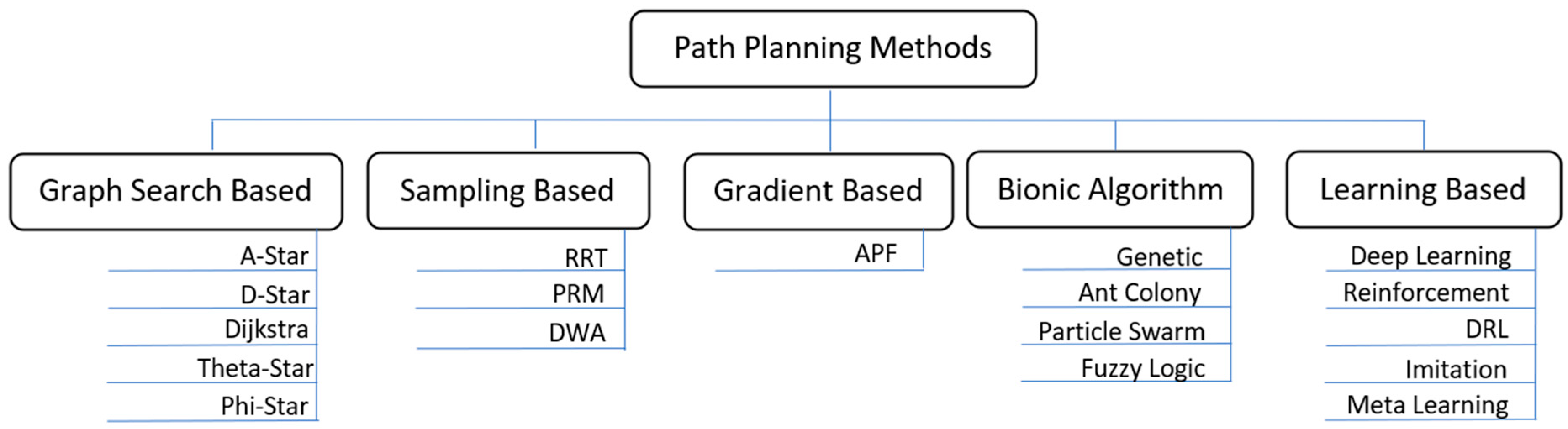
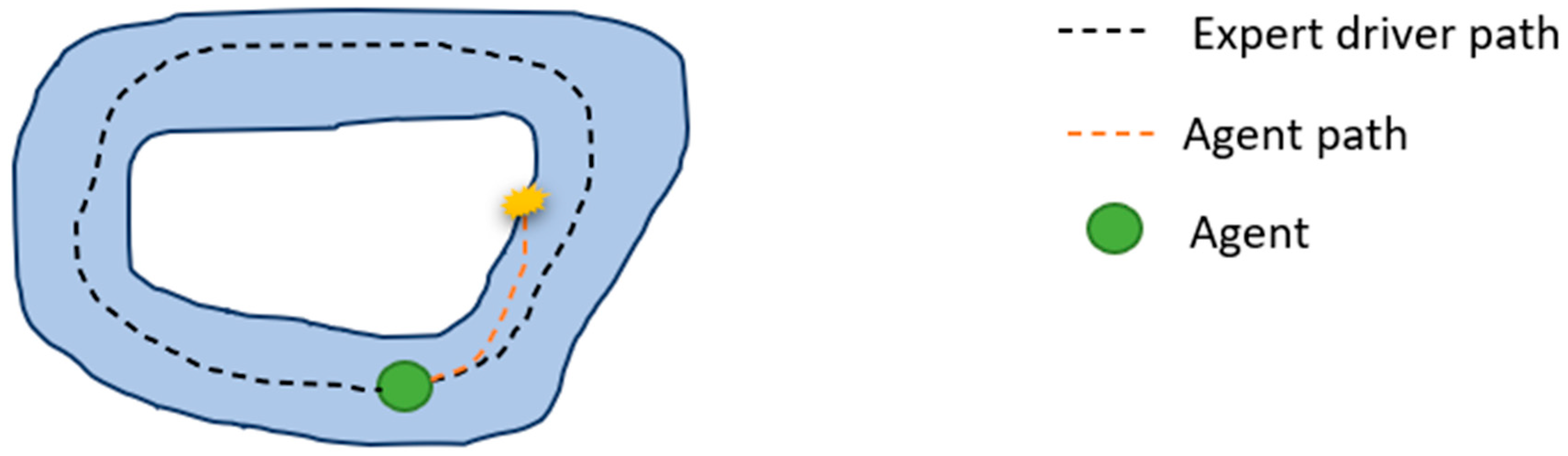
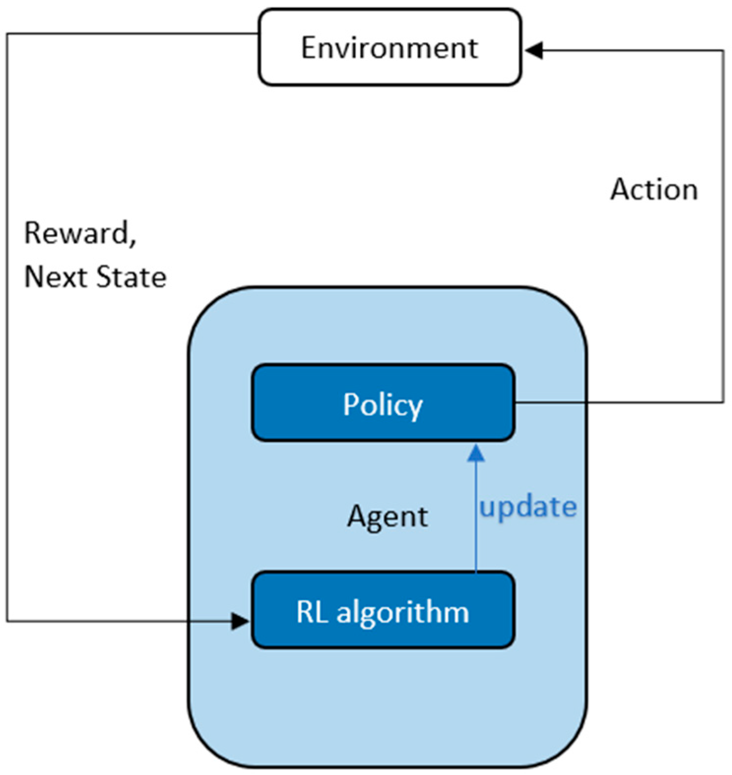
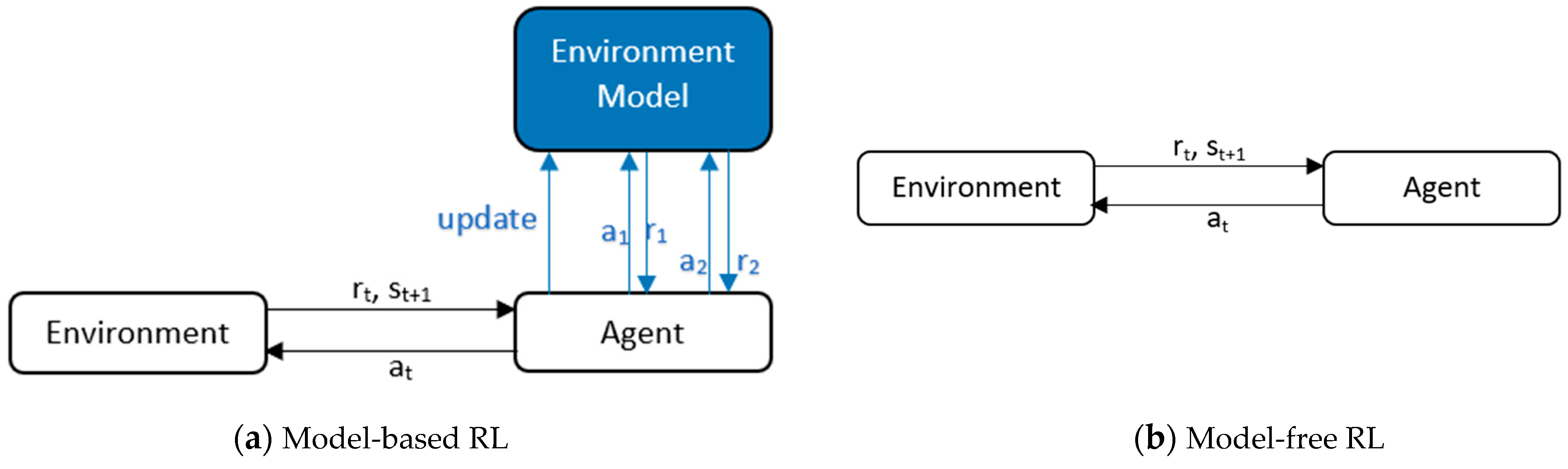
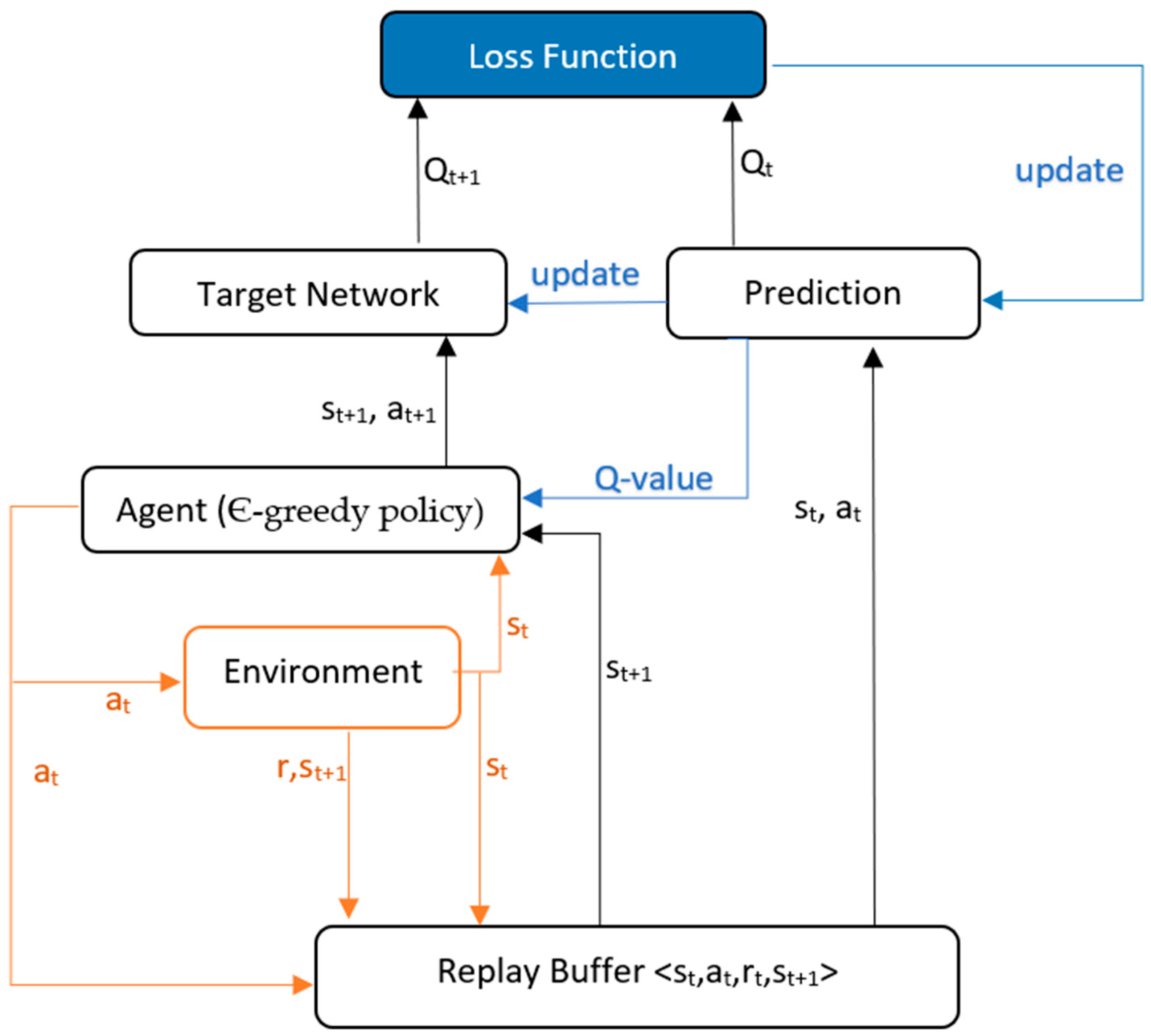
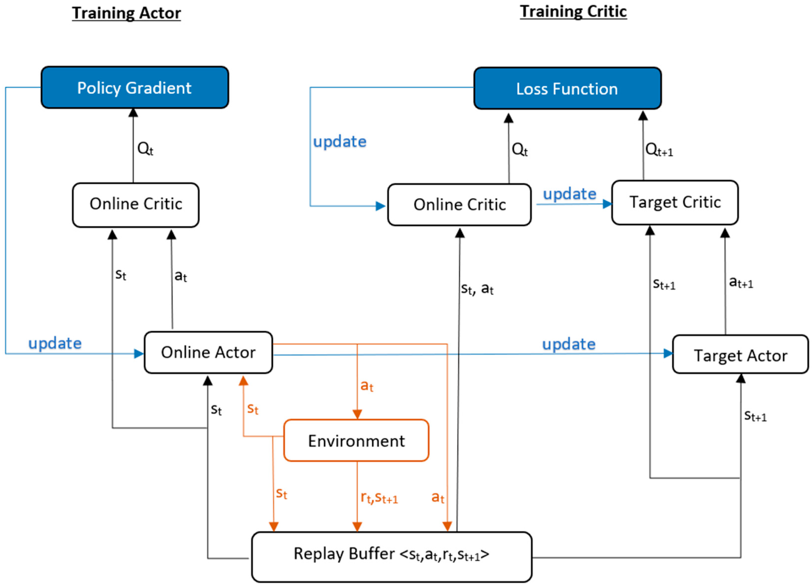
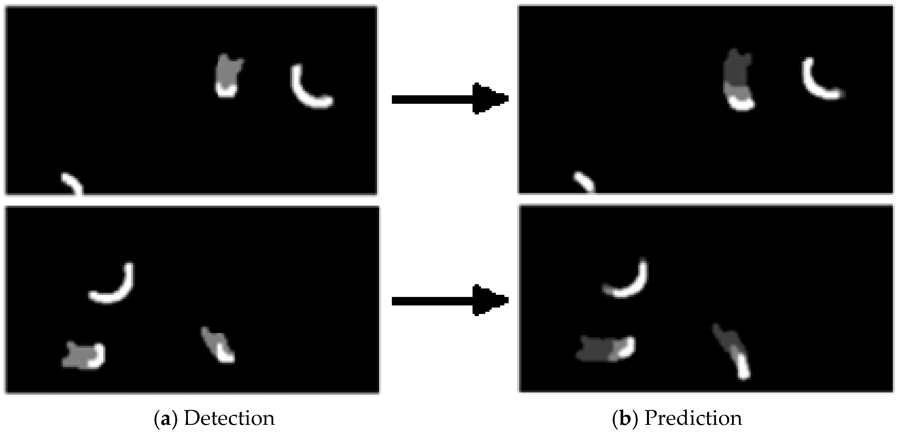
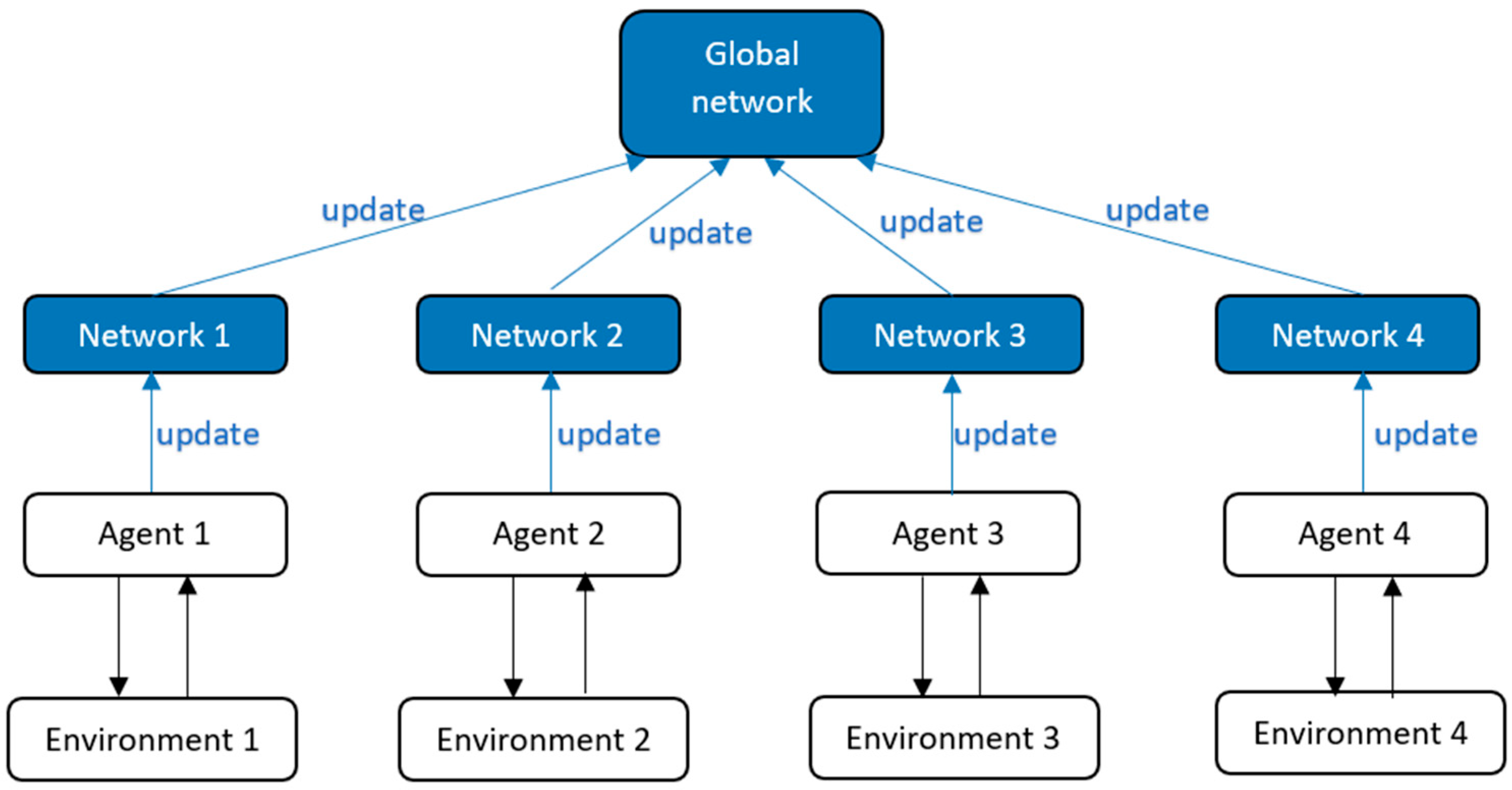
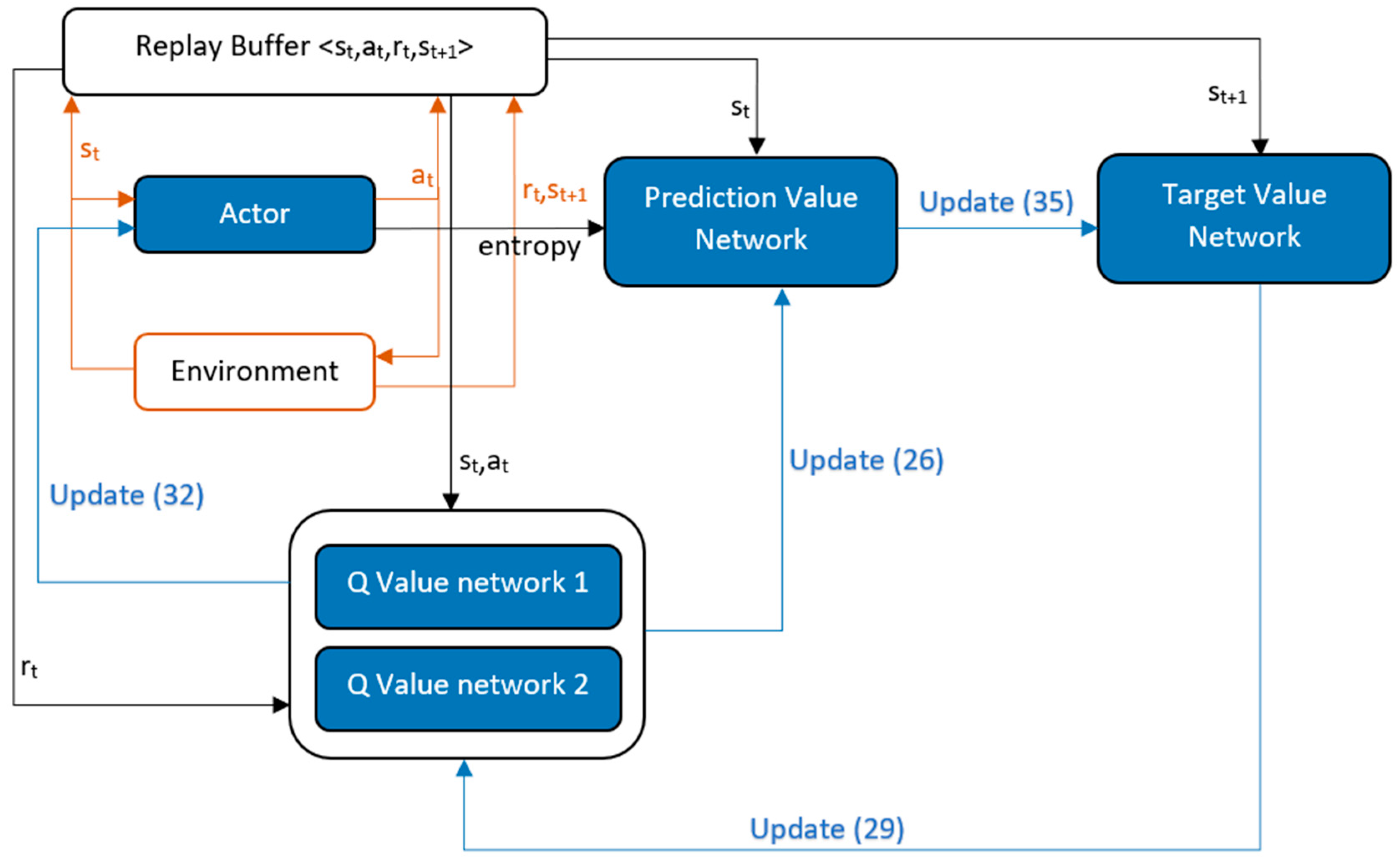
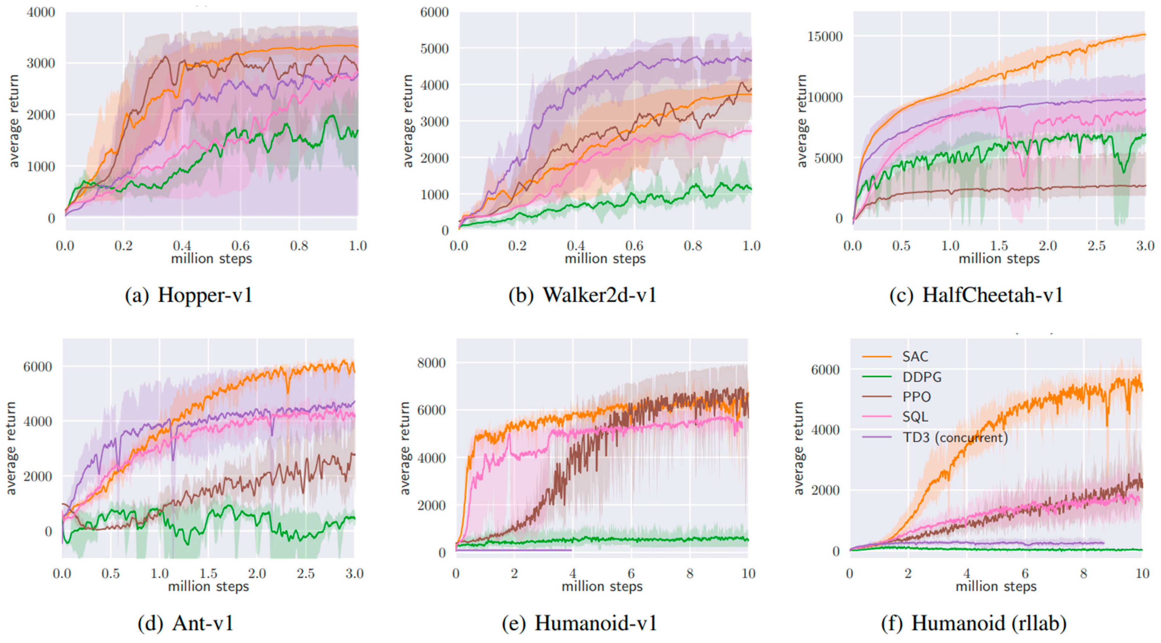
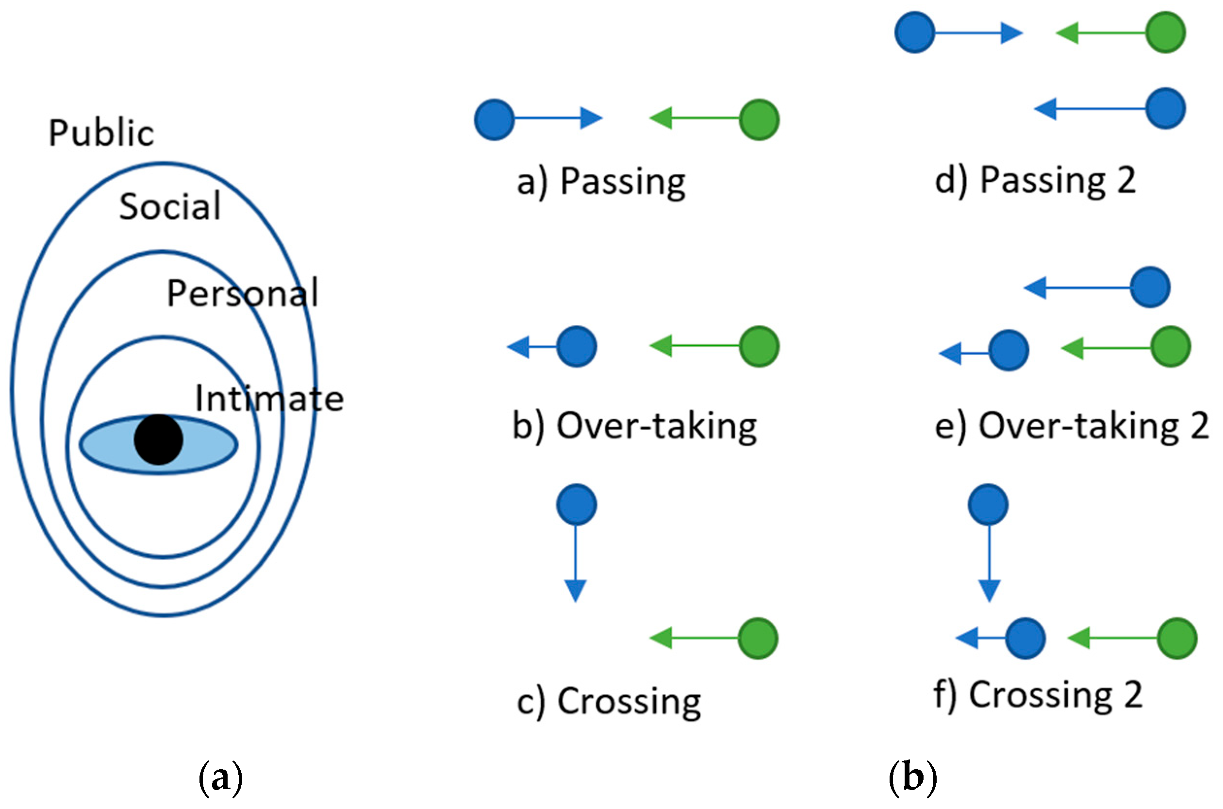
Table 1.
Summary of the DDPG method.
| Ref. | Network Input | Network Output | Training | Reward Function | Optimization | Testing | Remarks |
|---|---|---|---|---|---|---|---|
| [64] | Last 3 laser scans, Velocity, Target position | Not mentioned | Stage, Gazebo | Collision penalty, Goal reward, Change in goal relative distance reward | Proportional controller assist | Real environment with static obstacles | Trains faster, less sensitive to network structure, better than DDPG |
| [65] | 20D laser data | Angular and linear velocity | Gazebo | Collision penalty, Goal reward, change in goal relative distance reward | Curiosity module, RAdam optimizer, priority experience, transfer learning | Gazebo with dynamic obstacles | Convergence speed + 21%, success rate increased to 90% from 50% |
| [11] | 10D laser data, target position, velocity, | Angular and linear velocity | V-Rep | Collision penalty, goal reward, change in goal relative distance reward | Asynchronous training | Real environment with static obstacles | Mapless navigation capability |
| [66] | Last 10 depth images, target position | Angular and linear velocity | Gazebo | Collision penalty, goal reward, turning penalty | Real environment with dynamic obstacles | Successful navigation with dynamic obstacles | |
| [67] | 10D laser data, velocity, target position | Angular and linear velocity | Gym, Gazebo | Collision penalty, goal reward, change in goal relative distance reward | Transfer learning | Gazebo with dynamic obstacles | Performs comparable to traditional methods |
| [45] | Last 10 laser scans, velocity, target position | Angular and linear velocity | Gazebo | Collision penalty, goal reward, change in goal relative distance reward, close to static and dynamic obstacles penalty | Disentangle ego motion, Conv. LSTM layer | Real environment with dynamic obstacles | Performs better than FDMCA and MNDS [45] |
Table 2.
Summary of the A3C method.
| Ref. | Network Input | Network Output | Training | Reward Function | Optimization | Testing | Remarks |
|---|---|---|---|---|---|---|---|
| [69] | Last 3 RGB images, previous action, previous reward, agent velocity, | Rotation in small increments, accelerate forward, backward, and sideways, rotational acceleration. | Deepmind lab | Goal reward, reward in the maze to encourage exploration | Loop closure on position, RGB to depth conversion as loss function, stacked LSTM layer | Deepmind lab with static obstacles | Auxiliary tasks improve algorithm’s performance |
| [7] | Elevation map, depth image, Agent orientation, relative goal position | Forward, backward, turn left and right | Gazebo | Goal reward, change in goal relative distance reward, undesirable terminal position penalty | LSTM layer | Gazebo with static obstacles | Navigation capability in unknown environment, 80% success rate |
| [70] | Last ego-motion estimation, goal orientation, last action, last reward, Maze Map, RGB image | Forward, backward, left, right, turn left and right. | DeepMind lab | Collision penalty, goal reward, relative distance to the goal Entropy of location probability distribution | Prioritized experience replay, modular Tasks | DeepMind lab with static obstacles | Agent learns to localize on map |
| [71] | Last 4 RGB images, target image | Forward step, 90-degree turn | AI2-THOR | Goal reward, time penalty | Real environment with static obstacles | AI2-THOR renders virtual environment close to real world thus algorithm performs better in real world. | |
| [17] | Last 4 laser scans, target position | 7 discrete actions | Custom for fast parallel training | Goal reward, Collision penalty, change in goal relative distance reward, undesirable terminal position penalty | Add noise to the input | Real environment with static obstacles | Simulations run 1000 times faster than conventional methods |
| [72] | Goal distance, obstacle position and velocity, distance to obstacle | 11 discrete actions | Collision penalty, Goal reward, close to obstacle penalty | LSTM layer | Real environment with dynamic obstacles | Introduction of LSTM Layer improves performance | |
| [73] | Current state, last action, last reward | 8 discrete actions | DeepMind lab, Gazebo | Goal reward, collision penalty, change in goal relative distance reward, intrinsic reward | Intrinsic reward for exploration, stacked LSTM | Real environment with dynamic obstacles | Incorporating intrinsic Rewards doubled the extrinsic rewards collected |
Table 3.
Summary of the PPO method.
| Ref. | Network Input | Network Output | Training | Reward Function | Optimization | Testing | Remarks |
|---|---|---|---|---|---|---|---|
| [76] | Greyscale height map, target position, robot pose | Move in the x- and y-axis, Rotate, change height, change width | V-Rep | Collision penalty, time penalty, change in goal relative distance reward | Domain randomization | V-Rep with static obstacles | Use of domain randomized trajectory improves the output. |
| [77] | Surrounding 8 tiles, nearest uncleaned tile | Move forward, Turn 45 degree | Python GUI Tkinter | Cleaned tile penalty, wall collision penalty, rotation penalty, intrinsic reward | Intrinsic reward Transfer learning Elite set | Python GUI Tkinter | Navigation performed on a grid-based environment |
| [78] | Last 4 depth images, Last 3 laser scans, target position, velocity | 10 discrete actions | Gazebo | Collision penalty, goal reward, change in goal relative distance reward, slip rate/angle penalty | Gazebo with static obstacles | Cannot reach target when target is very far or there are very large craters. | |
| [80] | 4 checkpoints, velocity, 12D laser data, | Linear and angular velocity | Unity | Checkpoint reward, time penalty, collision penalty, | Unity with static obstacles, maze-like maps | Algorithm sometimes jump checkpoints to give efficient paths. | |
| [18] | Last 3 depth images, Last 3 laser scans, target position, velocity | Linear and angular velocity | Gazebo | Collision penalty, goal reward, change in goal relative distance reward, Close to obstacle penalty, angular velocity penalty, waypoint reward | Transfer learning | Real-world with dynamic obstacles | Susceptible to robot freezing in very dense environment, works well in complex, occluded scenarios and results in smoother trajectories |
| [8] | Laser scans | 8 discrete actions | Custom | Collision penalty, goal reward, timestep penalty | Real-world with static obstacles. | Number of training epochs is much less compared to other methods |
Table 4.
Summary of the SAC method.
| Ref. | Network Input | Network Output | Training | Reward Function | Optimization | Testing | Remarks |
|---|---|---|---|---|---|---|---|
| [82] | Location and velocity of agent and obstacles, target location | Linear and angular velocity | Pygame | Face toward the target, move toward the target, close to obstacle penalty, terminal state reward | Prioritized experience replay, state action normalization | Pygame with dynamic obstacles | Performs better than PPO, tested in only 1 2D environment |
| [83] | Last 2 horizontal depth image planes and their difference, target position, last action | Linear and angular velocity | Gazebo | Goal reward, collision penalty, going toward goal reward, going away from goal penalty | Transfer learning | Real environment with dynamic obstacles | Maximum success rate is 47% |
| [84] | Last 3 laser scans, velocity, target position | Linear and angular velocity | Gazebo | Goal reward, collision penalty, going toward goal reward, rotation velocity penalty | Real environment with dynamic obstacles | Performed well in dynamic environment, unable to efficiently move in straight line. Might solve with more training in that environment. | |
| [85] | LiDAR data, 6 waypoints, target position | Linear and angular velocity | Gibson | Goal reward, collision penalty, going toward waypoint reward, reaching waypoint reward, timestep penalty | Transfer learning | Gibson with dynamic obstacles | The learned policy demonstrates behaviors such as slowing down, navigating around pedestrians, and reversing to manage various interactions. |
Disclaimer/Publisher’s Note: The statements, opinions and data contained in all publications are solely those of the individual author(s) and contributor(s) and not of MDPI and/or the editor(s). MDPI and/or the editor(s) disclaim responsibility for any injury to people or property resulting from any ideas, methods, instructions or products referred to in the content. |
© 2023 by the authors. Licensee MDPI, Basel, Switzerland. This article is an open access article distributed under the terms and conditions of the Creative Commons Attribution (CC BY) license (https://creativecommons.org/licenses/by/4.0/).
Share and Cite
MDPI and ACS Style
Singh, R.; Ren, J.; Lin, X. A Review of Deep Reinforcement Learning Algorithms for Mobile Robot Path Planning. Vehicles 2023, 5, 1423-1451. https://doi.org/10.3390/vehicles5040078
AMA Style
Singh R, Ren J, Lin X. A Review of Deep Reinforcement Learning Algorithms for Mobile Robot Path Planning. Vehicles. 2023; 5(4):1423-1451. https://doi.org/10.3390/vehicles5040078
Chicago/Turabian StyleSingh, Ramanjeet, Jing Ren, and Xianke Lin. 2023. "A Review of Deep Reinforcement Learning Algorithms for Mobile Robot Path Planning" Vehicles 5, no. 4: 1423-1451. https://doi.org/10.3390/vehicles5040078