Author Contributions
Conceptualisation, K.S. and D.R.; methodology, K.S., D.L. and I.G.; software, K.S.; validation, K.S.; formal analysis, D.R.; investigation, K.S.; resources, K.S.; data curation, K.S.; writing—original draft preparation, K.S.; writing—review and editing, D.R., I.G. and P.K.; visualisation, K.S.; supervision, D.L, I.G., P.K. and D.R.; project administration, K.S., D.L. and D.R. All authors have read and agreed to the published version of the manuscript.
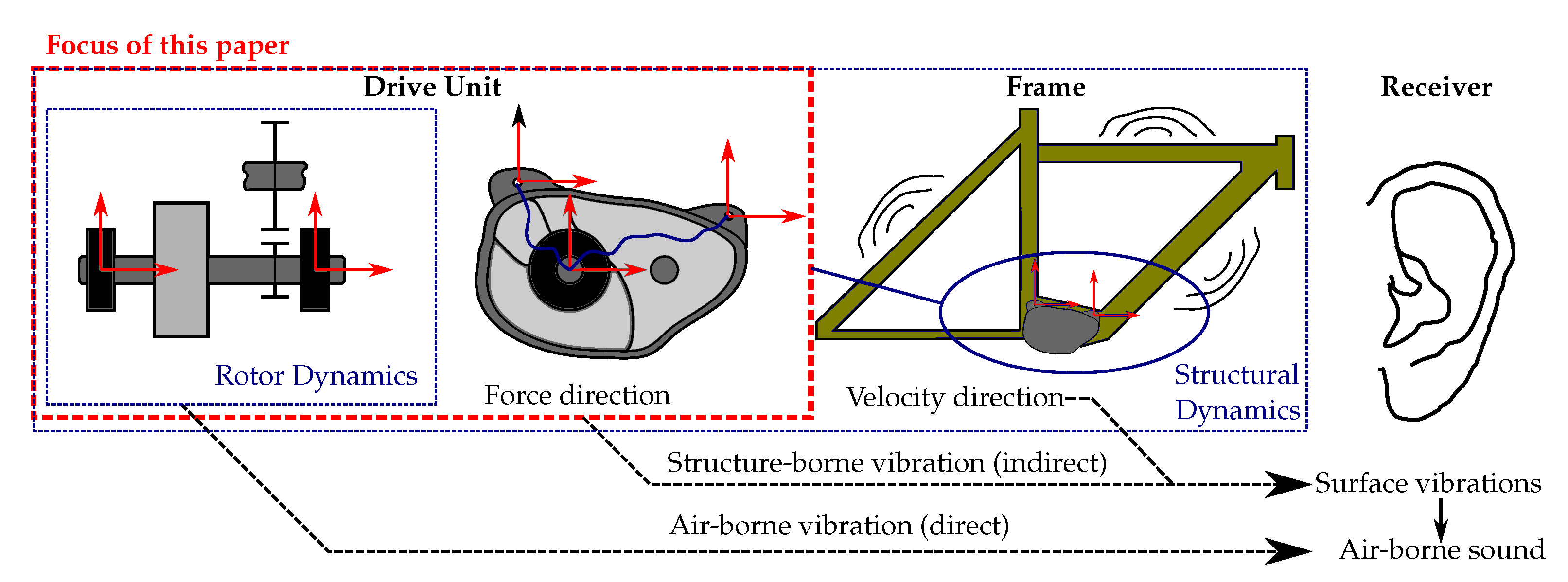
Figure 1.
Schematic sound transmission transfer path.
Figure 1.
Schematic sound transmission transfer path.
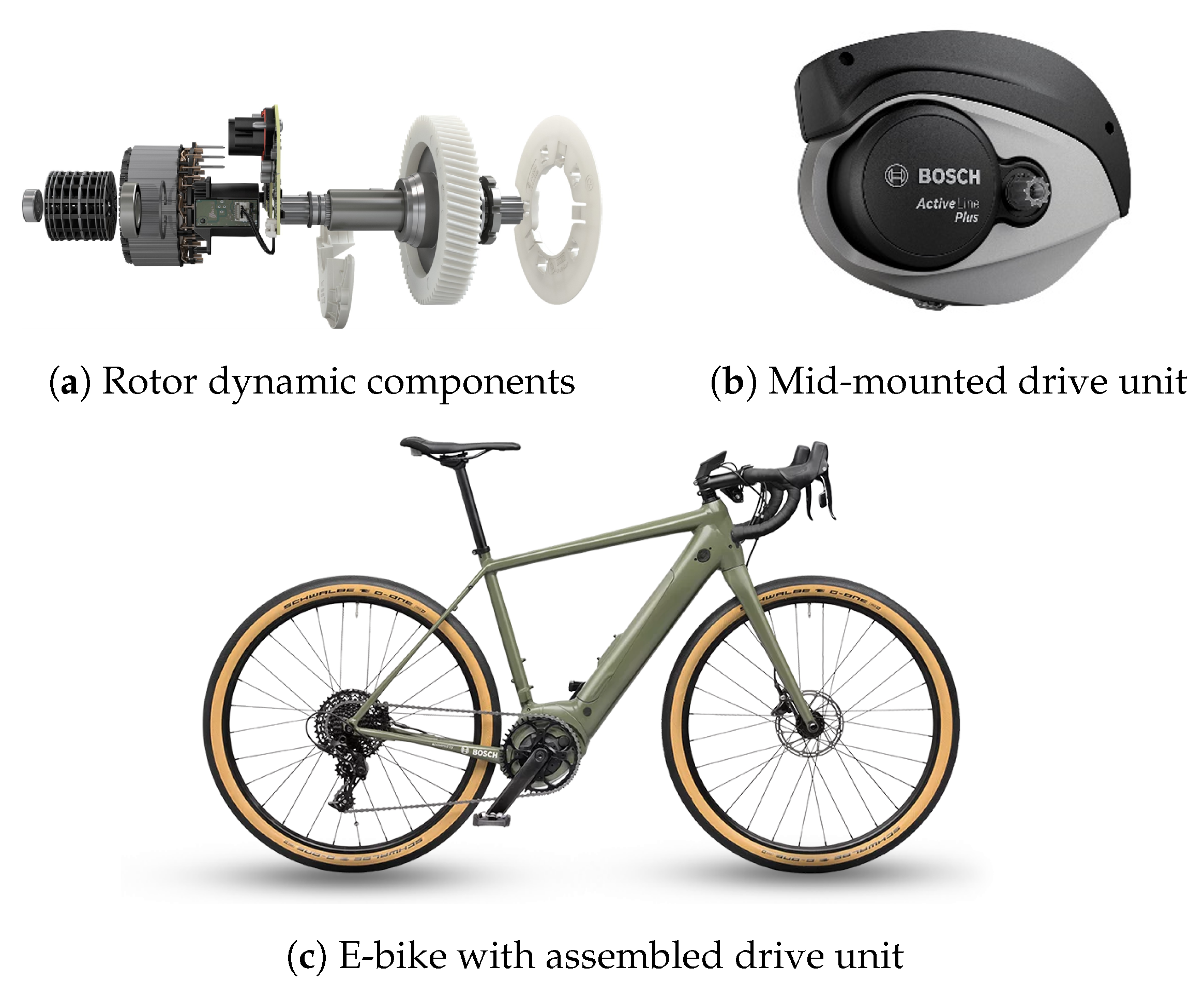
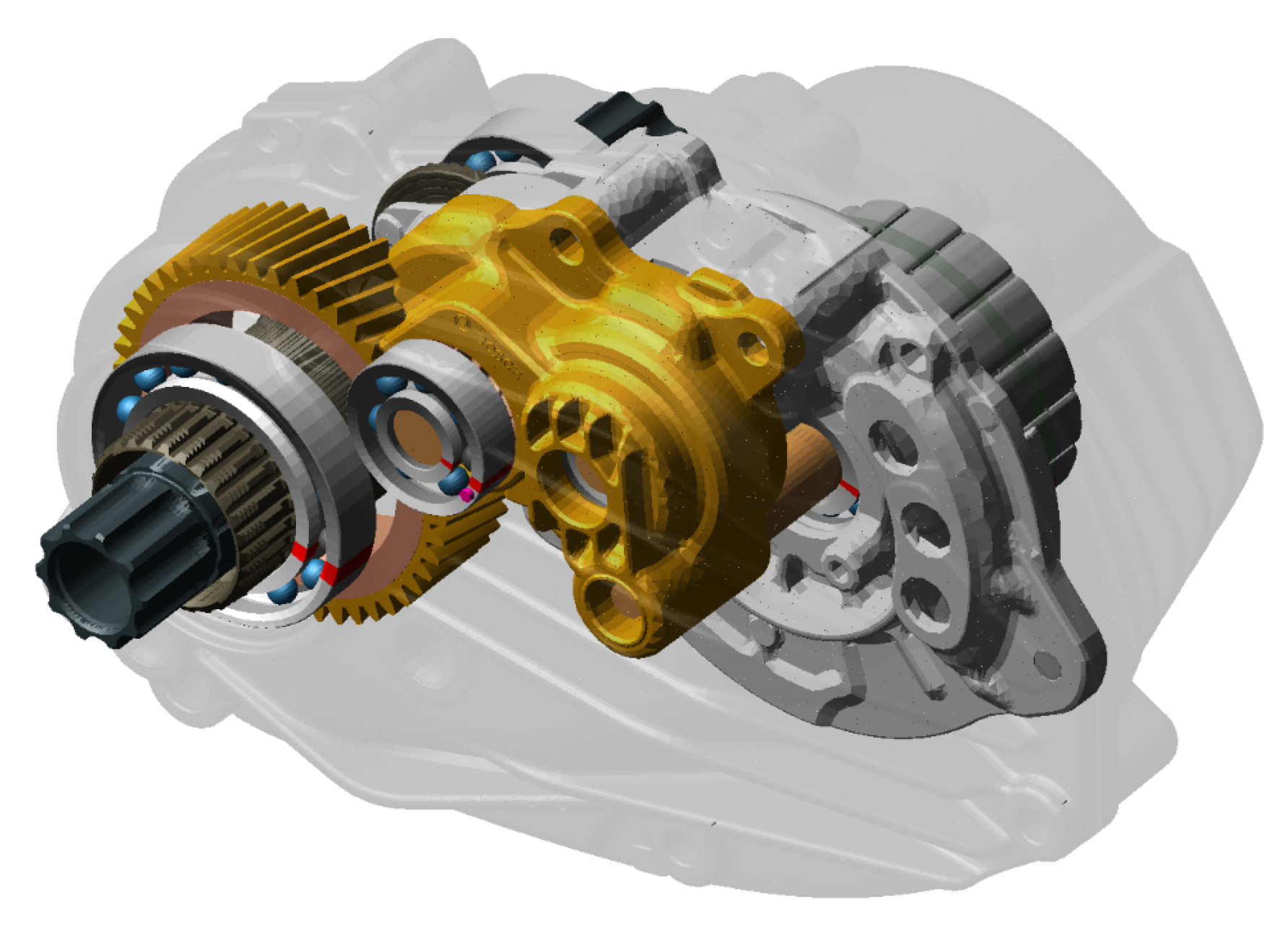
Figure 2.
Example of a mid-mounted Bosch drive unit and their assembly in an e-bike [
24].
Figure 2.
Example of a mid-mounted Bosch drive unit and their assembly in an e-bike [
24].
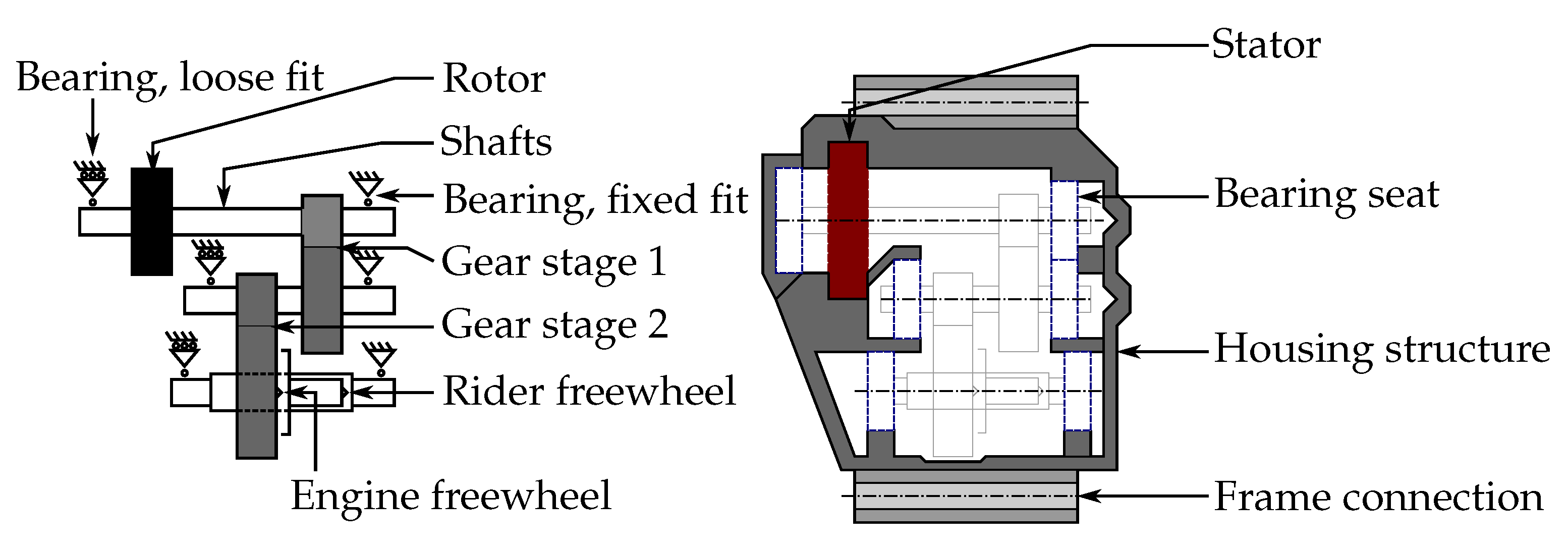
Figure 3.
Schematic illustration of the drive unit’s rotating parts with the intersection at the bearing seat (left) and the surrounding housing structure (right).
Figure 3.
Schematic illustration of the drive unit’s rotating parts with the intersection at the bearing seat (left) and the surrounding housing structure (right).
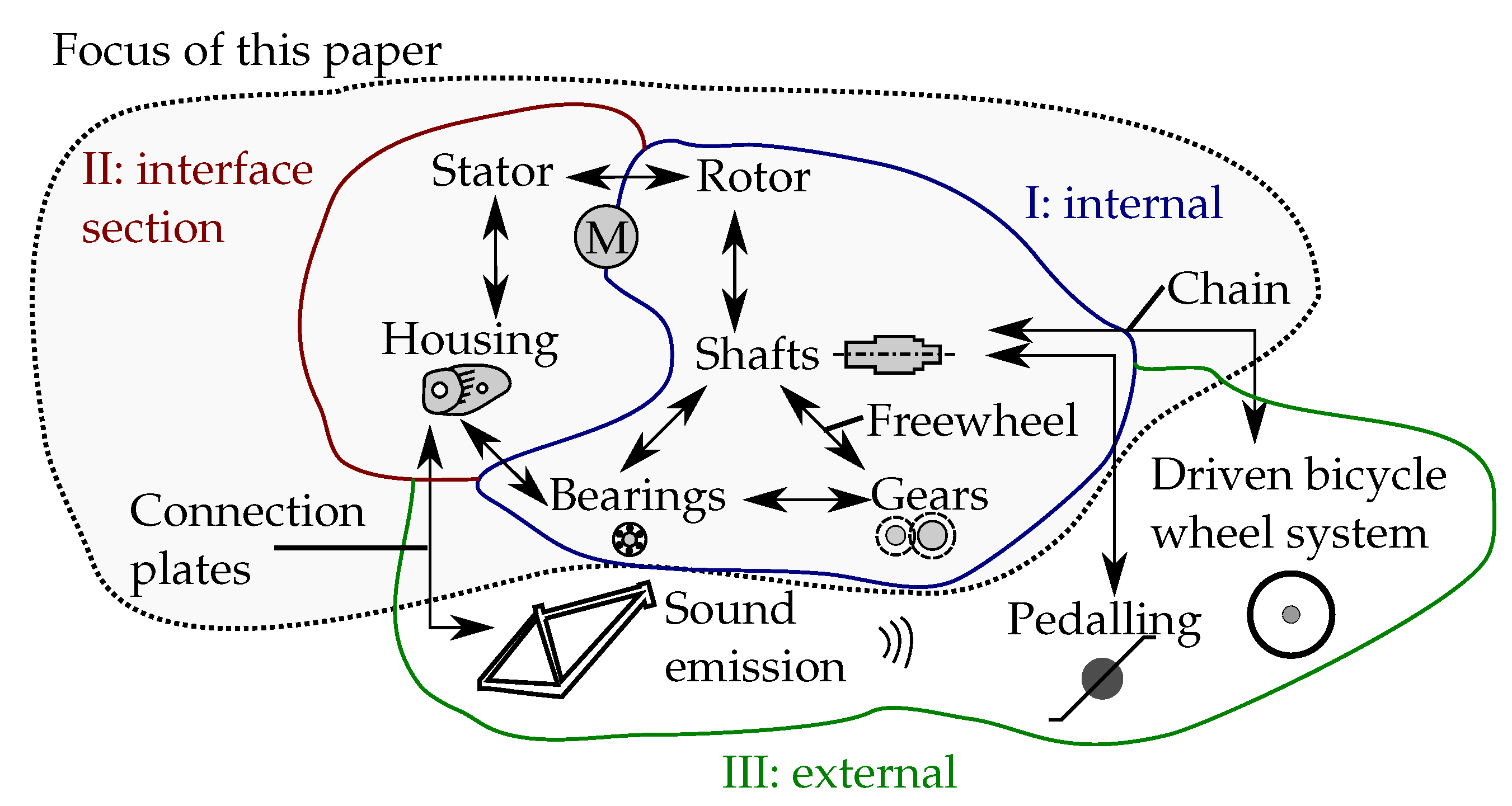
Figure 4.
Structural dynamic interactions of the e-bike drive unit. The arrows show the force flow. I: rotor dynamics; II: drive unit structure; III: surrounding bicycle structure.
Figure 4.
Structural dynamic interactions of the e-bike drive unit. The arrows show the force flow. I: rotor dynamics; II: drive unit structure; III: surrounding bicycle structure.
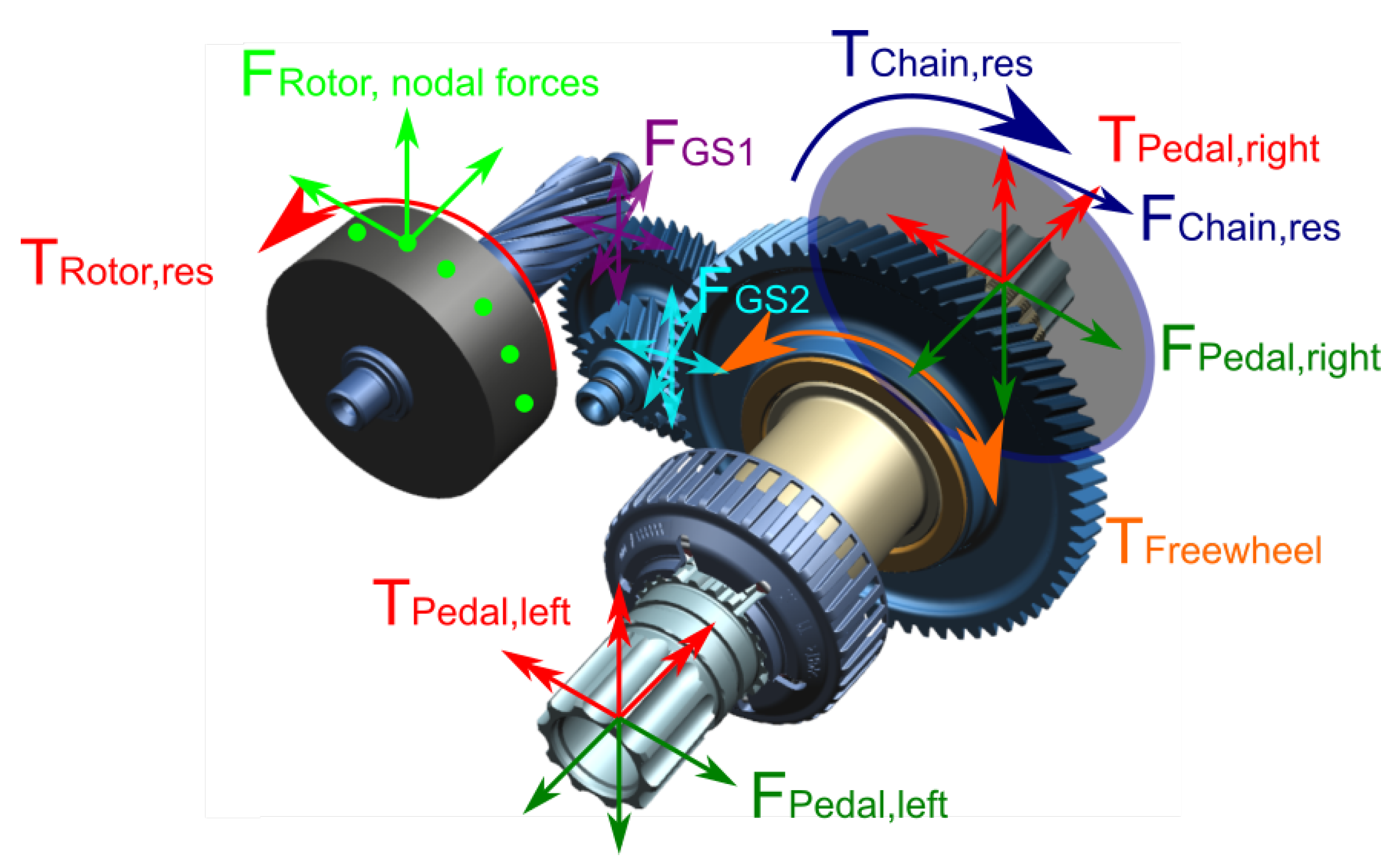
Figure 5.
Excitation illustrated by forces and torques acting on the rotor dynamic parts. For clarity, both the bearing as well as the stator reaction forces are not illustrated.
Figure 5.
Excitation illustrated by forces and torques acting on the rotor dynamic parts. For clarity, both the bearing as well as the stator reaction forces are not illustrated.
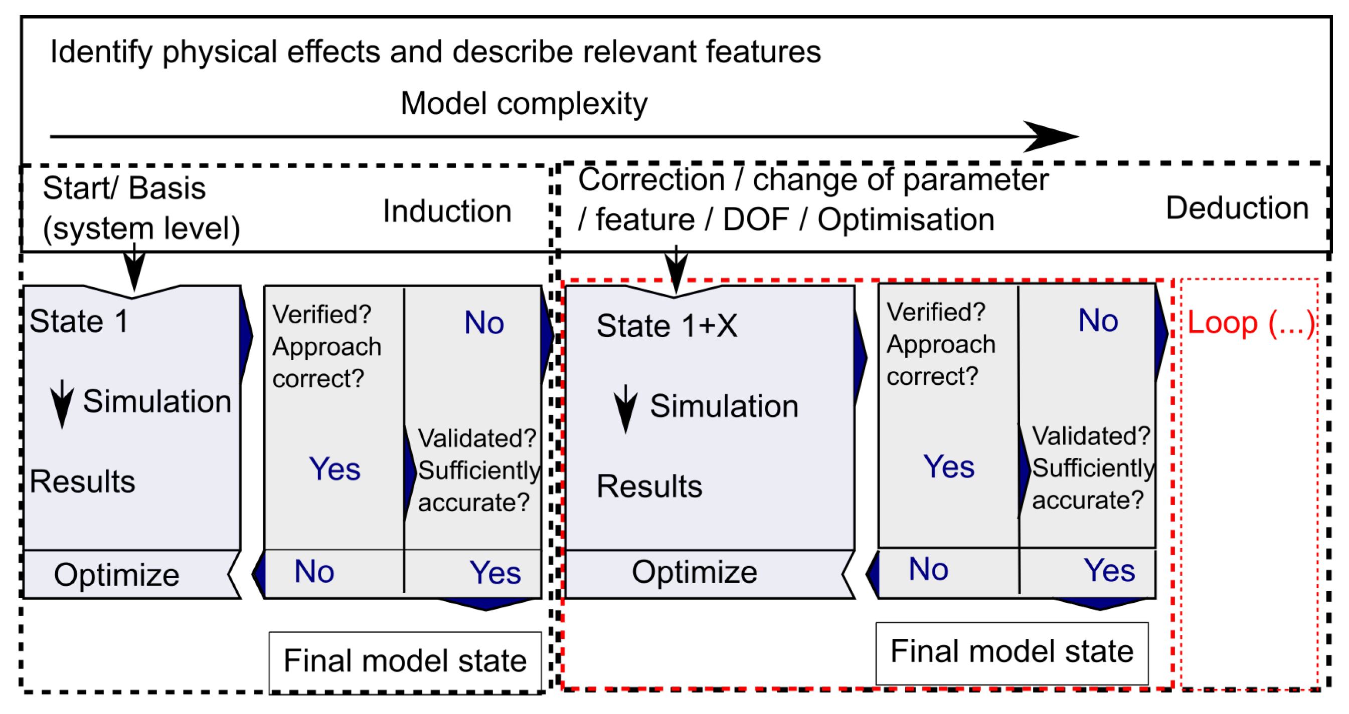
Figure 6.
Evolved method based on induction and deduction for the model development process.
Figure 6.
Evolved method based on induction and deduction for the model development process.
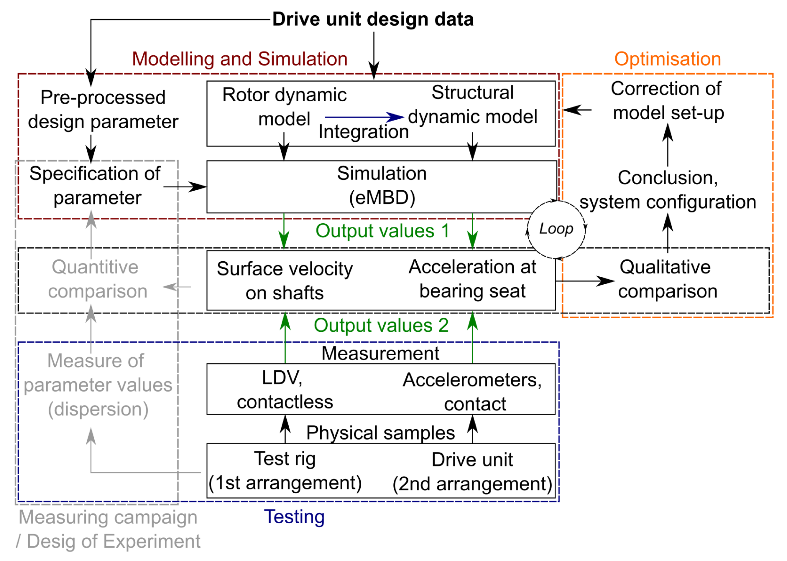
Figure 7.
Overall method for model development and validation including simulation and testing. The loop indicates the further processing and the grey coloured subjects are neglected.
Figure 7.
Overall method for model development and validation including simulation and testing. The loop indicates the further processing and the grey coloured subjects are neglected.
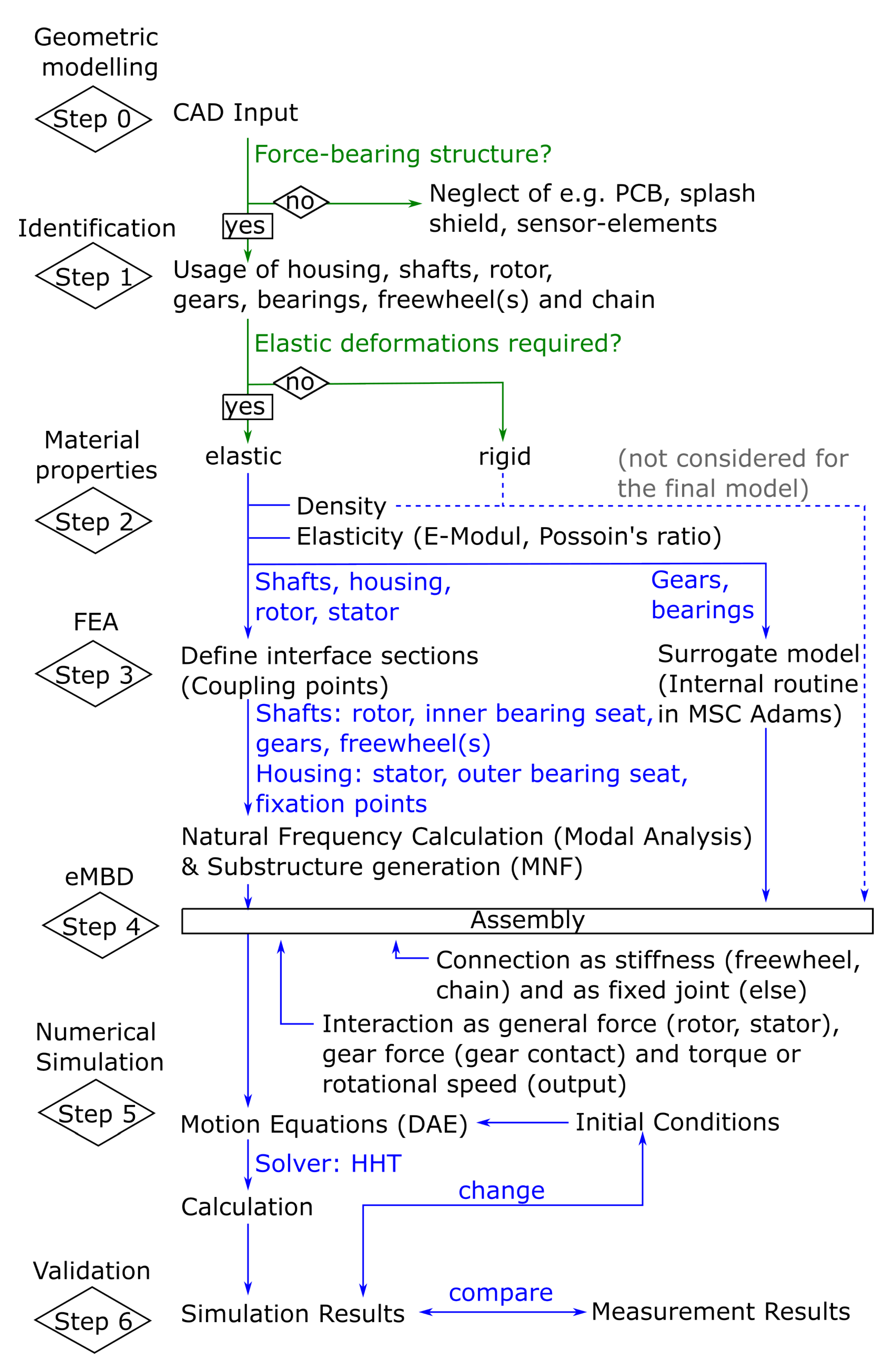
Figure 8.
Methodology to establish the eMBD system model.
Figure 8.
Methodology to establish the eMBD system model.
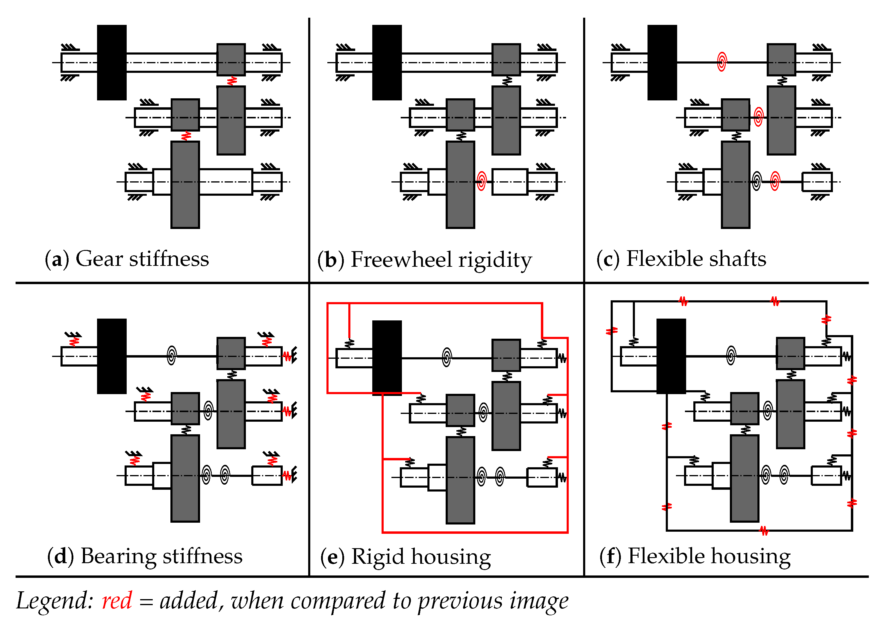
Figure 9.
Schematic sub-model identification. Steps (a–f) show the changed parameters.
Figure 9.
Schematic sub-model identification. Steps (a–f) show the changed parameters.
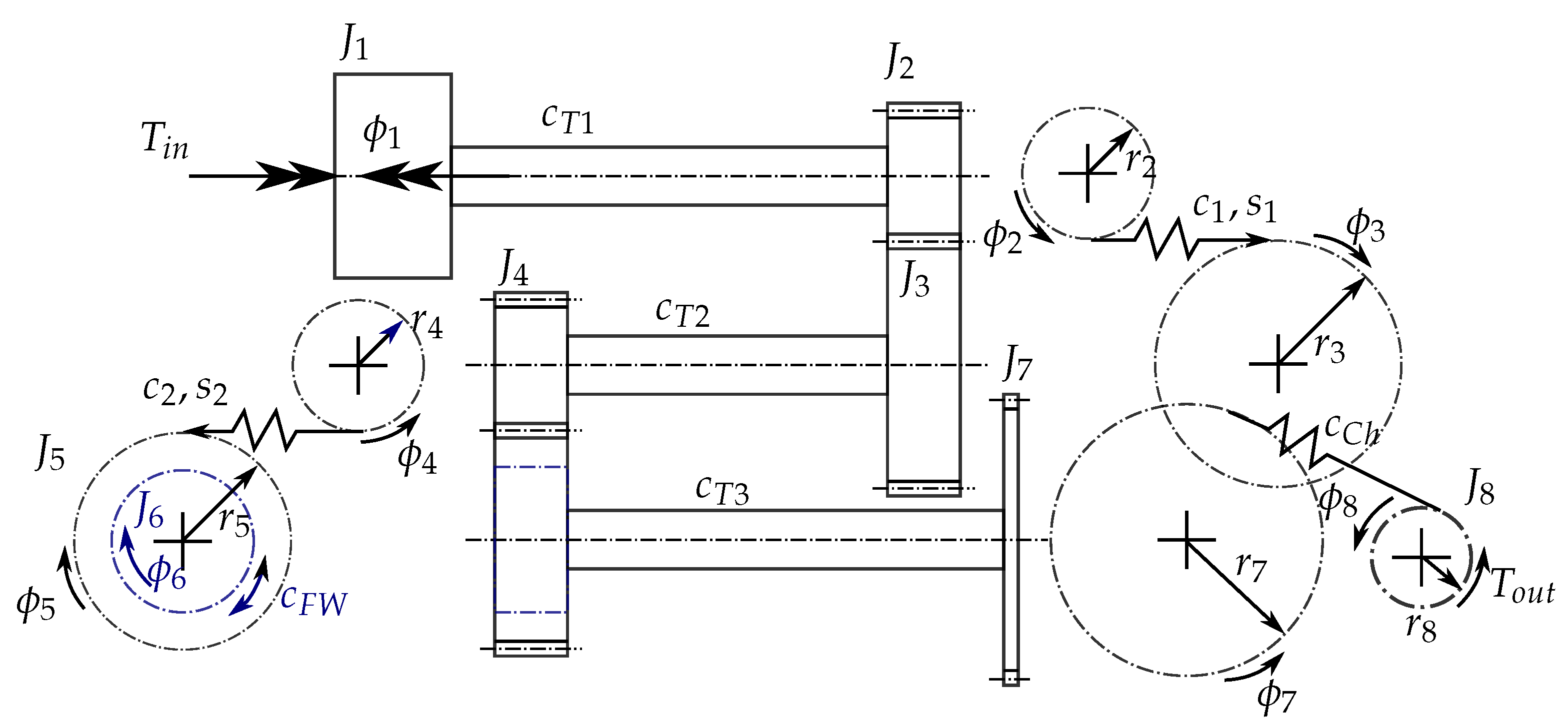
Figure 10.
A torsional oscillator system model of the e-bike drive unit with two gear stages considering rotor, shafts, gears, freewheel, chain and applied torque.
Figure 10.
A torsional oscillator system model of the e-bike drive unit with two gear stages considering rotor, shafts, gears, freewheel, chain and applied torque.
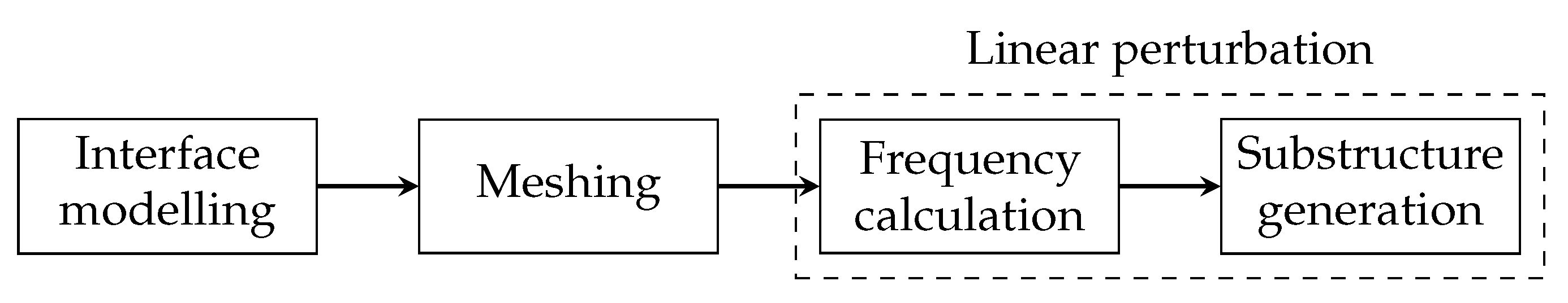
Figure 11.
The principle steps of the FEM pre-processing.
Figure 11.
The principle steps of the FEM pre-processing.
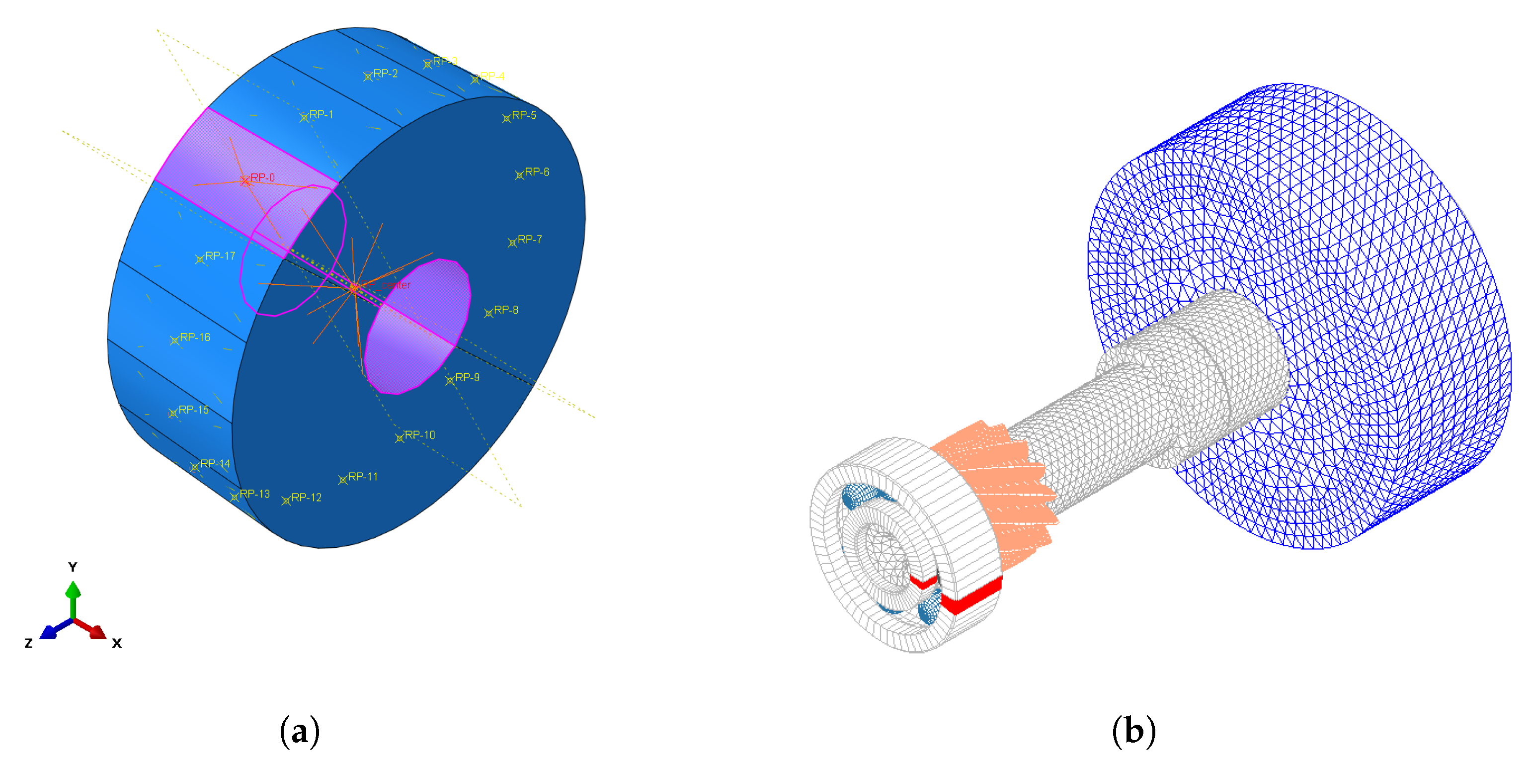
Figure 12.
Example illustration of the used interface modelling. (a) Coupling constraints of the rotor within the FEM. (b) Rotor linked with further components within the eMBD model later on.
Figure 12.
Example illustration of the used interface modelling. (a) Coupling constraints of the rotor within the FEM. (b) Rotor linked with further components within the eMBD model later on.
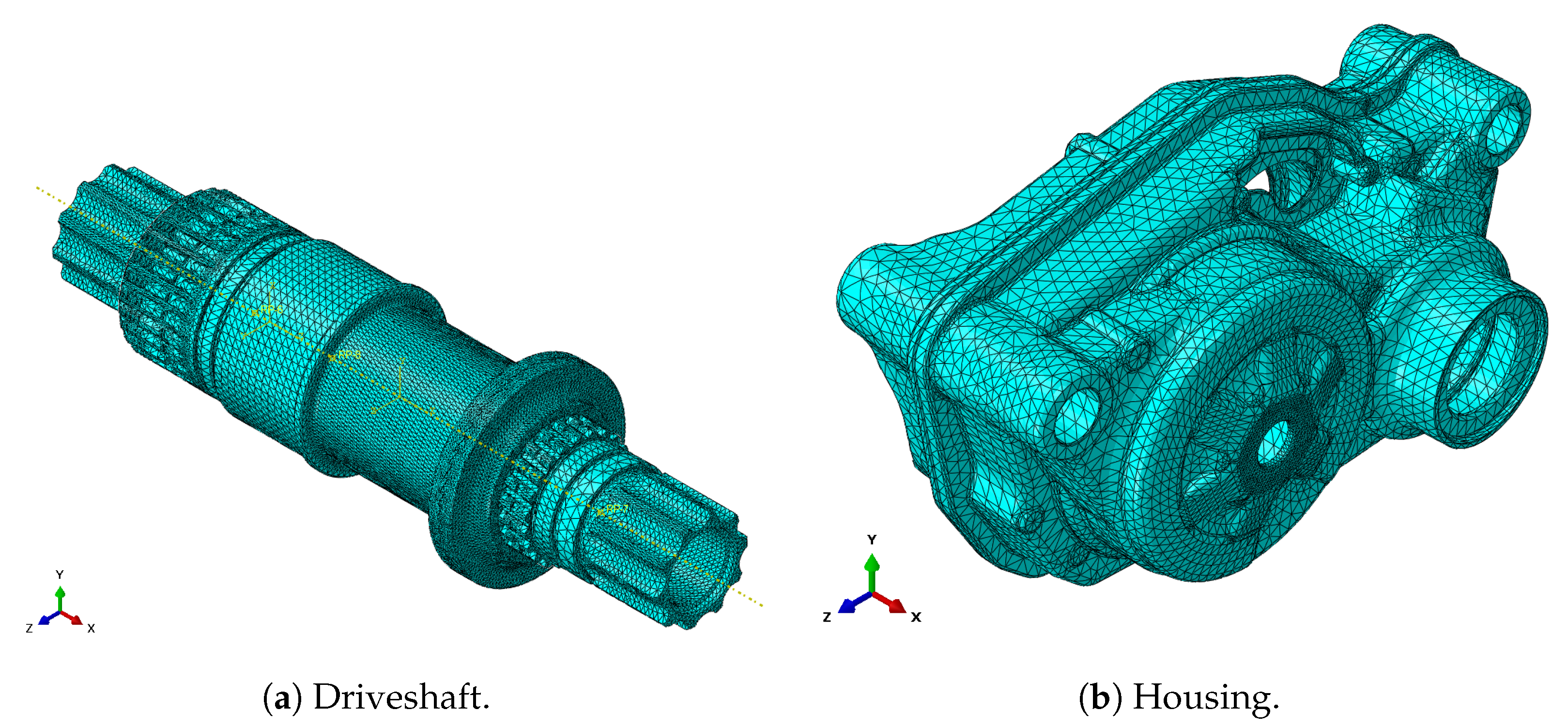
Figure 13.
Example of meshed components with quadratic tetrahedral elements.
Figure 13.
Example of meshed components with quadratic tetrahedral elements.
Figure 14.
Example of Bosch Performance Line CX as elastic multi-body-dynamic model in MSC Adams created by the introduced method.
Figure 14.
Example of Bosch Performance Line CX as elastic multi-body-dynamic model in MSC Adams created by the introduced method.
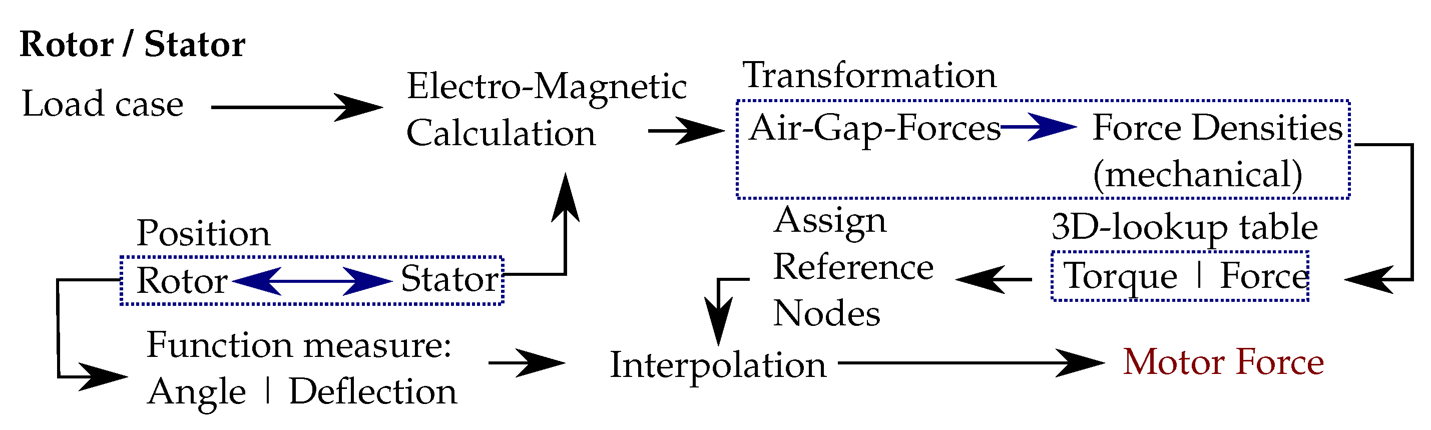
Figure 15.
Rotor and stator forces are looked up.
Figure 15.
Rotor and stator forces are looked up.
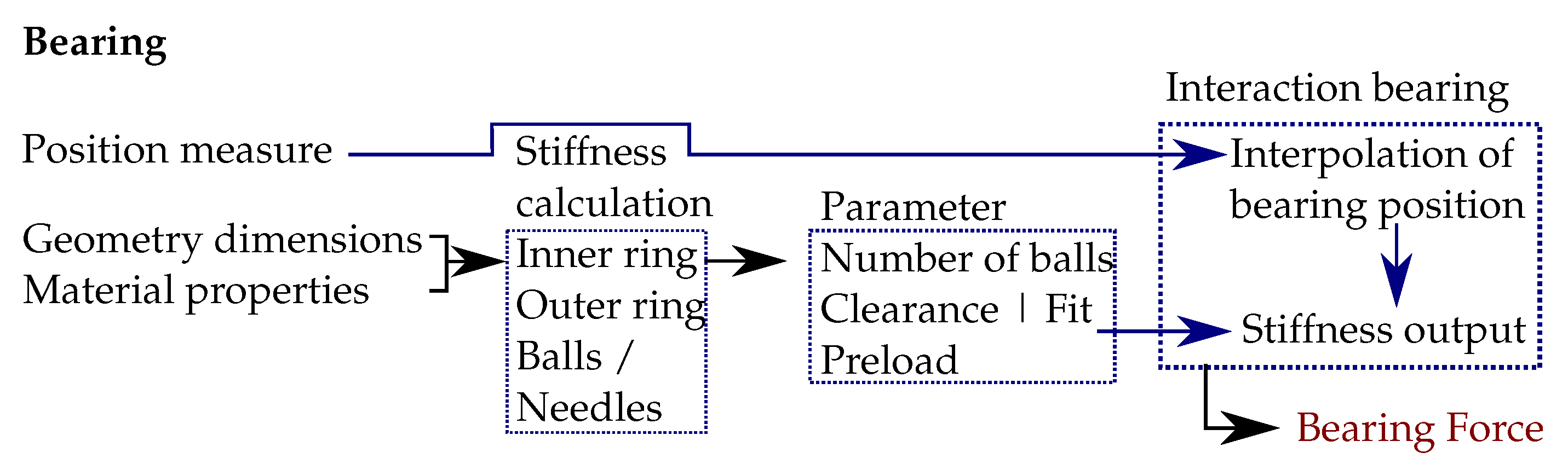
Figure 16.
Implementation of the bearing stiffness.
Figure 16.
Implementation of the bearing stiffness.
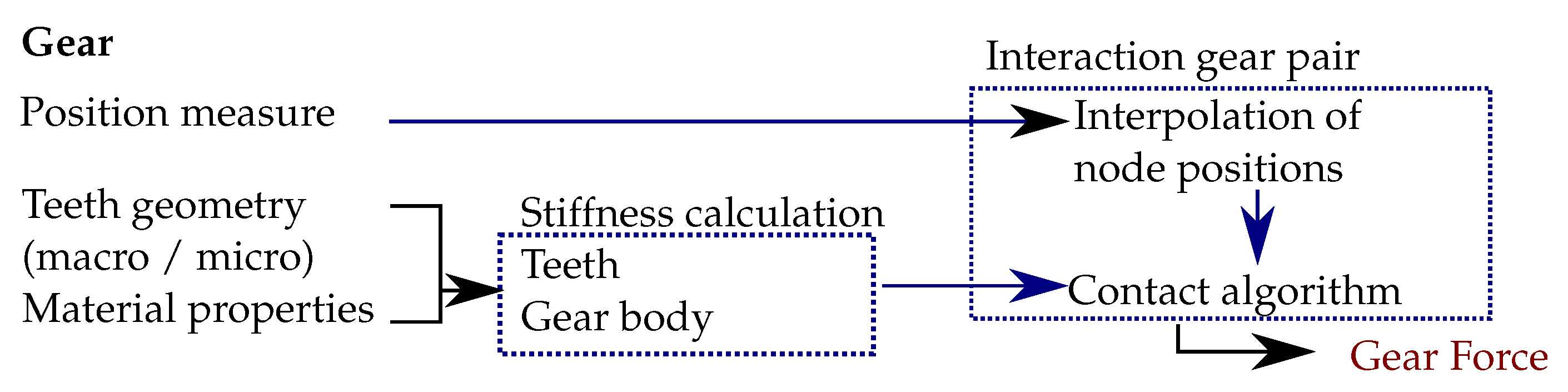
Figure 17.
Implementation of the gear stiffness.
Figure 17.
Implementation of the gear stiffness.
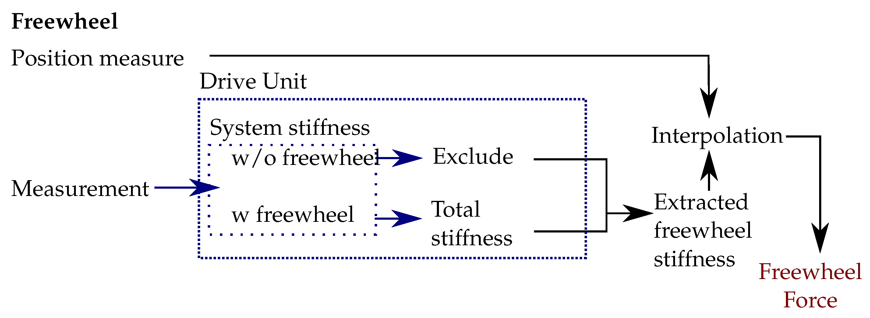
Figure 18.
Processing and implementation of the measured freewheel stiffness.
Figure 18.
Processing and implementation of the measured freewheel stiffness.
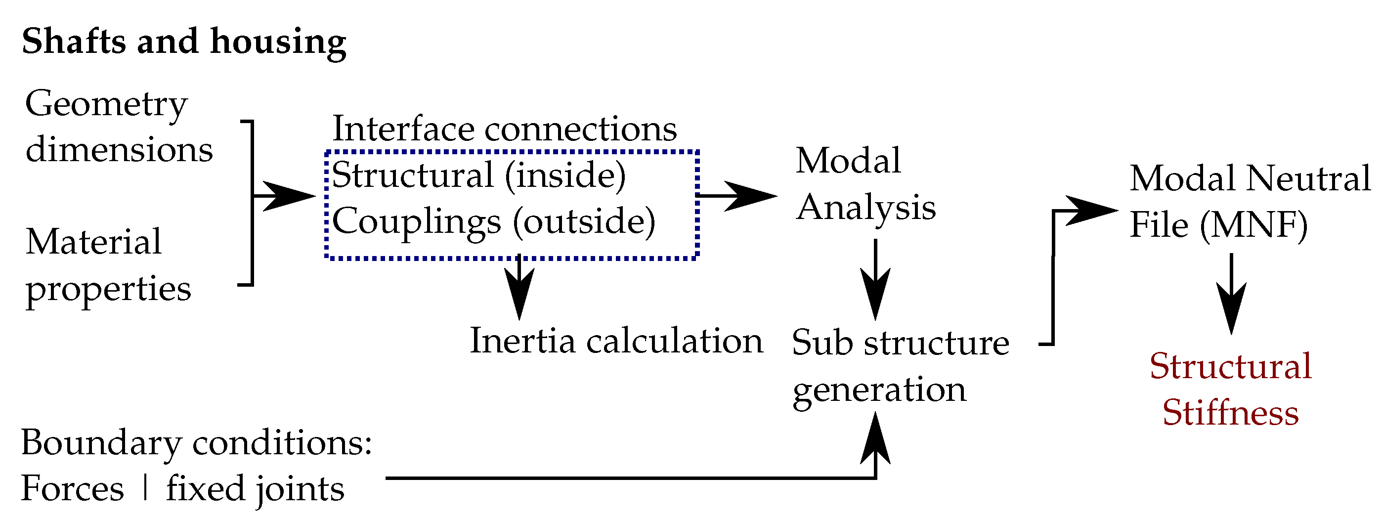
Figure 19.
Pre-processing and implementation of the structural parts, like shafts and housing.
Figure 19.
Pre-processing and implementation of the structural parts, like shafts and housing.
Figure 20.
The principle steps to validate the simulation model.
Figure 20.
The principle steps to validate the simulation model.
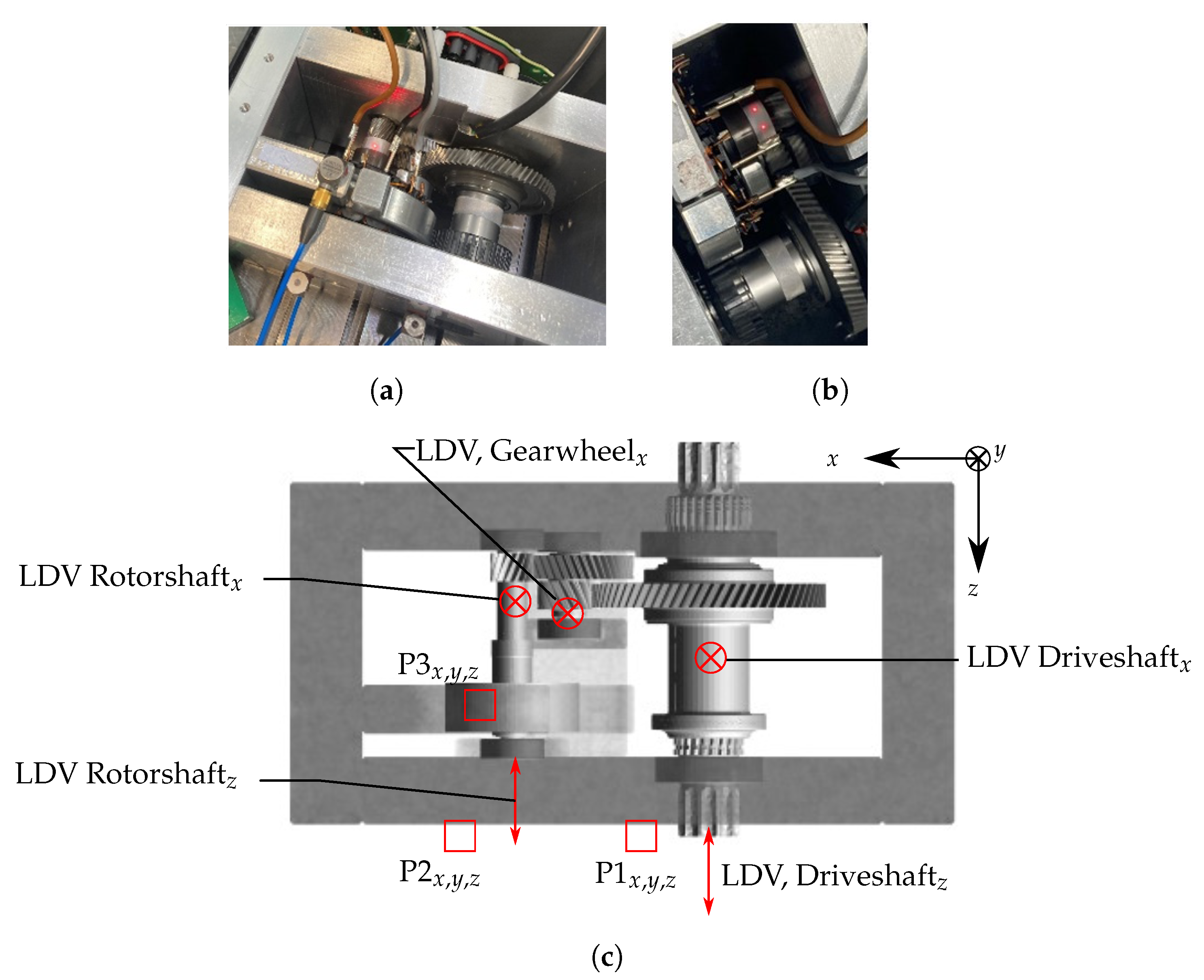
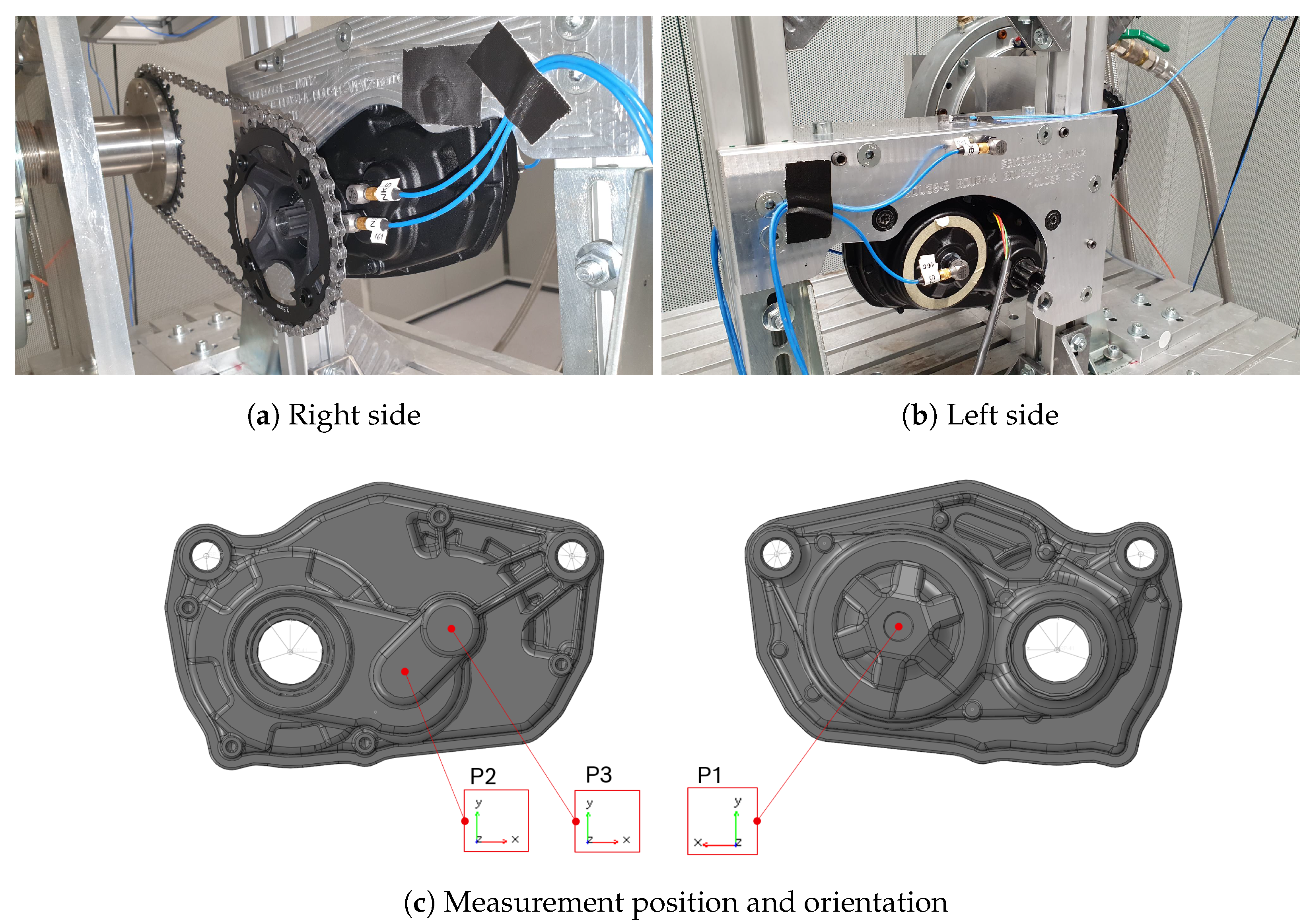
Figure 21.
Test rig arrangement of both the simulation model and the physical measurement. (a) Exemplary radial LDV measurement. (b) Exemplary rotational LDV measurement. (c) Simulation model and illustration of the positions to evaluate the motion variables.
Figure 21.
Test rig arrangement of both the simulation model and the physical measurement. (a) Exemplary radial LDV measurement. (b) Exemplary rotational LDV measurement. (c) Simulation model and illustration of the positions to evaluate the motion variables.
Figure 22.
Measurement of the Bosch Drive Unit with accelerometers close to the bearing seat.
Figure 22.
Measurement of the Bosch Drive Unit with accelerometers close to the bearing seat.
Figure 23.
Model variation and simulation for verification purposes. Each step of making the model more complex shows which further information is in the model.
Figure 23.
Model variation and simulation for verification purposes. Each step of making the model more complex shows which further information is in the model.
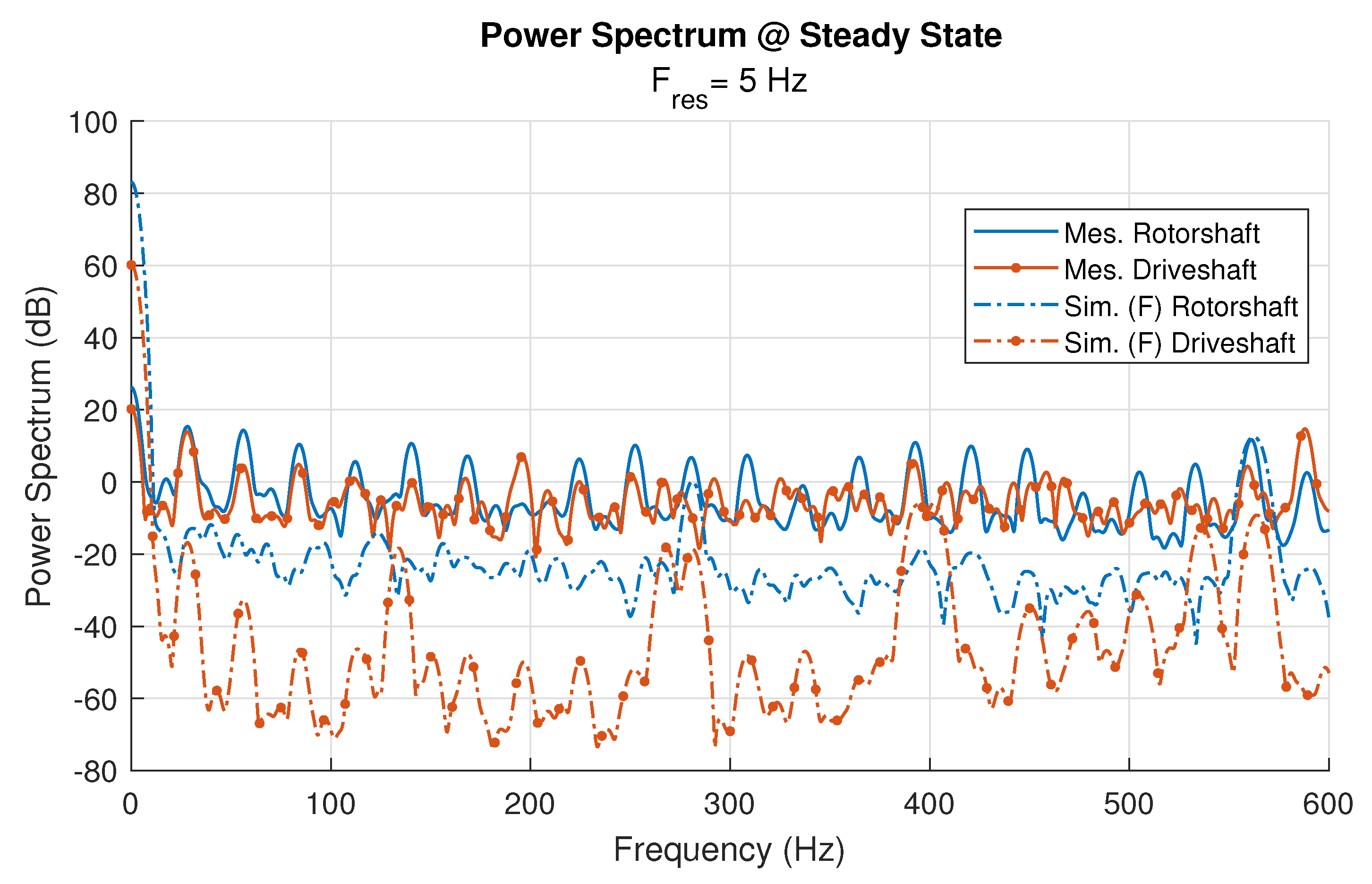
Figure 24.
Comparison with the measurement result of the rotorshaft and driveshaft rotational oscillations. The dash lines show the simulation results, and the colours, the affiliation with the measurements.
Figure 24.
Comparison with the measurement result of the rotorshaft and driveshaft rotational oscillations. The dash lines show the simulation results, and the colours, the affiliation with the measurements.
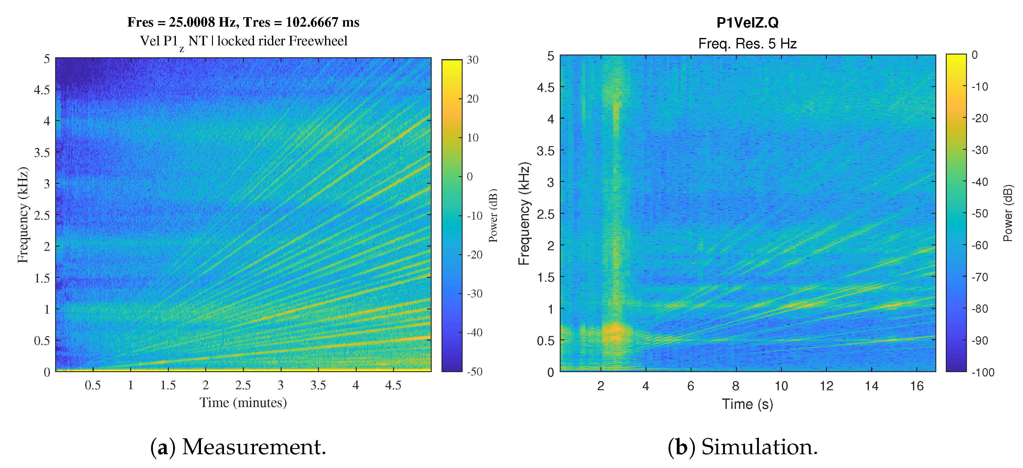
Figure 25.
Spectrogram of a ramp-up operation of the e-bike drive unit analysed at . An approximate correspondence can be assumed but is not significant.
Figure 25.
Spectrogram of a ramp-up operation of the e-bike drive unit analysed at . An approximate correspondence can be assumed but is not significant.
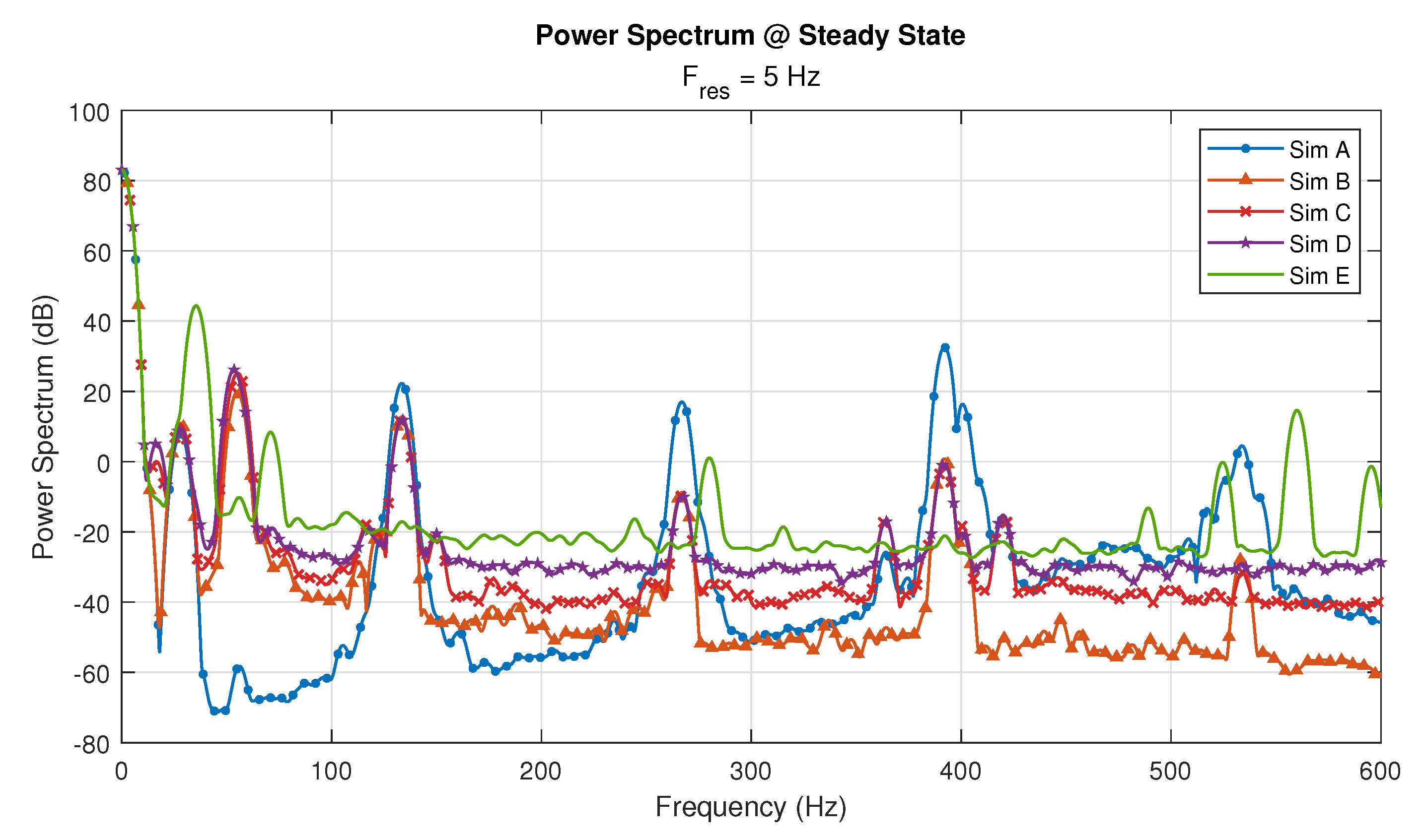
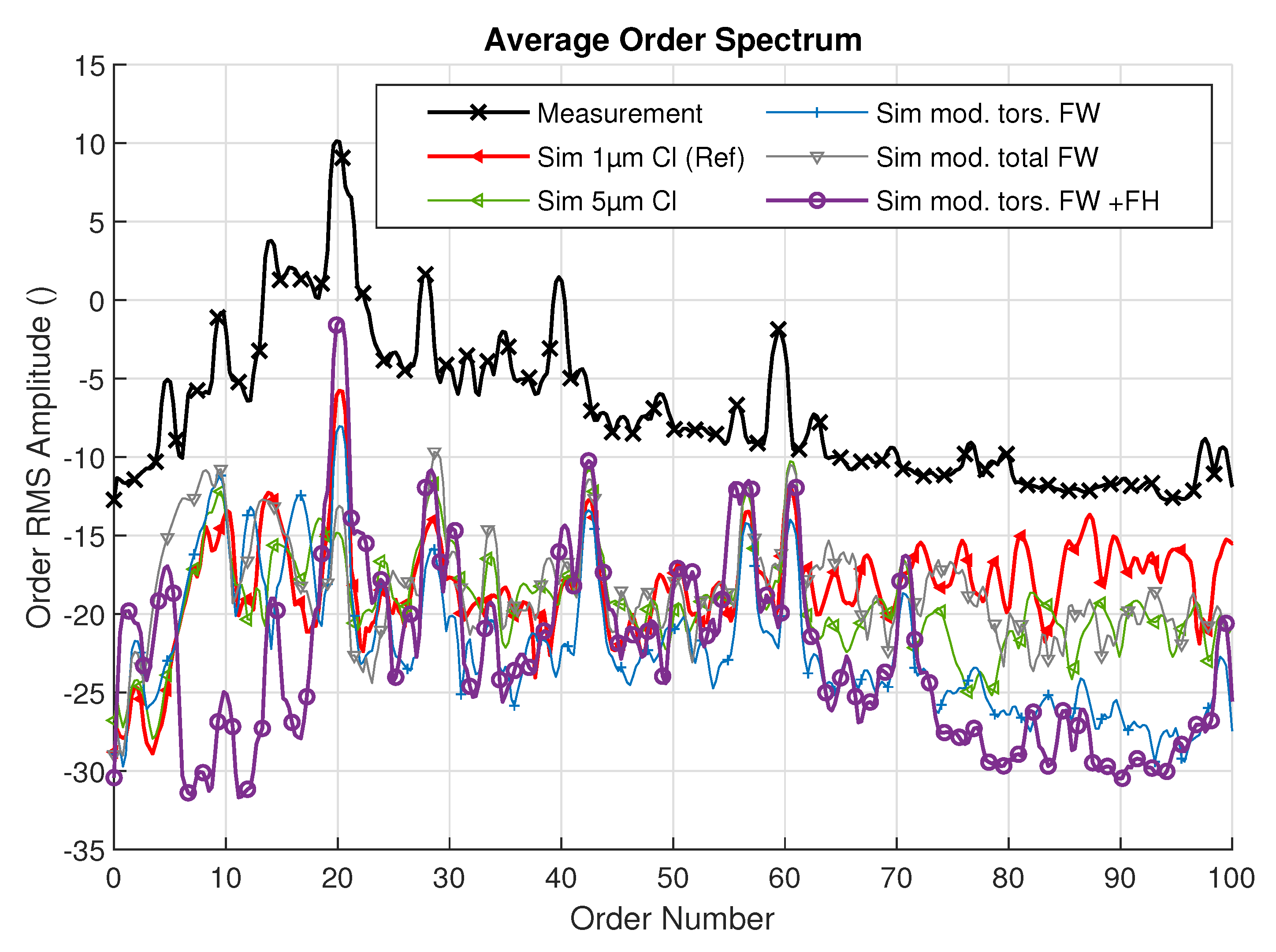
Figure 26.
Average order spectrum from different simulations and one measurement in comparison.
Figure 26.
Average order spectrum from different simulations and one measurement in comparison.
Table 1.
Description of the e-bike drive unit component’s function in the system and its NVH significance.
Table 1.
Description of the e-bike drive unit component’s function in the system and its NVH significance.
| Designation | Component Function and System Compliance | NVH Significance |
|---|
| Engine freewheel | Decouples the torque of the rotor uni-directional from the pedalling torque of the rider. The decoupling allows the resistance torque created by the gear transmission to avoid being dragged along when pedalling without engine support. | No noises are known due to the clamping mode of operation. |
| Rider freewheel | Decouples the rider’s pedalling torque uni-directional from the torque of the chain wheel, resulting from the bicycle chain force. It allows the chain to spin while the pedal remains in a fixed position. | There is a clicking sound when the freewheel opens due to the form-fitting mode of action. |
| Electrical motor (rotor and stator) | Generates a torque to support the rider’s pedalling torque. Requires special controlling of the system, as the timing when the rider is pedalling is indeterminate. | The motor vibrations lead to direct acoustic sound emissions, including the pulse width modulation, which controls the average power delivered by the electrical signal. |
| Gear stage (shafts, gears and bearings) and chain | Transfers and increases the rotor torque by the gear ratio. Decreases the revolution speed. | The tooth meshing of the gears induces rolling and sliding vibrations. Over-roll frequencies of the bearings are negligible to perceive. The chain braces the system and indicates vibration forces. |
| Housing | The housing absorbs the rotor dynamic forces transmitted by the bearings. It must resist the rider’s weight, the overall system torque and emerging dynamical forces. | The housing is mounted directly to the e-bike frame without the possibility of further acoustic sealing. Moreover, the stator is assembled directly inside the housing, whose vibrations during operation result in structure-borne acoustic emission. |
Table 2.
Mesh information and calculation time from linear perturbation step of processed FEM structures with tetrahedral elements of type C3D10.
Table 2.
Mesh information and calculation time from linear perturbation step of processed FEM structures with tetrahedral elements of type C3D10.
| Designation | Global Mesh Size | Number of Nodes | Number of Elements | Total CPU Time | Wallclock Time 1 |
|---|
| Rotor | ≤1.7 | 57,110 | 39,029 | 2.23 × 10 s | ≈1 min |
| Rotorshaft | ≤0.75 | 171,936 | 118,871 | 1.32 × 10 s | ≈6 min |
| Gearwheel | ≤1.5 | 54,842 | 35,724 | 8.30 × 10 s | ≈1 min |
| Driveshaft | ≤2.0 | 687,359 | 437,595 | 7.61 × 10 s | ≈28 min |
| Test rig | ≤4.0 | 420,354 | 285,390 | 1.82 × 10 s | ≈8 min |
| Housing | ≤3.9 | 426,763 | 249,725 | 2.29 × 10 s | ≈16 min |
Table 3.
Convergence studies by analysing the mesh size impact towards the solution accuracy and the computational time exemplarily on the rotorshaft. There are no more modes until 20 kHz.
Table 3.
Convergence studies by analysing the mesh size impact towards the solution accuracy and the computational time exemplarily on the rotorshaft. There are no more modes until 20 kHz.
| Run | Global Mesh Size | 1st Mode | Relative Deviation 1 | Total CPU Time | Wallclock Time |
|---|
| 1 | 1.5 s | 9539.6 Hz | 0.2% | 8.5 × 10 | ≈1 min |
| 2 | 0.75 s | 9520.5 Hz | 0.07% | 1.32 × 10 | ≈ 6 min |
| 3 | 0.375 | 9513.3 Hz | - | 6.50 × 10 | ≈167 min |
Table 4.
Used parameter values as reference for input within the eMBD simulation.
Table 4.
Used parameter values as reference for input within the eMBD simulation.
| Parameter Name | Parameter Value | Related Parts |
|---|
| Solver HHT 1 | error , max step , | Holistic model |
| Steps size output | | |
| Duration (1 s Ref) | Calculation time ≤ 2 h | |
| Structural damping 2 | 2% | Shafts, Gear bodies, Housing |
| Gear damping | variable (damping Ns/mm, ) | Gear contact |
| Gear stiffness | variable | Gear tooth |
| Bearing damping | variable (max. Ns/mm) | Bearing |
| Bearing stiffness | variable (max. N/mm) | Bearing |
| Freewheel damping | <1.0 Nmms/∘ | Engine freewheel |
| Freewheel stiffness | variable | Engine freewheel |
| Torque Rotor 3 | <5000 Nmm | Holistic model |
| Speed Rotor (RPM) 3 | <3000 1/min | Holistic model |
Table 5.
Metrics to align measurement and simulation results.
Table 5.
Metrics to align measurement and simulation results.
| Designation | Initial Conditions | Analysis Method |
|---|
| Steady state | Constant RPM, different load | Power Spectral Density (PSD) |
| Ramp up | Increasing RPM, different load | PSD Spectrogram |
| Order spectrum |
Table 6.
Simulations of different states used for verification of the model.
Table 6.
Simulations of different states used for verification of the model.
| Simulation, Variant | Gears | Shafts | Bearings | Freewheel | Torque |
|---|
| A | flex tooth | rigid | revolute joints | none | const. |
| B | flex tooth | rigid | revolute joints | rigidity 1 | const. |
| C | flex tooth | flex | joints 2 | rigidity | const. |
| D | flex tooth | flex | flex | rigidity | const. |
| E | flex tooth | flex | flex | rigidity | EMAG |
| (F) 3 | flex tooth | flex | flex | rigidity | EMAG |
| (G) 4 | flex tooth | flex | flex | rigidity | EMAG |
Table 7.
Comparison of the rotational oscillation from both the simulation and the measurement at similar speed.
Table 7.
Comparison of the rotational oscillation from both the simulation and the measurement at similar speed.
| Designation | Frequency, Measurement [Hz] | Frequency, Simulation [Hz] | Deviation [%] 4 |
|---|
| 1. RPM 1 | 27.7 | 28.4 | 2.53 |
| 2. RPM | 56.6 | 56.0 | −1.06 |
| 3. RPM | 84.1 | 84.1 | 0.00 |
| 4. 2 RPM | 112.2 | 113.8 | 1.43 |
| 5. RPM | 140.4 | 139.1 | −0.93 |
| 1. 1st gear stage (GS) | 133.4 | 134.1 | 0.53 |
| 6. RPM | 168.0 | 166.3 | −1.01 |
| 7. RPM | 195.4 | 196.5 | 0.56 |
| 8. RPM | 224.5 | 225.0 | 0.22 |
| 9. RPM | 252.3 | 251.6 | −0.27 |
| 10. RPM | 280.5 | 280.9 | 0.01 |
| SubH 3 1st GS (+20 Hz) | 153.0 | 155.8 | 1.83 |
| 2. 1st GS | 267.2 | 268.1 | 0.34 |
| 1. 2nd GS | 392.4 | 393.8 | 0.36 |
| 1. Electro-magnetic (EMAG) | 561.6 | 562.3 | 0.12 |
| SubH 2 EMAG | 533.4 | 536.2 | 0.52 |
| SubH 3 EMAG | 504.4 | 504.9 | 0.10 |
| SubH 4 EMAG | 477.1 | 479.5 | 0.50 |


