
A Two-Period Model of Coastal Urban Adaptation Supported by Climate Services


1
Climate Service Center Germany (GERICS), Helmholtz-Zentrum Hereon, Fischertwiete 1, 20095 Hamburg, Germany
2
Research Group Climate Change and Security (CLISEC), Institute of Geography, Center for Earth System Research and Sustainability (CEN), Universität Hamburg, Grindelberg 5/7, 20144 Hamburg, Germany
*
Author to whom correspondence should be addressed.
†
Current address: Institute of Coastal Systems—Analysis and Modeling, Helmholtz-Zentrum Hereon, Max-Planck-Straße 1, 21502 Geesthacht, Germany.
Urban Sci. 2022, 6(4), 65; https://doi.org/10.3390/urbansci6040065
Submission received: 15 June 2022
/
Revised: 13 August 2022
/
Accepted: 19 August 2022
/
Published: 23 September 2022
(This article belongs to the Special Issue Coastal Urban Dynamics under Climate Change)
Abstract
:Coastal zones are experiencing rapid urbanization at unprecedented rates. At the same time, coastal cities are the most prone to climate-related vulnerability, including impacts of sea-level rise and climate-related coastal hazards under the present and projected future climate. Decision making about coastal urban climate adaptation can be informed by coastal climate services based on modeling tools. We develop a two-period coastal urban adaptation model in which two periods—the present and the future—are distinguished. In the model, a city agent anticipates sea-level rise and related coastal flood hazards with adverse impacts in the future period that, through damages, will reduce the urban income. However, the magnitude of future sea-level rise and induced damages are characterized by uncertainty. The urban planning agent has to make an investment decision under uncertainty: whether to invest in climate adaptation (in the form of construction of coastal protection) or not, and if so, how much. The decision making of the urban agent is derived from intertemporal maximization of expected time-discounted consumption. An exact solution in the closed form is derived for an analytically tractable particular case, for which it is shown that investment decisions depend discontinuously on the value of a single non-dimensional model indicator. When this indicator exceeds a certain threshold value, the urban agent discontinuously switches from the ‘business-as-usual’ (BaU) strategy when no adaptation investment is taken to a proactive adaptation. The role of coastal climate services in informing the decision making on adaptation strategies is discussed.
1. Introduction
In a modern, rapidly urbanizing world, coastal zones are experiencing particularly high urbanization rates [1,2]. At the same time, these rapidly developing coastal urban areas are increasingly vulnerable to sea-level rise and climate-related coastal hazards [3,4,5,6,7,8,9]. This requires proactive climate adaptation of coastal cities [10], which can be supported by coastal climate services [11,12], a specific subdomain of climate services [13,14,15,16,17,18] that supports climate-informed decision making in coastal zones using climate knowledge.
To inform climate adaptation in coastal urban areas, it is necessary to understand both regional climate change and coastal urban systems. Urban modeling can substantially support the latter task. In view of the high complexity of urban systems, it is not surprising that many paradigms for urban modeling have evolved over time, with no single methodology capable of monopolizing or at least dominating the market. In fact, each of these complementary approaches successfully describes its own facets of complex urban dynamics. Socio-natural systems in general, and coastal urban systems in particular, can be modeled with optimization models [19,20,21]; system dynamics [22,23,24,25,26]; growth-diffusion models [27,28]; actor-based system dynamics modeling [29,30,31]; the VIABLE modeling framework [32,33,34]; agent-based modeling [35,36,37]; cellular automata [38,39,40,41,42]; social network analysis [43]; advanced methods of urban network analysis [44,45,46]; and many other modeling approaches. In the present paper, we adopt the first of the approaches listed above and develop a simple optimization model of a coastal city adapting to climate change under uncertainty. We have chosen the optimization modeling approach to explore under which conditions a fully rational actor described within a traditional economic modeling paradigm will choose a proactive coastal urban adaptation strategy.
Possible responses of coastal urban areas to climate adaptation challenge can include such versatile measures as traditional coastal defenses [47,48,49,50], nature-based solutions [51,52,53], and managed retreat and relocation of urban areas further inland [1]. The present paper is focused on traditional coastal defenses, including their strong points such as rich experience of construction projects at various scales, established engineering guidelines, and high effectiveness at preventing damage during extreme events [54]. It should be mentioned that similar models can be developed for other coastal adaptation options, as well.
In the present paper, we develop a simple discrete-time coastal urban adaptation model, where the urban agent has to make a decision on climate adaptation investment under uncertainty. The decision making of the urban agent is derived from intertemporal maximization of expected time-discounted urban consumption affected by climate damages in the future period. We also discuss, within the modeling framework developed, the role of coastal climate services in informing the decision making on possible urban adaptation strategies.
The model developed in the present paper has certain similarities to a one-step optimization global climate-economy model developed by Rovenskaya (2011) [55]. In particular, both models focus on two discrete-time moments: present and uncertain future, and are based on a one-sector growth model where annual GDP is split between consumption and investment. However, no explicit climate adaptation or mitigation options have been considered in the cited paper, while the focus of our research is on exploring the local coastal urban adaptation strategies and the role of coastal climate services in informing their development.
The rest of the paper is organized as follows. In Section 2, we provide a brief overview of the two-period coastal urban adaptation model and present the model equations. Section 3 is devoted to an in-depth analysis of an analytically tractable particular case of the model. Based on this analysis, in Section 4, we discuss the role of coastal climate services for decision making with regard to urban adaptation. Section 5 summarizes the main features of the reported coastal urban adaptation model, highlights the finding of a discontinuous change from a ‘business-as-usual’ (BaU) strategy to proactive adaptation measures conditional to a non-dimensional model indicator, and provides an outlook for possible further development of the model.
2. Methods
2.1. Overview of the Coastal Urban Adaptation Model
A coastal urban adaptation model to be developed might be considered as a ‘toy’ intertemporal optimization model. The model time is discrete, and only two periods are considered: the present () and the future ().
The coastal city is considered a closed economy affected by adverse climate change impacts in the future period. Within each period, the city generates income Y. The current version of the model does not describe the economic growth of the city, and in the absence of climate change impacts, the income in the future would be the same as it is at present:
Following this assumption, all income in the future period is consumed. In general, all present income can be also consumed. However, in the future period, the coastal city anticipates being affected by climate change, leading to sea-level rise (SLR) and climate-related coastal hazards. These will cause climate damage to the city, reducing the urban income at . Therefore, consumption in the future (equal, by assumption, to income in the future) will also be reduced, if the city does not take adaptation measures now.
Accordingly, the city may choose to take adaptation measures. This means that at , part of the urban income can be channeled in adaptation investment (in the form of coastal protection construction), at the expense of consumption. Coastal protection construction can reduce the future climate damage to the city, and therefore offset the reduction of future consumption caused by SLR. (Formally, within the simplistic modeling scheme proposed, the reduction of future consumption can be completely eliminated, provided that investment is sufficiently high. In a more realistic model setup, the uncertainty about the future SLR impacts will, of course, remain).
However, the current investment decision has to be taken under uncertainty. Among the multiple sources of uncertainty for long-term decision making of this kind, the following two factors can be highlighted:
- i.
- The quantitative projections of future SLR provided by climate science are uncertain;
- ii.
- Future climate damage is also assessed with substantial uncertainty.
Of particular importance for the project within which this modeling study has been conducted is the process of translation of climate science information into actionable knowledge. Accordingly, within the proposed probabilistic modeling scheme, we will primarily focus on the issue (i). However, we will also briefly tackle the issue (ii) in Section 4.
The decision making on coastal urban adaptation strategies can be efficiently supported by coastal climate services. In the present paper, we address the following dimension of climate services: how can the climate information—in this case on projected SLR and climate-related coastal hazards, including the uncertainty analysis of future climate projections—inform the decision making of urban agent(s) regarding possible adaptation responses?
2.2. Model Equations
Based on climate projections, the coastal city expects that in the period , it will suffer from climate damages caused by SLR. However, the magnitude of future SLR, and the future damages at , are still uncertain at , when the city has to make an investment decision regarding the coastal protection construction.
The city can invest part of its income at , equal to I, when building the coastal protection. The remaining is consumed at . Therefore, the budget constraint at is
At , the city does not make any investment and consumes everything it can. The consumption at is therefore equal to
where is the damage function from SLR and climate-related coastal hazards the city experiences at . Dependent on climate change and the urban adaptation policy, both affecting the argument of the climate damage function at , it can be either (no damage at all at ) or (damage does occur).
The investment I leads to the construction of coastal protection at with the ‘efficient height’ equal to
where is the inverse cost of construction of one unit of height of coastal protection.
The damage function in Equation (3) depends on the difference between the (exogenous) SLR and the efficient height of coastal protection (all variables at ). In Section 3.1 below, we will explicitly define the damage function for an analytically tractable particular case.
The SLR in the future, relative to its present value, is uncertain at present. We assume that climate projections deliver its probability density function (PDF) .
The city maximizes the expected discounted consumption. In a continuous-time intertemporal optimization problem, the discounted consumption would take the form
where r is the discount rate. In our simple two-period discrete model, an analogue of Equation (5) would be
where is the discount factor.
As depends on , C in Equation (6) also depends on : .
In summary, the city faces the following maximization problem: to choose the investment I in such a way that the expected discounted consumption
is maximized.
Explicitly, it can be easily shown that, under assumptions made,
and the latter expression should be maximized as a function of the investment I.
While the model equations presented in this Section combine many ideas from traditional economic modeling, notably from economic growth theory, the authors see their main contribution in the detailed tractable analysis of a particular case of the climate damage function reported in Section 3 below, and also in exploring the role of uncertainty of climate science information in the process of development of coastal climate services (Section 4 below).
3. Results
3.1. An Analytically Tractable Particular Case: Simplifying Assumptions
We will now consider in detail an analytically tractable particular case of the coastal urban adaptation model presented in the previous section. In order to demonstrate the main findings from the model in as technically simple a way as possible, we make the following simplifying assumptions:
Assumption 1.
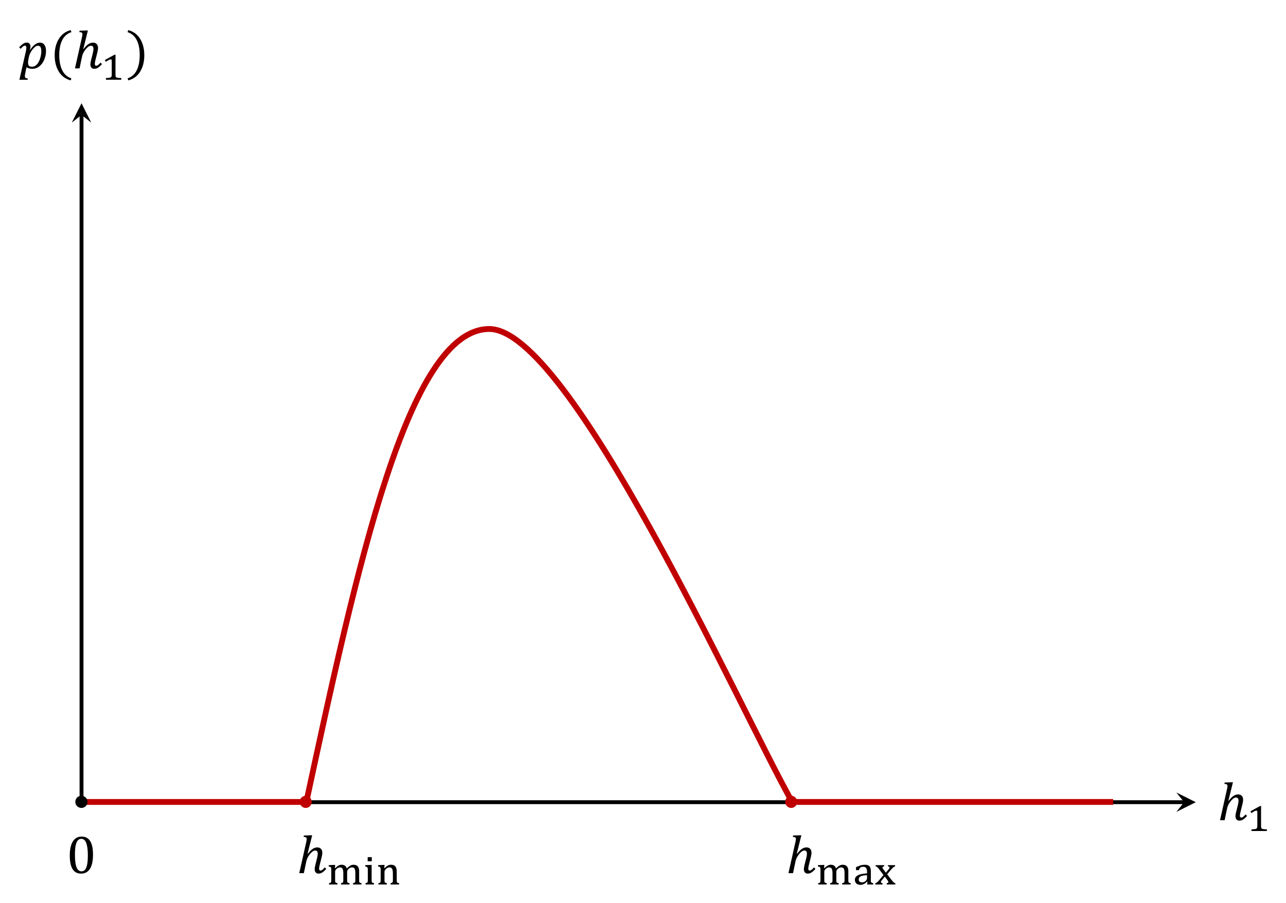
A finite PDF is chosen for .
That means that there is a constant lower bound and upper bound for SLR (where , such that
Assumption 2.
The magnitude of future SLR is uncertain; however, it is certain that some SLR will occur.
Combined with Assumption 1, this means that
A sketch of a PDF for SLR satisfying the Assumptions 1 and 2 is provided in Figure 1.
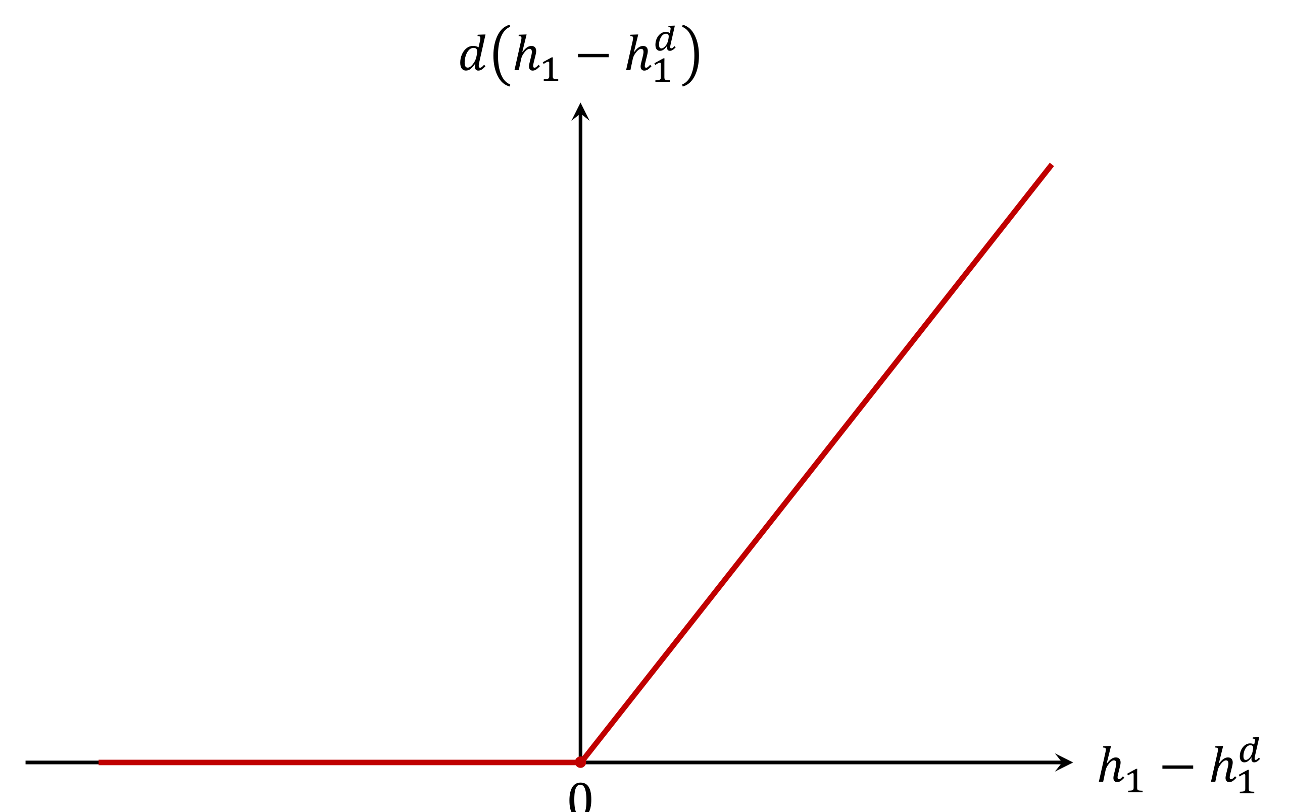
Assumption 3.
The damage function is piecewise linear and takes the explicit form
where the (positive) slope γ defines how rapidly the damage increases with growing SLR (Figure 2).
3.2. Solution in a Particular Case
We now maximize provided by Equation (8) under simplifying assumptions made in Section 3.1.
After some calculations (see the detailed derivations in the Section 3.3 below), we arrive at the following main result.
Based on the following analysis, we introduce a new non-dimensional indicator which contains key parameters of the model:
and the cumulative distribution function (CDF) corresponding to PDF ,
With the newly introduced indicator B and the CDF, the conditions for optimal investment can be determined as:
where is a solution of the (algebraic) equation
In other words, the case corresponds to the ‘business-as-usual’ (BaU) strategy with no adaptation investment at all, while the opposite case corresponds to proactive adaptation in the form of coastal protection construction.
The following conditions are favorable to the BaU case : the discount factor is low (the future is not so important for the urban decision maker); the urban income is not so large; the construction of coastal protection implies high costs; the growth of damages with SLR is slow. Opposite conditions are favorable to choosing the proactive adaptation strategy.
3.3. Derivation of Model Solution in a Particular Case
In the present Section, we provide the derivation of the main result stated in Section 3.2.
In Equation (8), in view of Assumption 1 (finiteness of the PDF),
By performing in Equation (16) integration by parts, we get:
To find the maximum of , we will differentiate Equation (8) over I. To do this, we differentiate Equation (19) over I and notice that
This yields
Consider the specific form of the damage function given by Equation (11) (Assumption 3). Given that the damage function is assumed to be piecewise linear, for its first and second derivative, we get
where, in Equation (22), is the Heaviside step function,
and in Equation (23), is the Dirac delta function,
By substituting Equations (22)–(23) into Equation (21), we get
where a product of two Heaviside step functions in the first term in the r.h.s of Equation (26) has been introduced to account for finite limits of integration in Equation (21).
Equation (26) can be simplified to the form
With the help of Equation (27), we easily find from Equation (8) that
where the indicator B has been defined in Equation (12).
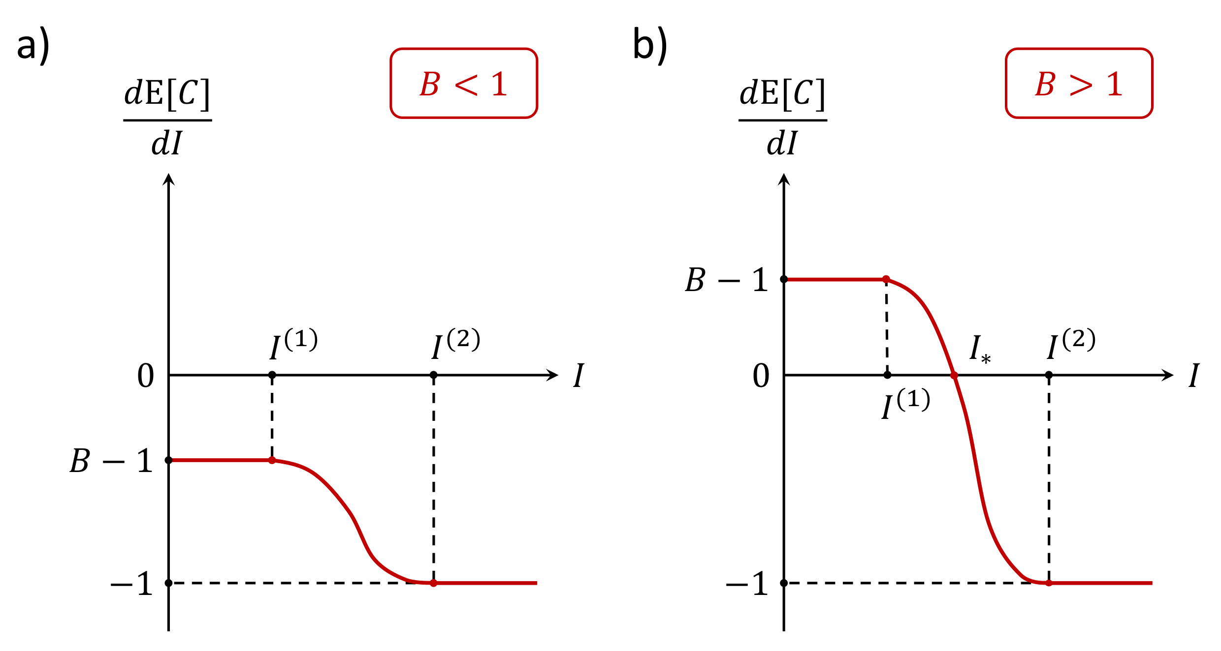
We now define two threshold investment levels
Explicitly, with new notations introduced, Equation (28) takes the form
As any CDF is a non-decreasing function of its argument, it can be easily seen that the derivative is a continuous non-increasing function. If , it is equal to a constant value , that, dependent on the value of the indicator B, can be negative, zero, or positive. If , it is equal to and is definitely negative. In between, if , the derivative is continuously changing within these limits.
Therefore, two cases are possible (Figure 3).
If (Figure 3a), the derivative is always negative. This means that is a decreasing function of I, and, therefore, to maximize , (no investment at all) should be chosen. This is the BaU strategy with no adaptation.
If (Figure 3b), the derivative is initially positive, then it starts decreasing and eventually becomes negative. This means that initially increases with I, but then starts decreasing. The point where the derivative is equal to zero corresponds to a maximum of . This point corresponds to the solution of Equation (15). However, we should also take into account the budget constraint (Equation (2)). So, we should choose either or, in case does not satisfy the budget constraint, the maximum possible investment compatible with the budget constraint, . Overall, this yields Equation (14).
In accordance with Equations (29) and (31), and also with Figure 3b, if the value of the indicator B only slightly exceeds its ‘threshold’ value , then the chosen investment only slightly exceeds and, therefore, the efficient height of coastal protection only slightly exceeds , guaranteeing zero damage under the most optimistic SLR scenario only (at minimum possible SLR). A hypothetical case would similarly correspond to the opposite limit , guaranteeing zero damage at maximum possible SLR (and, therefore, at any SLR). Since the infinite value of B is not possible, this implies that maximum protection would not be taken.
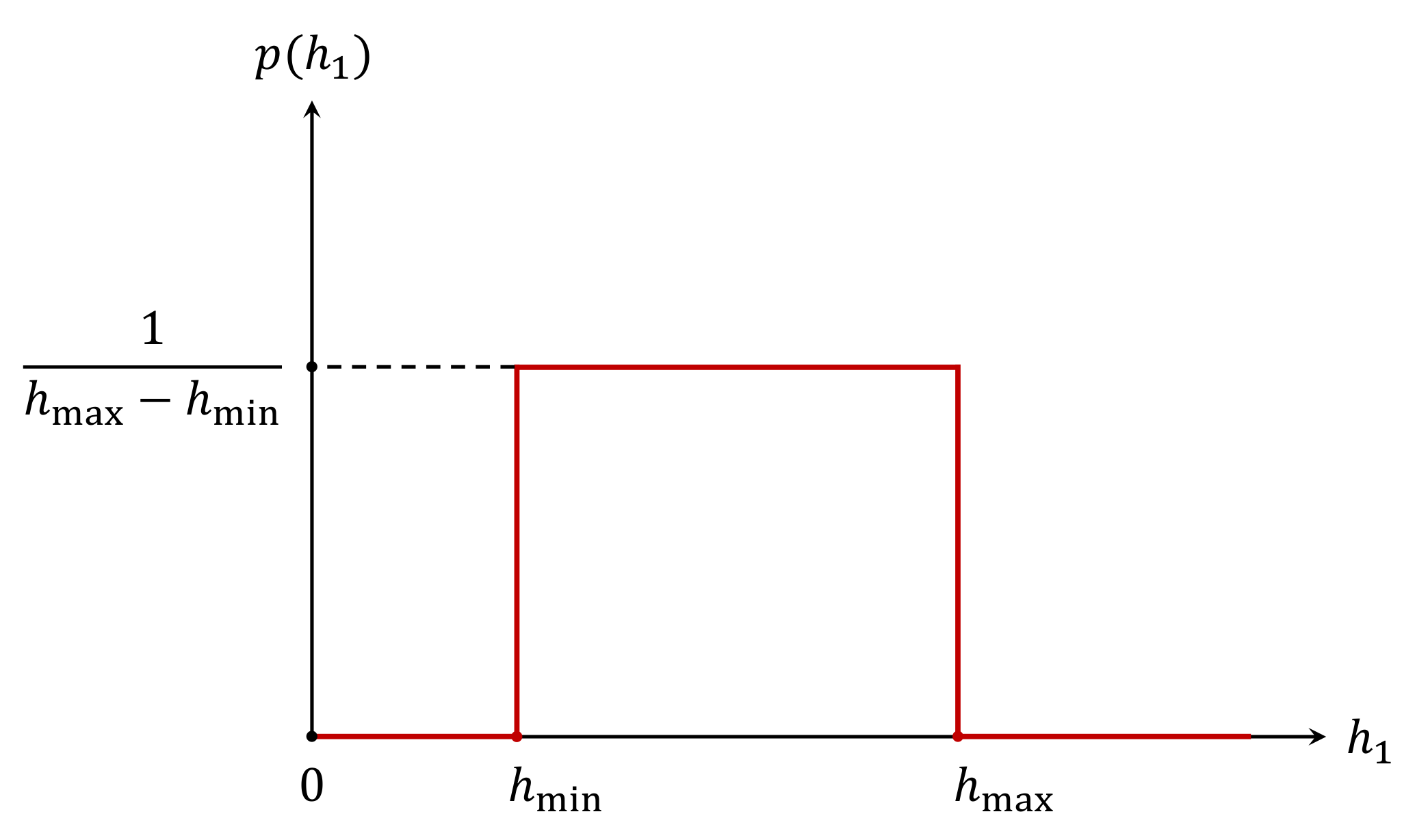
3.4. An Exemplary Uniform PDF for SLR
Consider now, for simplicity, a case in which a uniform PDF (Figure 4) is chosen for :
It should be noticed here that real PDFs for SLR provided by climate projections of course take a more complex form [3,4,5], and so an example (32) should be considered as illustrative to show the benefit of an explicit solution.
Then Equation (15) to find can be easily solved explicitly, and the solution takes the form
We will discuss Equation (33) in the next Section.
4. Discussion: The Role of Coastal Climate Services
Within the simple modeling scheme developed in the present paper, coastal climate services can provide valuable information for the urban decision maker regarding:
- i.
- The form and parameters of the probability distribution function (PDF) for SLR;
- ii.
- The form and parameters of the climate damage function.
As mentioned above, this information is inevitably uncertain. In view of this, we now briefly discuss the sensitivity of solutions derived in Section 3 for the particular case of the presented model to the values of parameters potentially delivered by coastal climate services.
Firstly, we note that an expression (12) for the non-dimensional model indicator B does not include any information on a particular PDF for SLR chosen. No matter what particular form of the PDF we choose, and what values we assign to parameters specifying this probability distribution, the indicator B will be the same (as soon as the chosen PDF satisfies the Assumptions 1 and 2 made in Section 3.1, while the damage function satisfies Assumption 3). At the same time, the slope of the damage function does affect the value of indicator B. As the threshold value for B separating the investment and the no-investment case is simply a non-dimensional constant (equal to one), this means that in the proposed simplistic modeling scheme, the ‘economic’ information embedded in the damage function affects the point where the BaU strategy is abandoned and the adaptation investment is triggered, while the ‘physical’ information embedded in the PDF for SLR does not. However, if a decision on adaptation investment is taken, the value of optimal investment is of course affected by both the ‘economic’ (damage function) and the ‘physical’ (PDF for SLR) parameters.
If the modeled coastal urban system is within the domain of the parameter space where , the decision making is robust with respect to PDF for SLR (as there is zero investment anyway under BaU, it is not important to know the exact parameters of PDF for SLR).
However, the situation changes if . Then, if the decision maker does not know the exact parameter values of the PDF, the chosen investment can maximize the expected consumption only by coincidence.
Consider again an example with a uniform PDF (Equation (32)) and the resultant optimal investment (Equation (33)). Let . If , then (Equation (29)), and, therefore, is sensitive to and insensitive to . In the opposite case of , we have ; is insensitive to and sensitive to . This means that, dependent on the ‘economic’ parameters of the urban system, there might be more demand for the ‘physical’ information either on the ‘best-case’ (low-end) or the ‘worst-case’ (high-end) SLR projections.
For the uniform PDF (Equation (32)), the case leads to the coastal protection height being exactly the average of minimum and maximum possible SLR levels, as follows from Equation (33).
More realistic models would undoubtedly bring more details (and, probably, certain revisions) in a brief sketch of the role of coastal climate services outlined in the present section.
5. Conclusions and Outlook
In the present paper, we developed a simple two-period coastal adaptation model and explored analytically tractable particular conditions in detail. Despite the simplicity of the proposed modeling scheme, the decision making of the urban agent demonstrates a non-trivial discontinuous dependence on model parameters. When a non-dimensional model indicator defined by Equation (12) exceeds its threshold value, the ‘business-as-usual’ (BaU) strategy with zero investment in climate adaptation discontinuously changes to a proactive adaptation strategy with an investment exceeding a certain positive lower bound. The proposed model is substantially probabilistic, and we discussed the role of coastal climate services in providing the information relevant for decision making on coastal urban adaptation under inevitable multi-level uncertainty.
The simple model developed in the present paper can be further extended in a number of directions. One methodological development would be to consider a similar intertemporal optimization problem in continuous time, and in a more general setting maximizing the discounted utility of consumption, and not merely the discounted consumption itself. At the same time, as discussed in the Introduction section, the optimization framework is not at all the only possible formalism of describing the decision making of model agent(s). To achieve a broader perspective on describing the adaptive agent decision making, we are planning to explore a modified coastal urban adaptation model within the VIABLE modeling framework [34], involving multiple agents who can interact in conflict or cooperate in taking joint action. More added value can be provided by considering realistic PDFs for SLR provided by climate projections within the proposed modeling scheme or non-linear damage functions. Including the description of economic growth in the model is also important. Last but not least, as also discussed in the Introduction section, building coastal protection is not the only possible adaptation option for a city facing sea-level rise. Cities might be urged to implement other measures, including managed retreat and population relocation [1]. Based on our previous experience exploring a portfolio of coastal urban adaptation options within the VIABLE modeling framework [56,57] we are planning to extend the presented modeling scheme to include a choice between alternative adaptation options, or a combination of them. This approach may be also applicable to other cases of adaptation to environmental challenges, including promising innovative coastal urban adaptation measures other than traditional construction of hard defences. All these developments towards more detailed and realistic modeling are planned for future work.
Author Contributions
Conceptualization, D.V.K. and J.S.; methodology, D.V.K. and J.S.; formal analysis, D.V.K.; investigation, D.V.K.; writing—original draft preparation, D.V.K. and J.S.; writing—review and editing, D.V.K. and J.S.; project administration, D.V.K. and J.S.; funding acquisition, D.V.K. and J.S. All authors have read and agreed to the published version of the manuscript.
Funding
This work was conducted and financed within the framework of the Helmholtz Institute for Climate Service Science (HICSS), a cooperation between Climate Service Center Germany (GERICS) and Universität Hamburg, Germany [Project ‘Modeling Urban dynamics affected by Climate Change for Coastal Spatial planning and management’ (MUCCCS)].
Institutional Review Board Statement
Not applicable.
Informed Consent Statement
Not applicable.
Data Availability Statement
Data is contained within the article.
Acknowledgments
The authors are grateful to Laurens Bouwer, Shubhankar Sengupta and the three anonymous reviewers of the manuscript for their helpful comments. The authors would also like to thank the participants of the NDC 2020 Conference (23–25 November 2020), EGU General Assembly 2021 (19–30 April 2021) and ECSA 58-EMECS 13 Conference (6–9 September 2021) where this research has been presented [58], and of GERICS Team Meetings (GERICS, Helmholtz-Zentrum Hereon, Hamburg, Germany), for the stimulating feedback received.
Conflicts of Interest
The authors declare no conflict of interest.
Abbreviations
The following abbreviations are used in this manuscript:
| BaU | ‘business-as-usual’. |
| CDF | Cumulative distribution function. |
| Probability density function. | |
| SLR | Sea-level rise. |
| VIABLE | Values and Investments from Agent-Based interaction and Learning in |
| Environmental systems. |
References
- Rosenzweig, C.; Solecki, W.D.; Romero-Lankao, P.; Mehrotra, S.; Dhakal, S.; Ibrahim, S.A. Climate Change and Cities: Second Assessment Report of the Urban Climate Change Research Network; Cambridge University Press: Cambridge, UK, 2018. [Google Scholar]
- Yang, L.E.; Chan, F.K.S.; Scheffran, J. Climate change, water management and stakeholder analysis in the Dongjiang River basin in South China. Int. J. Water Resour. Dev. 2018, 34, 166–191. [Google Scholar] [CrossRef]
- IPCC. Climate Change 2021: The Physical Science Basis. Contribution of Working Group I to the Sixth Assessment Report of the Intergovernmental Panel on Climate Change; Cambridge University Press: Cambridge, UK; New York, NY, USA, 2021. [Google Scholar] [CrossRef]
- IPCC. Sea level rise and implications for low-lying islands, coasts and communities. In The Ocean and Cryosphere in a Changing Climate: Special Report of the Intergovernmental Panel on Climate Change; Cambridge University Press: Cambridge, UK, 2022; pp. 321–446. [Google Scholar] [CrossRef]
- Pugh, D.; Woodworth, P. Sea-Level Science: Understanding Tides, Surges, Tsunamis and Mean Sea-Level Changes; Cambridge University Press: Cambridge, UK, 2014. [Google Scholar] [CrossRef]
- Hoegh-Guldberg, O.; Jacob, D.; Taylor, M.; Bolaños, T.G.; Bindi, M.; Brown, S.; Camilloni, I.A.; Diedhiou, A.; Djalante, R.; Ebi, K.; et al. The human imperative of stabilizing global climate change at 1.5 °C. Science 2019, 365, eaaw6974. [Google Scholar] [CrossRef]
- Von Szombathely, M.; Albrecht, M.; Antanaskovic, D.; Augustin, J.; Augustin, M.; Bechtel, B.; Bürk, T.; Fischereit, J.; Grawe, D.; Hoffmann, P.; et al. A conceptual modeling approach to health-related urban well-being. Urban Sci. 2017, 1, 17. [Google Scholar] [CrossRef]
- Yang, L.E.; Scheffran, J.; Süsser, D.; Dawson, R.; Chen, Y.D. Assessment of flood losses with household responses: Agent-based simulation in an urban catchment area. Environ. Model. Assess. 2018, 23, 369–388. [Google Scholar] [CrossRef]
- Smirnov, V.; Ma, Z.; Volchenkov, D. Invited article by M. Gidea Extreme events and emergency scales. Commun. Nonlinear Sci. Numer. Simul. 2020, 90, 105350. [Google Scholar] [CrossRef] [PubMed]
- IPCC. Climate Change 2022: Impacts, Adaptation, and Vulnerability. Contribution of Working Group II to the Sixth Assessment Report of the Intergovernmental Panel on Climate Change; Cambridge University Press: Cambridge, UK; New York, NY, USA, 2022; in press. [Google Scholar]
- Cortekar, J.; Bender, S.; Brune, M.; Groth, M. Why climate change adaptation in cities needs customised and flexible climate services. Clim. Serv. 2016, 4, 42–51. [Google Scholar] [CrossRef]
- Rölfer, L.; Winter, G.; Máñez Costa, M.; Celliers, L. Earth observation and coastal climate services for small islands. Clim. Serv. 2020, 18, 100168. [Google Scholar] [CrossRef]
- Jacob, D.; Kotova, L.; Teichmann, C.; Sobolowski, S.P.; Vautard, R.; Donnelly, C.; Koutroulis, A.G.; Grillakis, M.G.; Tsanis, I.K.; Damm, A.; et al. Climate impacts in Europe under +1.5 °C global warming. Earth’s Future 2018, 6, 264–285. [Google Scholar] [CrossRef]
- Teichmann, C.; Bülow, K.; Otto, J.; Pfeifer, S.; Rechid, D.; Sieck, K.; Jacob, D. Avoiding extremes: Benefits of staying below +1.5 °C compared to +2.0 °C and +3.0 °C global warming. Atmosphere 2018, 9, 115. [Google Scholar] [CrossRef]
- Koldunov, N.V.; Kumar, P.; Rasmussen, R.; Ramanathan, A.; Nesje, A.; Engelhardt, M.; Tewari, M.; Haensler, A.; Jacob, D. Identifying climate change information needs for the Himalayan Region: Results from the GLACINDIA Stakeholder Workshop and Training Program. Bull. Am. Meteorol. Soc. 2016, 97, ES37–ES40. [Google Scholar] [CrossRef]
- Preuschmann, S.; Hänsler, A.; Kotova, L.; Dürk, N.; Eibner, W.; Waidhofer, C.; Haselberger, C.; Jacob, D. The IMPACT2C web-atlas—Conception, organization and aim of a web-based climate service product. Clim. Serv. 2017, 7, 115–125. [Google Scholar] [CrossRef]
- Akhtar, N.; Geyer, B.; Rockel, B.; Sommer, P.S.; Schrum, C. Accelerating deployment of offshore wind energy alter wind climate and reduce future power generation potentials. Sci. Rep. 2021, 11, 11826. [Google Scholar] [CrossRef]
- Weisse, R.; Bisling, P.; Gaslikova, L.; Geyer, B.; Groll, N.; Hortamani, M.; Matthias, V.; Maneke, M.; Meinke, I.; Meyer, E.; et al. Climate services for marine applications in Europe. Earth Perspect. 2015, 2, 3. [Google Scholar] [CrossRef]
- Nordhaus, W. A Question of Balance: Weighing the Options on Global Warming Policies; Yale University Press: New Haven, CT, USA, 2014. [Google Scholar]
- Landry, C.E. Coastal erosion as a natural resource management problem: An economic perspective. Coast. Manag. 2011, 39, 259–281. [Google Scholar] [CrossRef]
- Gopalakrishnan, S.; Landry, C.E.; Smith, M.D.; Whitehead, J.C. Economics of coastal erosion and adaptation to sea level rise. Annu. Rev. Resour. Econ. 2016, 8, 119–139. [Google Scholar] [CrossRef]
- Forrester, J.W. Urban Dynamics; MIT Press: Cambridge, MA, USA, 1969. [Google Scholar]
- Meadows, D.; Randers, J.; Meadows, D. Limits to Growth: The 30-Year Update; Chelsea Green Publishing Co.: Vermont, VT, USA, 2004. [Google Scholar]
- Fiddaman, T. Dynamics of climate policy. Syst. Dyn. Rev. 2007, 23, 21–34. [Google Scholar] [CrossRef]
- Hallegatte, S.; Ghil, M. Natural disasters impacting a macroeconomic model with endogenous dynamics. Ecol. Econ. 2008, 68, 582–592. [Google Scholar] [CrossRef] [Green Version]
- Kellie-Smith, O.; Cox, P.M. Emergent dynamics of the climate—Economy system in the Anthropocene. Philos. Trans. R. Soc. Math. Phys. Eng. Sci. 2011, 369, 868–886. [Google Scholar] [CrossRef]
- O’Neill, W.D. Estimation of a logistic growth and diffusion model describing neighborhood change. Geogr. Anal. 1981, 13, 391–397. [Google Scholar] [CrossRef]
- Kovalevsky, D.V.; Volchenkov, D.; Scheffran, J. Cities on the coast and patterns of movement between population growth and diffusion. Entropy 2021, 23, 1041. [Google Scholar] [CrossRef] [PubMed]
- Hasselmann, K. Detecting and responding to climate change. Tellus Chem. Phys. Meteorol. 2013, 65, 20088. [Google Scholar] [CrossRef]
- Hasselmann, K.; Kovalevsky, D.V. Simulating animal spirits in actor-based environmental models. Environ. Model. Softw. 2013, 44, 10–24. [Google Scholar] [CrossRef]
- Hasselmann, K.; Cremades, R.; Filatova, T.; Hewitt, R.; Jaeger, C.; Kovalevsky, D.; Voinov, A.; Winder, N. Free-riders to forerunners. Nat. Geosci. 2015, 8, 895–898. [Google Scholar] [CrossRef]
- Scheffran, J. Conflict and cooperation in energy and climate change: The framework of a dynamic game of power-value interaction. In Jahrbuch für Neue Politische Ökonomie, Band 20: Power and Fairness; Holler, M., Kliemt, H., Schmidtchen, D., Streit, M., Eds.; Mohr Siebeck: Tübingen, Germany, 2002. [Google Scholar]
- Scheffran, J. Adaptive management of energy transitions in long-term climate change. Comput. Manag. Sci. 2008, 5, 259–286. [Google Scholar] [CrossRef]
- BenDor, T.K.; Scheffran, J. Agent-Based Modeling of Environmental Conflict and Cooperation; CRC Press: Boca Raton, FL, USA, 2018. [Google Scholar]
- Benenson, I.; Torrens, P. Geosimulation: Automata-Based Modeling of Urban Phenomena; John Wiley & Sons: New York, NY, USA, 2004. [Google Scholar]
- Filatova, T.; Verburg, P.H.; Parker, D.C.; Stannard, C.A. Spatial agent-based models for socio-ecological systems: Challenges and prospects. Environ. Model. Softw. 2013, 45, 1–7. [Google Scholar] [CrossRef]
- Aerts, J.C.; Botzen, W.J.; Clarke, K.C.; Cutter, S.L.; Hall, J.W.; Merz, B.; Michel-Kerjan, E.; Mysiak, J.; Surminski, S.; Kunreuther, H. Integrating human behaviour dynamics into flood disaster risk assessment. Nat. Clim. Change 2018, 8, 193–199. [Google Scholar] [CrossRef]
- Tobler, W.R. Cellular geography. In Philosophy in Geography; Springer: New York, NY, USA, 1979; pp. 379–386. [Google Scholar]
- White, R.; Engelen, G. Cellular automata and fractal urban form: A cellular modelling approach to the evolution of urban land-use patterns. Environ. Plan. Econ. Space 1993, 25, 1175–1199. [Google Scholar] [CrossRef] [Green Version]
- Hewitt, R.; van Delden, H.; Escobar, F. Participatory land use modelling, pathways to an integrated approach. Environ. Model. Softw. 2014, 52, 149–165. [Google Scholar] [CrossRef]
- Sekovski, I.; Armaroli, C.; Calabrese, L.; Mancini, F.; Stecchi, F.; Perini, L. Coupling scenarios of urban growth and flood hazards along the Emilia-Romagna coast (Italy). Nat. Hazards Earth Syst. Sci. 2015, 15, 2331–2346. [Google Scholar] [CrossRef]
- Song, J.; Fu, X.; Gu, Y.; Deng, Y.; Peng, Z.R. An examination of land use impacts of flooding induced by sea level rise. Nat. Hazards Earth Syst. Sci. 2017, 17, 315–334. [Google Scholar] [CrossRef]
- Rodriguez-Lopez, J.M.; Schickhoff, M.; Sengupta, S.; Scheffran, J. Technological and social networks of a pastoralist artificial society: Agent-based modeling of mobility patterns. J. Comput. Soc. Sci. 2021, 4, 681–707. [Google Scholar] [CrossRef]
- Volchenkov, D.; Blanchard, P. Markov chain methods for analyzing urban networks. J. Stat. Phys. 2008, 132, 1051–1069. [Google Scholar] [CrossRef]
- Blanchard, P.; Volchenkov, D. Mathematical Analysis of Urban Spatial Networks; Springer Science & Business Media: New York, NY, USA, 2008. [Google Scholar]
- Volchenkov, D.; Smirnov, V. The City of Lubbock is running away. Integration and isolation patterns in the wandering city. J. Vib. Test. Syst. Dyn. 2019, 3, 121–132. [Google Scholar] [CrossRef]
- Vrijling, J.; van Hengel, W.; Houben, R. Acceptable risk as a basis for design. Reliab. Eng. Syst. Saf. 1998, 59, 141–150, Risk Perception Versus Risk Analysis. [Google Scholar] [CrossRef]
- Dean, R.G.; Dalrymple, R.A. Coastal Processes with Engineering Applications; Cambridge University Press: Cambridge, UK, 2004. [Google Scholar]
- Sorensen, R.M. Basic Coastal Engineering; Springer: New York, NY, USA, 2006. [Google Scholar]
- Kind, J. Economically efficient flood protection standards for the Netherlands. J. Flood Risk Manag. 2014, 7, 103–117. [Google Scholar] [CrossRef]
- World Bank Group. Managing Coasts with Natural Solutions: Guidelines for Measuring and Valuing the Coastal Protection Services of Mangroves and Coral Reefs; Technical Report; The World Bank: Washington, DC, USA, 2016. [Google Scholar]
- Schueler, K. Nature-Based Solutions to Enhance Coastal Resilience; Technical Report; Inter-American Development Bank: Washington, DC, USA, 2017. [Google Scholar]
- Costanza, R.; Anderson, S.J.; Sutton, P.; Mulder, K.; Mulder, O.; Kubiszewski, I.; Wang, X.; Liu, X.; Pérez-Maqueo, O.; Luisa Martinez, M.; et al. The global value of coastal wetlands for storm protection. Glob. Environ. Change 2021, 70, 102328. [Google Scholar] [CrossRef]
- OECD. Responding to Rising Seas; Technical Report; OECD: Paris, France, 2019. [Google Scholar] [CrossRef]
- Rovenskaya, E. One-step optimization model of warming-driven damage of economic growth. In Proceedings of the DEGIT Conference Papers c016_062, DEGIT, Dynamics, Economic Growth, and International Trade, St. Petersburg, Russia, 8–9 September 2011; Available online: https://econpapers.repec.org/paper/degconpap/c016_5f062.htm (accessed on 18 August 2022).
- Sengupta, S.; Scheffran, J.; Kovalevsky, D. Agent adaptation in an urban coastal scenario: Applying the VIABLE Framework. In Proceedings of the DKT-12-22, 12. Deutsche Klimatagung, Online, 15–18 March 2021. [Google Scholar] [CrossRef]
- Sengupta, S.; Scheffran, J.; Kovalevsky, D. A Single-Agent Urban Coastal Adaptation Model: Adaptive decision-making within the VIABLE modeling framework. In Proceedings of the EGU21-12752, EGU General Assembly 2021, Online, 19–30 April 2021. [Google Scholar] [CrossRef]
- Kovalevsky, D.; Scheffran, J. A coastal urban adaptation model with time-discounting, optimizing and satisficing decision making. In Proceedings of the EGU21-12228, EGU General Assembly 2021, Online, 19–30 April 2021. [Google Scholar] [CrossRef]
Figure 1.
A sketch of a finite probability density function for sea-level rise satisfying the assumptions from Section 3.1.
Figure 1.
A sketch of a finite probability density function for sea-level rise satisfying the assumptions from Section 3.1.

Figure 2.
A piecewise linear climate damage function dependent on the difference between sea-level rise and the ‘efficient height’ of coastal protection (Equation (11)).
Figure 2.
A piecewise linear climate damage function dependent on the difference between sea-level rise and the ‘efficient height’ of coastal protection (Equation (11)).

Figure 3.
A derivative of expected discounted consumption over adaptation investment as a function of I. (a) A non-dimensional model indicator B given by Equation (12) obeys an inequality . (b) Same as (a), but for the opposite case .
Figure 3.
A derivative of expected discounted consumption over adaptation investment as a function of I. (a) A non-dimensional model indicator B given by Equation (12) obeys an inequality . (b) Same as (a), but for the opposite case .

Figure 4.
An exemplary uniform probability density function for sea-level rise.

Publisher’s Note: MDPI stays neutral with regard to jurisdictional claims in published maps and institutional affiliations. |
© 2022 by the authors. Licensee MDPI, Basel, Switzerland. This article is an open access article distributed under the terms and conditions of the Creative Commons Attribution (CC BY) license (https://creativecommons.org/licenses/by/4.0/).
Share and Cite
MDPI and ACS Style
Kovalevsky, D.V.; Scheffran, J. A Two-Period Model of Coastal Urban Adaptation Supported by Climate Services. Urban Sci. 2022, 6, 65. https://doi.org/10.3390/urbansci6040065
AMA Style
Kovalevsky DV, Scheffran J. A Two-Period Model of Coastal Urban Adaptation Supported by Climate Services. Urban Science. 2022; 6(4):65. https://doi.org/10.3390/urbansci6040065
Chicago/Turabian StyleKovalevsky, Dmitry V., and Jürgen Scheffran. 2022. "A Two-Period Model of Coastal Urban Adaptation Supported by Climate Services" Urban Science 6, no. 4: 65. https://doi.org/10.3390/urbansci6040065