Article

Automatic Identification of Auroral Substorms Based on Ultraviolet Spectrographic Imager Aboard Defense Meteorological Satellite Program (DMSP) Satellite

1
MNR Key Laboratory for Polar Science, Polar Research Institute of China, Shanghai 200136, China
2
Ocean College, Zhejiang University, Zhoushan 316021, China
3
School of Electronic Engineering, Xidian University, Xi’an 710071, China
4
Beijing Institute of Applied Meteorology, Beijing 100029, China
*
Author to whom correspondence should be addressed.
Universe 2023, 9(9), 412; https://doi.org/10.3390/universe9090412
Submission received: 30 March 2023 / Revised: 27 August 2023 / Accepted: 31 August 2023 / Published: 8 September 2023
(This article belongs to the Section Space Science)

Abstract

:
An auroral substorm is an important physical process of energy accumulation and explosive release in the Earth’s magnetosphere, and is an important research object of space environment monitoring and space weather warnings. A westward traveling surge (WTS) is a typical auroral physical process of an auroral substorm. Its static characteristic is auroral folding at the polar boundary of an auroral oval and its dynamic characteristic is the westward motion of auroral folding. According to the static characteristic of a WTS, we defined a set of feature parameters based on the morphology and designed a set of automatic detection and discrimination methods; that is, the WTS was identified by using the extracted features and pattern recognition approaches. This approach was tested by using the aurora data of the ultraviolet auroral spectral imager of the Defense Meteorological Satellite Program (DMSP) satellite. The results showed that the accuracy rate of automatic recognition was 61.39%~63.61% and the precision rate was 55.52%~57.92%. The experimental results showed that the approach was effective at detecting the typical characteristics of an auroral substorm (WTS).

1. Introduction

In the solar wind–magnetosphere–ionosphere coupling system, auroral substorms are an important manifestation of magnetosphere energy accumulation and explosive release, which can be used to study the interaction between solar wind and the magnetosphere as interplanetary magnetic field (IMF) ionospheric disturbance [1]. When a substorm occurs, it can have effects on communication in high-latitude regions and the operation of geosynchronous satellites [2]. Therefore, auroral substorms have been the subject of extensive interest and research in space physics.
Existing research on auroral substorms has mainly focused on the occurrence mechanism of substorms through case studies, simulating their physical processes. Pattern recognition is an artificial intelligence technique designed to automatically recognize and classify patterns or regularities in data, usually by extracting features from input data and then using machine learning algorithms to train models that can classify or predict new data. There are two types of identification approaches for substorm events in case studies. One is to use manual processing or pattern recognition to identify substorm events based on some space physical parameters related to substorms such as the interplanetary magnetic field (IMF), solar wind, and geomagnetic field parameters. Another is to use pattern recognition approaches to extract high-level semantic features of auroral images for the identification of substorm events; e.g., ultraviolet imager (UVI) data based on the polar satellites and all-sky imager (ASI) data based on an ASI [3].
At present, there are many works on substorm event identification approaches based on spatial physical parameters. The following works may be mentioned. Wang et al. [4] analyzed the variation pattern of the auroral electrojet (AE) index during substorms. Sutcliffe et al. [5] used a neural network and Pi2 pulsation index to detect and identify the onset of substorms. Murphy et al. [6] used wavelet changes and Pi1 and Pi2 pulsation indices to determine a substorm onset. Tokunaga et al. [7] detected a substorm onset by using the singular value change of ground magnetometer data. Kataoka et al. [8] used the Hilbert–Huang variation of geomagnetic pulsation data to analyze a substorm onset. Meng et al. [9] pointed out that measured spatial physical parameters and substorms do not correspond in time because the parameters are measured at the top of the magnetosphere and it takes some propagation time for them to affect the auroral parameters in the ionosphere, so it is difficult to identify substorms based on spatial physical parameters.
For the second type of substorm event identification, the optical observation of auroras [10,11,12] is an approach to observe the dynamics of auroral substorms. The following works on substorm identification from auroral images may be mentioned. Akasofu [13] defined phases of substorm development based on ground-based all-sky camera observations. Liou et al. [14] studied the growth phase of substorms using a satellite-borne ultraviolet imager. In order to more accurately discriminate substorm events, some scholars have used aurora images to detect substorms based on their features by using manual discrimination or pattern recognition approaches. Previous works that manually identified substorm events include: 1) Frey et al. [15] identified 4193 substorm events from ultraviolet auroral data from the IMAGE satellite. The criteria were, firstly, that significant localized auroral brightening must be observed in the auroral oval; secondly, that the localized brightening must extend to the polar boundary of the auroral oval and have a duration of at least 20 min in the direction of magnetic local time (MLT); and thirdly, that the interval between two separate substorms must be more than 30 min. 2) Liou [16] identified 2003 and 536 substorm events, respectively, from UVI data from the Polar satellite during its operation in the northern hemisphere (1996–2000) and in the southern hemisphere (from 2007 onwards). The criteria used were some improvements on Frey’s by firstly imposing a 10 min time interval for auroral spotting and secondly, not requiring the expansion area to reach the poleward boundary of the auroral oval but requiring it to be in the expansion range of the bright spot in the poleward direction for 1–2 magnetic latitude (MLAT) points. However, manual calibration is time-consuming and subject to subjective factors.
Based on the substorm development characteristic, Yang et al. [17] proposed an automatic detection approach for the substorm expansion phase onset. However, this approach is only suitable for continuous sequences of auroral image data such as the UVI of the Polar satellite with a sampling interval of more than ten seconds to several minutes; it is not suitable for the commonly used ultraviolet aurora data (the time interval between two adjacent frames is about 100 min and the dynamic process of the substorm cannot be observed) acquired by the ultraviolet spectral imagers of DMSP and Thermosphere Ionosphere Mesosphere Energetics and Dynamics (TIMED) satellites. However, the spatial resolution of auroral images obtained by low-orbit satellites such as DMSP and TIMED is much higher than that of the Polar satellite. The Polar satellite is a scientific experiment launched by NASA in February 1996 to study the magnetosphere and aurora in the polar region. The satellite has an elliptical orbit with an apogee of about 9 Earth radii, a perigee of about 1.8 Earth radii, and an orbital period of about 18 h. The Polar satellite has a spatial resolution of 24 km × 26 km~36 km × 40 km at altitudes greater than 6 Earth radii, while the DMSP satellites have a spatial resolution of 10 km × 10 km, much higher than the Polar satellite. Therefore, this paper proposes a new substorm detection approach for auroral image data with high spatial resolution but low temporal resolution. In an ultraviolet auroral image with low temporal resolution and high spatial resolution, the time interval between two adjacent frames is about one hour, so dynamic information such as the brightening of the auroral oval and polar expansion in the auroral image sequence cannot be extracted. However, due to their high spatial resolution, fine structures in auroral images can be obtained such as the WTS, which is a typical structure during the occurrence of substorms [18]. Therefore, it is possible to identify whether the current moment is in the substorm occurrence phase by detecting whether the image contains a WTS structure to achieve the purpose of automatic detection of substorms.
With the development of information science and artificial intelligence, pattern recognition approaches have achieved good results in the field of object detection. But the aurora image does not have a lot of identified data for deep learning models to train from. Studies have shown that [18] during an auroral substorm, an expanding motion of an auroral system located around the midnight sector generates rapid wavy motions of auroral arcs or bands that lie in the evening sector. This particular type of motion is called the WTS. However, the pattern recognition approach cannot directly detect a WTS structure according to this definition. The aim of this study was to identify substorm events from ultraviolet auroral images by extracting WTS features from these images.

2. Data and Approaches

2.1. Brief Description of a Substorm

In 1964, Akasofu [13] defined a substorm for the first time using data from several all-sky imagers, dividing it into two phases: the expansive and the recovery phases. At the onset of the expansive phase, energy stored in the magnetotail is released and the ionospheric auroras appear as an equatorward shift of the parallel auroral arcs in the pre-midnight sector, with a sudden increase in brightness in the auroral arc closest to the equator. Subsequently, the auroral bright spot increases in brightness and appears to expand in the polar and azimuthal directions until it expands to the polar boundary of the auroral oval or decreases in brightness and area. In the recovery phase, the bright spot of the aurora decreases in brightness and area to pre-substorm levels [19].
In 1970, Mcpherron [20] used ground-based magnetometer data to verify that a growth phase preceded the substorm expansive phase. Thus, the evolution of substorms can be divided into three phases: the growth phase, the expansive phase, and the recovery phase [21]. The growth phase is a phase of energy accumulation during which the nocturnal auroral arc moves towards the equator, but these motions are not evident in the global auroral oval image. The expansive phase initially manifests as a sudden brightening of the equatorward discrete auroral arc at midnight or a sudden appearance of an auroral arc. Generally, there is then a polar expansion of the aurora region and large-scale aurora folding occurs in the dusk sector. New aurora folding appears to the west of the old aurora folding, accompanied by the disappearance of the old aurora folding. This westward expansion of aurora folding is known as the WTS. The phase after the polar expansion of the auroral region reaches the highest latitude and begins to contract is called the recovery phase of the auroral substorm. During the substorm recovery phase, the WTS continues to expand westward and eventually degenerates into irregular-banded auroras [22].
A WTS is a typical structure of an auroral substorm. We can achieve the goal of substorm identification by detecting the WTS. The WTS has obvious dynamic and static characteristics and, as low temporal resolution images do not capture the dynamics of auroras, the characteristic presented by observing the substorm in such images is called the static characteristic. The static characteristic includes the boundary characteristic and brightness characteristic. The boundary characteristic refers to the steep and folding polar boundary of the auroral oval. The brightness characteristic refers to the poleward boundary intensification (PBI) near the steep western boundary, which is generally believed to be related to enhanced local magnetic reconnection [23,24,25,26].

2.2. Datasets

In 1973, the U.S. Department of Defense launched the DMSP program to monitor space weather and research the solar–Earth space environment. For this purpose, a series of polar orbiting satellites operating in sun-synchronous orbits were launched, with an orbital height of 840 km, an orbital inclination of 98.9 degrees, and an orbital period of 101 min [27]. The DMSP satellites carry a variety of observation instruments to monitor the plasma environment in near-Earth space. Among them, the F17, F18, and F19 satellites currently in orbit (launched in October 2003, November 2006, and October 2009, respectively) carry a Special Sensor Ultraviolet Spectral Imager (SSUSI), which can realize the simultaneous observation of the ionosphere/thermosphere/mesosphere (ITM) and auroras [28].
SSUSI is a far-ultraviolet scanning imaging spectrometer, which can detect 5 spectral bands of ultraviolet auroras (HI-Lyman α 121.6 nm, OI 130.4 nm, OI 135.6 nm, N2-Lyman Birge Hopfield short (LBHS) 140–160 nm, and N2-Lyman Birge Hopfield long (LBHL) 160–180 nm) for synchronous scanning imaging observations. Its mirror rotates perpendicular to the satellite orbit, and each scan produces an image of 16 × 156 pixels. Due to the DMSP satellites requiring 20–30 min to fly over the polar regions, SSUSI can obtain an image covering 1/3 to 1/2 of the auroral oval with a spatial resolution of about 10 × 10 km for each polar flight [29]. The left of Figure 1 shows the intensity distribution image of the ultraviolet aurora in the LBHL band obtained by the DMSP F16 satellite flying over the Arctic at 04:45:22–05:07:51 Universal Time (UT) on 29 March 2004. This image covers the aurora oval in the 07–21 MLT sectors where there is a bright aurora region within the 19–20 MLT sectors and the 60–80° MLAT region. The polar boundary of the aurora in this region has a static characteristic. The aurora structure is a WTS.
The orbit of the DMSP F16 satellite is along the 21–09 MLT direction; its auroral images can cover more 18–24 MLT sectors than other DMSP satellites, which is the dominantly occurrent region of a WTS. Therefore, the auroral image data obtained by DMSP F16 are used in this article. Moreover, in order to avoid the impact of sunlight, this article uses the January, February, October, November, and December LBHL band auroral data of the DMSP F16 satellite from 2004 to 2007. In this period of data, 366 auroral images including a WTS and 533 auroral images without a WTS were obtained through manual interpretation for the study of substorm automatic recognition. The definition of the WTS described in this paper can be applied to any data, but the method proposed in this paper is aimed at the characteristics of a WTS from SSUSI data. All the data used in this paper have been uploaded to https://zenodo.org/record/8082849 (26 June 2023) [30].

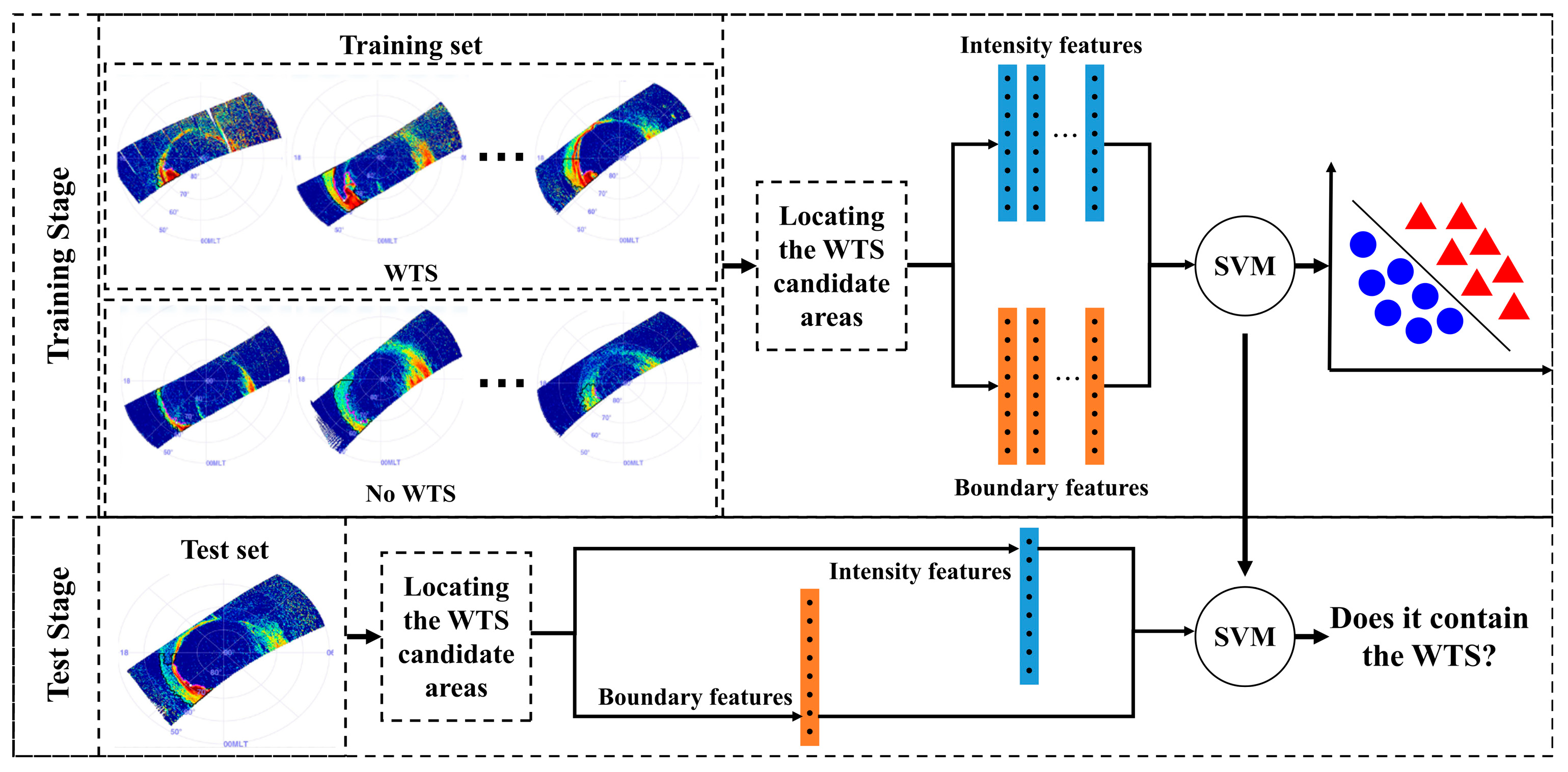
2.3. Automatic Identification of an Auroral Substorm

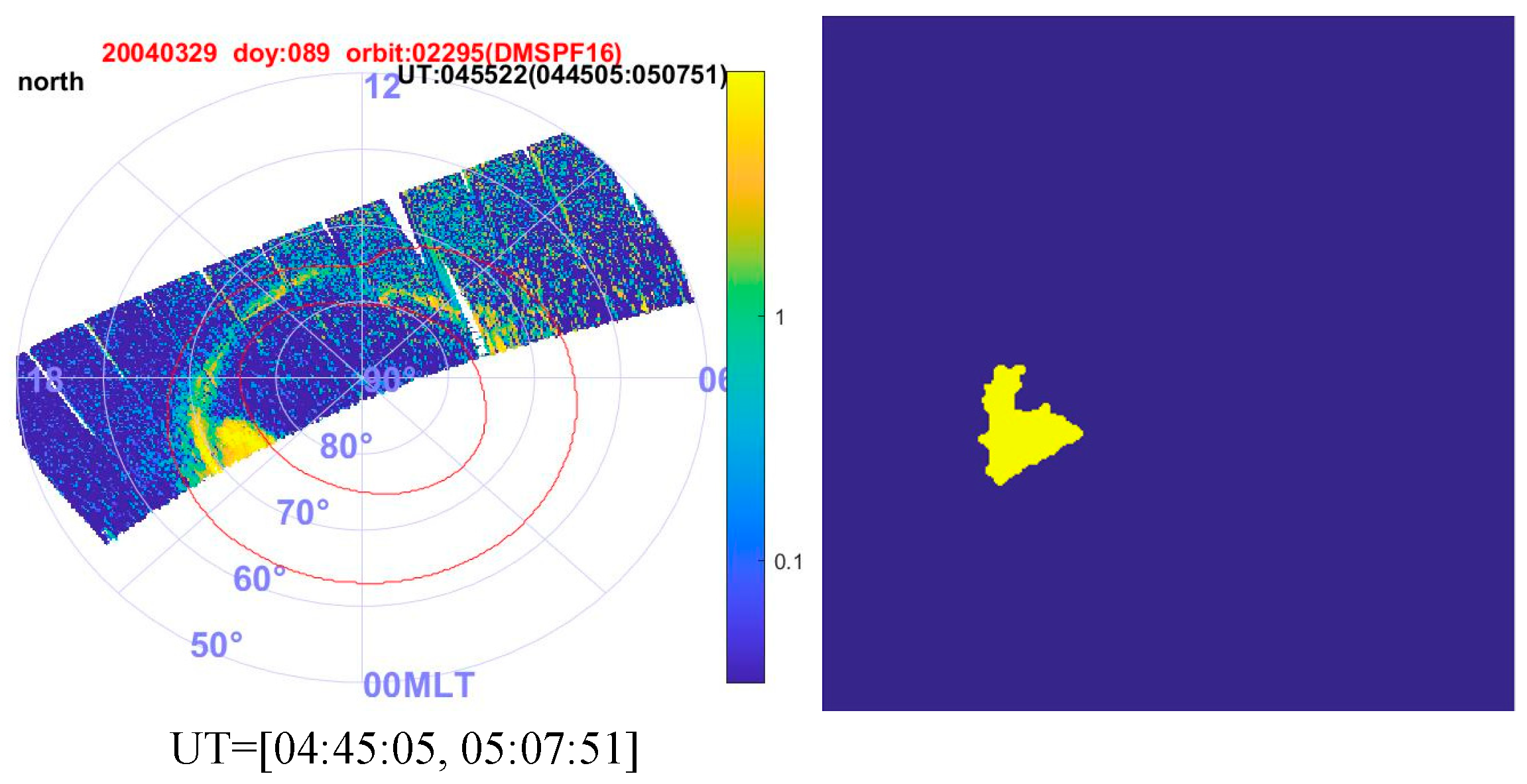
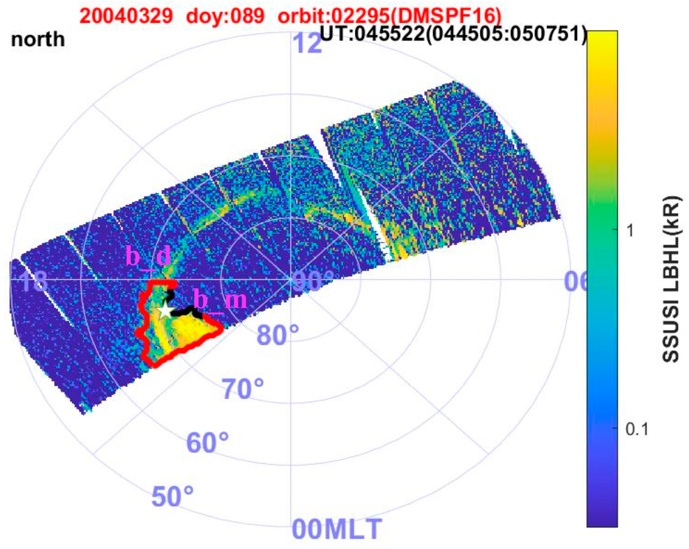
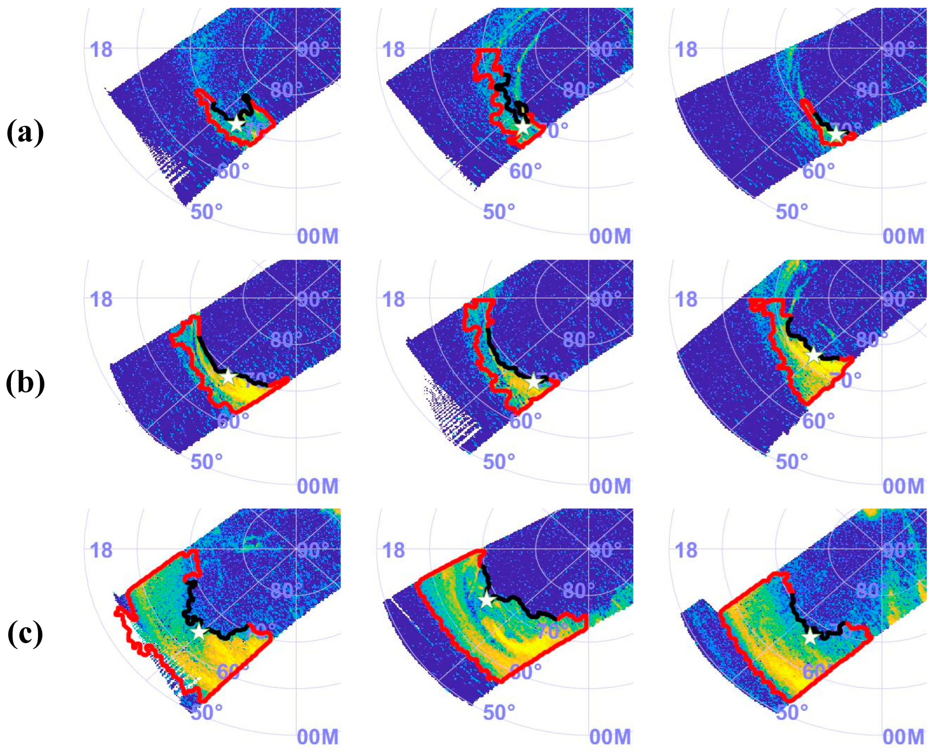
2.3.1. Locating the Candidate Region of a WTS

The WTS generally occurs in the duskside to midnight auroral oval (18–24 MLT sectors), so it is only necessary to process the images between 18 MLT and 24 MLT to obtain the possible occurrence area of a WTS. First, using our previously developed UV aurora oval boundary segmentation approach [12,31,32,33,34], we obtained the auroral oval region within the 18–24 MLT sectors. The yellow area to the right of Figure 1 is the auroral oval region within the 18–24 MLT sectors after the segmentation of the boundaries of the auroral oval in the left image of Figure 1.
The fold of a WTS is the static characteristic of the WTS. It has been found that the fold of a WTS is located on the polar boundary of the auroral oval where the value difference between MLT and MLAT is the largest. Therefore, the steps to determine the candidate region of a WTS are as follows:
(1)
Determine the polar boundary (PB) of the auroral oval fragment (yellow area to the right of Figure 1);
(2)
Locate the position of the PB with the largest value difference between MLT and MLAT, which is named as the extreme value point in this paper. Its vicinity is the candidate region for the WTS. The location of the extreme value point is shown in Equation (1).
P * = argmax P N ( MLT P MLAT P )
where N denotes the set of coordinate positions of the auroral region’s poleward boundary and P* denotes the extreme points in the set of poleward boundary positions. The position of P* is shown by the white asterisk in Figure 2. MLTP represents the MLT of the polar boundary points and MLATP represents the MLAT of the polar boundary points.
As the structure and size of a WTS varies depending on the phase it is in, two-thirds of the polar boundary on the duskside and midnight side of the extreme value point are, respectively, taken as the polar boundary of the WTS candidate region and the corresponding sector as a WTS candidate region. The part of the WTS boundary on the duskside of the extreme value point is called the duskside boundary (b_d) and the part on the midnight side is called the midnight boundary (b_m), as shown by the black curves on each side of the white asterisks in Figure 2, respectively.

2.3.2. Extracting the Features of a WTS

According to the definition of a WTS, there is a steep boundary to the east of its extremum point and there is a poleward boundary enhancement in its structure. Based on this, this section presents a set of empirical algorithms to extract the boundary features and intensity features of WTS candidate regions.
First, the boundary features of the WTS candidate region are extracted. The items of the boundary features are as follows:
(1)
The MLT mean difference (diff_MLT_md) and MLAT mean difference (diff_MLAT_md) between the midnight side and the duskside boundaries are calculated.
diff _ MLT _ md = E P b _ m ( MLT P ) E P b _ d ( MLT P )
diff _ MLAT _ md = E P b _ m ( MLAT P ) E P b _ d ( MLAT P )
where E (⋅) denotes the finding of the mean value.
(2)
The first derivative mean of MLAT to MLT at the midnight side boundary (mean_d1_d), the first derivative mean of MLAT to MLT at the duskside boundary (mean_d1_m), and the difference between them (diff_d1_md) are calculated.
mean _ d 1 _ d = E P b _ d ( 𝜕 MLAT P 𝜕 MLT P )
mean _ d 1 _ m = E P b _ m ( 𝜕 MLAT P 𝜕 MLT P )
diff _ d 1 _ md = mean _ d 1 _ m mean _ d 1 _ d
(3)
The mean of the absolute value of the first derivative of MLAT to MLT for the midnight boundary (mean_absd1_d), the mean of the absolute value of the first derivative of MLAT to MLT for the duskside boundary (mean_absd1_m), and the difference between them (diff_absd1_md) are calculated.
mean _ absd 1 _ d = E P b _ d ( | 𝜕 MLAT P 𝜕 MLT P | )
mean _ absd 1 _ m = E P b _ m ( | 𝜕 MLAT P 𝜕 MLT P | )
diff _ absd 1 _ md = mean _ absd 1 _ m mean _ absd 1 _ d
(4)
The second derivative mean of MLAT to MLT for the midnight boundary (mean_d2_d), the second derivative mean of MLAT to MLT for the duskside boundary (mean_d2_m), and the difference between them (diff_d2_md) are calculated.
mean _ d 2 _ d = E P b _ d ( 𝜕 2 MLAT P 𝜕 MLT P 2 )
mean _ d 2 _ m = E P b _ m ( 𝜕 2 MLAT P 𝜕 MLT P 2 )
diff _ d 2 _ md = mean _ d 2 _ m mean _ d 2 _ d
(5)
The mean of the absolute value of the second derivative of MLAT to MLT for the midnight boundary (mean_absd2_d), the mean of the absolute value of the second derivative of MLAT to MLT for the duskside boundary (mean_absd2_m), and the difference between them (diff_absd2_md) are calculated.
m e a n _ a b s d 2 _ d = E P b _ d ( | 𝜕 2 M L A T P 𝜕 M L T P 2 | )
m e a n _ a b s d 2 _ m = E P b _ m ( | 𝜕 2 M L A T P 𝜕 M L T P 2 | )
d i f f _ a b s d 2 _ m d = m e a n _ a b s d 1 _ m m e a n _ a b s d 1 _ d
(6)
The histogram distributions of the duskside boundary with ten equal parts are calculated, along with the MLT distribution features (counts_MLT_d), the MLAT distribution features (counts_MLAT_d), the MLAT to MLT first derivative distribution features (counts_d1_d), and the MLAT to MLT second derivative distribution features (counts_d2_d).
(7)
The histogram distributions of midnight side boundary with ten equal parts are calculated, along with the MLT distribution features (counts_MLT_m), the MLAT distribution features (counts_MLAT_m), the MLAT to MLT first derivative distribution features (counts_d1_m), and the MLAT to MLT second derivative distribution features (counts_d2_m).
Second, the intensity features of the WTS candidate region are extracted. The WTS candidate region is evenly divided into 12 sectors according to the MLT and each sector is evenly divided into 6 small sectors according to the range of the MLAT. The mean intensity (m_i) of each small sector and the intensity growth ratio (i_r) in the poleward direction are calculated as follows:
m _ i n , l = E ( I n , l ) ,   n = 1 , 2 , , 12 ; l = 1 , 2 , , 6
i _ r n , l = m _ i n , l + 1 m _ i n , l m _ i n , l ,   n = 1 , 2 , , 12 ; l = 1 , 2 , , 5
where In,l is the auroral intensity in the lth small sector of the nth sector.
Finally, the features of the WTS candidate region are composed of boundary features and intensity features as follows:
F = [ diff _ MLT _ md ,   diff _ MLAT _ md , mean _ d 1 _ d , mean _ d 1 _ m , diff _ d 1 _ md , mean _ absd 1 _ d , mean _ absd 1 _ m , diff _ absd 1 _ md , mean _ d 2 _ d , mean _ d 2 _ m , diff _ d 2 _ md , mean _ absd 2 _ d , mean _ absd 2 _ m , diff _ absd 2 _ md , count _ MLT _ d , count _ MLAT _ d , count _ d 1 _ d , count _ d 2 _ d , count _ MLT _ m , count _ MLT _ m , count _ d 1 _ m , count _ d 2 _ m , i _ r ]

2.3.3. Determining the Structures of a WTS

First, aurora images containing a WTS and aurora images without a WTS were manually selected and the corresponding features were extracted, respectively. The extracted features and corresponding labels were inputted into a support vector machine (SVM) [35] classifier for training to obtain the trained classifier. The features corresponding with the test data were extracted and fed into the trained classifier to obtain the category corresponding with the test data. The entire process flow is given in Figure 3.

3. Experimental Results and Analysis

3.1. Objective Evaluation

A total of 366 auroral images including a WTS and 533 auroral images without a WTS were selected for the experiment. Therefore, the number of features extracted for both cases with and without a WTS were 366 and 533, respectively.
The extracted feature samples with a WTS and without a WTS were randomly divided into a training dataset and test dataset according to a different ratio. We used the training dataset to train the SVM classifier and used the trained SVM classifier to classify the test set to test the effectiveness of the SVM classifier. During the classification test, the SVM classifier automatically identified the aurora images as two types of auroral image with and without a WTS, respectively, according to the features of the samples. However, compared with the actual manual recognition results, there were four situations in the recognition results of the SVM classifier; namely:
a.
The actual positive samples were predicted to be positive samples by the classifier; i.e., the aurora image actually contained a WTS and the SVM classifier recognized it as containing a WTS.
b.
The actual positive samples were predicted to be negative samples by the classifier; i.e., the aurora image actually contained a WTS and the SVM classifier recognized that it did not contain a WTS.
c.
The actual negative samples were predicted to be positive samples by the classifier; i.e., the aurora image did not contain a WTS and the SVM classifier recognized it as containing a WTS.
d.
The actual negative samples were predicted to be negative samples by the classifier; i.e., the aurora image did not contain a WTS and the SVM classifier recognized that it did not contain a WTS.
According to these four situations, we calculated the accuracy rate (Raccuracy) (the ability of the classifier to identify the correctness of the overall sample), recall rate (Rrecall) (the ability of the classifier to correctly predict the full degree of positive samples), miss rate (Rmiss) (the ability of the classifier to correctly predict the purity of negative samples), false-alarm rate (Rfalse-alarm) (the ability of the classifier to correctly predict the purity of positive samples), and precision rate (Rprecision) (the ability of the classifier to correctly predict the accuracy of positive samples) of the classification results. These five evaluation indicators identified the effectiveness of the SVM classifier accordingly. Accuracy is a measure of the overall performance of a classifier, while precision is a measure of the accuracy of a classifier when predicting a positive class. For the purpose of this paper, the precision represents the accuracy of detecting images containing a WTS. The formulas for calculating these five indicators were as follows:
R accuracy = a + d a + b + c + d
R recall = a a + b
R miss = b a + b
R false alerm = c a + c
R precision = a a + c
Fox example, when the ratio of a training set to a test was 1:9, a confusion matrix including the four situations was obtained, as shown in Table 1. The values of the five indicators were an accuracy rate of 63.00%, a recall rate of 49.66%, a misdetection rate of 50.34%, a false-alarm rate of 44.48%, and a precision rate of 55.52%.
We tested the performance of the SVM classifier under different train–test data ratios (from 1:9 to 5:5). In order to avoid the unrepresentative results of a single test, 10 tests were repeated under the same train/test data ratio and the average values of the five indicators were used as the representative indexes of the train/test data ratio (see Table 2). The experimental results showed that the accuracy rate and precision rate of our SVM classifier were relatively stable, no matter how much the train–test ratio changed; their values were mainly 61.39%~63.61% and 55.52%~57.92%, respectively. However, the value of the miss rate (recall rate) greatly fluctuated, ranging from 50.34% to 76.05% (from 23.95% to 49.66%). Compared with the previous approaches [17] used to detect substorm events from UVI images, the precision of the proposed approach increased by about 7%.

3.2. Analysis of Results

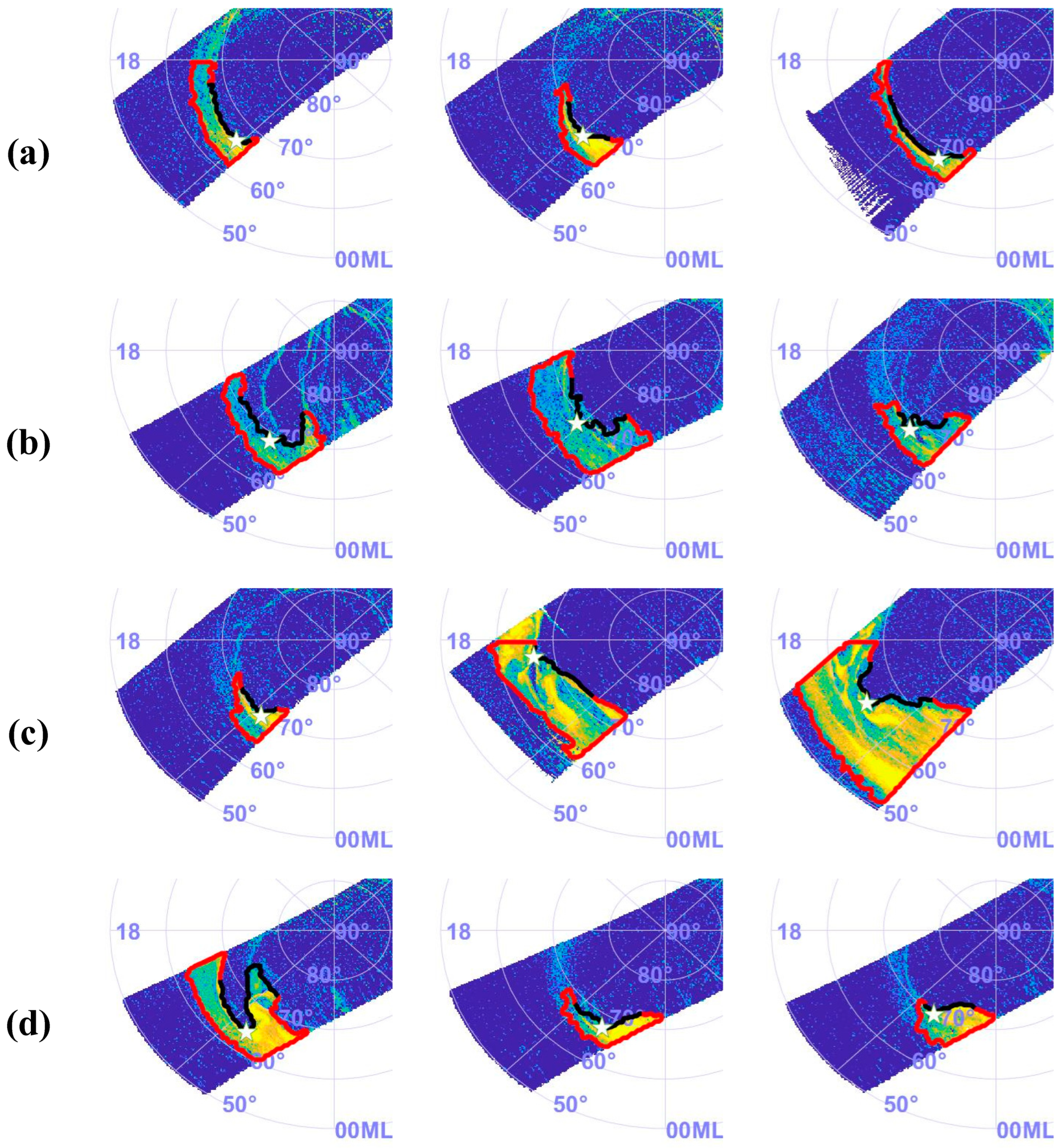
3.2.1. Analysis of Missed Events

In our experiments, the missed WTS events could be roughly divided into four categories, as shown in Figure 4.
Category 1 (Figure 4a): The WTS was in the initial stage, with no boundary position and intensity changes. Moreover, due to reasons such as satellite orbits, the WTS was not completely photographed, so the classifier only relied on the local image and could not extract the complete features of the WTS, which led to these events being missed.
Category 2 (Figure 4b): The selection of the WTS events were affected by human subjective factors and some events were identified as ambiguous. These cases, shown in Figure 4b, may or may not have contained a WTS. Therefore, it was difficult to judge whether it contained a WTS only by image, which led to missed identifications.
Category 3 (Figure 4c): When the WTS event had no obvious boundary features, it was impossible to identify whether the event contained a WTS only by the brightness intensification. The WTS event had no obvious western steep boundary or the WTS event was in the disappearance phase, but it could still be regarded as a WTS event.
Category 4 (Figure 4d): These cases included a WTS but they were missed. The main reason for the missed identification was that the WTS was large and the boundary features and intensity features extracted by the classifier were quite different from the feature distributions learned during training, which led to the classifier not identifying the WTS event.

3.2.2. Analysis of False-Alarm Events

The false-alarm events could also be divided into four categories, as shown in Figure 5.
Category 1 (Figure 5a): The polar boundary of an auroral oval is complex and without specific behavior patterns. As the intensity of the aurora data of SSUSI in the non-aurora region was zero, it was not necessary to locate the aurora region with a complex algorithm. A simple morphological processing approach was used to locate the boundary position of the auroral oval, which could be mistaken for the fold characteristic of the WTS, resulting in a false identification.
Category 2 (Figure 5b): The identification of a WTS is based on two factors: boundary features and brightness features. The brightness features were satisfied in these events, as shown in Figure 5b. Therefore, the intensity enhancement of the polar boundary of the aurora oval was mistaken for the PBI features of the WTS, resulting in a false identification.
Category 3 (Figure 5c): In these cases, there were extremely steep poleward boundaries in the auroral oval, but these features were not the boundary features of the WTS, which led to false identification.
To sum up, whether it was missed detection or a false-alarm, the main reason was that the description of the characteristics of the WTS was not accurate enough. Further improvement is needed on the existing characteristic descriptions.

4. Conclusions

In this paper, a new substorm identification approach was proposed for existing auroral data, which were mostly of low temporal resolution and high spatial resolution, to identify substorms by detecting the WTS. According to the static characteristic of a WTS, we defined a set of morphological-based feature parameters and designed a set of automatic detection and discrimination approaches. We used the extracted features and pattern recognition approach (SVM) to identify the WTS. This approach was tested using auroral data, which included 366 auroral images with a WTS and 533 auroral images without a WTS from the ultraviolet auroral spectral imager of the DMSP satellite. The results showed that the accuracy rate for the automatic identification of substorm and non-substorm events was 61.39%~63.61% and the precision rate of substorm identification was 55.52%~57.92%. Compared with previous approaches used to detect substorm events from UVI images, the precision of the proposed approach increased by about 7%. The experimental results showed that the approach in this paper was effective. In addition, the analysis results of under-reporting and false-reporting events indicated that improving the accuracy of the WTS feature description could effectively improve the accuracy and precision of substorm identification.
The definition of the static characteristic described in this paper was applied to the data obtained by the Ultraviolet Spectrographic Imager of the SMILE satellite program. The SMILE satellite can monitor the dynamic process of a substorm, so identification based on the static characteristic can be developed for identification based on the dynamic characteristic [36].

Author Contributions

Conceptualization, Z.-J.H., B.H. and Y.-S.Z.; approach, Z.-J.H., H.-F.L. and B.H.; software, H.-F.L. and B.-R.Z.; validation, Z.-J.H., H.-F.L., B.-R.Z., B.H. and Y.-S.Z.; formal analysis, Z.-J.H.; investigation, Z.-J.H.; resources, Z.-J.H.; data curation, Z.-J.H., H.-F.L. and B.-R.Z.; writing—original draft preparation, Z.-J.H., H.-F.L., B.-R.Z., B.H. and Y.-S.Z.; writing—review and editing, Z.-J.H.; visualization, H.-F.L. and B.-R.Z.; supervision, Z.-J.H.; project administration, Z.-J.H. and Y.-S.Z.; funding acquisition, Z.-J.H. and Y.-S.Z. All authors have read and agreed to the published version of the manuscript.

Funding

This research was funded by the National Natural Science Foundation of China (Grant Nos. 41831072, 41874195, and 42130210), the National Key R&D Program of China (Grant Nos. 2021YFE0106400 and 2018YFC1407303), the Space Science Pilot Project of the Chinese Academy of Sciences (grant number XDA15350202), a fund from the Institute of Applied Meteorology, and the Shanghai Pujiang Program.

Data Availability Statement

DMSP SSUSI data were provided by The Johns Hopkins University Applied Physics Laboratory (https://ssusi.jhuapl.edu/) (accessed on 30 August 2023).

Conflicts of Interest

The authors declare no conflict of interest.

References

  1. Xu, W. Energy Budget in the Coupling Processes of the Solar Wind, Magnetosphere and Ionosphere. Chin. J. Space Sci. 2011, 31, 1–14. (In Chinese) [Google Scholar] [CrossRef]
  2. Li, L.-Y.; Cao, J.-B.; Zhou, G.-C. Relation between the variation of geomagnetospheric relativistic electron flux and storm/substorm. Chin. J. Geophys. 2006, 49, 9–15. (In Chinese) [Google Scholar] [CrossRef]
  3. Yang, X.; Gao, X.B.; Song, B.; Yang, D. Aurora image search with contextual CNN feature. Neurocomputing 2018, 281, 67–77. [Google Scholar] [CrossRef]
  4. Wang, Q.-J.; Du, A.-M.; Zhao, X.-D.; Luo, H.; Xu, W.-Y. Manifestation of the AE index in substorms on 6 August 1998. Chin. J. Geophys. 2009, 52, 2943–2950. (In Chinese) [Google Scholar] [CrossRef]
  5. Sutcliffe, P.R. Substorm onset identification using neural networks and Pi2 pulsations. Ann. Geophys. 1997, 15, 1257–1264. [Google Scholar] [CrossRef]
  6. Murphy, K.R.; Rae, I.J.; Mann, I.R.; Milling, D.K.; Watt, C.E.J.; Ozeke, L.; Frey, H.U.; Angelopoulos, V.; Russell, C.T. Wavelet-based ULF wave diagnosis of substorm expansion phase onset. J. Geophys. Res. 2009, 114, A00C16. [Google Scholar] [CrossRef]
  7. Tokunaga, T.; Yumoto, K.; Uozumi, T.; CPMN Group. Identification of full-substorm onset from ground-magnetometer data by singular value transformation. Kyushu Univ. Ser. D Earth Planet. Sci. 2011, 32, 63–73. [Google Scholar] [CrossRef]
  8. Kataoka, R.; Miyoshi, Y.; Morioka, A. Hilbert-Huang Transform of geomagnetic pulsations at auroral expansion onset. J. Geophys. Res. Space Phys. 2009, 114, A09202. [Google Scholar] [CrossRef]
  9. Meng, C.I.; Kan, L. Substorm timings and timescales: A new aspect. Space Sci. Rev. 2004, 113, 41–75. [Google Scholar] [CrossRef]
  10. Hu, Z.; Yang, H.; Ai, Y.; Huang, D.; Hu, H.; Liu, R.; Taguchi, M.; Chen, Z.; Qi, X.; Wen, Y.; et al. Multiple wavelengths observation of dayside auroras in visible range—A preliminary result of the first wintering aurora observation in Chinese arctic station at Ny-Ålesund. Chin. J. Polar Res. 2005, 17, 107–114. (In Chinese) [Google Scholar]
  11. Hu, Z.-J.; Yang, H.; Huang, D.; Araki, T.; Sato, N.; Taguchi, M.; Seran, E.; Hu, H.; Liu, R.; Zhang, B.; et al. Synoptic distribution of dayside aurora: Multiple-wavelength all-sky observation at Yellow River Station in Ny-Ålesund, Svalbard. J. Atmos. Sol.-Terr. Phys. 2009, 71, 794–804. [Google Scholar] [CrossRef]
  12. Hu, Z.-J.; Yang, Q.-J.; Liang, J.-M.; Hu, H.Q.; Zhang, B.C.; Yang, H.G. Variation and modeling of ultraviolet auroral oval boundaries associated with interplanetary and geomagnetic parameters. Space Weather 2017, 15, 606–622. [Google Scholar] [CrossRef]
  13. Akasofu, S.I. The development of the auroral substorm. Planet. Space Sci. 1964, 12, 273–282. [Google Scholar] [CrossRef]
  14. Liou, K.; Meng, C.I.; Lui, T.Y.; Newell, P.T.; Brittnacher, M.; Parks, G.; Reeves, G.D.; Anderson, R.R.; Yumoto, K. On relative timing in substorm onset signatures. J. Geophys. Res. Space Phys. 1999, 104, 22807–22817. [Google Scholar] [CrossRef]
  15. Frey, H.U.; Mende, S.B.; Angelopoulos, V.; Donovan, E.F. Substorm onset observations by IMAGE-FUV. J. Geophys. Res. 2004, 109, A10304. [Google Scholar] [CrossRef]
  16. Liou, K. Polar Ultraviolet Imager observation of auroral breakup. J. Geophys. Res. 2010, 115, A12219. [Google Scholar] [CrossRef]
  17. Yang, Q.-J.; Liang, J.-M.; Liu, J.-M.; Hu, Z.-J.; Hu, H.-Q. A approach for automatic identification of substorm expansion phase onset from UVI images. Chin. J. Geophys. 2013, 56, 1435–1447. (In Chinese) [Google Scholar] [CrossRef]
  18. Akasofu, S.I.; Kimball, D.S.; Meng, C.I. The dynamics of the aurora—II Westward traveling surges. J. Atmos. Terr. Phys. 1965, 27, 173–187. [Google Scholar] [CrossRef]
  19. Ma, Y.Z.; Zhang, Q.H.; Lyons, L.R.; Liu, J.; Xing, Z.Y.; Reimer, A.; Nishimura, Y.; Hampton, D. Is westward travelling surge driven by the polar cap flow channels? J. Geophys. Res. Space Phys. 2021, 126, e2020JA028407. [Google Scholar] [CrossRef]
  20. Mcpherron, R.L. Growth phase of magnetospheric substorms. J. Geophys. Res. 1970, 75, 5592–5599. [Google Scholar] [CrossRef]
  21. Mcpherron, R.L. Substorm related changes in the geomagnetic tail: The growth phase. Planet. Space Sci. 1972, 20, 1521–1539. [Google Scholar] [CrossRef]
  22. Samson, J.C.; Rostoker, G. Polarization characteristic of Pi 2 pulsations and implications for their source mechanisms: Influence of the westward travelling surge. Planet. Space Sci. 1983, 31, 435–458. [Google Scholar] [CrossRef]
  23. Lyons, L.R.; Nagai, T.; Blanchard, G.T.; Samson, J.C.; Yamamoto, T.; Mukai, T.; Nishida, A.; Kokubun, S. Association between Geotail plasma flows and auroral poleward boundary intensifications observed by CANOPUS photometers. J. Geophys. Res. 1999, 104, 4485–4500. [Google Scholar] [CrossRef]
  24. Sergeev, V.A.; Sauvaud, J.A.; Popescu, D.; Kovrazhkin, R.A.; Liou, K.; Newell, P.T.; Brittnacher, M.; Parks, G.; Nakamura, R.; Mukai, T.; et al. Multiple-spacecraft observation of a narrow transient plasma jet in the Earth’s plasma sheet. Geophys. Res. Lett. 2000, 27, 851–854. [Google Scholar] [CrossRef]
  25. Nakamura, R.; Baumjohann, W.; Schödel, R.; Brittnacher, M.; Sergeev, V.A.; Kubyshkina, M.; Mukai, T.; Liou, K. Earthward flow bursts, auroral streamers, and small expansions. J. Geophys. Res. 2001, 106, 10791–10802. [Google Scholar] [CrossRef]
  26. Nishimura, Y.; Lyons, L.R.; Angelopoulos, V.; Kikuchi, T.; Zou, S.; Mende, S.B. Relations between multiple auroral streamers, pre-onset thin arc formation, and substorm auroral onset. J. Geophys. Res. 2011, 116, A09214. [Google Scholar] [CrossRef]
  27. Hardy, D.A.; Schmitt, L.K.; Gussenhoven, M.S.; Marshall, F.J.; Yeh, H.C. Precipitating electron and ion detectors (SSJ/4) for the block 5D/flights 6–10 DMSP (Defense Meteorological Satellite Program) satellites: Calibration and data presentation. Rep. Air Force Geophys. Lab. 1984. Hanscom Air Force Base, Bedford, Mass. [Google Scholar]
  28. Morrison, D.; Paxton, L.J.; Humm, D.C. On-orbit calibration of the Special Sensor Ultraviolet Scanning Imager (SSUSI): A far-UV imaging spectrograph on DMSP F-16. Proc. SPIE-Int. Soc. Opt. Eng. 2022, 4485, 328–337. [Google Scholar] [CrossRef]
  29. Paxton, L.J.; Morrison, D.; Zhang, Y.; Kil, H.; Wolven, B.; Ogorzalek, B.S.; Humm, D.C.; Meng, C.I. Validation of remote sensing products produced by the special sensor ultraviolet scanning imager (SSUSI): A far UV imaging spectrograph on DMSP F-16. In Proceedings of the Proc. SPIE 4485, Optical Spectroscopic Techniques, Remote Sensing, and Instrumentation for Atmospheric and Space Research IV, San Diego, CA, USA, 30 January 2002. [Google Scholar] [CrossRef]
  30. Hu, Z.J.; Han, B.; Lian, H.-F.; Zhao, B.-R. SSUSI Images Acquired by Ultraviolet Spectrographic Imager Aboard DMSP Satellite from October to December during 2004–2006 [Data Set]. Zenodo 2023. [Google Scholar] [CrossRef]
  31. Wang, Q.; Meng, Q.H.; Hu, Z.J.; Xing, Z.Y.; Liang, J.M.; Hu, H.Q. Extraction of Auroral Oval Boundaries from Uvi Images: A New Flicm Clustering-Based Approach and Its Evaluation. Adv. Polar Sci. 2011, 22, 184–191. Available online: https://aps.chinare.org.cn/EN/10.3724/SP.J.1085.2011.00184 (accessed on 30 August 2023).
  32. Wang, Q.; Meng, Q.H.; Hu, Z.J.; Xing, Z.Y.; Liang, J.M.; Hu, H.Q. A approach for extracting auroral ovals in UVI images and its evaluation. Chin. J. Polar Res. 2011, 23, 168–177. (In Chinese) [Google Scholar]
  33. Yang, Q.J.; Hu, Z.J.; Han, D.S.; Hu, H.Q.; Ma, X. Modeling and prediction of ultraviolet auroral oval boundaries based on IMF/solar wind and geomagnetic parameters. Chin. J. Geophys. 2016, 59, 426–439. (In Chinese) [Google Scholar] [CrossRef]
  34. Han, B.; Lian, H.F.; Hu, Z.J. Modeling of ultraviolet auroral oval boundaries based on neural network technology. Sci. Sin. Technol. 2019, 49, 531–542. [Google Scholar] [CrossRef]
  35. Vapnik, V.N. Statistical Learning Theory; Wiley: New York, NY, USA, 1998. [Google Scholar]
  36. Wang, C.; Graziella, B.R. Progress of Solar Wind Magnetosphere Ionosphere Link Explorer (SMILE) Mission. Chin. J. Space Sci. 2018, 38, 657–661. [Google Scholar] [CrossRef]
Figure 1. (Left) ultraviolet (UV) auroral image from SSUSI of DMSP F16 with the altitude-adjusted corrected geomagnetic (AACGM) coordinates; (right) auroral oval fragment from 18–24 MLT sectors from the left UV image.
Universe 09 00412 g001
Figure 2. Region of WTS and the extreme value point (the white asterisk).
Universe 09 00412 g002
Figure 3. The process of the WTS recognition.
Universe 09 00412 g003
Figure 4. Example diagram of missed WTS events.
Universe 09 00412 g004
Figure 5. Example diagram of false-alarm events.
Universe 09 00412 g005
Table 1. Confusion matrix with train–test ratio of 1:9.
Train–Test RatioTrue CategoriesSVM Classifier Determination CategoriesTotal
WTSNo WTS
1:9WTSa = 162b = 165327
No WTSc = 131d = 341472
Total293506799
Table 2. The five indicators for different train–test ratios.
Train–Test RatioRaccuracyRrecallRmissRfalse-alarmRprecision
1:963.00%49.66%50.34%44.48%55.52%
2:863.61%41.24%58.77%42.08%57.92%
3:762.73%40.94%59.06%43.40%56.60%
4:661.39%23.95%76.05%42.97%57.03%
5:562.22%31.46%68.55%42.40%57.60%
Disclaimer/Publisher’s Note: The statements, opinions and data contained in all publications are solely those of the individual author(s) and contributor(s) and not of MDPI and/or the editor(s). MDPI and/or the editor(s) disclaim responsibility for any injury to people or property resulting from any ideas, methods, instructions or products referred to in the content.

