
Comparative Study of Dayside Pulsating Auroras Induced by Ultralow-Frequency Waves

 , , , , , , , , , , , , and
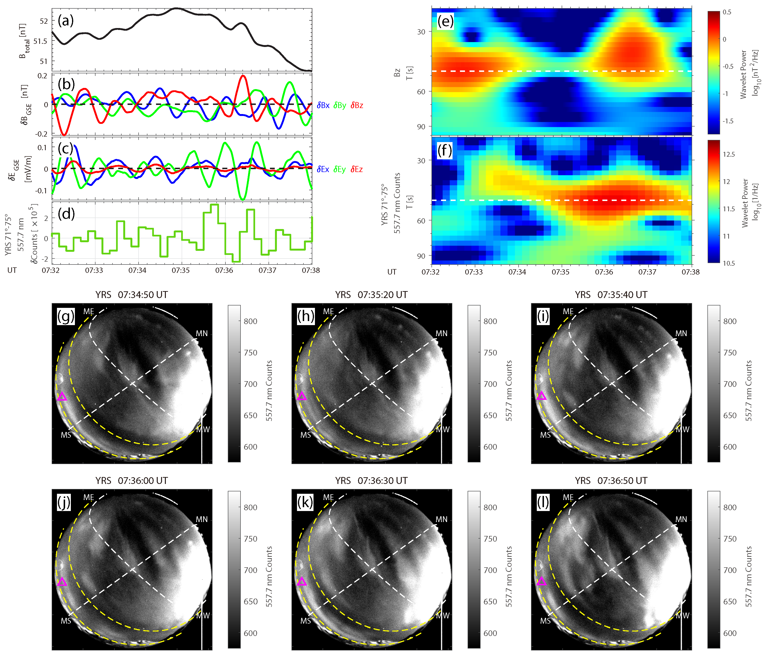
Abstract
:1. Introduction
2. Instrumentation and Methods
3. Results
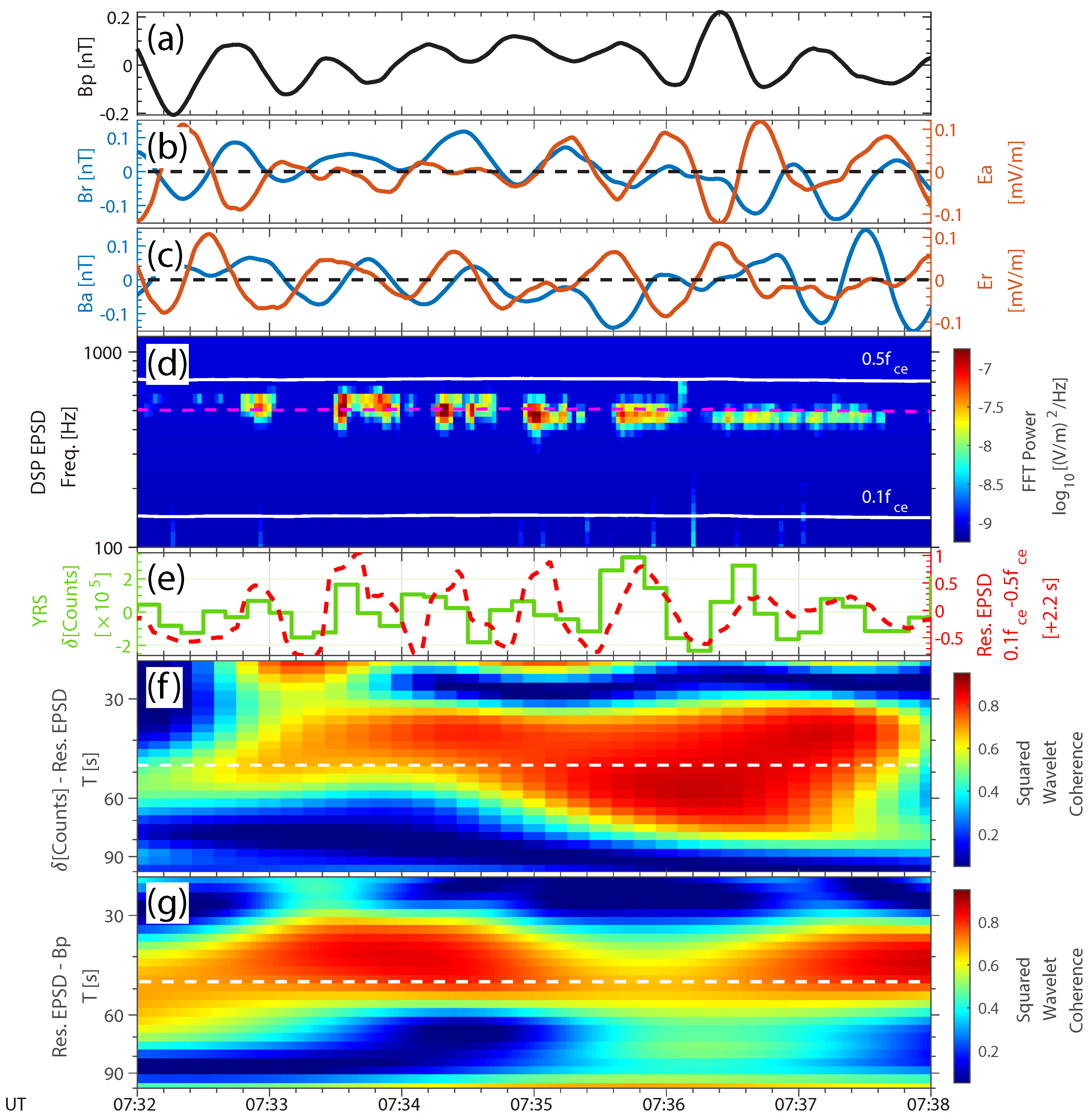
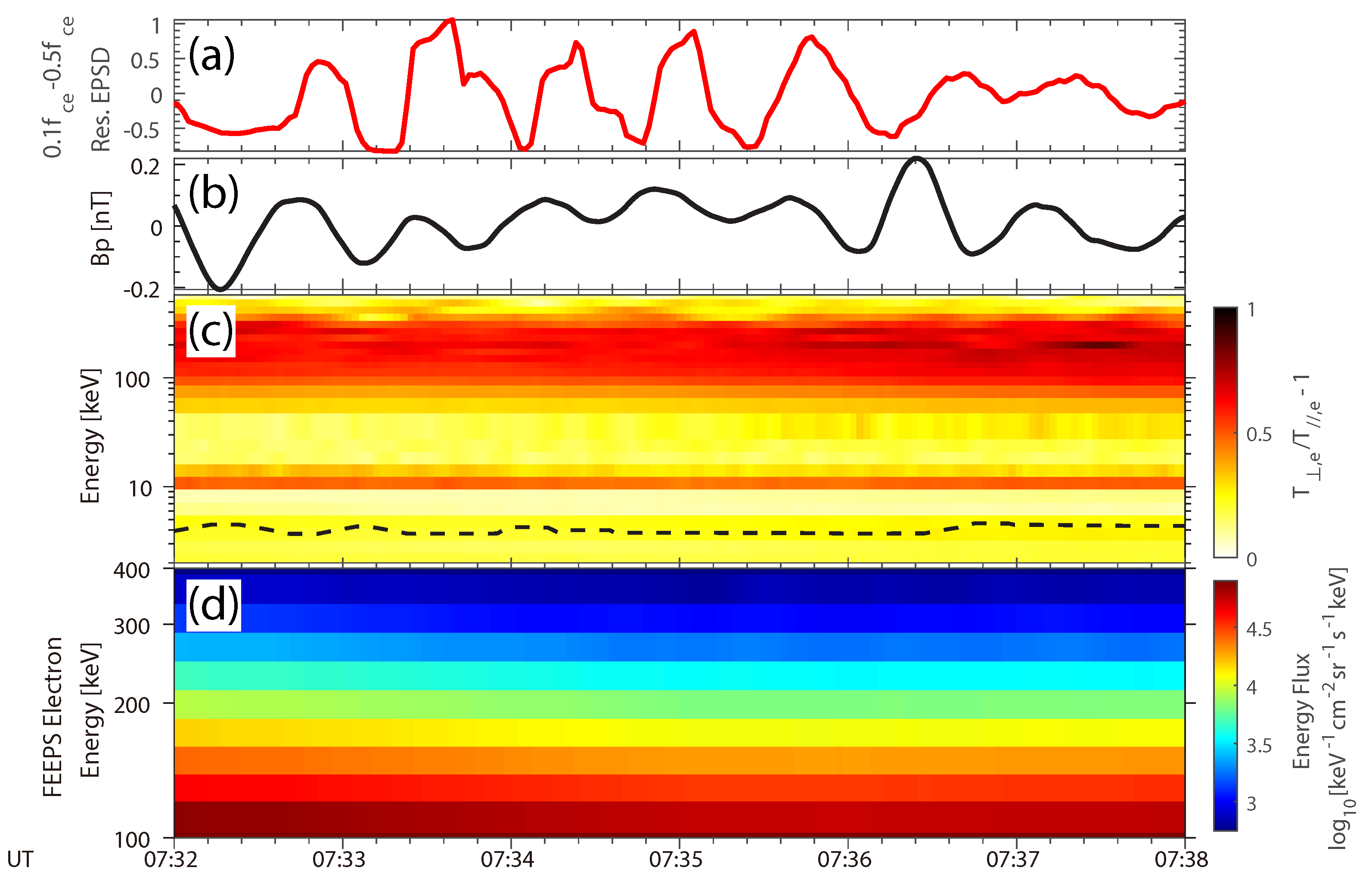
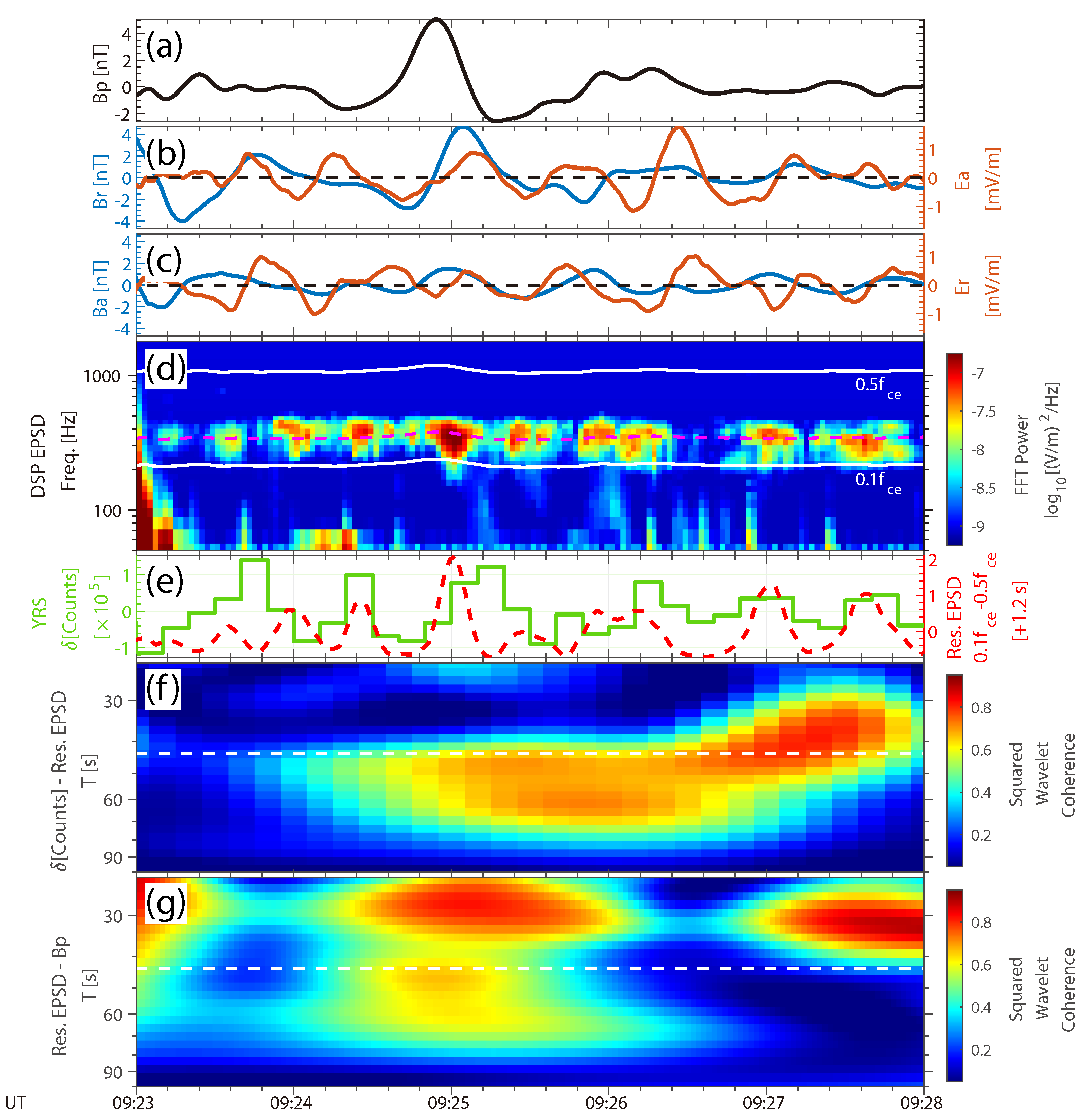
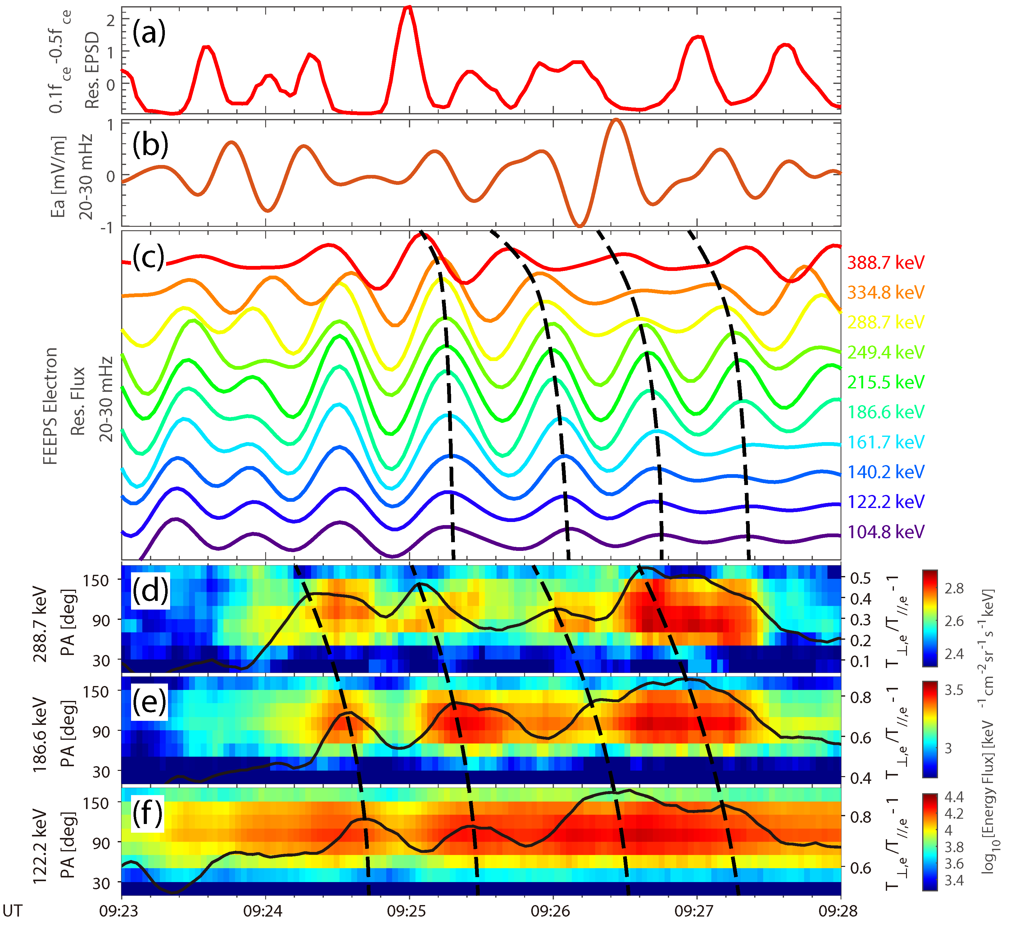
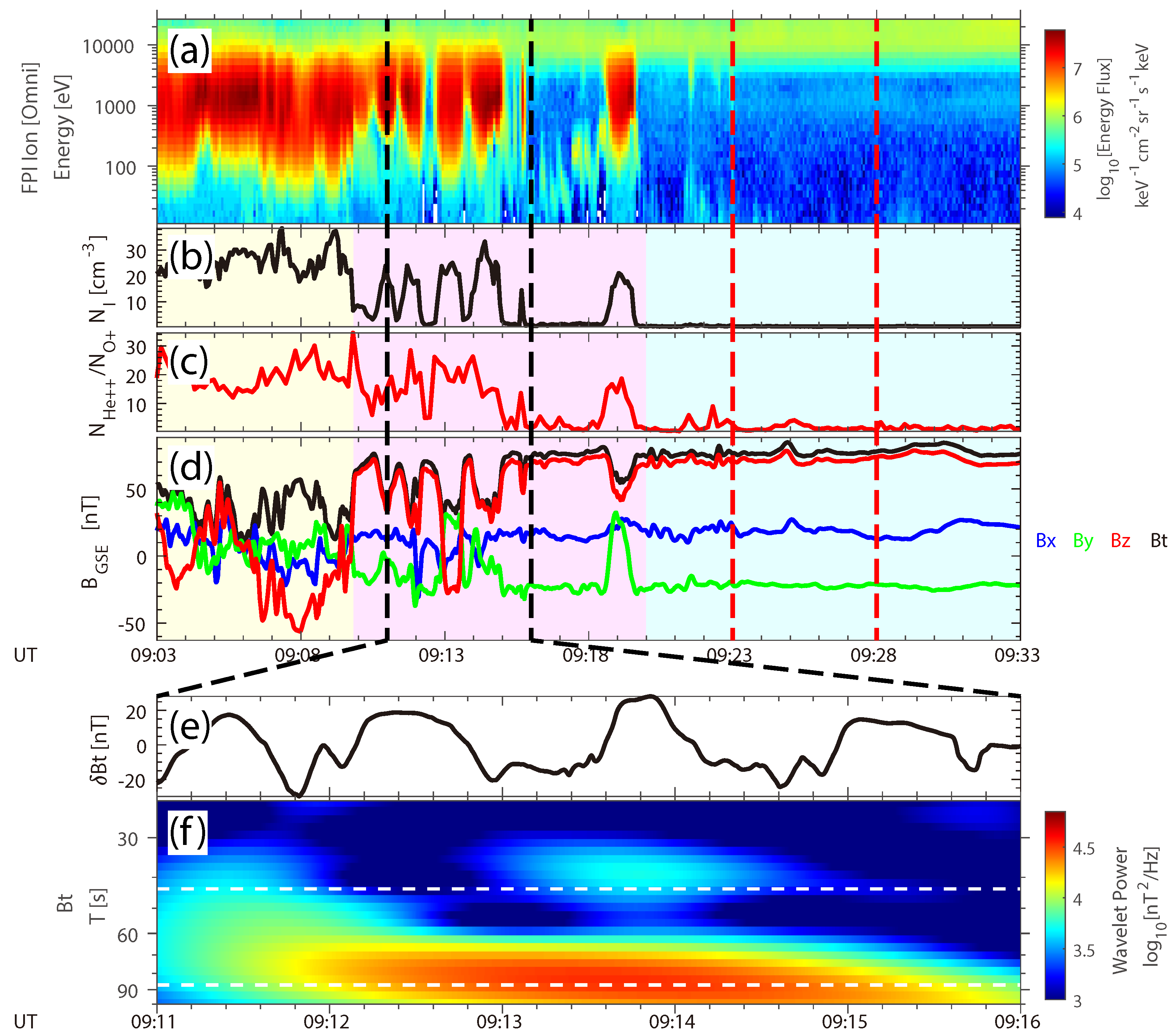
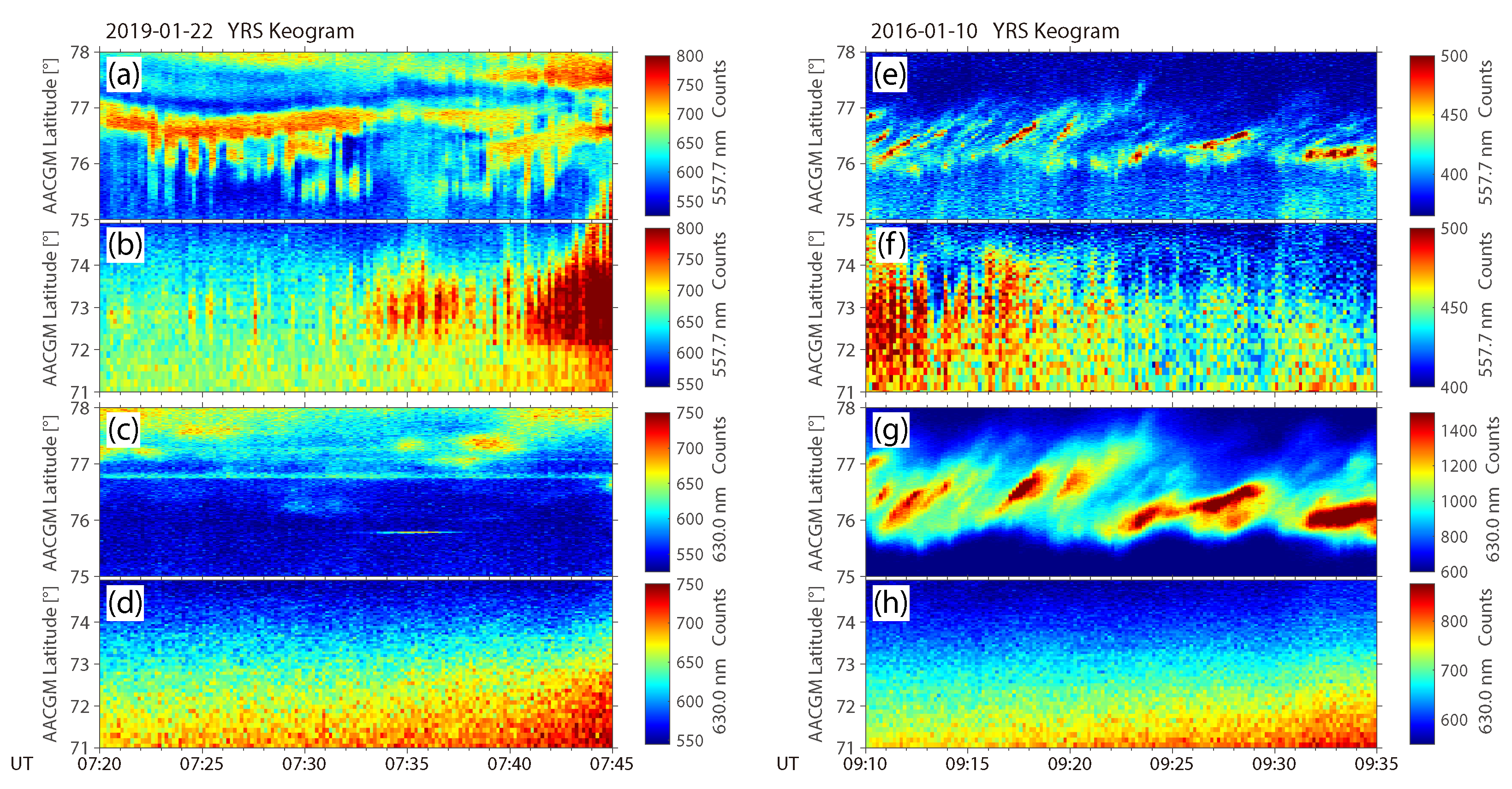
3.1. The 22 January 2019 Event
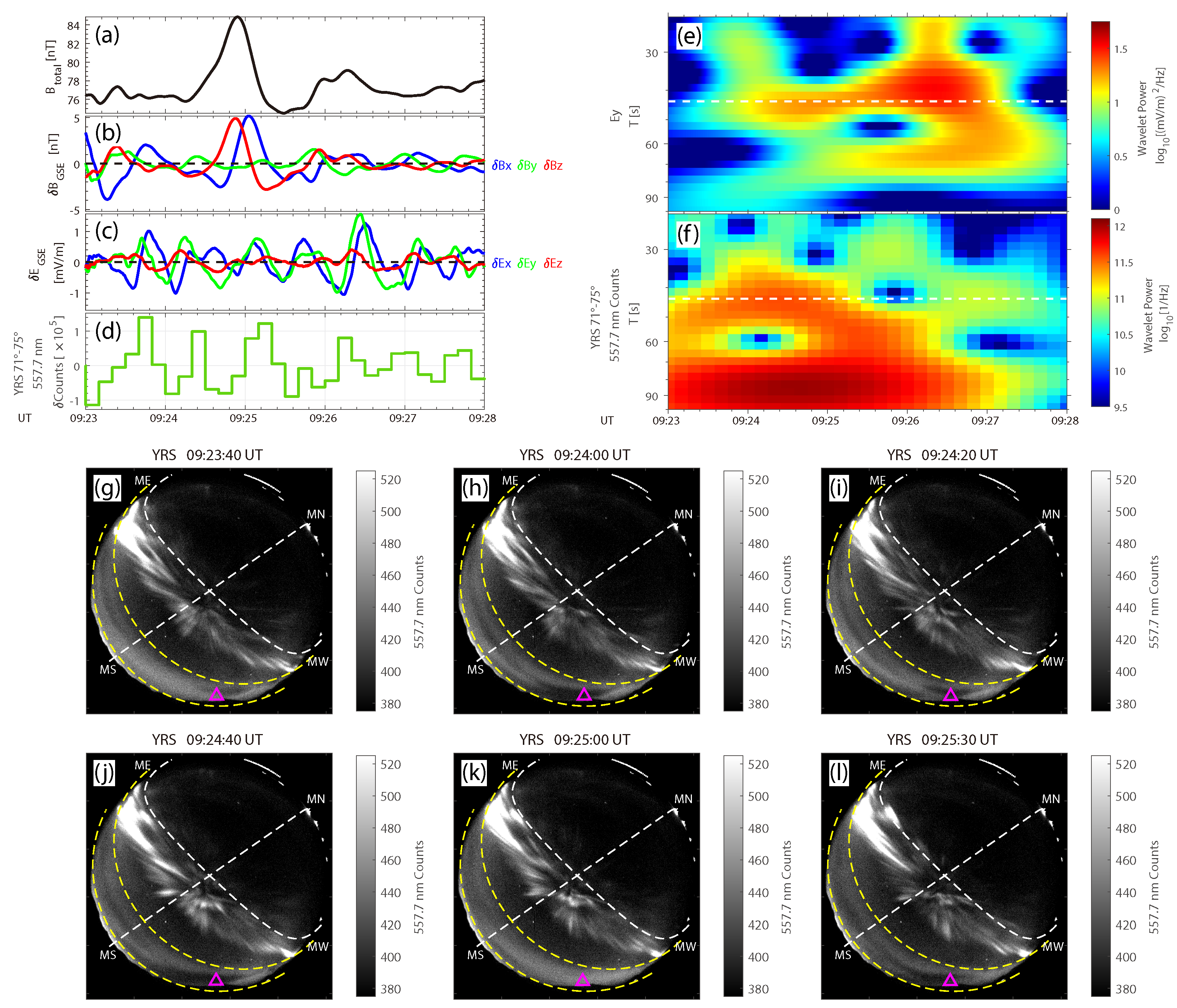
3.2. The 10 January 2016 Event
4. Discussion
- In Event 1, we observed that the frequencies of auroral pulsations and compressional ULF waves are similar to each other, whereas in Event 2, the oscillation period of auroral pulsations is close to that of transverse ULF waves.
- We identified that the modulation of chorus waves in Event 1 is caused by the change in the threshold for the whistler anisotropy instability induced by ULF waves. However, in Event 2, the modulation results from the variation of electron temperature anisotropy generated by ULF waves.
- Our analysis suggests that the relatively low coherence between chorus intensity and ULF wave fields in Event 2 may be attributed to phase shifts induced by drift resonance.
Supplementary Materials
Author Contributions
Funding
Data Availability Statement
Acknowledgments
Conflicts of Interest
References
- Zong, Q.G.; Rankin, R.; Zhou, X.Z. The interaction of ultralow-frequency pc3-5 waves with charged particles in Earth’s magnetosphere. Rev. Mod. Plasma Phys. 2017, 1, 10. [Google Scholar] [CrossRef]
- Jacobs, J.; Kato, Y.; Matsushita, S.; Troitskaya, V. Classification of geomagnetic micropulsations. J. Geophys. Res. 1964, 69, 180–181. [Google Scholar] [CrossRef]
- Samson, J.C.; Jacobs, J.A.; Rostoker, G. Latitude-dependent characteristics of long-period geomagnetic micropulsations. J. Geophys. Res. 1971, 76, 3675–3683. [Google Scholar] [CrossRef]
- Claudepierre, S.G.; Elkington, S.R.; Wiltberger, M. Solar wind driving of magnetospheric ULF waves: Pulsations driven by velocity shear at the magnetopause. J. Geophys. Res. 2008, 113, A05218. [Google Scholar] [CrossRef]
- Zong, Q.G.; Zhou, X.Z.; Wang, Y.F.; Li, X.; Song, P.; Baker, D.N.; Fritz, T.A.; Daly, P.W.; Dunlop, M.; Pedersen, A. Energetic electrons response to ULF waves induced by interplanetary shocks in the outer radiation belt. J. Geophys. Res. 2009, 114, A10204. [Google Scholar] [CrossRef]
- Liu, W.; Sarris, T.; Li, X.; Ergun, R.; Angelopoulos, V.; Bonnell, J.; Glassmeier, K. Solar wind influence on Pc4 and Pc5 ULF wave activity in the inner magnetosphere. J. Geophys. Res. 2010, 115, A12201. [Google Scholar] [CrossRef]
- Southwood, D.J.; Kivelson, M.G. Charged particle behavior in low-frequency geomagnetic pulsations. I—Transverse waves. J. Geophys. Res. 1981, 86, 5643–5655. [Google Scholar] [CrossRef]
- Southwood, D.J.; Kivelson, M.G. Charged particle behavior in low-frequency geomagnetic pulsations. II—Graphical approach. J. Geophys. Res. 1982, 87, 1707–1710. [Google Scholar] [CrossRef]
- Hao, Y.X.; Zong, Q.G.; Wang, Y.F.; Zhou, X.Z.; Zhang, H.; Fu, S.Y.; Pu, Z.Y.; Spence, H.E.; Blake, J.B.; Bonnell, J.; et al. Interactions of energetic electrons with ULF waves triggered by interplanetary shock: Van Allen Probes observations in the magnetotail. J. Geophys. Res. 2014, 119, 8262–8273. [Google Scholar] [CrossRef]
- Claudepierre, S.G.; Mann, I.R.; Takahashi, K.; Fennell, J.F.; Hudson, M.K.; Blake, J.B.; Roeder, J.L.; Clemmons, J.H.; Spence, H.E.; Reeves, G.D.; et al. Van Allen Probes observation of localized drift resonance between poloidal mode ultra-low frequency waves and 60 keV electrons. Geophys. Res. Lett. 2013, 40, 4491–4497. [Google Scholar] [CrossRef]
- Elkington, S.R.; Sarris, T.E. The role of pc-5 ULF waves in the radiation belts: Current understanding and open questions. In Waves, Particles, and Storms in Geospace: A Complex Interplay; Oxford University Press (OUP): Oxford, UK, 2016; p. 80. [Google Scholar]
- Li, L.; Zhou, X.Z.; Omura, Y.; Zong, Q.G.; Rankin, R.; Chen, X.R.; Liu, Y.; Yue, C.; Fu, S.Y. Drift resonance between particles and compressional toroidal ULF waves in dipole magnetic field. J. Geophys. Res. 2021, 126, e2020JA028842. [Google Scholar] [CrossRef]
- Oimatsu, S.; Nosé, M.; Teramoto, M.; Yamamoto, K.; Matsuoka, A.; Kasahara, S.; Yokota, S.; Keika, K.; Le, G.; Nomura, R.; et al. Drift-bounce resonance between pc5 pulsations and ions at multiple energies in the nightside magnetosphere: Arase and MMS observations. Geophys. Res. Lett. 2018, 45, 7277–7286. [Google Scholar] [CrossRef]
- Oimatsu, S.; Nosé, M.; Le, G.; Fuselier, S.A.; Ergun, R.E.; Lindqvist, P.; Sormakov, D. Selective acceleration of O+ by drift-bounce resonance in the Earth’s magnetosphere: MMS observations. J. Geophys. Res. 2020, 125, e2019JA027686. [Google Scholar] [CrossRef]
- Zong, Q.G.; Wang, Y.F.; Zhang, H.; Fu, S.Y.; Zhang, H.; Wang, C.R.; Yuan, C.J.; Vogiatzis, I. Fast acceleration of inner magnetospheric hydrogen and oxygen ions by shock induced ULF waves. J. Geophys. Res. 2012, 117, A11206. [Google Scholar] [CrossRef]
- Min, K.; Takahashi, K.; Ukhorskiy, A.Y.; Manweiler, J.W.; Spence, H.E.; Singer, H.J.; Claudepierre, S.G.; Larsen, B.A.; Soto-Chavez, A.R.; Cohen, R.J. Second harmonic poloidal waves observed by Van Allen Probes in the dusk-midnight sector. J. Geophys. Res. 2017, 122, 3013–3039. [Google Scholar] [CrossRef]
- Yamamoto, K.; Nosé, M.; Keika, K.; Hartley, D.P.; Smith, C.W.; MacDowall, R.J.; Lanzerotti, L.J.; Mitchell, D.G.; Spence, H.E.; Reeves, G.D.; et al. Eastward propagating second harmonic poloidal waves triggered by temporary outward gradient of proton phase space density: Van Allen Probe A observation. J. Geophys. Res. 2019, 124, 9904–9923. [Google Scholar] [CrossRef]
- Liu, Z.Y.; Zong, Q.G.; Zhou, X.Z.; Zhu, Y.F.; Gu, S.J. Pitch Angle Structures of Ring Current Ions Induced by Evolving Poloidal Ultra-Low Frequency Waves. Geophys. Res. Lett. 2020, 47, e2020GL087203. [Google Scholar] [CrossRef]
- Li, X.Y.; Liu, Z.Y.; Zong, Q.G.; Zhou, X.Z.; Hao, Y.X.; Rankin, R.; Zhang, X.X. Pitch angle phase shift in ring current ions interacting with ultra-low-frequency waves: Van Allen Probes observations. J. Geophys. Res. 2021, 126, e2020JA029025. [Google Scholar] [CrossRef]
- Liu, Z.Y.; Zong, Q.G.; Rankin, R.; Zhang, H.; Wang, Y.F.; Zhou, X.Z.; Fu, S.Y.; Yue, C.; Zhu, X.Y.; Pollock, C.J.; et al. Simultaneous macroscale and microscale wave-ion interaction in near-earth space plasmas. Nat. Commun. 2022, 13, 5593. [Google Scholar] [CrossRef]
- Li, W.; Thorne, R.; Bortnik, J.; Nishimura, Y.; Angelopoulos, V. Modulation of whistler mode chorus waves: 1. Role of compressional Pc4-5 pulsations. J. Geophys. Res. 2011, 116, A06206. [Google Scholar] [CrossRef]
- Xia, Z.; Chen, L.; Dai, L.; Claudepierre, S.G.; Chan, A.A.; Soto-Chavez, A.R.; Reeves, G.D. Modulation of chorus intensity by ULF waves deep in the inner magnetosphere. Geophys. Res. Lett. 2016, 43, 9444–9452. [Google Scholar] [CrossRef]
- Zhang, X.J.; Chen, L.; Artemyev, A.V.; Angelopoulos, V.; Liu, X. Periodic excitation of chorus and ECH waves modulated by ultralow frequency compressions. J. Geophys. Res. 2019, 124, 8535–8550. [Google Scholar] [CrossRef]
- Zhang, X.J.; Angelopoulos, V.; Artemyev, A.V.; Hartinger, M.D.; Bortnik, J. Modulation of whistler waves by ultra-low-frequency perturbations: The importance of magnetopause location. J. Geophys. Res. 2020, 125, e2020JA028334. [Google Scholar] [CrossRef]
- Li, L.; Omura, Y.; Zhou, X.Z.; Zong, Q.G.; Rankin, R.; Yue, C.; Fu, S.Y. Nonlinear wave growth analysis of chorus emissions modulated by ULF waves. Geophys. Res. Lett. 2022, 49, e2022GL097978. [Google Scholar] [CrossRef]
- Thorne, R.M.; Ni, B.; Tao, X.; Horne, R.B.; Meredith, N.P. Scattering by chorus waves as the dominant cause of diffuse auroral precipitation. Nature 2010, 467, 943–946. [Google Scholar] [CrossRef]
- Shi, R.; Hu, Z.J.; Ni, B.; Han, D.; Chen, X.C.; Zhou, C.; Gu, X. Modulation of the dayside diffuse auroral intensity by the solar wind dynamic pressure. J. Geophys. Res. 2014, 119, 10092–10099. [Google Scholar] [CrossRef]
- Ni, B.; Thorne, R.M.; Zhang, X.; Bortnik, J.; Pu, Z.; Xie, L.; Hu, Z.J.; Han, D.; Shi, R.; Zhou, C.; et al. Origins of the earth’s diffuse auroral precipitation. Space Sci. Rev. 2016, 200, 205–259. [Google Scholar] [CrossRef]
- Fukizawa, M.; Sakanoi, T.; Miyoshi, Y.; Hosokawa, K.; Shiokawa, K.; Katoh, Y.; Kazama, Y.; Kumamoto, A.; Tsuchiya, F.; Miyashita, Y.; et al. Electrostatic electron cyclotron harmonic waves as a candidate to cause pulsating auroras. Geophys. Res. Lett. 2018, 45, 12661–12668. [Google Scholar] [CrossRef]
- Kasahara, S.; Miyoshi, Y.; Yokota, S.; Mitani, T.; Kasahara, Y.; Matsuda, S.; Kumamoto, A.; Matsuoka, A.; Kazama, Y.; Frey, H.U.; et al. Pulsating aurora from electron scattering by chorus waves. Nature 2018, 554, 337–340. [Google Scholar] [CrossRef]
- Hosokawa, K.; Miyoshi, Y.; Ozaki, M.; Oyama, S.I.; Ogawa, Y.; Kurita, S.; Kasahara, Y.; Kasaba, Y.; Yagitani, S.; Matsuda, S.; et al. Multiple time-scale beats in aurora: Precise orchestration via magnetospheric chorus waves. Sci. Rep. 2020, 10, 3380. [Google Scholar] [CrossRef]
- Motoba, T.; Ebihara, Y.; Ogawa, Y.; Kadokura, A.; Engebretson, M.J.; Angelopoulos, V.; Gerrard, A.J.; Weatherwax, A.T. On the driver of daytime Pc3 auroral pulsations. Geophys. Res. Lett. 2019, 46, 553–561. [Google Scholar] [CrossRef]
- Motoba, T.; Ogawa, Y.; Ebihara, Y.; Kadokura, A.; Gerrard, A.J.; Weatherwax, A.T. Daytime Pc5 diffuse auroral pulsations and their association with outer magnetospheric ULF waves. J. Geophys. Res. 2021, 126, e2021JA029218. [Google Scholar] [CrossRef]
- Burch, J.L.; Moore, T.E.; Torbert, R.B.; Giles, B.L. Magnetospheric Multiscale overview and science objectives. Space Sci. Rev. 2016, 199, 5–21. [Google Scholar] [CrossRef]
- Blake, J.B.; Mauk, B.H.; Baker, D.N.; Carranza, P.; Clemmons, J.H.; Craft, J.; Crain, J.W., Jr.; Crew, A.; Dotan, Y.; Fennell, J.F.; et al. The Fly’s Eye Energetic Particle Spectrometer (FEEPS) sensors for the Magnetospheric Multiscale (MMS) mission. Space Sci. Rev. 2016, 199, 309–329. [Google Scholar] [CrossRef]
- Pollock, C.; Moore, T.; Jacques, A.; Burch, J.; Gliese, U.; Saito, Y.; Omoto, T.; Avanov, L.; Barrie, A.; Coffey, V.; et al. Fast Plasma Investigation for Magnetospheric Multiscale. Space Sci. Rev. 2016, 199, 331–406. [Google Scholar] [CrossRef]
- Young, D.T.; Burch, J.L.; Gomez, R.G.; Santos, A.D.L.; Miller, G.P.; IV, P.W.; Paschalidis, N.; Fuselier, S.A.; Pickens, K.; Hertzberg, E.; et al. Hot plasma composition analyzer for the Magnetospheric Multiscale mission. Space Sci. Rev. 2016, 199, 407–470. [Google Scholar] [CrossRef]
- Russell, C.T.; Anderson, B.J.; Baumjohann, W.; Bromund, K.R.; Dearborn, D.; Fischer, D.; Le, G.; Leinweber, H.K.; Leneman, D.; Magnes, W.; et al. The Magnetospheric Multiscale magnetometers. Space Sci. Rev. 2016, 199, 189–256. [Google Scholar] [CrossRef]
- Ergun, R.E.; Tucker, S.; Westfall, J.; Goodrich, K.A.; Malaspina, D.M.; Summers, D.; Wallace, J.; Karlsson, M.; Mack, J.; Brennan, N.; et al. The axial double probe and fields signal processing for the MMS mission. Space Sci. Rev. 2016, 199, 167–188. [Google Scholar] [CrossRef]
- Lindqvist, P.A.; Olsson, G.; Torbert, R.B.; King, B.; Granoff, M.; Rau, D.; Needell, G.; Turco, S.; Dors, I.; Beckman, P.; et al. The spin-plane double probe electric field instrument for MMS. Space Sci. Rev. 2016, 199, 137–165. [Google Scholar] [CrossRef]
- Torbert, R.B.; Russell, C.T.; Magnes, W.; Ergun, R.E.; Lindqvist, P.A.; LeContel, O.; Vaith, H.; Macri, J.; Myers, S.; Rau, D.; et al. The FIELDS instrument suite on MMS: Scientific objectives, measurements, and data products. Space Sci. Rev. 2016, 199, 105–135. [Google Scholar] [CrossRef]
- Hu, Z.J.; Yang, H.; Huang, D.; Araki, T.; Sato, N.; Taguchi, M.; Seran, E.; Hu, H.; Liu, R.; Zhang, B.; et al. Synoptic distribution of dayside aurora: Multiple-wavelength all-sky observation at Yellow River Station in Ny-Ålesund, Svalbard. J. Atmos. Sol.-Terr. Phys. 2009, 71, 794–804. [Google Scholar] [CrossRef]
- Tsyganenko, N.A. A model of the near magnetosphere with a dawn-dusk asymmetry 1. Mathematical structure. J. Geophys. Res. 2002, 107, SMP 12-1–SMP 12-15. [Google Scholar] [CrossRef]
- Tsyganenko, N.A. A model of the near magnetosphere with a dawn-dusk asymmetry 2. Parameterization and fitting to observations. J. Geophys. Res. 2002, 107, SMP 10-1–SMP 10-17. [Google Scholar] [CrossRef]
- Grinsted, A.; Moore, J.; Jevrejeva, S. Application of the cross wavelet transform and wavelet coherence to geophysical time series. Nonlinear Process. Geophys. 2004, 11, 561–566. [Google Scholar] [CrossRef]
- Kennel, C.F.; Petschek, H.E. Limit on stably trapped particle fluxes. J. Geophys. Res. 1966, 71, 1–28. [Google Scholar] [CrossRef]
- Hamlin, D.A.; Karplus, R.; Vik, R.C.; Watson, K.M. Mirror and azimuthal drift frequencies for geomagnetically trapped particles. J. Geophys. Res. 1961, 66, 1–4. [Google Scholar] [CrossRef]
- Gary, S.P.; Wang, J. Whistler instability: Electron anisotropy upper bound. J. Geophys. Res. 1996, 101, 10749–10754. [Google Scholar] [CrossRef]
- Fu, H.; Yue, C.; Ma, Q.; Kang, N.; Bortnik, J.; Zong, Q.G.; Zhou, X.Z. Frequency-dependent responses of plasmaspheric hiss to the impact of an interplanetary shock. Geophys. Res. Lett. 2021, 48, e2021GL094810. [Google Scholar] [CrossRef]
- Zhang, H.; Zong, Q.; Connor, H.; Delamere, P.; Facskó, G.; Han, D.; Hasegawa, H.; Kallio, E.; Kis, Á.; Le, G.; et al. Dayside transient phenomena and their impact on the magnetosphere and ionosphere. Space Sci. Rev. 2022, 218, 40. [Google Scholar] [CrossRef]
- Wang, B.; Nishimura, Y.; Hietala, H.; Angelopoulos, V. Investigating the role of magnetosheath high-speed jets in triggering dayside ground magnetic ultra-low frequency waves. Geophys. Res. Lett. 2022, 49, e2022GL099768. [Google Scholar] [CrossRef]
- Bolshakova, O.V.; Troitskaya, V.A. Relation of the IMF direction to the system of stable oscillations. Dokl. Akad. Nauk. USSR 1968, 180, 343–346. [Google Scholar]
- Troitskaya, V.A. Discoveries of sources of Pc 2-4 waves-A review of research in the former USSR. In Solar Wind Sources of Magnetospheric Ultra-Low-Frequency Waves; Engebretson, M.J., Takahashi, K., Scholer, M., Eds.; American Geophysical Union (AGU): Washington, DC, USA, 1994; pp. 45–54. [Google Scholar] [CrossRef]
- Heilig, B.; Lühr, H.; Rother, M. Comprehensive study of ULF upstream waves observed in the topside ionosphere by CHAMP and on the ground. Ann. Geophys. 2007, 25, 737–754. [Google Scholar] [CrossRef]
- Bier, E.A.; Owusu, N.; Engebretson, M.J.; Posch, J.L.; Lessard, M.R.; Pilipenko, V.A. Investigating the IMF cone angle control of Pc3-4 pulsations observed on the ground. J. Geophys. Res. 2014, 119, 1797–1813. [Google Scholar] [CrossRef]
- Glassmeier, K.H.; Auster, H.U.; Constantinescu, D.; Fornaçon, K.H.; Narita, Y.; Plaschke, F.; Angelopoulos, V.; Georgescu, E.; Baumjohann, W.; Magnes, W.; et al. Magnetospheric quasi-static response to the dynamic magnetosheath: A THEMIS case study. Geophys. Res. Lett. 2008, 35, L17S01. [Google Scholar] [CrossRef]
- Southwood, D.J. Some features of field line resonances in the magnetosphere. Planet. Space Sci. 1974, 22, 483–491. [Google Scholar] [CrossRef]
- Rae, I.J.; Donovan, E.F.; Mann, I.R.; Fenrich, F.R.; Watt, C.E.J.; Milling, D.K.; Lester, M.; Lavraud, B.; Wild, J.A.; Singer, H.J.; et al. Evolution and characteristics of global Pc5 ULF waves during a high solar wind speed interval. J. Geophys. Res. 2005, 110, A12211. [Google Scholar] [CrossRef]
- Shabansky, V.P. Some processes in the magnetosphere. Space Sci. Rev. 1971, 12, 299–418. [Google Scholar] [CrossRef]
- Li, X.Y.; Liu, Z.Y.; Zong, Q.G.; Zhou, X.Z.; Hao, Y.X.; Pollock, C.J.; Russell, C.T.; Lindqvist, P.A. Off-equatorial minima effects on ULF wave-ion interaction in the dayside outer magnetosphere. Geophys. Res. Lett. 2021, 48, e2021GL095648. [Google Scholar] [CrossRef]
- Li, X.Y.; Liu, Z.Y.; Zong, Q.G.; Liu, J.J.; Fu, S.Y.; Zhou, X.Z.; Hao, Y.X.; Pollock, C.J.; Russell, C.T.; Ergun, R.E.; et al. ULF wave-induced ion pitch angle evolution in the dayside outer magnetosphere. Geophys. Res. Lett. 2022, 49, e2022GL098108. [Google Scholar] [CrossRef]
- Fasel, G.J.; Lee, L.C.; Smith, R.W. A mechanism for the multiple brightenings of dayside poleward-moving auroral forms. Geophys. Res. Lett. 1993, 20, 2247–2250. [Google Scholar] [CrossRef]
- Sandholt, P.E.; Deehr, C.S.; Egeland, A.; Lybekk, B.; Viereck, R.; Romick, G.J. Signatures in the dayside aurora of plasma transfer from the magnetosheath. J. Geophys. Res. 1986, 91, 10063–10079. [Google Scholar] [CrossRef]
- Frey, H.U.; Han, D.; Kataoka, R.; Lessard, M.R.; Milan, S.E.; Nishimura, Y.; Strangeway, R.J.; Zou, Y. Dayside aurora. Space Sci. Rev. 2019, 215, 51. [Google Scholar] [CrossRef]
- Han, D.S.; Liu, J.J.; Chen, X.C.; Xu, T.; Li, B.; Hu, Z.J.; Hu, H.Q.; Yang, H.G.; Fuselier, S.A.; Pollock, C.J. Direct evidence for throat aurora being the ionospheric signature of magnetopause transient and reflecting localized magnetopause indentations. J. Geophys. Res. 2018, 123, 2658–2667. [Google Scholar] [CrossRef]


Disclaimer/Publisher’s Note: The statements, opinions and data contained in all publications are solely those of the individual author(s) and contributor(s) and not of MDPI and/or the editor(s). MDPI and/or the editor(s) disclaim responsibility for any injury to people or property resulting from any ideas, methods, instructions or products referred to in the content. |
© 2023 by the authors. Licensee MDPI, Basel, Switzerland. This article is an open access article distributed under the terms and conditions of the Creative Commons Attribution (CC BY) license (https://creativecommons.org/licenses/by/4.0/).
Share and Cite
Li, X.-Y.; Zong, Q.-G.; Liu, J.-J.; Yin, Z.-F.; Hu, Z.-J.; Zhou, X.-Z.; Yue, C.; Liu, Z.-Y.; Zhao, X.-X.; Xie, Z.-K.; et al. Comparative Study of Dayside Pulsating Auroras Induced by Ultralow-Frequency Waves. Universe 2023, 9, 258. https://doi.org/10.3390/universe9060258
Li X-Y, Zong Q-G, Liu J-J, Yin Z-F, Hu Z-J, Zhou X-Z, Yue C, Liu Z-Y, Zhao X-X, Xie Z-K, et al. Comparative Study of Dayside Pulsating Auroras Induced by Ultralow-Frequency Waves. Universe. 2023; 9(6):258. https://doi.org/10.3390/universe9060258
Chicago/Turabian StyleLi, Xing-Yu, Qiu-Gang Zong, Jian-Jun Liu, Ze-Fan Yin, Ze-Jun Hu, Xu-Zhi Zhou, Chao Yue, Zhi-Yang Liu, Xing-Xin Zhao, Zi-Kang Xie, and et al. 2023. "Comparative Study of Dayside Pulsating Auroras Induced by Ultralow-Frequency Waves" Universe 9, no. 6: 258. https://doi.org/10.3390/universe9060258