


On Statistical Fluctuations in Collective Flows


1
Center for Gravitation and Cosmology, College of Physical Science and Technology, Yangzhou University, Yangzhou 225009, China
2
Escola de Engenharia de Lorena, Universidade de São Paulo, Lorena 12602-810, SP, Brazil
3
Faculdade de Engenharia de Guaratinguetá, Universidade Estadual Paulista, Guaratinguetá 12516-410, SP, Brazil
4
Hubei Subsurface Multi-Scale Imaging Key Laboratory, Institute of Geophysics and Geomatics, China University of Geosciences, Wuhan 430074, China
5
College of Physics, Chongqing University, Chongqing 401331, China
6
College of Science, Chongqing University of Posts and Telecommunications, Chongqing 400065, China
*
Author to whom correspondence should be addressed.
Universe 2023, 9(2), 67; https://doi.org/10.3390/universe9020067
Submission received: 20 December 2022
/
Revised: 19 January 2023
/
Accepted: 24 January 2023
/
Published: 27 January 2023
(This article belongs to the Special Issue Collectivity in High-Energy Proton-Proton and Heavy-Ion Collisions)
Abstract
:In relativistic heavy-ion collisions, event-by-event fluctuations are known to have non-trivial implications. Even though the probability distribution is geometrically isotropic for the initial conditions, the anisotropic still differs from zero owing to the statistical fluctuations in the energy profile. On the other hand, the flow harmonics extracted from the hadron spectrum using the multi-particle correlators are inevitably subjected to non-vanishing variance due to the finite number of hadrons emitted in individual events. As one aims to extract information on the fluctuations in the initial conditions via flow harmonics and their fluctuations, finite multiplicity may play a role in interfering with such an effort. In this study, we explore the properties and impacts of such fluctuations in the initial and final states, which both notably appear to be statistical ones originating from the finite number of quanta of the underlying system. We elaborate on the properties of the initial-state eccentricities for the smooth and event-by-event fluctuating initial conditions and their distinct impacts on the resulting flow harmonics. Numerical simulations are performed. The possible implications of the present study are also addressed.
1. Introduction
Strong collective motion features the largely thermalized matter produced in relativistic heavy-ion collisions. The primary characteristics of the system are indicated by the flow harmonics extracted from the azimuthal correlations between the final state particles. Relativistic hydrodynamics constitutes one of the most promising theoretical frameworks to describe the temporal evolution of the underlying strongly coupled quark-gluon plasma [1,2,3,4,5,6,7,8,9]. As an effective theory at the long-wavelength limit, such an approach models the system in terms of a continuum. It plays a vital role in understanding the relationship between the empirical observables and the initial conditions dictated by the underlying microscopic approach. The latter furnishes the initial conditions as the input of the hydrodynamic model, primarily expressed in terms of the density distribution, which is subject to event-by-event fluctuations. Even though specific details of the initial state might not survive the temporal evolution, it is generally understood [10,11,12,13,14,15,16,17,18,19,20,21,22] that the collective flow carries crucial information on the hot and dense system created in the heavy-ion collisions. These relevant harmonics are defined as the Fourier coefficients of the one-particle distribution function in azimuthal angle [23]
where the reference orientation for a given order n is known as the event plane. In particular, the elliptic flow is mostly attributed to the geometric almond shape of the initial system [11]. The triangular flow is due to the event-by-event fluctuations of the initial conditions [12]. Many studies have been devoted to investigating the relationship between the initial geometric anisotropy and the final-state flow harmonics [13,20,21,22,24,25,26,27,28,29].
Regarding the analysis of the initial conditions for hydrodynamics, the anisotropies are measured by the complex eccentricities [13]
where . The average is performed for a given event, defined on the transverse plane weighted by the energy density . Moreover, one assumes that the center of the density coincides with the origin. Moreover, the cumulant has turned out to be a helpful tool to extract further the connected part of the anisotropies [13,30,31], following the exponential formula in combinatorial mathematics. Specifically, the cumulant can be derived using the logarithm of the generating functional of moments. The literature often assumes that is primarily proportional to for individual events. In other words, the probability of is, up to a proper rescaling, that of the distribution. Due to fluctuations, even though the probability distribution for the initial conditions is geometrically isotropic, the resulting eccentricities do not vanish for . A notable example is the identical point-source model subject to an isotropic Gaussian average density profile, as proposed by Ollitrault [11]. There, it was shown [25,31] that the cumulants and do not vanish as long as the number of partonic constitutes remains finite.
On the side of the collective flow, to extract the harmonics from the experimental data, one needs to adopt a specific estimation scheme. The conventional event plane method [23,32,33] aims to estimate the event planes in Equation (1) and subsequently the flow harmonics . The approach is somewhat plagued by the fact that the reaction plane fluctuates on an event-by-event basis [12] and cannot be directly measured experimentally. One can detour the difficulty by forming particle pairs, where the event planes are canceled. In this regard, many other approaches have been primarily based on particle correlations. In particular, the mathematical formalism can be concisely expressed in the generating function [34,35]. This class of approaches consists of the multi-particle cumulant [34,35,36,37], Lee-Yang zeros [38,39,40], and symmetric cumulants [41], among other recent generalizations [42,43].
In practice, even though the accessible number of events is significant, for an individual event, the particle multiplicity is finite. When averaging over the events, the variance of the extracted harmonic coefficients remains finite even though the particles emanated independently according to a well-defined one-particle distribution function. Such a degree of statistical uncertainty will present itself as flow fluctuations. In practice, it might become indistinguishable from those caused by the event-by-event fluctuations in the initial conditions discussed above. The latter is understood to reflect the physics of the underlying microscopic model, different from its counterpart of statistical origin.
The present study is mainly motivated to explore the above aspect in flow fluctuations. We examine how the initial geometric fluctuations and finite multiplicity give rise to the variance in the measure flow harmonics and multi-particle correlators. The remainder of the present paper is organized as follows. In Section 2, we briefly review the identical point-source model and derive the fluctuations of eccentricities. In Section 3, we study the statistical fluctuations in the estimated harmonic coefficients due to the finite multiplicity. These two aspects are simultaneously taken into consideration in Section 4, where the main results of the current paper are presented. Section 5 is devoted to further discussions regarding the implication of flow analysis in relativistic heavy-ion collisions and the concluding remarks.
2. Eccentricities and Its Fluctuations
In this section, we address the eccentricity fluctuations owing to the finite number of participants, which eventually form “nuggets” in the initial energy distribution. This characteristic is largely demonstrated in many well-known event generators, such as MC Glauber [44], CGC MC-KLN [45,46,47,48], NeXUS [49,50], EPOS [51,52,53], among others. As shown in the specific energy profiles of the generated initial conditions (see, for instance, Figure 2 of Ref. [54], Figure 1 of Ref. [5], and Figure 2 of Ref. [55]), the event-by-event fluctuating initial conditions typically feature a granular energy profile. The primary idea is that the density fluctuations even on top of an isotropic density distribution will break the symmetry of the average distribution. For the present purpose, one may consider that the initial conditions are composed of sources owing to partonic binary collisions, as in the context of the Glauber model. For mathematical convenience, these sources and their fluctuations are generated by a given identical form and are spatially uncorrelated. As the number of sources N becomes significant, one may utilize the multivariate central limit theorem (CLT), where the number of variables is governed by the relevant degree of freedom of the initial distribution. Subsequently, the mathematics simplifies and the derived feature is shown to be largely universal [11]. This is because the CLT concerns the eventual convergence to a multivariate normal distribution of an average among the sampled independently distributed random variables. The latter, in practice, can be taken as the coordinates on the transverse plane. To derive the distribution of eccentricity , one may follow Refs. [11,56] by performing a change of variables into new variables that include eccentricity. When feasible, the resultant eccentricity distribution is obtained by integrating out the remaining variables.
In what follows, we consider a simplified scenario to illustrate eccentricities generated by fluctuations. To be specific, one employs the identical point-source model [11,31], where the sources are point-like, and the probability distribution satisfies an average Gaussian profile
where the location of source i is denoted by , where . In this case, the resultant probability distribution of can be derived analytically, which is found to be [11]
where N is the number of point sources. By integrating Equation (4), it is straightforward to show that
where for a positive interger M, the function implies . The variance of is readily given by Equation (5) as
The expected value and variance discussed here refer to the average between different events.
Moreover, the cumulants of the eccentricity are found to be [11]
The above results indicate that the eccentricities do not vanish due to the finite participants. In the continuum limit, however, eccentricities do not persist, as it is apparent that , its variance, and the cumulants vanish in the limit . In this regard, it is worth noting that eccentricities generated by initial state geometric fluctuations are not necessarily implemented in a discrete fashion. Even at the limit , continuous fluctuations in the initial conditions also give rise to non-vanishing eccentricities. In particular, analyses have been carried out using an expansion in and the magnitudes of the fluctuations [57,58,59].
3. Variance of the Flow Harmonics
Although the flow harmonics is formally defined by Equation (1), in practice, one needs to utilize a statistical estimator to extract its value from the empirical data. The latter inevitably leads to a degree of uncertainty due to the finite multiplicity.
In the literature, most methods to extract the flow harmonics are based on particle correlations, and the cornerstone of such an approach is based on the following k-particle correlation [37]
where is the azimuthal angle of the ith particle, the average is taken for all distinct tuples of particles. To focus on the flow harmonics , one usually chooses a specific set of so that . For instance, in the case of two-particle correlation , one often considers .
For a realistic event composed of finite multiplicity, the average on the l.h.s. of Equation (8) is carried out as a summation for all distinct tuples. Moreover, any auto-correlation must be properly removed. One, therefore, introduces
where the formalism has been further generalized to include weight [41].
In practice, the numerator and denominator of Equation (9) can be expressed by employing the Q-vectors [10], given by
where p is an exponent that can be chosen conveniently to simply the resultant expressions. As an example, for , one has
To be more specific, let us consider a pair of particles that are emitted independently for an individual event according to the one-particle distribution function. Therefore, , and one considers , . By denoting the azimuthal angles of the pair by and , it is readily verified that the expected value of gives
where the average
is evaluated by integrating the azimuthal angles using the joint probability
where is defined by Equation (1). In other words, one has considered the statistical limit of infinity multiplicity.
On the other hand, in practice, for an event of a finite number of multiplicity M, one may estimate by the following form
where the summation enumerates all distinct ordered pairs. It is worth pointing out that Equation (15) is not identical to but a discrete version of Equation (13).
In this regard, Equation (15) is a statistical estimator [60] of the physical quantity , denoted as , for an individual event. Mathematically, the quality of an estimator is measured in terms of its expected value and variance regarding the event average. If the underlying distribution, namely, Equation (14), is known beforehand, we have
Again, we note the difference between the event average denoted by and that for a given event between particle tuples denoted by by assuming infinite multiplicity.
It is apparent that Equation (16) indicates that the estimator Equation (15) is unbiased, while Equation (17) gives an uncertainty of the estimation, between different events of finite multiplicity M. Even though the value of is well-defined in Equation (1), again, multiplicity inevitably gives rise to a finite variance. The latter will be mixed up with and, to a certain degree, indistinguishable from those due to the initial state fluctuations. These flow fluctuations occur on an event-by-event basis and do not vanish unless, for instance, one generates an infinite number of particles in a hydrodynamic simulation.
Moreover, the physical nature of the variance shown in Equation (17) is rather different from that given by Equation (6). The former is understood to be governed by the underlying microscopic model and whose expected value does not vanish at a significant number of events. The latter is purely statistical. As long as the estimator is unbiased, the expected value tends to approach the true value when the number of events becomes significant, while the variance persists on an event-by-event basis. Furthermore, depending on the quality of the estimator, different flow estimation schemes might give different variances. As the flow evaluation scheme must be applied to real events with finite multiplicity, it is inevitably subject to some statistical uncertainty.
Before closing this section, we elaborate on another example of flow fluctuations due to finite multiplicity associated with particle correlation estimator. We consider , , , , and also assume for simplicity. By explicit integration, one finds
Although a bit tedious, the evaluations of the above expressions are straightforward. All possible combinations involve picking out particle pairs from two ordered tuples, which consist, respectively, of three distinct particles. One enumerates all different possibilities where one, two, or three particles from the two tuples coincide. Owning to finite multiplicity M, the results given in Equations (17) and (19) demonstrate the fact that, in general, the estimators are subject to finite uncertainty. In reality, the event planes and do not coincide precisely. Subsequently, the three-particle correlator actually carries the information on the event plane correlation [29,42].
4. Flow Variance Due to Statistical and Initial Geometric Fluctuations
In this section, we turn to discuss the scenario where both factors discussed in the two preceding sections are taken into consideration. As discussed above, in a realistic event, the flow fluctuations, demonstrated in terms of the variance of flow harmonics, carry the information on both initial-state geometrical and final-state statistical fluctuations. We first show the effect numerically using Monte Carlo simulations and then present the analytical results on the resultant flow fluctuations.
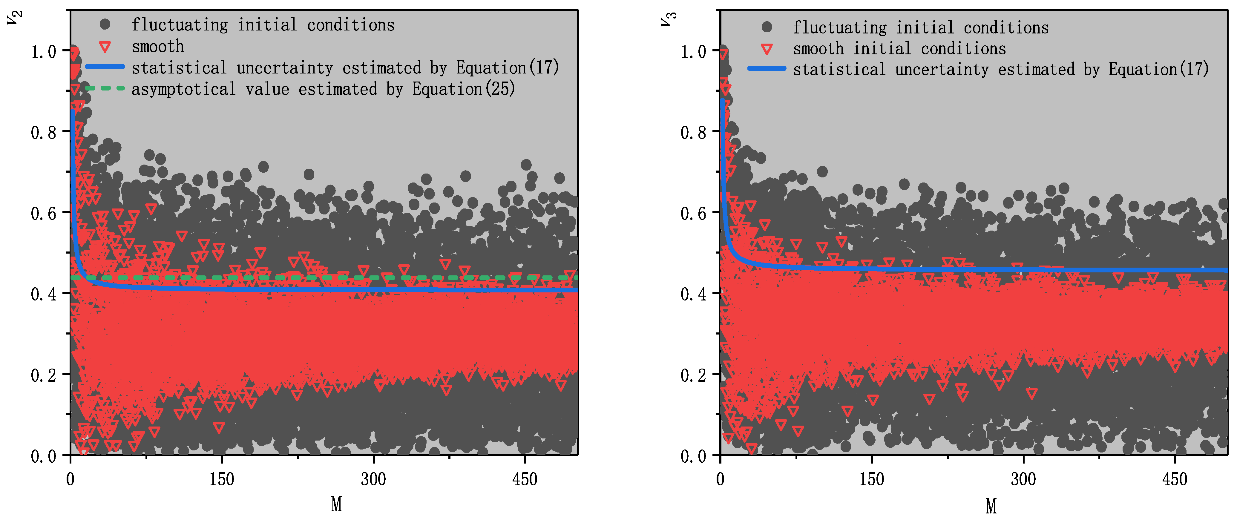
In Figure 1, we present the obtained elliptic and triangular flow coefficients for the generated events of smooth and fluctuating initial conditions. For fluctuating initial conditions, they are prepared according to Equation (3), where one assumes the number of nuggets . Then, the eccentricities are extracted using the definition Equation (2), where the recentering correction is considered. Namely, one replaces z with , where
This leads to for all the events. One can readily verify the numerical implementation by considering the case , which, by the definition Equation (2), one has , free of the event-by-event fluctuations. For simplicity, we adopt the usual assumption that the genuine flow harmonics are proportional to the eccentricities,
For illustrative purposes, it is further assumed that the proportional constant . These flow coefficients, in turn, determine the one-particle distribution given by Equation (1). In the present calculation, the flow harmonics in Equation (1) are truncated at . We employ a Monte Carlo procedure to generate the hardons to simulate the realistic events with a finite multiplicity M. Subsequently, the values of are estimated by the square root of , which is a straightforward generalization of Equation (15). To be specific,
where in our calculations, . As a result, the estimated flow harmonics bear statistical uncertainty due to finite multiplicity in the particle emission according to Equation (1). The results are presented as a scatter plot of estimated flow harmonics as a function of the event multiplicity, vs. M.
For the events with smooth initial conditions, the calculations are rather similar, except that the fluctuations in eccentricities are frozen. One will always take their mean values on the r.h.s. of Equation (21). Again, even though the initial Gaussian distribution is isotropic, the average eccentricities do not vanish.
From Figure 1, it is observed that the flow harmonics are subjected to fluctuations, which decrease with increasing event multiplicity. As expected, the geometrical fluctuations in the initial state give rise to additional uncertainties of flow harmonics on top of those statistical ones. This is demonstrated as the scatters from events of smooth initial conditions mostly sit in a narrower region on top of those generated by fluctuating initial conditions. Moreover, as the event multiplicity increases, such a difference becomes more significant. According to Equation (17), for the events of smooth initial conditions, the variance of flow harmonics decreases with increasing event multiplicity and vanishes at the . On the other hand, for the events generated by fluctuating initial conditions, although the variance of flow harmonics decreases with event multiplicity, they approach a constant value, as further discussed and evaluated below. The above results are confirmed by the quantitative values presented in Table 1, where one estimates the elliptic and triangular flows and their variance. In order to show the robustness of our conclusion, we also carried out calculations using a more significant number . The latter results are presented in Table 2. It is observed that the main feature persists: finite multiplicity gives rise to additional flow variance on top of those due to event-by-event initial conditions.
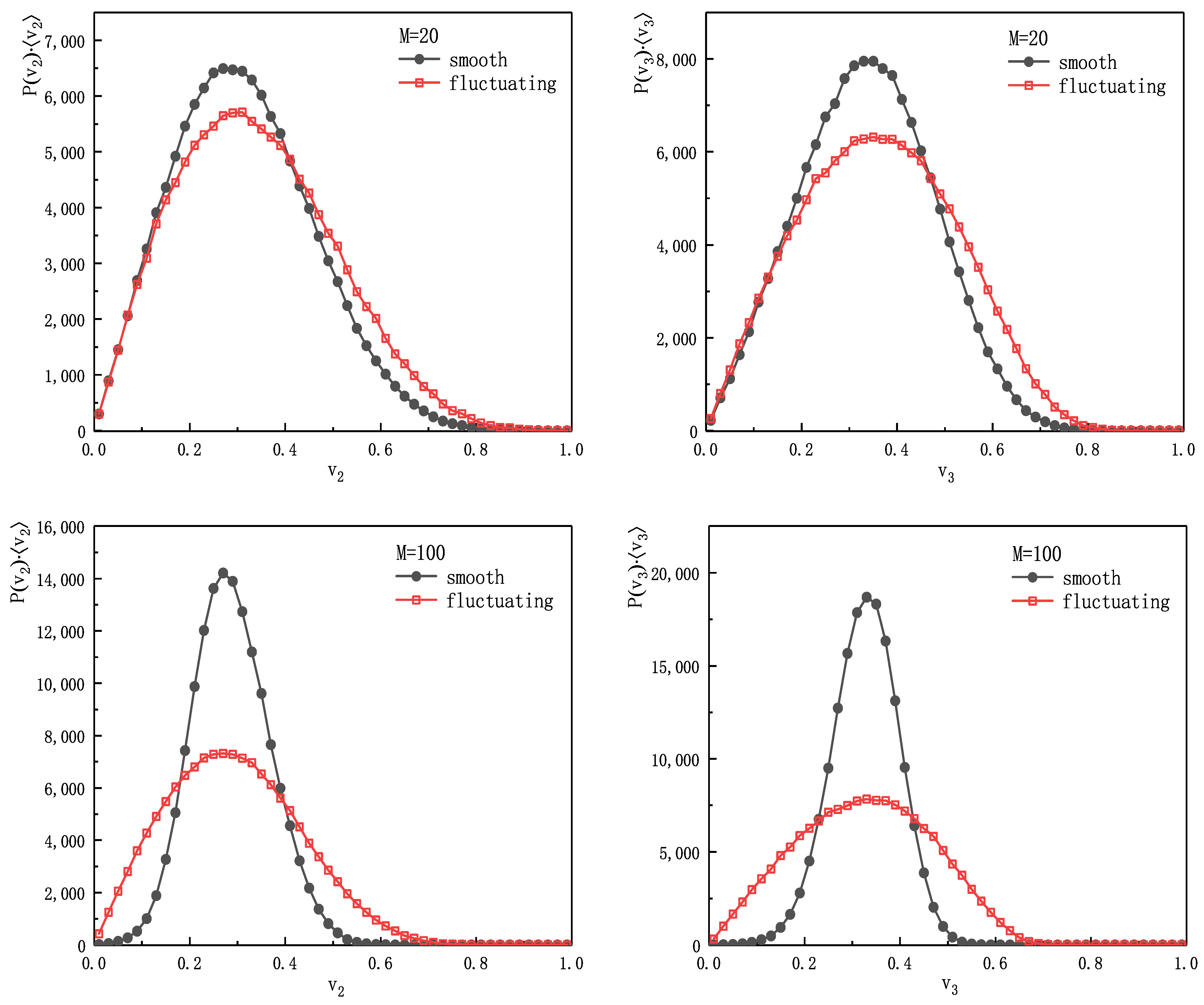
In Figure 2, we present the distribution of the elliptic and triangular flows. Again, the distributions associated with event-by-event fluctuation initial conditions feature a more significant deviation when compared to that associated with the smooth initial conditions. As the number of event multiplicity increases, the variance decreases owing to the suppression of statistical uncertainties, which is consistent with the results shown in Figure 1 and Table 2. Moreover, the difference between the fluctuating initial conditions and smooth ones becomes more significant. Since the probability distribution of flow is a relevant observable, which can be measured experimentally, such a distinction may lead to interesting physical implications.
We now proceed to analyze the above flow fluctuations from an analytic perspective. In particular, we reassess Equations (16) and (17) with the presence of initial eccentricity fluctuations. We will restrain ourselves with the point-source model discussed in Section 2 for the present study. In this case, Equation (16) is replaced by
where one assumes Equation (21).
Similarly, the variance Equation (17) gives
At the limit of infinite multiplicity, the above result gives
which does not vanish as long as N remains finite. Regarding the numerical simulations, the asymptotical value Equation (25) corresponds to the flow variance entirely due to event-by-event fluctuations. It becomes dominant when the event multiplicity M becomes rather significant so that the statistical uncertainties estimated by Equation (17) vanishes. On the other hand, flow fluctuations are completely governed by the statistical uncertainty for the events generated by smooth initial conditions. Compared with the results presented above in Figure 1 and Figure 2, the deviations of flow harmonics due to initial geometric fluctuations and statistical uncertainties are observed to be in accordance with the analytic results.
5. Concluding Remarks
From a statistical viewpoint, we scrutinize the fluctuations in flow harmonics in this work. In particular, we explore two different types of averages. For the first one, one assumes finite multiplicity per event but considers an infinite number of events. For the second case, the average is taken for a given event, where one considers an infinite number of particles at the hydrodynamic limit. Even if one assumes that the elliptic flow is well-defined in Equation (1) without any fluctuation, in the case of events with finite multiplicity, it inevitably gives rise to a finite variance. In this context, we pointed out that one has to adopt a specific scheme to estimate flow harmonics, which is, by definition, a statistical estimator. Due to finite statistics, it is inevitably subject to a finite variance. From the physical perspective, it is argued that for realistic events, the flow fluctuations, demonstrated in terms of the variance of flow harmonics, carry crucial information on both initial-state geometrical and final-state statistical fluctuations. In practice, the two types of variance will be mixed and possibly indistinguishable from that due to the initial state fluctuations, where the latter is understood to carry essential information on the underlying microscopic physical system. A fraction of the event-by-event flow fluctuations are of pure statistical nature. Theoretically, it will only vanish, for instance, as one generates an infinite number of particles in a hydrodynamic simulation.
In terms of experimental observables, notably collective flow and particle correlations, one of the motivations for the extensive numerical simulations for heavy-ion collisions is to distinguish the underlying microscopic mechanisms for the initial conditions. From a hydrodynamic perspective, these distinctions may demonstrate themselves in terms of fluctuations and long-range correlations, which, in turn, might be encoded in the initial conditions by the eccentricities and their fluctuations. In this regard, it is generally understood that hydrodynamics transform the eccentricities mostly linearly into final state flow fluctuations. As discussed above, we argued that the fluctuations in the final flow consist of two components. As a result, if one attempts to extract information on the fluctuations in the initial conditions via flow harmonics and their fluctuations due to finite statistics, finite multiplicity might interfere with such an effort. Event-by-event fluctuations have long become an essential subject in the studies of relativistic heavy-ion collisions. The present study was mainly focused on the aspect of statistical fluctuations, particularly their interplay with those originating from the finite quanta of the relevant system. Moreover, as pointed out in the main text, eccentricities might emerge from the geometrical fluctuations in the initial condition where the continuum limit is taken. Much effort has been devoted to the latter scenarios [11,57,58,59]. Systematically assessing or distinguishing the flow fluctuations associated with different causes is a potentially interesting topic, which might lead to further implications. As shown in Figure 2, the difference in flow variance between the smooth and event-by-event fluctuating initial conditions becomes more significant as the event multiplicity increases, as a result of suppression in statistical uncertainty due to large multiplicity. This result might be physically interesting due to its observable implications. Moreover, given experimental data, the possibility of extracting flow harmonics using a statistical estimator with less variance is also a worthy topic to explore further.
Author Contributions
Conceptualization, methodology, investigation and writing: all the authors; software: C.Y.; validation: C.Y. and W.-L.Q.; All authors have read and agreed to the published version of the manuscript.
Funding
This research is partly funded by the National Natural Science Foundation of China (No. 12047506) the Central Government Guidance Funds for Local Scientific and Technological Development, China (No. Guike ZY22096024). It is also supported by Brazilian agencies Fundação de Amparo à Pesquisa do Estado de São Paulo, Conselho Nacional de Desenvolvimento Científico e Tecnológico, and Coordenação de Aperfeiçoamento de Pessoal de Nível Superior.
Data Availability Statement
The datasets generated and analyzed during the current study are available from the corresponding author upon reasonable request.
Acknowledgments
W.-L.Q. is indebted to insightful discussions with Matthew Luzum and Jean-Yves Ollitrault.
Conflicts of Interest
The authors declare no conflict of interest.
References
- Romatschke, P. New Developments in Relativistic Viscous Hydrodynamics. Int. J. Mod. Phys. 2010, E19, 1. [Google Scholar] [CrossRef]
- Gale, C.; Jeon, S.; Schenke, B. Hydrodynamic Modeling of Heavy-Ion Collisions. Int. J. Mod. Phys. A 2013, 28, 1340011. [Google Scholar] [CrossRef] [Green Version]
- Heinz, U.W.; Snellings, R. Collective flow and viscosity in relativistic heavy-ion collisions. Annu. Rev. Nucl. Part. Sci. 2013, 63, 123. [Google Scholar] [CrossRef] [Green Version]
- Hama, Y.; Kodama, T.; Socolowski, O., Jr. Topics on hydrodynamic model of nucleus-nucleus collisions. Braz. J. Phys. 2015, 35, 24. [Google Scholar] [CrossRef] [Green Version]
- Hama, Y.; Kodama, T.; Qian, W.-L. Two-particle correlations at high-energy nuclear collisions, peripheral-tube model revisited. J. Phys. G 2021, 48, 015104. [Google Scholar] [CrossRef]
- Hirano, T.; Huovinen, P.; Murase, K.; Nara, Y. Integrated Dynamical Approach to Relativistic Heavy Ion Collisions. Prog. Part. Nucl. Phys. 2013, 70, 108. [Google Scholar] [CrossRef] [Green Version]
- Kodama, T.; Stocker, H.; Xu, N. 40 years of collective flow in relativistic heavy ion collisions—The barometer for primordial hot and dense QCD matter. J. Phys. G 2014, 41, 120301. [Google Scholar] [CrossRef]
- de Souza, R.D.; Koide, T.; Kodama, T. Hydrodynamic Approaches in Relativistic Heavy Ion Reactions. Prog. Part. Nucl. Phys. 2016, 86, 35. [Google Scholar] [CrossRef] [Green Version]
- Florkowski, W.; Heller, M.P.; Spalinski, M. New theories of relativistic hydrodynamics in the LHC era. Rept. Prog. Phys. 2018, 81, 046001. [Google Scholar] [CrossRef] [PubMed] [Green Version]
- Danielewicz, P.; Odyniec, G. Transverse Momentum Analysis of Collective Motion in Relativistic Nuclear Collisions. Phys. Lett. B 1985, 157, 146. [Google Scholar] [CrossRef]
- Ollitrault, J.-Y. Anisotropy as a signature of transverse collective flow. Phys. Rev. D 1992, 46, 229. [Google Scholar] [CrossRef] [PubMed]
- Alver, B.; Roland, G. Collision geometry fluctuations and triangular flow in heavy-ion collisions. Phys. Rev. C 2010, 81, 054905. [Google Scholar] [CrossRef]
- Teaney, D.; Yan, L. Triangularity and Dipole Asymmetry in Heavy Ion Collisions. Phys. Rev. C 2011, 83, 064904. [Google Scholar] [CrossRef] [Green Version]
- Qian, W.-L.; Andrade, R.P.G.; Socolowski, O., Jr.; Grassi, F.; Kodama, T.; Hama, Y. p(T) distribution of hyperons in 200-A-GeV Au-Au in smoothed particle hydrodynamics. Braz. J. Phys. 2007, 37, 767. [Google Scholar] [CrossRef] [Green Version]
- Qian, W.-L.; Andrade, R.; Grassi, F.; Socolowski, O., Jr.; Kodama, T.; Hama, Y. Effect of chemical freeze out on identified particle spectra at 200-A-GeV Au-Au Collisions at RHIC using SPheRIO. Int. J. Mod. Phys. E 2007, 16, 1877. [Google Scholar] [CrossRef] [Green Version]
- Hama, Y.; Andrade, R.P.G.; Grassi, F.; Qian, W.L.; Kodama, T. Fluctuation of the Initial Conditions and Its Consequences on Some Observables. Acta Phys. Polon. B 2009, 40, 931. [Google Scholar]
- Andrade, R.; Grassi, F.; Hama, Y.; Qian, W.-L. A Closer look at the influence of tubular initial conditions on two-particle correlations. J. Phys. G 2010, 37, 094043. [Google Scholar] [CrossRef]
- Andrade, R.P.G.; Grassi, F.; Hama, Y.; Qian, W.-L. Temporal evolution of tubular initial conditions and their influence on two-particle correlations in relativistic nuclear collisions. Phys. Lett. B 2012, 712, 226. [Google Scholar] [CrossRef] [Green Version]
- Andrade, R.; Grassi, F.; Hama, Y.; Qian, W.-L. Hydrodynamics: Fluctuating Initial Conditions and Two-particle Correlations. Nucl. Phys. A 2011, 854, 81. [Google Scholar] [CrossRef] [Green Version]
- Castilho, W.M.; Qian, W.-L.; Gardim, F.G.; Hama, Y.; Kodama, T. Hydrodynamic approach to the centrality dependence of di-hadron correlations. Phys. Rev. C 2017, 95, 064908. [Google Scholar] [CrossRef] [Green Version]
- Castilho, W.M.; Qian, W.-L.; Hama, Y.; Kodama, T. Event-plane dependent di-hadron correlations with harmonic vn subtraction in a hydrodynamic model. Phys. Lett. B 2018, 777, 369. [Google Scholar] [CrossRef]
- Wen, D.; Lin, K.; Qian, W.L.; Wang, B.; Hama, Y.; Kodama, T. On nonlinearity in hydrodynamic response to the initial geometry in relativistic heavy-ion collisions. Eur. Phys. J. A 2020, 56, 222. [Google Scholar] [CrossRef]
- Voloshin, S.; Zhang, Y. Flow study in relativistic nuclear collisions by Fourier expansion of Azimuthal particle distributions. Z. Phys. C 1996, 70, 665. [Google Scholar] [CrossRef] [Green Version]
- Niemi, H.; Denicol, G.; Holopainen, H.; Huovinen, P. Event-by-event distributions of azimuthal asymmetries in ultrarelativistic heavy-ion collisions. Phys. Rev. C 2012, 87, 054901. [Google Scholar] [CrossRef] [Green Version]
- Yan, L.; Ollitrault, J.-Y. Universal fluctuation-driven eccentricities in proton-proton, proton-nucleus and nucleus-nucleus collisions. Phys. Rev. Lett. 2014, 112, 082301. [Google Scholar] [CrossRef] [Green Version]
- Qian, W.-L.; Andrade, R.; Gardim, F.; Grassi, F.; Hama, Y. On the origin of trigger-angle dependence of di-hadron correlations. Phys. Rev. C 2013, 87, 014904. [Google Scholar] [CrossRef]
- Qian, W.-L.; Mota, P.; Andrade, R.; Gardim, F.; Grassi, F.; Hama, Y.; Kodama, T. Decomposition of fluctuating initial conditions and flow harmonics. J. Phys. G 2014, 41, 015103. [Google Scholar] [CrossRef]
- Yan, L.; Ollitrault, J.-Y. ν4,ν5,ν6,ν7: Nonlinear hydrodynamic response versus LHC data. Phys. Lett. B 2015, 744, 82. [Google Scholar] [CrossRef]
- Yan, L.; Pal, S.; Ollitrault, J.-Y. Nonlinear hydrodynamic response confronts LHC data. Nucl. Phys. A 2016, 956, 340. [Google Scholar] [CrossRef] [Green Version]
- Bhalerao, R.S.; Ollitrault, J.-Y.; Pal, S. Characterizing flow fluctuations with moments. Phys. Lett. B 2015, 742, 94. [Google Scholar] [CrossRef]
- Grönqvist, H.; Blaizot, J.-P.; Ollitrault, J.-Y. Non-Gaussian eccentricity fluctuations. Phys. Rev. C 2016, 94, 034905. [Google Scholar] [CrossRef] [Green Version]
- Poskanzer, A.M.; Voloshin, S.A. Methods for analyzing anisotropic flow in relativistic nuclear collisions. Phys. Rev. C 1998, 58, 1671. [Google Scholar] [CrossRef] [Green Version]
- Voloshin, S.A.; Poskanzer, A.M.; Snellings, R. Collective phenomena in non-central nuclear collisions. arXiv 2008, arXiv:0809.2949. [Google Scholar]
- Borghini, N.; Dinh, P.M.; Ollitrault, J.-Y. A New method for measuring azimuthal distributions in nucleus-nucleus collisions. Phys. Rev. C 2001, 63, 054906. [Google Scholar] [CrossRef] [Green Version]
- Borghini, N.; Dinh, P.M.; Ollitrault, J.-Y. Flow analysis from multiparticle azimuthal correlations. Phys. Rev. C 2001, 64, 054901. [Google Scholar] [CrossRef] [Green Version]
- Bilandzic, A.; Snellings, R.; Voloshin, S. Flow analysis with cumulants: Direct calculations. Phys. Rev. C 2011, 83, 044913. [Google Scholar] [CrossRef] [Green Version]
- Bhalerao, R.S.; Luzum, M.; Ollitrault, J.-Y. Determining initial-state fluctuations from flow measurements in heavy-ion collisions. Phys. Rev. C 2011, 84, 034910. [Google Scholar] [CrossRef] [Green Version]
- Bhalerao, R.S.; Borghini, N.; Ollitrault, J.Y. Analysis of anisotropic flow with Lee-Yang zeroes. Nucl. Phys. A 2003, 727, 373. [Google Scholar] [CrossRef] [Green Version]
- Bastid, N.; Andronic, A.; Barret, V.; Basrak, Z.; Benabderrahmane, M.L.; Čaplar, R.; Cordier, E.; Crochet, P.; Dupieux, P.; Dželalija, M.; et al. First analysis of anisotropic flow with Lee-Yang zeroes. Phys. Rev. C 2005, 72, 011901. [Google Scholar] [CrossRef] [Green Version]
- Bilandzic, A.; van Kolk, N.; Ollitrault, J.-Y.; Snellings, R. Event-plane flow analysis without non-flow effects. Phys. Rev. C 2011, 83, 014909. [Google Scholar] [CrossRef] [Green Version]
- Bilandzic, A.; Christensen, C.H.; Gulbrandsen, K.; Hansen, A.; Zhou, Y. Generic framework for anisotropic flow analyses with multiparticle azimuthal correlations. Phys. Rev. C 2014, 89, 064904. [Google Scholar] [CrossRef]
- Bhalerao, R.S.; Ollitrault, J.-Y.; Pal, S. Event-plane correlators. Phys. Rev. C 2013, 88, 024909. [Google Scholar] [CrossRef] [Green Version]
- Di Francesco, P.; Guilbaud, M.; Luzum, M.; Ollitrault, J.-Y. Systematic procedure for analyzing cumulants at any order. Phys. Rev. C 2017, 95, 044911. [Google Scholar] [CrossRef] [Green Version]
- Miller, M.L.; Reygers, K.; Sanders, S.J.; Steinberg, P. Glauber modeling in high energy nuclear collisions. Ann. Rev. Nucl. Part. Sci. 2007, 57, 205. [Google Scholar] [CrossRef] [Green Version]
- Kharzeev, D.; Nardi, M. Hadron production in nuclear collisions at RHIC and high density QCD. Phys. Lett. B 2001, 507, 121. [Google Scholar] [CrossRef] [Green Version]
- Kharzeev, D.; Levin, E. Manifestations of high density QCD in the first RHIC data. Phys. Lett. B 2001, 523, 79. [Google Scholar] [CrossRef] [Green Version]
- Drescher, H.J.; Nara, Y. Effects of fluctuations on the initial eccentricity from the Color Glass Condensate in heavy ion collisions. Phys. Rev. C 2007, 75, 034905. [Google Scholar] [CrossRef] [Green Version]
- Drescher, H.-J.; Nara, Y. Eccentricity fluctuations from the color glass condensate at RHIC and LHC. Phys. Rev. C 2007, 76, 041903. [Google Scholar] [CrossRef] [Green Version]
- Drescher, H.; Ostapchenko, S.; Pierog, T.; Werner, K. Initial condition for QGP evolution from NEXUS. Phys. Rev. C 2002, 65, 054902. [Google Scholar] [CrossRef] [Green Version]
- Drescher, H.; Hladik, M.; Ostapchenko, S.; Pierog, T.; Werner, K. Parton based Gribov-Regge theory. Phys. Rep. 2001, 350, 93. [Google Scholar] [CrossRef] [Green Version]
- Werner, K.; Liu, F.-M.; Pierog, T. Parton ladder splitting and the rapidity dependence of transverse momentum spectra in deuteron-gold collisions at RHIC. Phys. Rev. C 2006, 74, 044902. [Google Scholar] [CrossRef] [Green Version]
- Werner, K.; Karpenko, I.; Pierog, T. The ’Ridge’ in Proton-Proton Scattering at 7 TeV. Phys. Rev. Lett. 2011, 106, 122004. [Google Scholar] [CrossRef]
- Werner, K.; Bleicher, M.; Guiot, B.; Karpenko, I.; Pierog, T. Evidence for Flow from Hydrodynamic Simulations of p-Pb Collisions at 5.02 TeV from ν2 Mass Splitting. Phys. Rev. Lett. 2014, 112, 232301. [Google Scholar] [CrossRef] [PubMed] [Green Version]
- Schenke, B.; Tribedy, P.; Venugopalan, R. Fluctuating Glasma initial conditions and flow in heavy ion collisions. Phys. Rev. Lett. 2012, 108, 252301. [Google Scholar] [CrossRef] [PubMed] [Green Version]
- Nahrgang, M.; Aichelin, J.; Gossiaux, P.B.; Werner, K. D mesons in non-central heavy-ion collisions: Fluctuating vs. averaged initial conditions. Nucl. Phys. A 2014, 932, 555. [Google Scholar] [CrossRef] [Green Version]
- Danielewicz, P.; Gyulassy, M. JACOBIAN FREE GLOBAL EVENT ANALYSIS. Phys. Lett. B 1983, 129, 283. [Google Scholar] [CrossRef] [Green Version]
- Bhalerao, R.S.; Ollitrault, J.-Y. Eccentricity fluctuations and elliptic flow at RHIC. Phys. Lett. B 2006, 641, 260. [Google Scholar] [CrossRef] [Green Version]
- Alver, B.; Back, B.B.; Baker, M.; Ballintijn, M.; Barton, D.S.; Betts, R.R.; Bindel, R.; Busza, W.; Chetluru, V.; Garcia, E.; et al. Importance of correlations and fluctuations on the initial source eccentricity in high-energy nucleus-nucleus collisions. Phys. Rev. C 2008, 77, 014906. [Google Scholar] [CrossRef]
- Bhalerao, R.S.; Luzum, M.; Ollitrault, J.-Y. Understanding anisotropy generated by fluctuations in heavy-ion collisions. Phys. Rev. C 2011, 84, 054901. [Google Scholar] [CrossRef]
- Rice, J.A. Mathematical Statistics and Data Analysis, 3rd ed.; Duxbury Resource Center: Duxbury, MA, USA, 2006. [Google Scholar]
Figure 1.
The extracted elliptic and triangular flow coefficients for the events of smooth and fluctuating initial conditions, as a function of multiplicity per event M for . The values of are estimated using given by Equation (22). The hollow red triangles represent the results obtained by the smooth initial condition, and the filled black circles are those by the identical point-source model. The solid blue curve estimates the statistical uncertainties using Equation (17). The dashed green curve shows the asymptotical value of the square root of the variance given by Equation (25) due to event-by-event fluctuations.

Figure 2.
The probability distributions of triangular flow extracted for events of smoothed (black filled dotted) and event-by-event fluctuating (red empty squares) initial conditions generated with . The calculations are carried out by considering different event multiplicities (top row) and (bottom row).


Table 1.
The calculated flow harmonics and their fluctuations using the identical point-source model with . The calculations are carried out for smooth and fluctuating initial conditions with event multiplicity , and 500.
Table 1.
The calculated flow harmonics and their fluctuations using the identical point-source model with . The calculations are carried out for smooth and fluctuating initial conditions with event multiplicity , and 500.
| M | IC | E | Var | E | Var |
|---|---|---|---|---|---|
| 10 | smooth | 0.375 | 0.393 | ||
| fluctuating | 0.397 | 0.409 | |||
| 20 | smooth | 0.316 | 0.338 | ||
| fluctuating | 0.341 | 0.359 | |||
| 50 | smooth | 0.283 | 0.321 | ||
| fluctuating | 0.307 | 0.335 | |||
| 100 | smooth | 0.287 | 0.328 | ||
| fluctuating | 0.292 | 0.324 | |||
| 500 | smooth | 0.295 | 0.331 | ||
| fluctuating | 0.282 | 0.319 | |||
| 1000 | smooth | 0.297 | 0.333 | ||
| fluctuating | 0.289 | 0.317 |
Table 2.
The same as Table 1, but the calculations are carried out for .
Table 2.
The same as Table 1, but the calculations are carried out for .
| M | IC | E | Var | E | Var |
|---|---|---|---|---|---|
| 10 | smooth | 0.312 | 0.342 | ||
| fluctuating | 0.348 | 0.347 | |||
| 20 | smooth | 0.249 | 0.275 | ||
| fluctuating | 0.251 | 0.287 | |||
| 50 | smooth | 0.193 | 0.216 | ||
| fluctuating | 0.215 | 0.242 | |||
| 100 | smooth | 0.173 | 0.207 | ||
| fluctuating | 0.186 | 0.221 | |||
| 500 | smooth | 0.167 | 0.217 | ||
| fluctuating | 0.169 | 0.215 | |||
| 1000 | smooth | 0.174 | 0.213 | ||
| fluctuating | 0.170 | 0.209 |
Disclaimer/Publisher’s Note: The statements, opinions and data contained in all publications are solely those of the individual author(s) and contributor(s) and not of MDPI and/or the editor(s). MDPI and/or the editor(s) disclaim responsibility for any injury to people or property resulting from any ideas, methods, instructions or products referred to in the content. |
© 2023 by the authors. Licensee MDPI, Basel, Switzerland. This article is an open access article distributed under the terms and conditions of the Creative Commons Attribution (CC BY) license (https://creativecommons.org/licenses/by/4.0/).
Share and Cite
MDPI and ACS Style
Qian, W.-L.; Lin, K.; Ye, C.; Li, J.; Pan, Y.; Yue, R.-H. On Statistical Fluctuations in Collective Flows. Universe 2023, 9, 67. https://doi.org/10.3390/universe9020067
AMA Style
Qian W-L, Lin K, Ye C, Li J, Pan Y, Yue R-H. On Statistical Fluctuations in Collective Flows. Universe. 2023; 9(2):67. https://doi.org/10.3390/universe9020067
Chicago/Turabian StyleQian, Wei-Liang, Kai Lin, Chong Ye, Jin Li, Yu Pan, and Rui-Hong Yue. 2023. "On Statistical Fluctuations in Collective Flows" Universe 9, no. 2: 67. https://doi.org/10.3390/universe9020067
Note that from the first issue of 2016, this journal uses article numbers instead of page numbers. See further details here.