


Mu2e Run I Sensitivity Projections for the Neutrinoless μ− → e− Conversion Search in Aluminum
Fermi National Accelerator Laboratory, Batavia, IL 60510, USA
†
Membership of the Mu2e Collaboration is provided in the Appendix A.
Universe 2023, 9(1), 54; https://doi.org/10.3390/universe9010054
Submission received: 25 October 2022
/
Revised: 19 December 2022
/
Accepted: 21 December 2022
/
Published: 13 January 2023
(This article belongs to the Special Issue Charged Lepton Flavor Violation)
Abstract
:The Mu2e experiment at Fermilab will search for the neutrinoless conversion in the field of an aluminum nucleus. The Mu2e data-taking plan assumes two running periods, Run I and Run II, separated by an approximately two-year-long shutdown. This paper presents an estimate of the expected Mu2e Run I search sensitivity and includes a detailed discussion of the background sources, uncertainties of their prediction, analysis procedures, and the optimization of the experimental sensitivity. The expected Run I discovery sensitivity is , with a total expected background of events. In the absence of a signal, the expected upper limit is at 90% CL. This represents a three order of magnitude improvement over the current experimental limit of at 90% CL set by the SINDRUM II experiment.
1. Introduction
Experimental observation of quark mixing and neutrino oscillations proves that interactions of the Standard Model (SM) fermions are non-diagonal in flavor. Cross-generational mixing in the quark and neutrino sectors is large, [1] and [2]. In striking contrast, no indication of flavor mixing has been observed in the charged lepton sector. In the SM with massive neutrinos, charged lepton flavor is only approximately conserved. Virtual loops with mixing neutrinos result in charged lepton flavor violating (CLFV) transitions, regardless of whether neutrinos are Dirac or Majorana particles [3,4]. The branching fractions of the corresponding processes are suppressed by factors proportional to to a level below [5], significantly lower than the sensitivity of any current or planned experiment. Experimental observation of any CLFV process would therefore imply the presence of physics beyond the SM. Many extensions of the SM predict much higher rates of CLFV processes [6], falling within the reach of the new generation of CLFV experiments coming online within the next few years [7,8,9,10,11]. The process of coherent neutrinoless muon to electron conversion in a nuclear field, , probes a wide spectrum of new physics models (see Ref. [12] for general calculations). The present experimental limit on the rate of this process
has been set by the SINDRUM II experiment on a gold target [13].
The Mu2e experiment at Fermilab [9] will search for on an aluminum target with an improved sensitivity of about four orders of magnitude below the SINDRUM II limit. The current Mu2e run plan assumes two data-taking periods, Run I and Run II, separated by an approximately two-year-long shutdown. Run I is anticipated to start in 2025 and collect about 10% of the total expected muon flux, improving the search sensitivity by three orders of magnitude. Run II will further enhance the search sensitivity by another order of magnitude.
This article details estimates of the expected backgrounds and the sensitivity projections for Mu2e Run I. The material is organized as follows. Section 2 describes the Mu2e experiment and the run plan. Section 3 presents an overview of the event simulation framework. Section 4, Section 5 and Section 6 contain discussion of the event reconstruction, trigger simulation, and event selection, respectively. Section 7 describes the background processes, details of their simulation, and gives the estimated contributions from each background source. Section 8 presents the sensitivity optimization procedure and discussion of the results.
2. Mu2e Experiment
2.1. Muon Beamline
The Mu2e experiment is based upon a concept proposed in Ref. [14]. A schematic view of the experiment is shown in Figure 1. Formation of the Mu2e muon beam proceeds as follows. A primary proton beam with = 8 GeV is extracted from the Fermilab Delivery Ring using the slow resonant extraction technique [15]. The beam has a pulsed timing structure, with 250 ns-wide proton pulses separated by 1695 ns. During each 1.4 s main injector cycle, the proton pulses are delivered continuously for about 0.4 s, then the beam is off for the remainder of the cycle. On a millisecond time scale, slow resonant extraction results in significant proton pulse intensity variations [16]. The spill duty factor , where is the variance of the pulse intensity distribution and is the mean pulse intensity, is expected to be above 60%.
The beam interacts with the interaction lengths-long tungsten production target positioned in the center of the superconducting production solenoid (PS). The PS graded magnetic field reaches its maximal strength of 4.6 T downstream of the production target. Most of the particles produced in interactions are pions. Particles produced backwards as well as reflected in the PS magnetic mirror travel through the S-shaped superconducting transport solenoid (TS) towards the superconducting detector solenoid (DS). Muons are mainly produced in decays, which occur in both the PS and TS. The TS magnetic field is also graded, from T at the entrance to about 2.1 T in the region where particles exit the TS and enter the DS. Collimators at the entrance, center, and exit of the TS (COL1, COL3, and COL5) define the TS momentum acceptance, greatly reducing the transport efficiency for particles with momenta above . The curved magnetic field of the TS causes the charged particles of opposite signs to drift vertically in opposite directions—see, for example, Ref. [17]. The vertical separation reaches its maximum in the center of the TS. A vertically offset opening of the rotatable COL3 collimator selects the beam sign, passing through either negative or positive particles. The DS magnetic field has two regions—an upstream region with a graded magnetic field and a downstream region with a uniform field of 1 T.
The inner volumes of all three solenoids are kept at near vacuum. Exposed to the intense proton beam, the radiatively cooled production target will operate at temperatures above 1000 C. Maintaining a low tungsten oxidation rate requires the pressure in the PS region to be kept at torr. To optimize the transport efficiency, suppress backgrounds from secondary interactions, and improve the momentum reconstruction accuracy, the pumping system for the DS region is designed to achieve torr. A thin window in the TS center separates the two vacuum regions.
The stopping target is positioned in the graded B-field region of the DS. The average momentum of the muons entering the DS is , and about one-third of them stop in the stopping target made of 37 Al annular foils spaced 2.2 cm apart. Each foil is 105 m thick and has an inner and an outer radii of 2.2 cm and 7.5 cm respectively. The foils are arranged co-axially along the DS axis.
Muons reaching the stopping target and stopping there come from decays of pions with an average momentum . The average number of stopped muons per primary proton, that is the stopped muon rate, determined from the muon beam simulations is . This number highly depends on the pion production cross section for the protons interacting on the tungsten target. Published measurements of the low-momentum pion production [18,19] are not consistent with each other, so the simulation-based estimate of has a large uncertainty. The impact of this uncertainty on the expected sensitivity is discussed in Section 8.4.
In addition to charged pions, interactions of the proton beam with the production target also produce a large number of ’s. Photons from decays converting in the target result in a flash of low momentum electrons and positrons traveling through the TS and reaching the detector within 150–200 ns from production, as seen in Figure 2. Upon arrival to the DS, the beam flash overwhelms the detector, producing spikes in the detector occupancy. Another consequence of the beam flash is long-term radiation damage to the detectors. Both effects are primarily due to electron bremsstrahlung in the stopping target foils. A significant fraction of the beam flash particles pass through the holes in the foils, reducing the radiation dose absorbed by the detectors by about 30%.
2.2. Signal and Main Backgrounds
Muons stopped in the target foils rapidly cascade to a 1 s orbit in the Al atoms and could undergo the process of conversion. Because in the process of coherent conversion the outgoing nucleus remains in the ground state, the experimental signature of the process is a monochromatic conversion electron (CE) with energy
where is the muon mass, is the recoil energy of the target nucleus, and is the binding energy of the 1s state of the muonic atom. For the Mu2e stopping target material, Al, MeV [20]. Radiative corrections to the conversion electron spectrum have been calculated and are discussed in Ref. [21]. 105 MeV electrons could also come from a number of background processes.
- Cosmic particles interacting and decaying in the detector volume are a source of electrons whose momentum spectrum covers the region around 100 . Most cosmic particles entering the detector are muons; suppression of the cosmic background requires identifying muons and vetoing them.
- Decays in orbit (DIO) of muons stopped in the stopping target and captured by the Al atoms produce electrons with a momentum spectrum extending up to and rapidly falling towards the spectrum endpoint. Observing a peak from conversion in the presence of the DIO background requires searching for the signal in a 1–2 wide momentum window and a detector with an excellent momentum resolution , full width at half maximum (FWHM), ≲ 1 .
- Antiprotons produced by the proton beam and annihilating either in the stopping target or the TS also generate electrons. The antiproton background is suppressed by several absorption elements installed in the TS. Presence of the absorbers reduces the number of stopped muons by ∼5%.
- Radiative capture of pions (RPC) contaminating the muon beam and stopping in the Al target generates a significant background which rapidly falls in time. Suppressing the RPC background requires the live-time window to be delayed with respect to the proton pulse arrival at the production target by several hundred nanoseconds, as schematically shown in Figure 2. The delayed live-time window technique is not efficient against secondary particles produced by protons arriving at the production target between the proton pulses. Suppressing the contribution of those protons requires the proton beam extinction , where is the relative fraction of the beam protons between the pulses.
- Electrons with momenta entering the DS and scattering in the Al stopping target. Similar to RPC, suppressing this background requires the delayed live-time window and an excellent proton beam extinction.
- Decays in flight of negative muons and pions entering the DS and producing electrons with .
- Radiative muon capture (RMC), a process analogous to RPC, but with a lower maximal energy. In aluminum this energy is ∼102 MeV.
The physics processes listed above have very different timing dependencies. The rates of RPC, beam electrons, and decays in flight are strongly correlated with the time of the proton pulse arrival at the production target. The time dependence of the conversion signal, DIO, and RMC are all determined by the lifetime of a muonic Al atom, ns [22]. Cosmic background events are distributed uniformly in time.
2.3. Detector
Momenta of the secondary charged particles produced by decays of nuclear interactions of muons stopped in the stopping target are measured by the straw tracker, located about 3 m downstream of the stopping target in the uniform 1 T region of the DS magnetic field. The tracker is approximately 3 m long and consists of 18 tracking stations, covering radii between 38 cm and 68 cm. It is constructed out of 5 mm diameter straw tubes of different lengths, 20,736 straws in total, filled with a 80%:20% Ar:CO mixture at a pressure of 1 atm. Each straw is read out from both ends, providing two timing measurements for each hit. The difference between the two measured times is used to reconstruct the hit coordinate along the straw. For 100 electrons, the intrinsic momentum resolution of the tracker is expected to be FWHM. For muons of the same momentum, the resolution is slightly worse due to higher energy losses.
Protons from muon captures in the stopping target generate a significant charge load on the tracker. The charge load is reduced by a cylindrical-shaped polyethylene proton absorber placed approximately half-way between the stopping target and the tracker. The proton absorber is 0.5 mm thick, with a radius of 30 cm and a length of 100 cm. Fluctuations of energy losses in the stopping target and the proton absorber dominate the expected momentum resolution in the production vertex FWHM at 100 .
The electromagnetic calorimeter, constructed out of two annular disks covering radii from 37 cm to 66 cm and separated by 70 cm, is positioned immediately downstream of the tracker. Each disk is assembled from 674 undoped CsI crystals, 3.3 × 3.4 × 20 cm in size and read out by two silicon photomultipliers (SiPMs). Tests of the calorimeter prototype using an electron beam have demonstrated, at 100 MeV, energy resolution FWHM, dominated by energy leakage, and timing resolution ps [23]. The inner radius of the instrumented detector region is limited by the rapidly increasing occupancy due to DIO and the radiation damage induced by the beam flash.
Combined together, measurements in the tracker and in the calorimeter provide efficient particle identification and are expected to reduce the background from muons misidentified as electrons down to a negligible level.
For the experiment to reach its design sensitivity, the Cosmic Ray Veto system (CRV), shown in Figure 3, must suppress the cosmic ray background by four orders of magnitude. The CRV consists of four layers of extruded plastic scintillation counters outfitted with wavelength-shifting fibers [24] and read out by SiPMs.
The proton beam extinction is monitored using a magnetic spectrometer with silicon pixel detectors positioned downstream and off-axis of the primary proton beam. The extinction monitor is described in more detail in Ref. [9]. The stopped muon flux is measured by the stopping target monitor consisting of two detectors, a high purity Ge detector and a LaBr detector, located about 30 m downstream of the stopping target and detecting photons emitted in the process of capture in Al.
The data read out from the Mu2e subdetectors are digitized and zero-suppressed by the front-end electronics and transmitted from the detector via optical fibers to the data acquisition system (DAQ). The Mu2e event builder combines the data read out between the two consecutive proton pulses into one event and sends assembled events to a one-level software trigger. To reduce the DAQ rates, the detector readout starts about 500 ns after the proton pulse arrival at the production target when the flux of beam flash particles have already subsided.
A detailed description of the apparatus can be found in the Mu2e Technical Design Report (TDR) [9].
2.4. Mu2e Run I Data-Taking Plan
The Mu2e data-taking plan assumes two running periods, Run I and Run II, separated by an approximately two-year-long shutdown. According to the Run I plan, the experiment will start taking data using a low intensity proton beam with a mean intensity of protons/pulse. Starting at a lower beam intensity facilitates the commissioning of the experiment. During the second part of Run I, the delivered beam will have a higher intensity, with a mean of protons/pulse. About 75% of the total number of protons on target will be delivered in the low intensity running mode, and about 25% in the high intensity running mode. Table 1 summarizes the expected Run I conditions for the two running modes.
3. Simulation Framework
The Mu2e simulation framework is based on Geant4 [25,26,27]. The framework takes into consideration cross sections and time dependencies of the physics processes, timing response of the subdetectors, and effects of hit readout and digitization. All simulations and reconstruction assume perfectly aligned and calibrated detector with no dead channels.
Pileup Simulation
Electron events with are extremely rare. In addition to hits produced by signal-like particle, an event accepted by the Mu2e trigger is expected to have multiple background hits produced by lower momentum particles. Moreover, the Mu2e readout event window is about 1200 ns long, and a realistic detector simulation has to handle particles producing hits in the detector at different times. For the low intensity running mode with the mean intensity of protons/pulse, about 25,000 muons per proton pulse stop in the Al stopping target. About 39% of muons decay in orbit, and about 61% are captured by the Al nuclei, so an average “zero bias” Mu2e event includes ∼10,000 muon DIO and ∼15,000 nuclear muon captures. For the high intensity mode, the corresponding numbers are about 2.5 times higher. The impact of the proton pulse intensity variations is taken into account by approximating them with the log-normal distribution with SDF = 60%. The simulated proton pulse intensity distributions for the low and high intensity running modes are shown in Figure 4. The highest simulated pulse intensity is protons per pulse. The upper cutoff is taken into account in the evaluation of the systematic uncertainties.
The DIO simulation relies on the DIO electron spectrum on Al calculated in the leading logarithmic accuracy in Ref. [28]. Production of different particle species in ordinary nuclear muon captures is simulated using custom event generators tuned to the data to reproduce the inclusive yields. Simulation of protons and deuterons produced in nuclear muon captures relies on their inclusive yields in Al reported in Refs. [29,30]. As there are no published neutron spectra on Al, the simulation of neutrons relies on the neutron spectrum on Ca [31] and assumes 1.2 neutrons emitted per muon capture, in agreement with Ref. [32]. Low energy photons produced in ordinary muon capture are assumed to have a uniform energy distribution from 0 to 7 MeV, with two photons per capture produced on average. The pileup simulation also includes simulation of the beam flash.
4. Event Reconstruction
In contrast to most collider and fixed target experiments, where particles coming from the primary vertex are produced at a known time, the Mu2e event reconstruction has to deal with particles with unknown production times. Timing of all reconstructed primitives—tracks, calorimeter clusters, CRV stubs introduced later in this section—is therefore a parameter determined by the reconstruction, which could vary within hundreds of nanoseconds with respect to the proton pulse arrival at the production target.
4.1. Calorimeter Reconstruction
The Mu2e calorimeter reconstruction processes the digitized waveforms from the calorimeter SiPMs and reconstructs times and energy deposits of the corresponding hits. A single hit waveform is ns long, so resolving hits with overlapping waveforms is an important part of the data processing. Hits with MeV are used to seed a two-pass clustering procedure. For 105 MeV simulated electrons produced at the stopping target, of electrons with a reconstructed track also have a reconstructed calorimeter cluster with MeV. The remaining of electrons go through the central hole or close to the edge of both calorimeter disks and do not deposit enough energy in the calorimeter for a cluster to be reconstructed. The calorimeter reconstruction runs before the track reconstruction. That allows the found clusters to be used to seed the pattern recognition.
4.2. Track Reconstruction
In the momentum region of primary interest, , different charged particle species producing hits in the Mu2e tracker—electrons, muons, and protons—behave very differently. Electrons are ultra-relativistic and have their velocity very close to the speed of the light, . Muons are significantly slower, , and the difference between the electron and muon propagation times through the tracker is large on a scale of a single straw timing resolution. For both electrons and muons, however, the average energy losses in the tracker are on the order of 1–2 MeV, significantly smaller than the particle energy. This is not true for 100 protons which are highly non-relativistic and in most cases lose all their energy in the tracker because of the ionization energy losses. These differences require introducing particle mass-specific corrections at a very early reconstruction stage.
Particles produced at the stopping target pass through the tracker with , and their reconstructed tracks are referred to as downstream tracks. Cosmic ray-induced events often have particles traversing the tracker with . Efficient rejection of the cosmic background therefore requires reconstructing tracks of such particles and tagging them as upstream tracks.
To handle all these different cases, the offline track reconstruction performs several passes. Each reconstruction pass assumes a specific hypothesis about the particle mass and the propagation direction and proceeds in three steps: pattern recognition, fast Kalman fit, and full Kalman fit. Two pattern recognition algorithms, a standalone pattern recognition and a calorimeter-seeded one, are run in parallel. The standalone pattern recognition associates hits with helical trajectories and searches for the track candidates relying only on the straw hit information. The calorimeter-seeded pattern recognition uses reconstructed energetic calorimeter clusters to initiate the track candidate search. It also exploits an assumption that a track corresponds to a particle coming from the stopping target and, by doing that, improves the track finding efficiency for the conversion signal.
The fast Kalman fit does not take into account effects of multiple scattering, energy losses, and the drift times reconstructed in individual straws. It converges within ∼1 ms/event providing a momentum resolution of FWHM. If an event has a reconstructed calorimeter cluster with a position and time consistent with the track, the cluster is included into the Kalman fit, which determines the Z-coordinate of the cluster and its timing and coordinate residuals. A general overview of the first two track reconstruction steps is given in Ref. [33]. The final track reconstruction step, a full Kalman fit, provides the electron track momentum resolution of FWHM at . About 33% of the simulated conversion electron events have reconstructed tracks.
4.3. CRV Reconstruction
Similar to the calorimeter crystals, the CRV counters are read out by SiPMs, and the times and energies of hits in the CRV counters are reconstructed from the digitized waveforms of the SiPM signals. For counters read out from both ends, the time difference of signals read out from the two ends is used to determine the hit coordinate along the counter. The signature of a cosmic muon entering the Mu2e detector is a CRV stub—hits in at least 3 out of 4 CRV layers with a pattern consistent with the pattern of hits produced by a single relativistic particle.
5. Trigger Simulation
The Mu2e trigger system is a one-level online software trigger system. Multiple triggers are implemented as multiple independent reconstruction paths, each path running one or several reconstruction algorithms followed by a software filter to make the trigger decision. The trigger uses the offline reconstruction algorithms with settings optimizing the timing performance. The online track reconstruction path includes two algorithmic steps—a pattern recognition followed by the fast Kalman track fit. The fast Kalman fit provides sufficient, for the trigger, momentum resolution, making it unnecessary to use the full Kalman fit, which is significantly slower. That improves the trigger timing and reduces dependence of the trigger performance on the tracker calibrations.
To improve the trigger efficiency, the two track reconstruction paths exploiting two pattern recognition algorithms introduced in Section 4, are run in parallel. The conversion electron trigger selects events with at least one reconstructed downstream electron track with . The trigger accepts tracks in a wide enough momentum range to enable an analysis of both low-momentum and high-momentum sidebands of the conversion signal.
Figure 5 shows the trigger efficiency for the simulated conversion electron events which have a reconstructed track passing the offline selections. Plotted as a function of the proton pulse intensity, the trigger efficiency varies from 99% at zero beam intensity to 97% at protons/pulse, the highest simulated pulse intensity. Also shown in Figure 5 are the trigger efficiency curves corresponding to the use of the individual pattern recognition algorithms. For the calorimeter-seeded track finding, the trigger efficiency is limited by the calorimeter acceptance and the trigger requirement on the seed cluster energy, MeV. However, the efficiency is almost independent of the beam intensity. In comparison, the efficiency of the trigger based on the standalone tracker pattern recognition at protons/pulse drops by . Stable performance of the trigger based on the OR of the two pattern recognition algorithms illustrates the importance of using both for the online track finding. The expected instantaneous trigger rate is about 60 Hz for the low beam intensity mode.
6. Event Selection
The selection of conversion electron event candidates proceeds in several steps. First, selected event candidates are required to have a track passing the following pre-selection cuts:
- N(hits) ≥ 20: the track has a sufficient number of hits in the tracker.
- < 100 mm: the reconstructed track impact parameter, , is consistent with the particle coming from the stopping target.
- R(max) < 680 mm: the maximal distance from the reconstructed trajectory to the DS axis is less than the radius of the tracker, so the reconstructed trajectory is fully contained within the tracker fiducial volume.
- : the angle between the track momentum vector and the DS axis, at the tracker entrance, is consistent with a track of a particle produced at the stopping target. As the DS magnetic field is graded and is higher at the DS entrance, typical values of for particles entering the DS from the TS are greater than 1.0.
- ns: the uncertainty on the reconstructed track time, , returned by the fit is consistent with a downstream electron hypothesis. This requirement implies that the Kalman fit with the calorimeter cluster included has successfully converged (see Section 4).
Accurate reconstruction of the track momentum is critical for separating the conversion electron signal from the DIO background which rapidly falls with momentum. Especially important is to reject tracks with large positive values of , where is the reconstructed track momentum and is the momentum of the Monte Carlo (MC) particle corresponding to the track, both taken at the tracker entrance. The track selection procedure utilizes an artificial neural network (ANN) trained to separate electron tracks with from tracks with . The ANN training uses tracks passing the pre-selections described above. A detailed discussion of the approach can be found in Ref. [35]. For conversion electron events with tracks passing the pre-selections described above, the efficiency of the ANN-based track selection is 96%. Improvement in the quality of momentum reconstruction is clearly seen in Figure 6—after the track selection, the high-side tail of the distribution is significantly suppressed. The overall track selection efficiency is 81%, so 26% of the simulated conversion events have well reconstructed tracks.
Particle Identification
Most cosmic ray muons entering the detector do not decay within the detector volume. Events with reconstructed muons are discriminated from the events with reconstructed electrons by a particle identification (PID) ANN. The PID ANN is trained using samples of simulated 105 electron and muon events with the reconstructed tracks passing the track selection cuts described in Section 6. Events with muon decays in flight are excluded from the training. The distributions of the output score of the PID ANN, , for electron and muon samples are presented in Figure 7. The requirement identifies events with reconstructed electrons with an efficiency of 99.3%. The corresponding muon misidentification rate is 0.4%.
7. Backgrounds
Optimization of the search sensitivity used in this paper is based on finding the 2D momentum-time signal window maximizing the discovery potential of the experiment. As will be shown in Section 8, the Mu2e Run I discovery potential is optimized for the momentum and time window and ns. The individual background contributions, discussed below, are integrated over this window.
7.1. Cosmic Rays
Interactions and decays of cosmic ray particles in the DS are expected to produce the dominant background in the conversion search. Detailed simulation studies performed using the CRY event generator [36] to simulate the cosmic rays helped identify three distinct types of cosmic background events: (1) cosmic ray muons passing through the CRV coverage, (2) cosmic ray muons entering through the detector regions not covered by the CRV, and (3) neutrally-charged cosmic ray hadrons.
The first type of cosmic ray background events originates from muons striking the detector, or beamline components, and knocking out electrons with energies close to 105 MeV, see Figure 8 (left). Most of the potential background is due to these muons, so this background contribution is primarily determined by the CRV veto efficiency.
The second type of events consists of cosmic ray muons entering the detector through the uninstrumented regions. For instance, there is a significant penetration in the CRV to permit the muon beamline to enter the DS (see Figure 3). Cosmic ray muons can penetrate these regions without being vetoed and produce signal-like particles.
The third type of background contribution originates from the neutral component of cosmic showers, predominantly neutrons, which do not generate signals in the CRV counters. Figure 8 (right) shows a conversion-like event resulting from a cosmic ray neutron interaction in the detector. Cosmic ray neutrons interacting with the material around the stopping target can produce events without an upstream-going electron component. Current estimates suggest that the background from the neutral component does not impact the Run I sensitivity. Comparison of the differential cosmic neutron flux used by CRY to the measurements of Ref. [37] indicates that CRY may be underestimating the neutron component of cosmic showers by a factor of ∼1.5–2. In Run II, the background from cosmic ray neutrons could be reduced with additional shielding.
Cosmic background events have the following characteristic signatures in the Mu2e detector:
- A typical cosmic background event consists of a reconstructed downstream propagating electron and a CRV stub, see Figure 8 (left). The distribution of the timing residuals between the reconstructed electron and the CRV stub is shown in Figure 9. Cosmic event candidates are identified by the timing window ns.
- A cosmic ray particle can also interact in the calorimeter or decay in the tracker volume producing a particle moving upstream, see Figure 8 (right). Both upstream and downstream moving electrons are reconstructed and the upstream component of the track can be used to reject this type of cosmic background events.
Based on the data taking plan for Run I, specified in Table 1, we have estimated the total cosmic background of (stat) events.
Currently, the largest uncertainty on the cosmic background prediction comes from the uncertainty on the CRV counter aging rate. To simulate performance of the counters in Run I, we use results of early Mu2e measurements which yielded an aging rate of 8.7%/year. The ongoing measurements of the counter aging will significantly reduce the associated uncertainties. Current uncertainties of the aging model are not considered in the evaluation of the systematic uncertainties—see discussion in Section 8.
Out of considered sources of the systematic uncertainties the largest contribution comes from the uncertainty on the cosmic flux normalization. The flux of cosmic particles integrated over the data taking time depends on the latitude, altitude, local magnetic field of Earth, etc. In addition, the solar activity cycle, which has a period of about 11 years, makes the integral time-dependent. Based on the data presented in Ref. [38], the uncertainty in predicting the time-dependent intensity of the cosmic particle flux does not exceed 15%. The simulation using a different cosmic shower generator, CORSIKA [39], leads to a 5% different yield of reconstructed electrons per cosmic muon. Added linearly, the two sources give an overall systematic uncertainty of 20% on the cosmic ray background estimate. With the systematic uncertainties included, the cosmic background in Mu2e Run I is . It is worth noting that about 3/4 of the total is due to cosmic muons entering the DS through the area not covered by the CRV.
Reconstructed cosmic event candidates are excluded from the analysis. As the CRV will operate in a high radiation environment, accidental timing coincidences of the reconstructed tracks with CRV hits produced by neutrons and photons from proton beam interactions could mimic cosmic ray muons and introduce an inefficiency in the signal selection. The inefficiencies are estimated at 4% and 15% for the low and high intensity running modes, respectively.
7.2. Muon Decays in Orbit
Electrons produced in decays of free muons at rest have energies up to , well below . However, negative muons stopped in the stopping target get captured by the Al atoms and form muonic atoms. The energy spectrum of electrons from decays of bound muons extends up to , making DIO one of the major background sources to the conversion search. Near the endpoint, the DIO spectrum falls as , driving requirements on the experimental momentum resolution. The leading order (LO) DIO spectrum on Al calculated in Ref. [20] is shown in Figure 10 (left). The leading logarithm (LL) level corrections to the DIO spectrum have been calculated in Refs. [28,40]. Taking into account the higher order corrections lowers the DIO background estimate and as shown in Figure 10 (right), the integral of the DIO spectrum calculated at the LL level over the region [103.6, 104.9] MeV is reduced by % compared to the LO calculation. In this paper, the LL DIO spectrum is used to model the DIO background.
7.2.1. Calibration of the Tracker Resolution and Momentum Scale
A reliable estimate of the DIO background requires understanding of the tracker momentum scale and resolution. Shown in Figure 11 is the distribution of , the momentum resolution of the experiment, for the simulated conversion electrons. here is the CE momentum at the production vertex.
The most probable value of the energy losses in front of the tracker is ∼ 0.5 MeV, and the fluctuations of the energy losses dominate the experimental resolution. The momentum response is well fitted by the following function:
The core part of the resolution function is largely due to the energy losses, and its parameterization is generalized from an approximation to the Landau distribution [41], in which is fixed at 1/2. Introducing in the parameterization allows for an extra degree of freedom which absorbs effects of widening due to the multiple scattering and results in a better fit. The tail on the low momentum side accounts for tracks with large energy losses, while the high-side tail is due to misreconstruction of tracks. Both tails are well described by power law functions. Parameter , the peak position, is defined by the most probable energy losses, is the inverse of the Landau scale parameter [42]. Parameters and determine the transition points from the Landau “core” to the tails. is the overall normalization factor, while , , and are factors determined by the requirement of the continuity of the function and its first derivative. Parameters and determine how fast the power-law tails fall, thus the relative contribution of the tails. The uncertainty on the DIO background resulting from the high momentum resolution tail is dominated by the uncertainty on N.
Parameters of the momentum resolution will be measured as follows. Calibration of the energy losses, parameter , relies on cosmic ray events entering the tracker in the upstream direction, reflecting in the DS magnetic mirror, and returning back to the tracker. Such events have two reconstructed tracks corresponding to the same particle, and the difference between the momenta of the upstream and downstream tracks is defined by the total amount of material crossed by the particle.
Determination of the momentum scale and the core resolution width uses the positive beam. It is based on the reconstruction of the 69.8 positron peak from decays of stopped positive pions. As described in Section 2, switching the beam polarity requires rotating the TS3 collimator by 180 degrees, however, the polarity of the B-field stays the same. An independent calibration of the momentum scale comes from the reconstruction of the momentum spectrum of positrons from Michel decays of stopped positive muons, which has a sharp edge at 52.8 . Both measurements will be performed at a reduced magnetic field to keep the track curvature the same as the curvature of conversion electron tracks at full field.
The measurement of the positron Michel spectrum has a very low background, so the high-momentum tail of the spectrum is dominated by misreconstructed tracks with large . That allows the determination of the parameter from the fit of the high-momentum part of the spectrum.
7.2.2. Systematic Uncertainties
The main sources of systematic uncertainties on the DIO background are listed in Table 2.
- Uncertainty on the absolute momentum scale/ Currently, this is the dominant systematic uncertainty on the DIO background. We expect the momentum scale of the Mu2e tracker to be calibrated to an accuracy of better than 100 at . However, it is not possible to predict the exact value of the resulting systematic uncertainty, so a conservative estimate of 100 is used. Shifting the optimized momentum window by changes the DIO background estimate asymmetrically by [+59%, −37%]. For the high beam intensity running mode, the relative uncertainty is slightly lower. This is expected: at higher occupancy, the momentum resolution degrades, and although the absolute value of the background increases, the slope of the measured DIO spectrum becomes less steep, reducing the relative uncertainty.
- Uncertainty on the momentum resolution tail. The momentum resolution function shown in Figure 11 has a non-Gaussian tail on the high-momentum side. As the DIO spectrum is rapidly falling towards the endpoint, the uncertainty on the tail may lead to a non-negligible uncertainty on the expected background. The resolution tail at 100 can not be studied directly using the data—there is no physics process which could be used for that. We therefore plan to perform a detailed study of the detector momentum response using the sharp high energy (∼52 MeV) edge of the positron spectrum measured from the decays of stopped positive muons. The magnetic field in the tracker will be reduced by ∼50% to match the curvature of the reconstructed positron tracks with the curvature of the conversion electron tracks in the nominal magnetic field. Below, we outline the proposed method and demonstrate that its intrinsic uncertainty is small.From Equation (2), the uncertainty on the tail is dominated by the uncertainty on the parameter N. A direct fit of the resolution function for simulated 52.8 positrons, shown in Figure 12 (left), returns . To determine the value of from the analysis of the Michel spectrum, we assume that all parameters in Equation (2), except , are fixed from the studies of cosmic and events, and for the present study their values are taken from the fit of the 52.8 positron dataset. A convolution of the theoretical Michel spectrum with the resolution function corresponding to different values of produces multiple templates. Each template is used to fit the spectrum of Michel positrons simulated and reconstructed in B = 0.5 T, with the only floating parameter in the fit being the overall normalization. The analysis of the distribution dependence on yields the best value of . The best fit is shown in Figure 12 (right). The two results are statistically consistent, and their relative difference of 14% can be used to estimate the systematic uncertainty of the method. Assuming the relative uncertainty scales with the track curvature, the resolution function for 100 electrons reconstructed at B = 1 T should have the same relative uncertainty on . Under this assumption, convolving the momentum resolution function at 105 from Figure 11 with the DIO spectrum results in the relative uncertainty on the DIO background of . This uncertainty, contributed to by the experimental procedure, is already small compared to the uncertainty due to the momentum scale and can be further reduced in the future.
7.2.3. Expected Yield of the DIO Electrons
The DIO background normalized to the stopped muon flux of Run I is shown in Figure 13. The estimated DIO background for Mu2e Run I is 0.038 ± 0.002(stat) (syst).
7.3. Radiative Pion Capture
RPC occurs when pions contaminate the muon beam and stop within the stopping target. The stopped pions undergo the process , followed by an asymmetric conversion producing electrons with an energy spectrum extending above 130 MeV. This is one of the main background sources to the search. Emission of virtual photons with is a direct source of pairs. Following Refs. [43,44], this process is referred to as internal conversion. By extension, the conversion of on-shell photons in the detector material is referred to as the process of external conversion. Compton scattering of on-shell RPC photons in the detector also produces background electrons. This causes an increase in the RPC background electron yield for external conversions and makes the spectra of electrons and positrons differ.
The internal conversion fraction (), the ratio of the off-shell and on-shell photon emission rates, has been calculated in Refs. [43,44]. In this analysis, the internal conversion fraction is assumed to be independent of the photon energy, and the value of , measured in Ref. [45], is used.
The RPC background modeling relies on the RPC measurements on nuclei published in Ref. [46]. As there is no published data on Al, the spectrum of RPC photons measured on a Mg target is used. According to Ref. [46], for nuclei with the nuclear charge Z in the range , the measured RPC branching ratio varies by . Although the measured spectra are not exactly the same, the difference between Al and Mg should not introduce a significant additional systematic uncertainty.
7.3.1. RPC Sources
A pulsed timing structure of the proton beam leads to two distinct components of RPC background:
- In-time RPC: radiative capture of pions produced by protons arriving in the beam pulse. The rate of in-time RPC rapidly decreases with time roughly following the negative pion lifetime, and the corresponding background can be minimized by sufficiently delaying the live-time search window with respect to the beam pulse.
- Out-of-time RPC: radiative capture of pions produced by out-of-time protons. A delayed live-time window cannot eliminate such pions, only extinction of out-of-time protons can do this.
A third source of delayed RPC background results from antiproton annihilation in the transport solenoid and is described in Section 7.5.
7.3.2. Momentum and Time Distributions
Figure 14 shows the distributions of the reconstructed track momentum and time for in-time RPC electrons. All track selection criteria are enforced except for momentum and time cuts. The plots are normalized to represent the number of protons on target expected in Run I. The RPC photon spectrum with the endpoint at ∼134 defines the maximal momentum of the reconstructed electrons, and below ∼80 the reconstruction is limited by the tracker acceptance. RPC photons contributing to the background predominantly convert in the same stopping target foil in which they were produced. Due to the small thickness of the stopping target foils, the contribution of external conversions is about 50% lower than the contribution of internal conversions. The time distribution displays a characteristic exponential slope. Pions produced by out-of-time protons can arrive at the stopping target at any point within the event and, consequently, the time distribution for out-of-time electrons is assumed to be flat.
The estimated contribution of the in-time RPC is events. The contribution of the out-of-time RPC, proportional to the proton beam extinction, is events.
7.3.3. Systematic Uncertainties
- RPC Photon SpectrumA RPC branching rate of , taken from Ref. [46], is used in this study. A relative uncertainty of 9.3% on this measured rate is assigned as the corresponding systematic uncertainty on for Al.
- Internal Conversion FractionThe internal conversion fraction measured in Ref. [45], , is used. Its value is assumed to be independent of the photon energy. The measurement presented in Ref. [45] was performed using hydrogen, where MeV. As the energy region of interest for the conversion search is around 105 MeV, and the theory predicts a decrease of as the photon energy goes down, this assumption is conservative.
- Proton Pulse ShapeThe variation in the pion-capture background due to uncertainty in the simulated shape of the incoming proton beam time structure was found to be negligible.
- Pion Production Cross SectionThe Run I data taking plan assumes collection of stopped negative muons (see Table 1). As muons are primarily produced in pion decays, one might think that the ratio of the number of stopped negative pions to the number of stopped negative muons, , is constant, and that, for a fixed number of stopped muons, the RPC background would not depend on the pion production cross section. However, the pions which stop in the stopping target have momenta significantly lower than the pions producing stopped muons, so the ratio depends on the energy spectrum of the produced pions. As there is no experimental data on production of charged pions with momenta below 100 , model-dependent predictions have to be used. For a fixed number of stopped negative muons, different hadro-production models implemented in Geant4 predict variations of the RPC background. The relative change in the RPC background yield depends on the model used, and results in an asymmetric systematic, shown in Table 3.
7.3.4. Summary of Systematic Uncertainties on the RPC Yield
Table 3 lists all the systematic uncertainties discussed. For each column the contributions are added in quadrature to provide total uncertainties. It must be noted that the major systematic uncertainties in this result come from assumptions made within our modeling and can be reduced through using a data-driven estimate.The RPC yield could potentially be estimated through measurements of electrons from pions arriving early at the stopping target (before any conversion electron is expected). They could be fitted with an exponential expression and the yield in the signal region could be extrapolated from that fit. It is important to note that data from Run I can be used to measure the RPC photon spectrum and RPC branching fraction in aluminum, and also help validate our pion production cross section model, thus reducing systematic uncertainties in future physics runs.
With the systematic uncertainties included, the expected background contributions of the in-time and out-of-time RPC are and , respectively.
7.4. Radiative Muon Capture
The process of radiative muon capture, , in many aspects is similar to RPC. The theoretical framework developed to describe internal pair production in nuclear RPC [43] is general enough to include nuclear RMC, and the probability of internal RMC conversion is defined by a very similar calculation [47].
However, there are also important differences. The maximal energy of the RMC photon, defined by the muon mass, is about 34 MeV lower than the maximal energy of the RPC photon, which is defined by the charged pion mass. For Al, the maximal energy of the RMC photon is MeV, about 3 MeV below the expected conversion signal. The timing dependence of the RMC electron rate is defined by the lifetime of the muonic aluminum atom, common for all processes which proceed through muon capture.
The energy spectrum of the RMC photons is also very different from the spectrum of RPC photons. General features of the RMC spectra are well described within the closure approximation, which replaces the sum over transitions into multiple final nuclear states with a transition into a single state with the mean excitation energy [48]. Within the closure approximation, the RMC photon spectrum is fully defined by one parameter—the endpoint of the photon spectrum, :
where and . [48]. The closure approximation captures reasonably well the total RMC rate and the shape of the RMC photon spectra, however, as is a model parameter, it can not be relied upon to determine the spectrum endpoint. Typically, the closure approximation fits return values 5–10 MeV below the kinematic limit. For example, for a RMC transition, the maximal kinematically allowed photon energy is MeV, while fits to the experimental data return MeV [49].
As the conversion electron energy is MeV and the Mu2e momentum resolution FWHM, the background from RMC, estimated using the closure approximation spectrum with the endpoint of , is negligible. As there is nothing that explicitly forbids RMC photons up to the kinematic limit, it is reasonable to assume that the spectrum has a tail up to this limit with an event rate too low to have been measured by the performed experiments. To test the sensitivity of the conversion search to this assumption, the RMC photon spectrum on aluminum described by Equation (3) with = 90.1 MeV is modified by adding to it a tail extending up to the kinematic limit. Two parameterizations of the tail are considered: (1) a closure approximation spectrum with = 101.9 MeV and (2) a flat distribution.
The first choice is similar to that used in Ref. [50], while the second choice ignores the phase space reduction and should result in an overly-conservative background estimate. In each case, the tail is normalized to 3 events above 90 MeV in the previous measurement, which is close to the sensitivity limit of Ref. [49]. The chosen normalization corresponds to a rate of . The two parameterizations of the RMC photon tail are shown in Figure 15 along with the closure approximation fit of Ref. [49], normalized to the number of stopped muons expected in Run I.
Table 4 gives the background estimates for both considered parameterizations of the tail in the optimized signal window introduced in Section 7. The dominant contribution comes from the on-shell photons: for the same photon energy, Compton scattering produces electrons with a momentum spectrum that extends higher than the spectrum of pair-produced electrons. Table 4 shows that even under an overly-conservative assumption the RMC background to the conversion search is negligibly small. However, the high energy tail of the RMC photon spectrum may modify the total electron spectrum around 100 and impact measurements of the high-momentum end of the DIO spectrum.
The value of events is used as a conservative upper limit on the expected RMC background.
7.5. Antiprotons
Another potentially significant source of background is due to the annihilation of antiprotons produced in the interactions of the GeV proton beam at the tungsten target and entering the TS. Such antiprotons can pass through the TS, enter the DS, and annihilate in the stopping target producing signal-like electrons. In addition, radiative capture of negative pions produced in the antiproton annihilation along the beamline and reaching the stopping target increases the overall RPC background, adding a component with a time dependence very different from those discussed in Section 7.3.
The background induced by antiprotons cannot be efficiently suppressed by the time window cut used to reduce the prompt background because the antiprotons are significantly slower than the other beam particles and their secondary products are delayed with respect to the beam. The only way to suppress the antiproton background is to use additional absorber elements, located at the entrance and at the center of the TS. The antiproton background estimate is mostly affected by the uncertainty on the antiproton production cross section that has never been measured at such low energies.
7.5.1. Antiproton Production Cross Section
The Mu2e primary proton beam has a momentum of , but the lowest proton momentum at which cross section experimental data are available is 10 (Table 5).
To generate antiprotons from protons of any momentum the invariant differential cross section () has been parametrized as a function of the antiproton momentum () in the center of mass system (c.m.).
In the simple case of a interaction,
the maximum () corresponds to the case in which the three protons in the final state act as a single body and recoil in the direction opposite to the :
where s is the Mandelstam invariant variable and is the proton mass.
When the nucleus, tungsten in the case of Mu2e, is considered as the target,
more nucleons can be involved in the interaction and the antiproton momentum in the c.m. can be larger than . The ratio is then correlated to the multi-nucleon state participating in the interaction. The concept of the fraction of maximum momentum in the c.m. can be improved using the variable
where the dependence on the antiproton angle in the c.m. system with respect to the incident proton direction () takes into account the different matter density seen by the particle in case of forward or backward scattering and is a parameter that ensures a smooth transition between the forward and the backward region. The value of is obtained by fitting the data.
The parametrization of the invariant cross section as function of is given by Ref. [56]:
where and the parameters obtained by fitting the data are:
Figure 16 shows the fit to the data in the c.m. system and in the laboratory system. The normalization of the exponential term in Equation (8) is fixed by the continuity requirement at . The normalization of the measurements at a given angle, that come from the same publication, has also been used as a fit parameter. The relative change in the normalization for each input dataset is shown in the legend.
The fit to the data at 10 (Figure 16) is quite good, and the corresponding total cross section is 282.4 b. Using an incident proton momentum of 8.9 , that is the Mu2e beam momentum, the total cross section goes down to 213.2 b, that is 75% of the cross section at 10 .
This result can be compared with the one obtained using the simple model proposed in Ref. [57], where the total cross section has been parametrized as a function of the Mandelstam invariant variable s, neglecting the interaction with multinucleon states:
from which one gets:
where and are the total antiproton production cross sections for the proton beam momenta of 8.9 and 10 respectively. As shown in the same paper, the effect of the interaction with more nucleons is expected to become larger and larger when approaching the antiproton production threshold, so that Equation (9) becomes less and less valid.
The discrepancy between the results of the two parametrizations reflects the uncertainty in the cross section extrapolation to lower energies where no experimental data are available. At this point, the only statement that can be made is that the cross section at 8.9 must be lower than the one at 10 . According to this quite conservative assumption, the antiproton production cross section at 8.9 can be taken as:
7.5.2. Antiproton Simulation
The antiproton simulation has been performed in several steps. First, vertices of inelastic proton beam interactions in the production target were simulated and stored. The number of antiprotons produced in the production target () per POT is given by:
where is the total antiproton production cross section obtained integrating the differential cross section in Equation (11), is the probability, obtained by Monte Carlo, that a proton in the beam produces an inelastic interaction in the tungsten target, and mb is taken from Ref. [58]. This value for the total proton inelastic cross section on tungsten is higher than the value of 1517 mb obtained with MCNP [59], but this discrepancy can be neglected with respect to the 100% error quoted for the cross section extrapolation at threshold.
In the second step of the simulation, the proton inelastic vertices were used as production vertices of antiprotons generated with the momentum distribution flat between 0 and 5 and isotropic in direction. The generated antiprotons were propagated to the TS entrance to determine the TS acceptance as a function of the antiproton momentum and emission angle. The calculated TS acceptance has been used to build a significantly more efficient generation model, where the probability to generate an antiproton with a given momentum and a polar angle was proportional to the antiproton production cross section used by Geant4 and the square root of the TS acceptance. To avoid reliance on the Geant4 modeling of the antiproton production, the weights of the generated antiproton events have been corrected by the ratio of the parametrized invariant cross section of Equation (8) and the inclusive cross section used by Geant4.
The TS acceptance calculation by Geant4 was cross-checked against simulations based on FLUKA [60], MARS [61], and MCNP. Compared to Geant4, all three MC codes produced a much higher fraction of back-scattered antiprotons. For this reason, the TS acceptance has been corrected by introducing an additional event weight defined by the ratio of the MCNP and Geant4 acceptances—see Figure 17 (left).
Figure 17 (right) shows the two-dimensional distribution of vs. p for antiprotons reaching the TS, where p and are the momentum and the polar angle of the generated antiproton at its production vertex.
An antiproton reaching the TS can be produced by the interaction of the generated antiproton. This is usually the case for the forward produced antiprotons. The antiprotons emitted in the direction of the TS () can in principle have any momentum but because of the cross section have essentially . The ones generated in the direction opposite to the TS () are much more enhanced by the cross section and a small but relevant fraction of them undergo secondary interactions in the production target producing a secondary antiproton reaching the TS.
To optimize the simulation time, each antiproton reaching the TS entrance is resampled times. It has been verified that, given the large amount of material crossed by the antiprotons from the TS entrance to the stopping target, this resampling factor does not significantly affect the final statistical error. A set of optimized absorbers has been added at the entrance and the center of the TS to suppress antiproton backgrounds while minimizing the introduced delayed RPC backgrounds and not significantly affecting the number of muons stopped in the stopping target. The expected number of antiprotons stopped in the stopping target in Run I is
where the systematic error is dominated by the uncertainty on the production cross section (Equation (11)).
The space and time distribution of the stopped is shown in Figure 18. Most of the antiprotons stop in the first aluminum foil of the stopping target. The stopping time can be within the conversion electron search window.
Antiproton annihilations in the stopping target are simulated using the position and time of the stopped antiprotons. The background electrons produced in these annihilations are due to decays followed by the photon conversions and decays followed by the negative muon decays. The background due to antiproton annihilations in the signal momentum and time window for Run I is .
7.5.3. Delayed RPC Simulations
The background due to the pions produced before the TS is considered as standard RPC background, whether the pions come from a proton interaction or from an antiproton annihilation. An additional antiproton-induced background comes from pions produced by antiproton interactions inside the TS. These pions arrive at the stopping target later, and electrons resulting from their captures are more likely to pass the timing cuts used to select the CE signal. The first stages of the delayed RPC simulation are the same as used for the antiprotons. Starting from the TS, the pions produced by antiproton annihilations are traced down to the stopping target: they can decay along the way or, eventually, reach the stopping target and stop there. Figure 18 shows the time and position of pion stops in the stopping target. A peak in the timing distribution around 300 ns corresponds to pions produced in the first antiproton absorber positioned in front of the TS. A broad distribution with the maximum around 500–600 ns is due to pions produced in antiproton annihilations in the second absorber located in the middle of the TS.
The times and positions of the pion stops are used to produce RPC events. As with the standard RPC background, the background contribution of both the virtual (internal conversions) and the real (external conversions) photons have been estimated separately and added up. Assuming the proton extinction is better than , the contribution of the out-of-time protons is negligibly small, and the background due to the delayed RPCs in the signal momentum and time window for Run I is . The delayed RPC background is a significant component of the antiproton background, constituting 22% of the total. As for the annihilations, the dominant systematic error for the estimate of this background is given by the uncertainty on the antiproton production cross section (Equation (11)).
7.6. Other Background Sources
Several small beam-related background contributions are due to particles not stopping in the stopping target. All of them originate from protons arriving at the production target between the proton pulses and are suppressed by the proton beam extinction.
- Beam electrons with momentum around 105 that arrive at the stopping target and scatter there could get reconstructed in the detector and fake the signal. The main source of such electrons are muons decaying in the downstream half of the TS and in the DS, in front of the stopping target. The small, , probability of a large angle scattering in the stopping target combined with the beam extinction of reduces the expected contribution from beam electrons to a level below events;
- Negative muons and pions that enter the DS and decay in flight there, producing electrons with momenta above 100 . The electrons could get reconstructed without scattering in the stopping target and mimic the conversion signal. The estimated contribution from decays in flight is below events.
- The expected background from the DIO of muons stopped in the TS is negligibly small.
Because of their small expected values, the backgrounds described in this section are not considered in the sensitivity optimization procedure.
8. Sensitivity Optimization
8.1. Optimization Strategy
The experimental sensitivity estimate in this analysis is based on simple event counting. The event counting is performed in a two-dimensional momentum and time signal window, so the optimization of the experiment’s sensitivity to discovery is reduced to the optimization of the signal window limits.
A standard measure of an experiment’s ability to make a discovery is its “median discovery potential” characterized by the minimal signal strength for which, given the mean background expectation , the probability to satisfy the discovery criterion would be at least 50%. Standard for HEP, a discovery is defined as a measurement yielding a significant, “5”, deviation from the expected background and corresponding to a p-value of . While this definition is very clear, it may not provide the best figure of merit for the sensitivity optimization. Due to the discrete nature of the measurement, the same number of events is needed to claim a discovery for a range of values. In this case, higher background values correspond to better sensitivities, which is rather counter-intuitive. A better figure of merit is the average discovery potential, defined as the signal strength that corresponds to an average deviation from the background-only hypothesis. The average deviation is determined by assuming the Gaussian probability distribution, converting the p-value of each generated pseudo-experiment into the number of standard deviations , and calculating an average value of the distribution of . Using the average discovery potential avoids the known pathologies of the median discovery potential—see the discussion by Bhattiprolu et al. comparing these and other methods of quoting the discovery potential [62]. It is also similar to the method proposed by Feldman and Cousins (FC), where the average of the distribution of upper limits from pseudo-experiments, as opposed to the median expectation, is used to quantify the experimental sensitivity [63]. To combine the best of both approaches—avoid numerical pitfalls in the optimization procedure and have a clear definition of the discovery potential—the sensitivity optimization is performed in two steps. First, the sensitivity is optimized using the “mean” definition of the signal strength as the figure of merit, and the position and size of the two-dimensional signal window are determined. Next, the “median” signal strength is calculated for the optimized selection and used to quote the discovery sensitivity and the expected upper limits.
8.2. Optimization of the Momentum and Time Signal Windows
The upper and lower edges of the momentum and time windows are optimized using the mean discovery potential described above. The rapid rise of the DIO momentum distribution prevents the optimization from moving the lower edge of the momentum window significantly below . Similarly, extending the window above 105 does not improve the signal acceptance, adding only the background. The lower edge of the timing window is constrained by the RPC background, the contribution of which becomes large, on a scale of 0.01 events, for below 650 ns. To avoid background from the flash from the next proton pulse, the maximal value of T is set to 1650 ns.
The momentum and time windows are optimized using a grid search in steps of 50 in momentum and 10 ns in time for both the upper and lower edges of the windows. The optimized momentum window is and the optimized time window is ns, as introduced in Section 7. One of the parameters characterizing the sensitivity of an experiment to a process of interest is its single event sensitivity (SES), defined as the signal strength corresponding to a mean expectation of one observed signal event. The optimized Mu2e signal window corresponds to a SES of and a total signal reconstruction and selection efficiency of .
8.3. Including Systematic Uncertainties
The signal window optimization is performed without taking systematic uncertainties into account. After the optimal signal window is determined, the expected sensitivity is recalculated with the systematic uncertainties included. The expected sensitivity is optimized assuming a fixed number of stopped muons, , defined in Table 1. The included uncertainties represent the current best estimate of what they will be at the time the analysis is performed. The systematic uncertainties are treated as nuisance parameters with specified probability density functions (PDF). Uncertainties associated with the current predictions of the detector performance are not used at this step. An example of such uncertainty is an uncertainty of predicting the CRV light yield during the data-taking. The construction of the FC confidence belts in the presence of systematic uncertainties follows the method described in Ref. [64], with numerical approximations made to speed up the execution.
Table 6 lists the systematic uncertainties. Uncertainties on the PID and the track reconstruction efficiency are expected to be significantly smaller than 5%, so Table 6 does not include them.
In the sensitivity calculation, the uncertainties are implemented using log-normal PDFs. In case of asymmetric errors, the larger uncertainty value has been used to parameterize the PDF. The choice of log-normal representation of PDFs avoids negative background expectations. In addition, compared to the choice of Gaussian representation, it results in more conservative sensitivity estimates.
Systematic uncertainties on the DIO and the signal acceptance are dominated by the uncertainty on the momentum scale. Reducing the momentum scale uncertainty below 100 keV/c would help reducing those uncertainties. In-situ measurement of events with cosmic muons will significantly reduce the uncertainty on the cosmic flux normalization. Direct Mu2e measurement of the RPC cross section will eliminate the uncertainty on the RPC background related to the pion production cross section. A 10% uncertainty of the stopped muon flux normalization will be achieved by the combination of measurements with the stopping target monitor and the measurements of the DIO rate and the RMC cross section on Al. A published uncertainty on the latter is slightly better than 10% [49].
8.4. Sensitivity Estimate
Table 7 presents the Mu2e Run I discovery potential and exclusion limit with and without the systematic uncertainties included. The 5 discovery , and claiming a signal requires an observation of 5 or more events. Taking the systematic uncertainties into account degrades the expected sensitivity values by about 10%. As shown in Figure 19, for this value, the observed number of events with a probability of about 75%. The background summary after the sensitivity optimization is given in Table 8.
Estimating the sensitivity for a fixed number of stopped muons makes the estimate largely independent of one of the current largest experimental uncertainties, the uncertainty on the stopped muon rate, . A change in the stopped muon rate changes the data-taking time needed to collect the required number of stopped muons, and through that, the cosmic ray background. A stopped muon rate twice as low as the number used for the sensitivity estimate would increase the running time by a factor of two and double the cosmic ray background. However, the total background would increase by only about 50%, changing the median discovery by less than 5%. Moreover, a total background increase by a factor of three would degrade the discovery by only about 30%.
Alternatively, for a constant data taking time, the discovery would scale approximately as .
The current world’s best limit on the conversion search, at 90% CL, has been set by the SINDRUM II experiment on an Au target [13]. Compared to SINDRUM II, in Run I, Mu2e is expected to improve the search sensitivity by a factor of more than 1000.
Figure 20 shows the momentum and time distributions for the signal and individual background processes corresponding to the optimized signal window.
9. Summary
We present an updated estimate of the expected Mu2e sensitivity to the search for the neutrinoless conversion on an Al target. Mu2e Run I, the first part of the Mu2e data-taking plan described in Section 2.4, assumes an integrated flux of stopped muons. The discovery corresponding to a 50% probability of observing the conversion signal at a significance level is . Reaching the significance level requires observing 5 candidate events in the two-dimensional search window , ns. The corresponding expected background is events, significantly lower than one event.
In the absence of a signal, the expected 90% CL upper limit on the conversion rate is , a factor of improvement over the current experimental limit at 90% CL [13].
In the second part of the data-taking plan, Run II, Mu2e is expected to improve the experimental sensitivity of the conversion search by another order of magnitude.
Funding
This work was supported by the US Department of Energy; the Istituto Nazionale di Fisica Nucleare, Italy; the Science and Technology Facilities Council, UK; the Ministry of Education and Science, Russian Federation; the National Science Foundation, USA; the National Science Foundation, China; the Helmholtz Association, Germany; and the EU Horizon 2020 Research and Innovation Program under the Marie Sklodowska-Curie Grant Agreement Nos. 734303, 822185, 858199, 101003460, and 101006726. This document was prepared by members of the Mu2e Collaboration using the resources of the Fermi National Accelerator Laboratory (Fermilab), a U.S. Department of Energy, Office of Science, HEP User Facility. Fermilab is managed by Fermi Research Alliance, LLC (FRA), acting under Contract No. DE-AC02-07CH11359.
Institutional Review Board Statement
Not applicable.
Informed Consent Statement
Not applicable.
Data Availability Statement
MC datasets generated during this study could be obtained by request from the Mu2e collaboration.
Acknowledgments
We are grateful for the vital contributions of the Fermilab staff and the technical staff of the participating institutions.
Conflicts of Interest
The authors declare no conflict of interest.
Appendix A. Membership of the Mu2e Collaboration
Byrum K. Corrodi S. Oksuzian Yu. Winter P. Xia L. Wagner R. Carey R. M. Edmonds A. Israel S. Miller J.P. Mott J. Barnes E. Palladino A. Jorjadze V. Khalatian V. Quirk J. Roberts B. L. Song H. Tran N. Wang Y. Marciano, W. J. Ding, D. Herman, A. Hirsh, S. Kolomensky, Yu. G. Singh, V. Varier, D. Harrig, K. Nguyen, M. T. Prebys, E. J. Molzon, W. Borrel, L. Cheng, C.-H. Echenard, B. Flood, K. Hitlin, D. G. Kim, J.-H. Li, Y. Lin, D. Middleton, S. Miyashita, T. Oyang, J. Porter, F. Roehrken, M. Trevor, J. Zhu, R.-Y. Casler, H. Minh, T. N. Lynch, K. R. Popp. J. L. Artikov, A. Atanov, N. Baranov, V. Budagov, I. Chokheli, D. Davydov, Y. Glagolev, V. Suslov, I. Oh, S. Wang, C. Adentunji, J. Alber, R. Allen, D. Allspach, D. Ambrosio, G. Andreev, N. Arnold, D. Badgley, K. Ball, M. Barker, J. Bartoszek, L. Bernstein, R. H. Bianchi, I. Biery, K. Boi, S. Bono, J. Bossert, R. Bowden, M. Brandt, J. Brown, G. Brown, H. Buelher, M. Campbell, M. Casey, B. Cheban, S. Chen, M. Coghill, J. Coleman, R. N. Crowley, C. Culbertson, R. Deshpande, A. Dey, J. Dhanraj, J. Dinnon, M. Dixon, S. Drake, G. Drendel, B. Duerling, G. Eddy, N. Evans, R. Evbota, D. Fagan, J. Feher, S. Fellenz, B. Flumerfelt, E. Friedsam, H. Gallo, G. Gaponenko, A. Gardner, M. Gaugel, S. Genser, K. L. Ginther, G. Glass, H. Glenzinski, D. A. Goodenough, L. Hahn, A. Hansen, S. Hartsell, B. Hays, S. Hocker, A. Huedem, E. Huffman, D. Ibrahim, A. Johnstone, C. Kargiantoulakis, M. Kashikhin, V. Kasper, P. Kiper, T. Knapp, D. Knoepfel, K. Kokosa, L. Kozlovsky, M. Kracczyk, G. Kramp, M. Krave, S. Krempetz, K. Kutschke, R. K. Kwarciany, R. Lackowski, T. Lamm, M. J. Larwill, M. Leavell, F. Leeb, D. Leveling, T. Lewis, R. Lincoln, D. Lombardo, V. Lopes, M.L. Luca, A. Makulski, A. Martinez, A. McArthur, D. McConologue, F. Michelotti, L. Mitchell, D. Mokhov, N. Morgan, J. Mukherjee, A. Murat, P. Nagaslaev, V. Neuffer, D. V. Nicol, T. Niehoff, J. Nogiec, J. Norman, A. O’Dell, V. Olderr, P. Olson, M. Orris, D. Oshinowo, B. Ostojic, R. Page, T. Park, C. Peterson, T. Pilipenko, R. Pla-Dalmau, A. Poloubotko, V. Popovic, M. Prieto, P. Pronskikh, V. Pushka, D. Rabehl, R. Rakness, G. Ray, R. E. Rechenmacher, R. Rivera, R. Robotham, W. Rubinov, P. Rucinski, R. Rusu, V. L. Sarychev, M. Scarpine, V. Schappert, W. Schoo, D. Stefanik, A. Still, D. Stratakis, D. Strauss, T. Sun, Y. Tang, Z. Tanovic, N. Tartaglia, M. Tinsley, D. Tope, T. Tschirhart, R. S. Vogel, G. Wagner, R. Wands, R. Wang, M. Werkema, S. White Jr., H. B. Whitmore, J. Wielgos, R. Woods, R. Worel, C. Yucel, M. Zifko, R. Bini, S. Bloise, C. Colao, F. Diociaiuti, E. Gargiulo, R. Giovannella, S. Hampai, D. Happacher, F. Miscetti, S. Paesani, D. Sanzani, E. Saputi, A. Sarra, I. Bersani, A. Fabbricatore, P. Farinon, S. Musenich, R. Ferrari, A. Knodel, O. Mueller, S. Rachamin, R. Alexander, D. Ahmed, W. Daniel, A. Caron, J. F. Hungerford, E. Bolton, T. Horton-Smith, G. Maravin, Yu. Neely, R. Taylor, R. Sobering, T. Bonventre, R. Brown, D. Lee, M. J. Pagan, S. Soleti, S. R. Varier, D. Vinas, L. Grancagnolo, F. Tassielli, G. Hooper, R. Mesmer, N. Kozminski, J. Bowcock, T. Harkness-Brennan, L. Judson, D. Price, J. Tickle, S. Chislett, R. Motuk, E. Plesniak, P. Warren, M. Brown, D. N. Alvarez-Garcia, C. Appleby, R. Borghi, S. Gersabeck, M. Keshavarzi, A. Lancaster, M. Fontana, F. Martini, M. Devilbiss, M. Tecchio, M. Wu, Y. Abdi, F. Ambrose, D. Boedigheimer, K. Breach, M. Bulugean, G.-M. Ciampa, K. Ekka, U. Frand, M. Gray, P. Heller, K. Lema-Sinchi, J. Ley, A. Li, B. Manolis, J. Martin, E. Messerly, B. Molenaar, D. Moore, J. Northrup, K. Ragheb, A. Rizzo, G. Samavat, M.F. Schmitter, P. Ta, J. Torkelson, A. Turnberg, S. Wardlaw, I. Wildberger, R. Wills, L. Djilkibaev, R. Abrams, R. Ankenbrandt, C. M. Cummings, M. A. C. Roberts, T. J. Blazey, G. Dychkant, A. Francis, K. Hedin, D. Narayanan, A. Pohlman, N. Syphers, M. J. Uzunyan, S. Zutshi, V. De Gouvea, A. Ding, D. Kampa, C. MacKenzie, M. Pollack, B. Schmitt, M. Szemraj, L. Velasco, M. Amirkhanov, A. Logashenko, I. Zhadan, D. Bellettini, G. Cervelli, F. Ciolini, R. Chitirasreemadam, N. Crescimbeni, L. Di Falco, S. De Felice, G. Donati, S. Ferrari, C. Gioiosa, A. Giusti, V. Marini, A. Morescalchi, L. Pasciuto, D. Pedreschi, E. Raffaelli, F. Spinella, F. Taffara, A. Vitali, B. Cao, H. Chen, J. Finley, J. Hedges, M. Huang, S. Jones, M. Koltick, D. Shi, X. Frank, M. Jenkins, M. You, Z. Zanetti, A. M. Barton, B. Dukes, E. C. Ehrlich, R. Farrell, W. Farris, P. Fernandez, E. Gandrajula, R. P. Goadhouse, S. Group, C. Hung, P. Q. Miles, C. Roberts, S. Schumacher, K. Solt, M. Song, E. Srivastav, M. Stetzler, S. Zadeh, P. Demers, S. Pezzullo, G. Stortini, M.
Affiliations
- Argonne National Laboratory, Lemont, IL 60439, USA
- Department of Physics, Boston University, Boston, MA 02215, USA
- Brookhaven National Laboratory, Upton, NY 11973-5000, USA
- Department of Physics, University of California, Berkeley, CA 94720-7300, USA
- Department of Physics and Astronomy, University of California, Davis, CA 95616, USA
- Department of Physics and Astronomy, University of California, Irvine, CA 92697-4575, USA
- Division of Physics, Mathematics and Astronomy, Caltech, Pasadena, CA 91125, USA
- Physics Department, The City College of New York, NY 10031, USA
- Joint Institute for Nuclear Research, 141980 Dubna, Russia
- Department of Physics, Duke University, Durham, NC 27708, USA
- Fermi National Accelerator Laboratory, Batavia, IL 60510-5011, USA
- Laboratori Nazionali di Frascati, 00044 Frascati (Roma), Italy
- Istituto Nazionale di Fisica Nucleare, Sezione di Genova, 16146 Genova, Italy
- Helmholtz-Zentrum Dresden-Rossendorf, 01328 Dresden, Germany
- Department of Physics, University of Houston, Houston, TX 77204-5005, USA
- Department of Physics, Kansas State University, Manhattan, KS 66506-2601, USA
- Lawrence Berkeley National Laboratory, Berkeley, CA 94720, USA
- Istituto Nazionale di Fisica Nucleare, Sezione di Lecce and Universita del Salento, 73100 Lecce, Italy
- Department of Physics, Lewis University, Romeoville, IL 60446, USA
- Department of Physics, University of Liverpool, Liverpool L69 3BX, UK
- Department of Physics and Astronomy, University College London, London WC1E 6BT, UK
- Department of Physics and Astronomy, University of Louisville, Louisville, KY 40292, USA
- Department of Physics and Astronomy, University of Manchester, Manchester M13 9PL, UK
- Laboratori Nazionali di Frascati and Universita Marconi, 00193 Roma, Italy
- Department of Physics, University of Michigan, Ann Arbor, MI 48109-1040, USA
- School of Physics and Astronomy, University of Minnesota, Minneapolis, MN 55455, USA
- Institute for Nuclear Research, 117312 Moscow, Russia
- Muons Inc., Batavia, IL 60510-1274, USA
- Department of Physics, Northern Illinois University, DeKalb, IL 60115, USA
- Department of Physics and Astronomy, Northwestern University, Evanston, IL 60208-3112, USA
- Novosibirsk State University and Budker Institute of Nuclear Physics, 630090 Novosibirsk, Russia
- Istituto Nazionale di Fisica Nucleare, Sezione di Pisa, 56127 Pisa, Italy
- Department of Physics and Astronomy, Purdue University, West Lafayette, IN 47907-2036, USA
- Department of Physics, University of South Alabama, North Mobile, AL 36688, USA
- School of Physics, Sun Yat-Sen University, Guangzhou City 510275, China
- Istituto Nazionale Fisica Nucleare, Sezione di Trieste, 34127 Trieste, Italy
- Department of Physics, University of Virginia, Charlottesville, VA 22904-4714, USA
- Department of Physics, Yale University, New Haven, CT 06520-8120, USA
- *
- Correspondence: [email protected]
- Deceased.
References
- Zyla, P.A. et al. [Particle Data Group] Review of Particle Physics. Prog. Theor. Exp. Phys. 2020, 2020, 083C01. [Google Scholar] [CrossRef]
- Esteban, I.; Gonzalez-Garcia, M.C.; Maltoni, M.; Schwetz, T.; Zhou, A. The fate of hints: Updated global analysis of three-flavor neutrino oscillations. J. High Energy Phys. 2020, 2020, 178. [Google Scholar] [CrossRef]
- Hambye, T. CLFV and the origin of neutrino masses. Nucl. Phys. Proc. Suppl. 2014, 248–250, 13–19. [Google Scholar] [CrossRef]
- Eliezer, S.; Ross, D.A. A “Cabbibo” theory for leptons and the neutrino masses. Phys. Rev. D 1974, 10, 3088–3092. [Google Scholar] [CrossRef] [Green Version]
- Marciano, W.J.; Mori, T.; Roney, J.M. Charged Lepton Flavor Violation Experiments. Annu. Rev. Nucl. Part. Sci. 2008, 58, 315–341. [Google Scholar] [CrossRef]
- de Gouvêa, A.; Vogel, P. Lepton flavor and number conservation, and physics beyond the standard model. Prog. Part. Nucl. Phys. 2013, 71, 75–92. [Google Scholar] [CrossRef] [Green Version]
- Kinsho, M.; Ikegami, M.; Kawamura, N.; Kobayashi, H.; Matsumoto, H.; Mibe, T.; Miyake, Y.; Mihara, S.; Nishiguchi, H.; Ohomori, C.; et al. Proposal of an Experimental Search for μ→e Conversion in Nuclear Field at Sensitivity of 10−14 with Pulsed Proton Beam from RCS. 2010. Available online: http://deeme.phys.sci.osaka-u.ac.jp/documents/deeme-proposal-r28.pdf (accessed on 24 October 2022).
- Blondel, A.; Bravar, A.; Pohl, M.; Bachmann, S.; Berger, N.; Kiehn, M.; Straumann, U. Research Proposal for an Experiment to Search for the Decay μ→eee. arXiv 2013, arXiv:1301.6113. [Google Scholar]
- Bartoszek, L. et al. [Mu2e Collaboration] Mu2e Technical Design Report. arXiv 2015, arXiv:1501.05241. [Google Scholar]
- Baldini, A.M.; Baracchini, E.; Bemporad, C.; Berg, F.; Biasotti, M.; Boca, G.; Zhang, Y. The design of the MEG II experiment. Eur. Phys. J. C 2018, 78, 380. [Google Scholar] [CrossRef] [Green Version]
- Abramishvili, R. et al. [COMET Collaboration] COMET Phase-I technical design report. Prog. Theor. Exp. Phys. 2020, 2020, 033C01. [Google Scholar] [CrossRef] [Green Version]
- Kuno, Y.; Okada, Y. Muon decay and physics beyond the standard model. Rev. Mod. Phys. 2001, 73, 151–202. [Google Scholar] [CrossRef] [Green Version]
- Bertl, W.; Engfer, R.; Hermes, E.A.; Kurz, G.; Kozlowski, T.; Kuth, J.; Otter, G.; Rosenbaum, F.; Ryskulov, N.M.; van der Schaaf, A.; et al. A search for μ-e conversion in muonic gold. Eur. Phys. J. Part. Fields 2006, 47, 337–346. [Google Scholar] [CrossRef]
- Dzhilkibaev, R.; Lobashev, V. On the Search for μ→e Conversion on Nuclei. (In Russian). Sov. J. Nucl. Phys. 1989, 49, 384–385. [Google Scholar]
- Nagaslaev, V.; Brown, K.A.; Tomizawa, M. Third integer resonance extraction with presence of higher multipoles. Phys. Rev. Accel. Beams 2019, 22, 043501. [Google Scholar] [CrossRef] [Green Version]
- Nagaslaev, V.; Amundson, J.; Johnstone, J.; Michelotti, L.; Park, C.S.; Werkema, S.; Syphers, M. Third interger resonance slow extraction scheme for a μ→e experiment at Fermilab. arXiv 2012, arXiv:1207.6621. [Google Scholar]
- Jackson, J.D. Classical Electrodynamics; Wiley: Hoboken, NJ, USA, 1998. [Google Scholar]
- Catanesi, M.G. et al. [HARP Collaboration] Large-angle production of charged pions with 3–12.9 GeV/c incident protons on nuclear targets. Phys. Rev. C 2008, 77, 055207. [Google Scholar] [CrossRef] [Green Version]
- Armutlijski, D.; Baatar, T.; Batsajkhan, T.; Kanarek, T.; Kladnitskaya, E.N.; Sultanov, M.U.; Tuvdendorzh, D. Hadron spectra in hadron—Nucleus collisions. 1991; Preprint. [Google Scholar]
- Czarnecki, A.; Garcia i Tormo, X.; Marciano, W.J. Muon decay in orbit: Spectrum of high-energy electrons. Phys. Rev. D 2011, 84, 013006. [Google Scholar] [CrossRef] [Green Version]
- Szafron, R. Radiative Corrections in Bound States. Acta Phys. Polon. B 2017, 48, 2183. [Google Scholar] [CrossRef]
- Suzuki, T.; Measday, D.F.; Roalsvig, J.P. Total nuclear capture rates for negative muons. Phys. Rev. C 1987, 35, 2212–2224. [Google Scholar] [CrossRef]
- Atanova, O.; Cordelli, M.; Corradi, G.; Colao, F.; Davydov, Y.; Donghia, R.; Falco, S.D.; Giovannella, S.; Happacher, F.; Martini, M.; et al. Measurement of the energy and time resolution of a undoped CsI MPPC array for the Mu2e experiment. J. Instrum. 2017, 12, P05007. [Google Scholar] [CrossRef]
- Artikov, A.; Baranov, V.; Blazey, G.C.; Chen, N.; Chokheli, D.; Davydov, Y.; Dukes, E.C.; Dychkant, A.; Ehrlich, R.; Francis, K.; et al. Photoelectron yields of scintillation counters with embedded wavelength-shifting fibers read out with silicon photomultipliers. Nucl. Instrum. Methods Phys. Res. Sect. A: Accel. Spectrometers Detect. Assoc. Equip. 2018, 890, 84–95. [Google Scholar] [CrossRef]
- Agostinelli, S. et al. [Geant4 Collaboration] Geant4—A simulation toolkit. Nucl. Instrum. Methods Phys. Res. Sect. A 2003, 506, 250–303. [Google Scholar] [CrossRef] [Green Version]
- Allison, J.; Amako, K.; Apostolakis, J.E.; Araujo, H.A.; Dubois, P.A.; Asai, M.A.; Barr, G.A.; Capra, R.A.; Chauvie, S.A.; Chytracek, R.A.; et al. Geant4 developments and applications. IEEE Trans. Nucl. Sci. 2006, 53, 270–278. [Google Scholar] [CrossRef] [Green Version]
- Allison, J.; Amako, K.; Apostolakis, J.; Arce, P.; Asai, M.; Aso, T.; Bagli, E.; Bagulya, A.; Banerjee, S.; Barr, G.J.; et al. Recent developments in Geant4. Nucl. Instrum. Methods Phys. Res. Sect. A 2016, 835, 186–225. [Google Scholar] [CrossRef]
- Szafron, R.; Czarnecki, A. Bound muon decay spectrum in the leading logarithmic accuracy. Phys. Rev. D 2016, 94, 051301. [Google Scholar] [CrossRef] [Green Version]
- Gaponenko, A.; Grossheim, A.; Hillairet, A.; Marshall, G.M.; Mischke, R.E.; Olin, A. Charged-particle spectra from μ- capture on Al. Phys. Rev. C 2020, 101, 035502. [Google Scholar] [CrossRef] [Green Version]
- Edmonds A., et al. [AlCap Collaboration] Measurement of proton, deuteron, triton, and α particle emission after nuclear muon capture on Al, Si, and Ti with the AlCap experiment. Phys. Rev. C 2022, 105, 035501. [Google Scholar] [CrossRef]
- Kozłowski, T.; Zgliński, A. The nuclear excitations and particle emission following muon capture. Nucl. Phys. A 1978, 305, 368–380. [Google Scholar] [CrossRef]
- Macdonald, B.; Diaz, J.A.; Kaplan, S.N.; Pyle, R.V. Neutrons from Negative-Muon Capture. Phys. Rev. 1965, 139, B1253–B1263. [Google Scholar] [CrossRef] [Green Version]
- Pezzullo, G.; Brown, D.; Murat, P. CTD2020: The Track finder algorithm for the Trigger System of the Mu2e experiment at Fermilab. In Proceedings of the Connecting The Dots/Intelligent Tracker Workshop, Princeton, NJ, USA, 20–30 April 2020. [Google Scholar] [CrossRef]
- Pezzullo, G.; Murat, P. The calorimeter-seeded track reconstruction for the Mu2e experiment at Fermilab. In Proceedings of the 2015 IEEE Nuclear Science Symposium and Medical Imaging Conference (NSS/MIC), San Diego, CA, USA, 31 October–7 November 2015; pp. 1–3. [Google Scholar] [CrossRef]
- Edmonds, A.; Brown, D.; Vinas, L.; Pagan, S. Using machine learning to select high-quality measurements. J. Instrum. 2021, 16, T08010. [Google Scholar] [CrossRef]
- Hagmann, C.; Lange, D.; Wright, D.M. Cosmic-ray shower generator (CRY) for Monte Carlo transport codes. In Proceedings of the 2007 IEEE Nuclear Science Symposium Conference Record, Honolulu, HI, USA, 26 October–3 November 2007; Volume 2, pp. 1143–1146. [Google Scholar]
- Gordon, M.; Goldhagen, P.; Rodbell, K.; Zabel, T.; Tang, H.; Clem, J.; Bailey, P. Measurement of the flux and energy spectrum of cosmic-ray induced neutrons on the ground. IEEE Trans. Nucl. Sci. 2004, 51, 3427–3434. [Google Scholar] [CrossRef]
- Miyake, S.; Kataoka, R.; Sato, T. Cosmic ray modulation and radiation dose of aircrews during the solar cycle 24/25. Space Weather 2017, 15, 589–605. [Google Scholar] [CrossRef]
- Heck, D.; Knapp, J.; Capdevielle, J.N.; Schatz, G.; Thouw, T. CORSIKA: A Monte Carlo Code to Simulate Extensive Air Showers; Technical Report; Forschungszentrum Karlsruhe: Karlsruhe, Germany, 1998. [Google Scholar]
- Szafron, R.; Czarnecki, A. High-energy electrons from the muon decay in orbit: Radiative Corrections. Phys. Lett. B 2016, 753, 61–64. [Google Scholar] [CrossRef] [Green Version]
- Moyal, J. Theory of ionization fluctuations. Philos. Mag. J. Sci. 1955, 46, 263–280. [Google Scholar] [CrossRef]
- Landau, L.D. On the energy loss of fast particles by ionization. J. Phys. 1944, 8, 201–205. [Google Scholar]
- Kroll, N.M.; Wada, W. Internal Pair Production Associated with the Emission of High-Energy Gamma Rays. Phys. Rev. 1955, 98, 1355–1359. [Google Scholar] [CrossRef]
- Joseph, D.W. Electron pair creation in π+p capture reactions from rest. Il Nuovo C. 1960, 16, 997–1013. [Google Scholar] [CrossRef]
- Samios, N.P. Dynamics of Internally Converted Electron-Positron Pairs. Phys. Rev. 1961, 121, 275–281. [Google Scholar] [CrossRef]
- Bistirlich, J.A.; Crowe, K.M.; Parsons, A.S.L.; Skarek, P.; Truöl, P. Photon Spectra from Radiative Absorption of Pions in Nuclei. Phys. Rev. C 1972, 5, 1867–1883. [Google Scholar] [CrossRef] [Green Version]
- Plestid, R.; Hill, R.J. The high energy spectrum of internal positrons from radiative muon capture on nuclei. arXiv 2020, arXiv:2010.09509. [Google Scholar] [CrossRef]
- Christillin, P.; Rosa-Clot, M.; Servadio, S. Radiative muon capture in medium-heavy nuclei. Nucl. Phys. A 1980, 345, 331–366. [Google Scholar] [CrossRef] [Green Version]
- Bergbusch, P.C.; Armstrong, D.S.; Blecher, M.; Chen, C.Q.; Doyle, B.C.; Gorringe, T.P.; Gumplinger, P.; Hasinoff, M.D.; Jonkmans, G.; Macdonald, J.A.; et al. Radiative muon capture on O, Al, Si, Ti, Zr, and Ag. Phys. Rev. C 1999, 59, 2853–2864. [Google Scholar] [CrossRef]
- Ahmad, S.; Azuelos, G.; Blecher, M.; Bryman, D.A.; Burnham, R.A.; Clifford, E.T.H.; Depommier, P.; Dixit, M.S.; Gotow, K.; Hargrove, C.K.; et al. Search for muon-electron and muon-positron conversion. Phys. Rev. D 1988, 38, 2102–2120. [Google Scholar] [CrossRef]
- Amann, J.F.; Macek, R.J.; Sanford, T.W. Measurement of Production Cross Sections for Negative Pions, Kaons, and Protons at 10,18 and 24 GeV; Technical Report LA-9486-MS; Los Alamos National Laboratory: Los Alamos, NM, USA, 1982. [Google Scholar] [CrossRef]
- Sibirtsev, A.A.; Safronov, G.A.; Smirnov, G.N.; Tregbukhovskii, Y.V. Production of antiprotons in the proton-nucleus interaction at 10.1 GeV/c. Yad. Fiz. 1991, 53, 191–199. [Google Scholar]
- Kiselev, Y.T.; Sheinkman, V.A.; Akindinov, A.V.; Chumakov, M.M.; Martemyanov, A.N.; Smirnitsky, V.A.; Terekhov, Y.V.; Paryev, E.Y. Probing of compact baryonic configurations in nuclei in A(p,)X reactions and antiproton formation length in nuclear matter. Phys. Rev. C 2012, 85, 054904. [Google Scholar] [CrossRef] [Green Version]
- Barabash, L.Z.; Egorov, O.K.; Kuzichev, V.F.; Lapitsky, Y.Y.; Lepikhin, Y.B.; Prudnik, A.N.; Smirnitsky, V.A.; Sheinkman, V.A. Measurement of the Cross-Section d2σ/dpdΩ in the Reaction pA →X at 10-GeV/c Proton Momenta in Be, Al, Cu and Au Nuclei; Technical Report ITEP-48-1980; Moscow Institute for Theoretical and Experimental Physics: Moscow, Russia, 1980. [Google Scholar] [CrossRef]
- Boyarinov, S.V.; Evseev, I.I.; Kiselev, Y.T.; Leksin, G.A.; Martemyanov, A.N.; Mikhailov, K.R.; Pozdnyakov, S.A.; Terekhov, Y.V.; Ushakov, V.I.; Sheinkman, V.A. Yields of p, p¯, π±, and K± Emitted at an Angle of 97 degree in the Laboratory System from Nuclei Irradiated by 10.14 GeV Protons. Phys. At. Nucl. 1994, 57, 1379–1388. [Google Scholar]
- De Felice, G. An Updated Estimate of the Mu2e Experiment Sensitivity. Ph.D. Thesis, University of Pisa, Pisa, Italy, 2020. [Google Scholar] [CrossRef]
- Danielewicz, P. Multiparticle interactions in backward proton production, subthreshold anti-proton production, and inclusive electron scattering from nuclei. Phys. Rev. C 1990, 42, 1564. [Google Scholar] [CrossRef]
- Letaw, J.R.; Silberberg, R.; Tsao, C.H. Proton-nucleus total inelastic cross sections: An empirical formula for energies bigger than 10 mega ev. Astrophys. J. 1983, 51, 271–275. [Google Scholar] [CrossRef]
- Goorley, T.; James, M.; Booth, T.; Brown, F.; Bull, J.; Cox, L.J.; Zukaitis, T. Initial MCNP6 Release Overview. Nucl. Technol. 2012, 180, 298–315. [Google Scholar] [CrossRef]
- Battistoni, G.; Cerutti, F.; Ferrari, A.; Ranft, J.; Roesler, S.; Sala, P.R. Hadron production simulation by FLUKA. J. Phys. Conf. Ser. 2013, 408, 012051. [Google Scholar] [CrossRef]
- Mashnik, S.; Gudima, K.; Prael, R.; Sierk, A.; Baznat, M.; Mokhov, N. CEM03.03 and LAQGSM03.03 Event Generators for the MCNP6, MCNPX, and MARS15 Transport Codes. Nucl. Instrum. Methods Phys. Res. Sect. Beam Interact. Mater. Atoms 2009, 267, 3426–3433. [Google Scholar]
- Bhattiprolu, P.N.; Martin, S.P.; Wells, J.D. Criteria for projected discovery and exclusion sensitivities of counting experiments. Eur. Phys. J. 2021, 81, 123. [Google Scholar] [CrossRef]
- Feldman, G.J.; Cousins, R.D. Unified approach to the classical statistical analysis of small signals. Phys. Rev. D 1998, 57, 3873–3889. [Google Scholar] [CrossRef]
- Conrad, J.; Botner, O.; Hallgren, A.; Pérez de los Heros, C. Including systematic uncertainties in confidence interval construction for Poisson statistics. Phys. Rev. D 2003, 67, 012002. [Google Scholar] [CrossRef]
Figure 1.
Schematic view of the Mu2e apparatus. The center of the Mu2e reference frame is located in the COL3 collimator center, its y-axis points upwards, the z-axis is parallel to the DS axis and points downstream, and the x-axis completes the right-handed reference frame. The particle detectors, the tracker and the calorimeter, are located in the downstream part of the DS, in a uniform magnetic field of 1 T.

Figure 2.
Proton pulses arrive at the production solenoid 1695 ns apart. A delayed live-time window suppresses the beam-related background.
Figure 2.
Proton pulses arrive at the production solenoid 1695 ns apart. A delayed live-time window suppresses the beam-related background.

Figure 3.
View of the CRV enclosing the Mu2e detector region. The Transport Solenoid region is also shown. Note the gap in the CRV coverage to permit the entrance of the TS cryostat.
Figure 3.
View of the CRV enclosing the Mu2e detector region. The Transport Solenoid region is also shown. Note the gap in the CRV coverage to permit the entrance of the TS cryostat.

Figure 4.
Simulated proton pulse intensity distributions for low and high beam intensity modes. The distributions have SDF = 60%, an upper cut-off at protons per pulse, and are normalized to a unit area.
Figure 4.
Simulated proton pulse intensity distributions for low and high beam intensity modes. The distributions have SDF = 60%, an upper cut-off at protons per pulse, and are normalized to a unit area.

Figure 5.
Trigger efficiency for conversion on Al (red markers) relative to the offline reconstruction efficiency as a function of the proton pulse intensity. Also shown are the efficiencies of the online triggers running the individual pattern recognition algorithms: the standalone (tpr) and the calorimeter-seeded (cpr).

Figure 6.
Tracker momentum resolution evaluated at the tracker entrance for the reconstructed conversion electron tracks before and after the track selection cuts. The distributions correspond to the simulated running in high beam intensity mode and illustrate the critical importance of the track selection cuts for reducing the background due to misreconstructed tracks with large positive values of .

Figure 7.
Distributions of the PID ANN output score, for 105 electrons and muons. The spike in the distribution of the muon PID score is due to muon decays in flight in front of the tracker and in the tracker volume.
Figure 7.
Distributions of the PID ANN output score, for 105 electrons and muons. The spike in the distribution of the muon PID score is due to muon decays in flight in front of the tracker and in the tracker volume.

Figure 8.
(Left): A background event produced by a cosmic ray muon that knocks out a signal-like electron in the DS. Reconstruction of the CRV stub allows the event to be vetoed. (Right): A cosmic ray neutron entering the detector in the upper right corner of the event display interacts in the apparatus to produce an upstream-moving electron. The electron gets reflected by the DS magnetic mirror and passes through the tracker for the second time. This event can not vetoed by the CRV, but can be rejected based on the presence of the upstream track.

Figure 9.
Distribution of timing residuals between the reconstructed track and the CRV stub. Arrows represent the timing window used in the event selection.
Figure 9.
Distribution of timing residuals between the reconstructed track and the CRV stub. Arrows represent the timing window used in the event selection.

Figure 10.
(Left): LO DIO spectrum on Al from Ref. [20]. (Right): Ratio of LL and LO DIO spectra on Al for MeV.
Figure 10.
(Left): LO DIO spectrum on Al from Ref. [20]. (Right): Ratio of LL and LO DIO spectra on Al for MeV.

Figure 11.
(Left): distribution for 105 generated electrons and its fit with the resolution function defined in the text. (Right): The same distribution, but displayed in a log scale to highlight the tail and demonstrate the quality of the fit in the tail regions.
Figure 11.
(Left): distribution for 105 generated electrons and its fit with the resolution function defined in the text. (Right): The same distribution, but displayed in a log scale to highlight the tail and demonstrate the quality of the fit in the tail regions.

Figure 12.
(Left): Fit of the resolution function corresponding to the monochromatic 52.8 positrons simulated and reconstructed at B = 0.5 T. The fit yields . (Right): Fit of the momentum spectrum of positrons from Michel decays of stopped ’s. also simulated and reconstructed at B = 0.5 T. The best value of is determined using the procedure described in the text.

Figure 13.
DIO electron spectrum normalized to Mu2e Run I scenario, 6 stopped muons. The DIO background integral over the optimized signal region, shown with the dashed lines, is N = 0.038 ± 0.002 (stat)(syst).
Figure 13.
DIO electron spectrum normalized to Mu2e Run I scenario, 6 stopped muons. The DIO background integral over the optimized signal region, shown with the dashed lines, is N = 0.038 ± 0.002 (stat)(syst).

Figure 14.
Momentum and time distributions for electrons from the in-time RPC background. All track selections except momentum and timing cuts are applied in both cases. In addition, the momentum distribution includes a cut on the reconstructed electron track time, ns, the timing distribution is plotted for events with the reconstructed electron track momentum . The plots are normalized to represent the expected Run I background.

Figure 15.
The RMC photon energy spectrum corresponding to the closure approximation with MeV, shown in blue, together with the two parameterizations of the tail, described in the text. All three spectra are normalized to the Run I expectations.
Figure 15.
The RMC photon energy spectrum corresponding to the closure approximation with MeV, shown in blue, together with the two parameterizations of the tail, described in the text. All three spectra are normalized to the Run I expectations.

Figure 16.
Invariant cross section as a function of (left) and momentum (right) for all data points fit using the cross section model. Points in cyan have been excluded from the fit, as they are not consistent with the rest of the 59 data.
Figure 16.
Invariant cross section as a function of (left) and momentum (right) for all data points fit using the cross section model. Points in cyan have been excluded from the fit, as they are not consistent with the rest of the 59 data.

Figure 17.
(Left): The ratio of the TS acceptances calculated using MCNP and Geant4 as a function of the generated antiproton momentum and in the Mu2e reference frame. The Mu2e reference frame is defined in Figure 1. (Right): The number of antiprotons reaching the TS per POT, per unit momentum and solid angle. This includes the antiproton production cross section weights and the TS acceptance correction weights.

Figure 18.
Longitudinal position (left) and time (right) of annihilations (blue) and delayed RPC stops (red) in the stopping target.
Figure 18.
Longitudinal position (left) and time (right) of annihilations (blue) and delayed RPC stops (red) in the stopping target.

Figure 19.
Probability for Mu2e to observe in Run I a given number of events for a signal corresponding to . The red arrow represents the mean number of signal events corresponding to this value.
Figure 19.
Probability for Mu2e to observe in Run I a given number of events for a signal corresponding to . The red arrow represents the mean number of signal events corresponding to this value.

Figure 20.
Electron momentum (left) and time (right) distributions after optimization of the signal momentum and time window. The CE signal distributions correspond to . The background estimate numbers are the integrals over the optimized signal window, and ns. The error bars represent statistical uncertainties only.


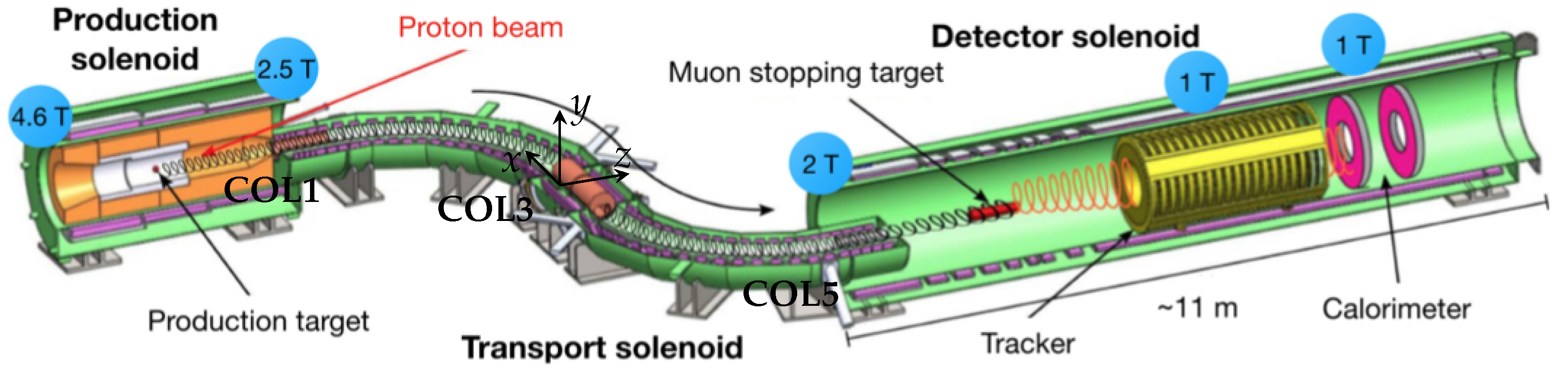
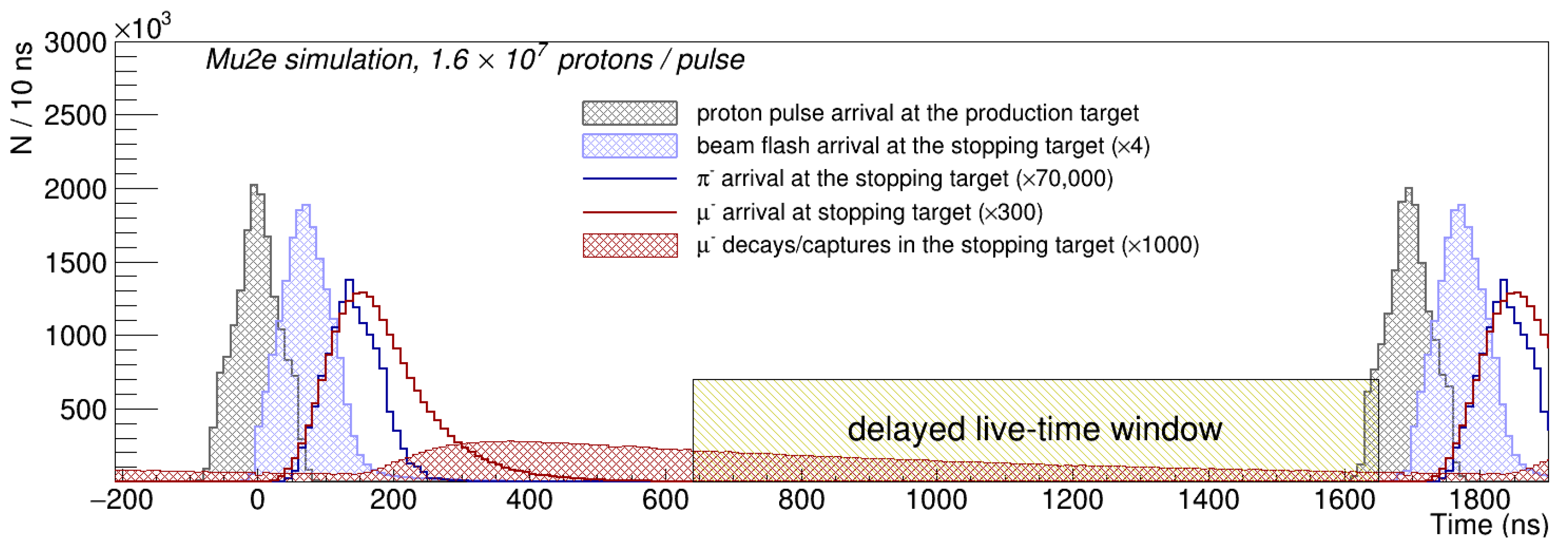
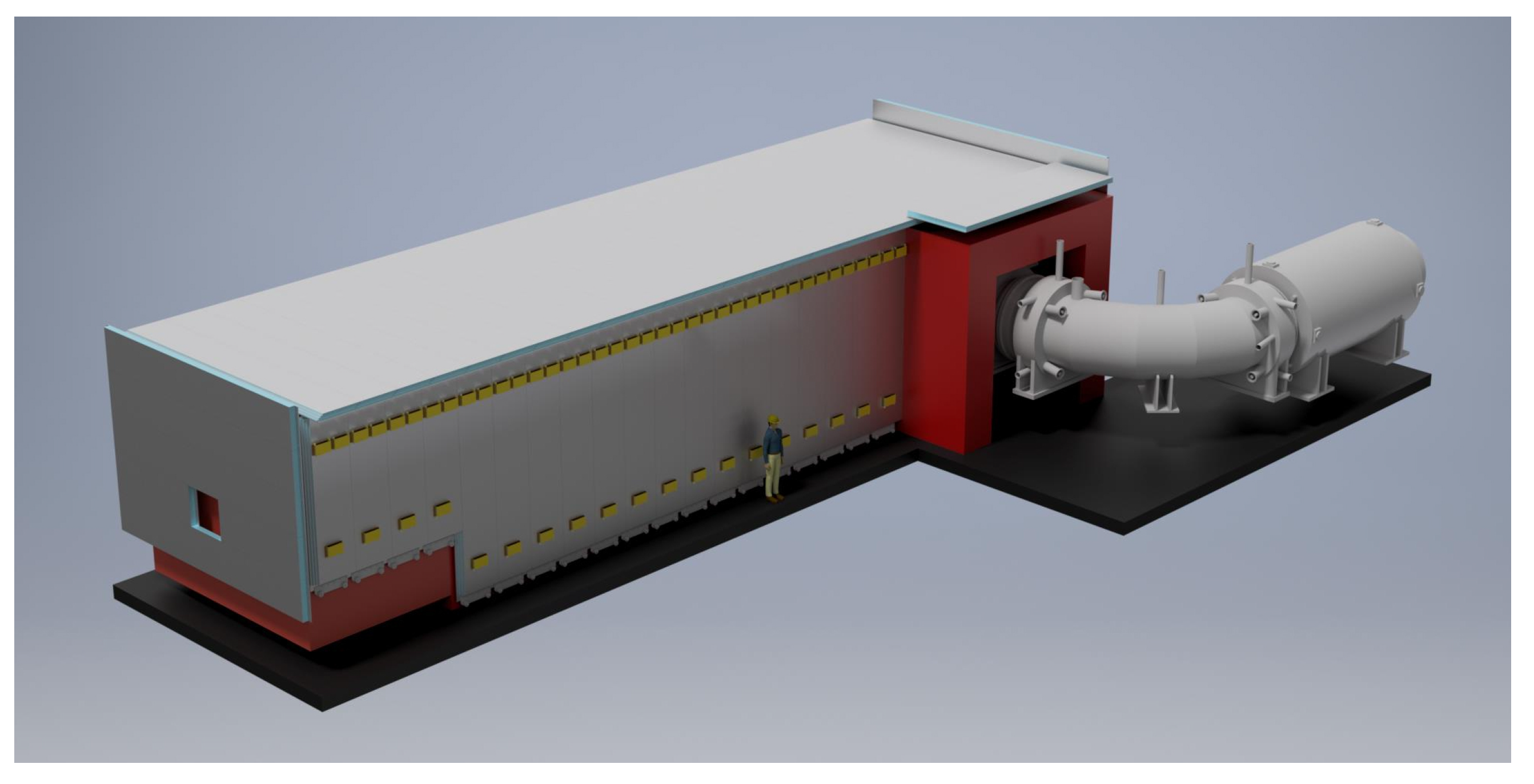
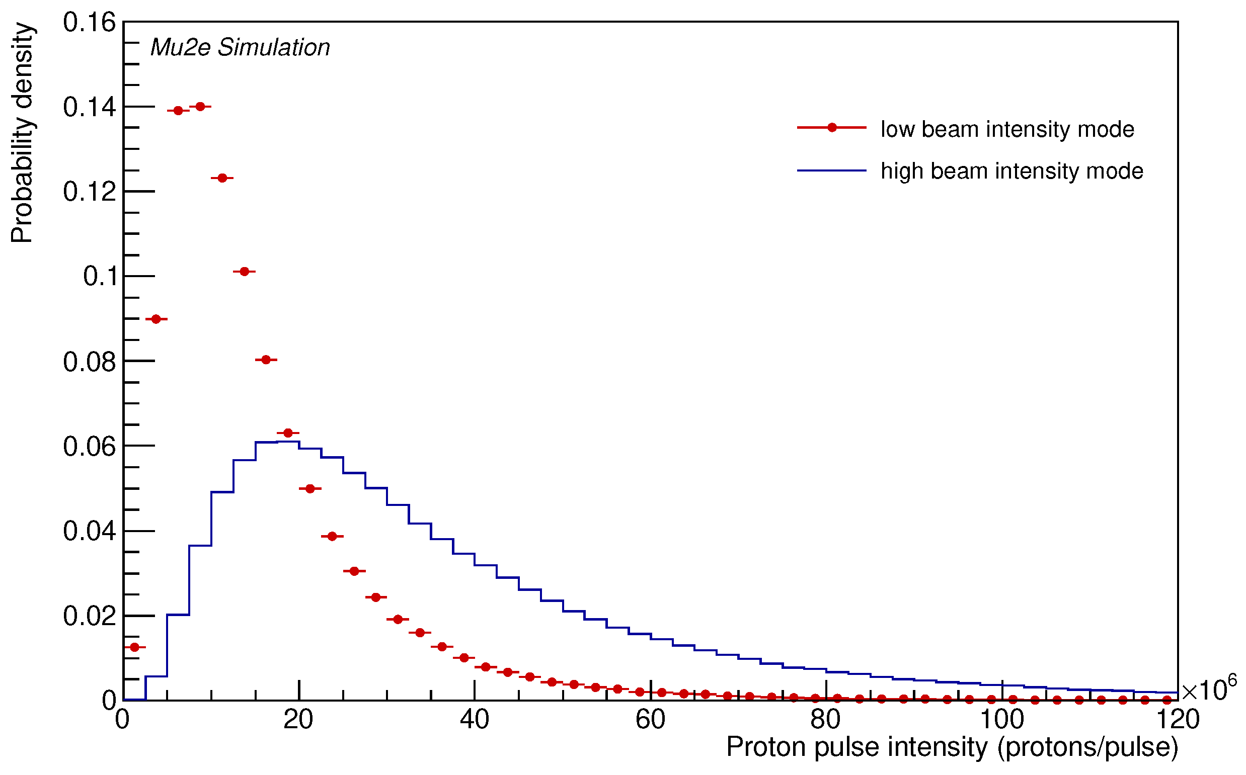
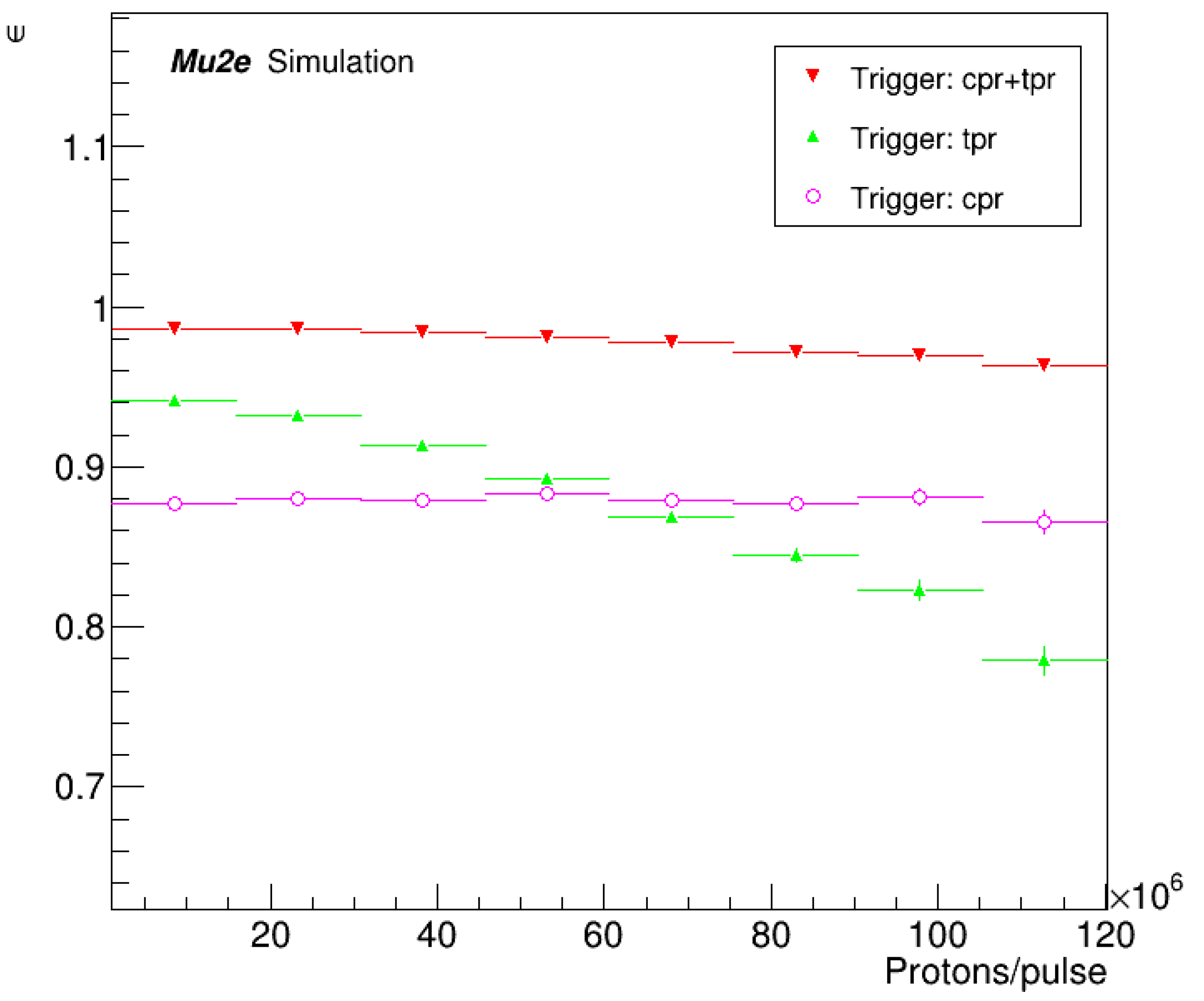
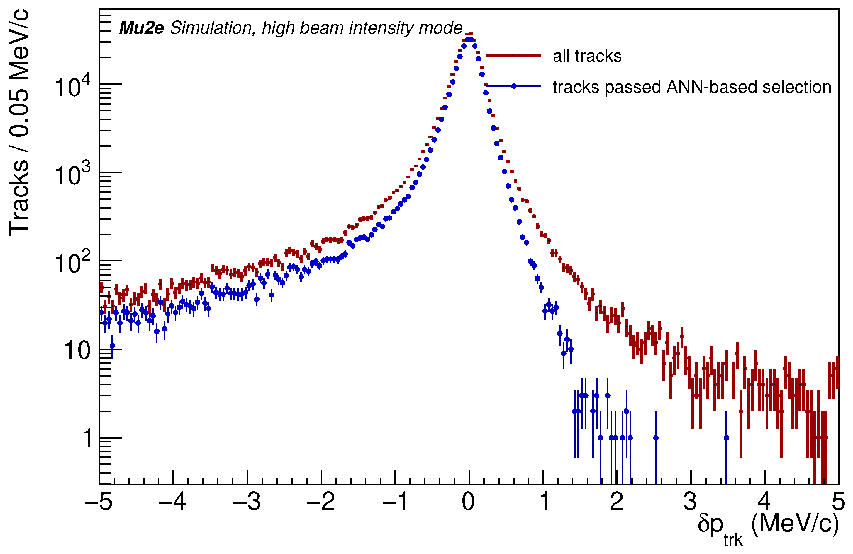
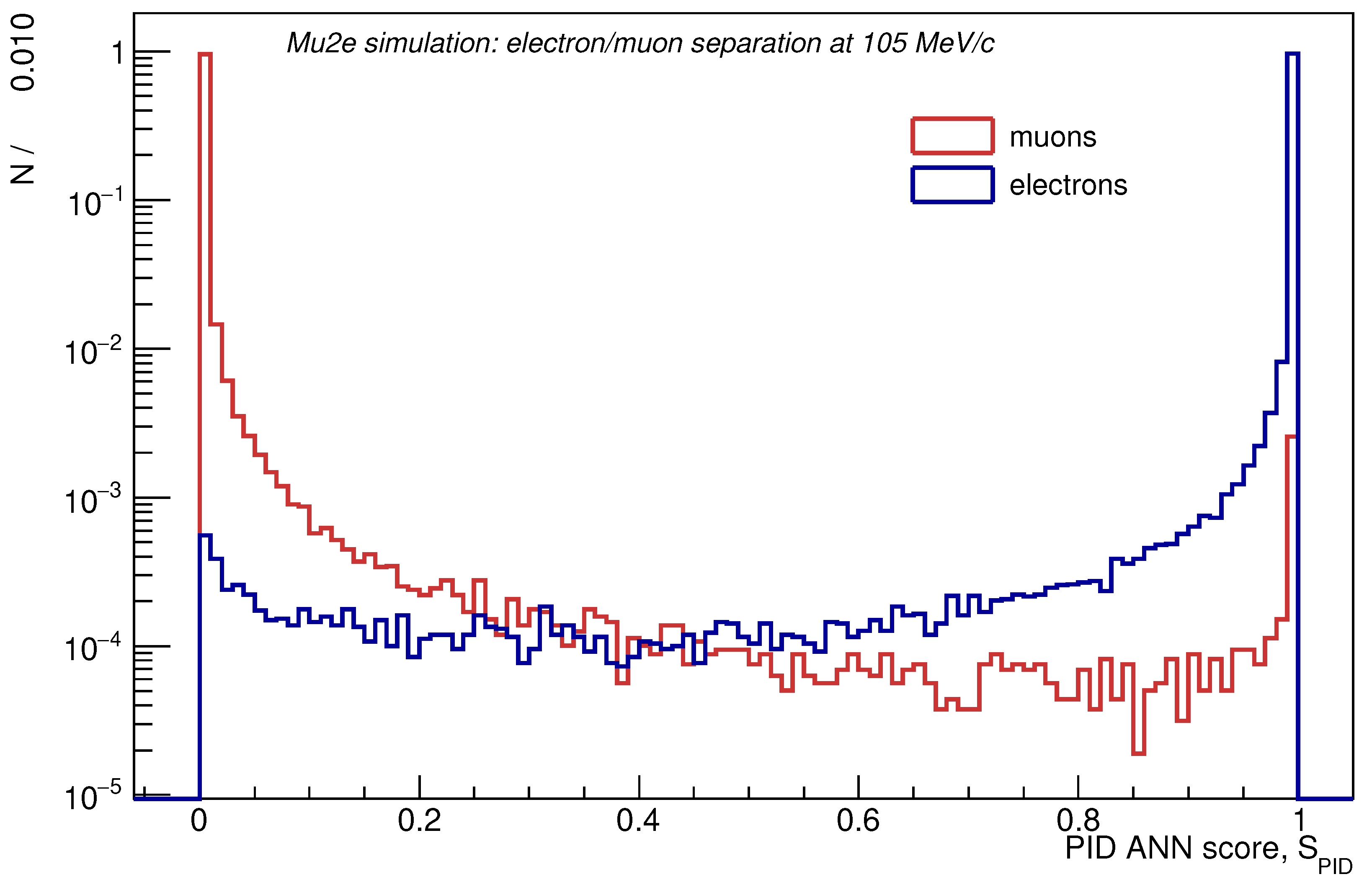
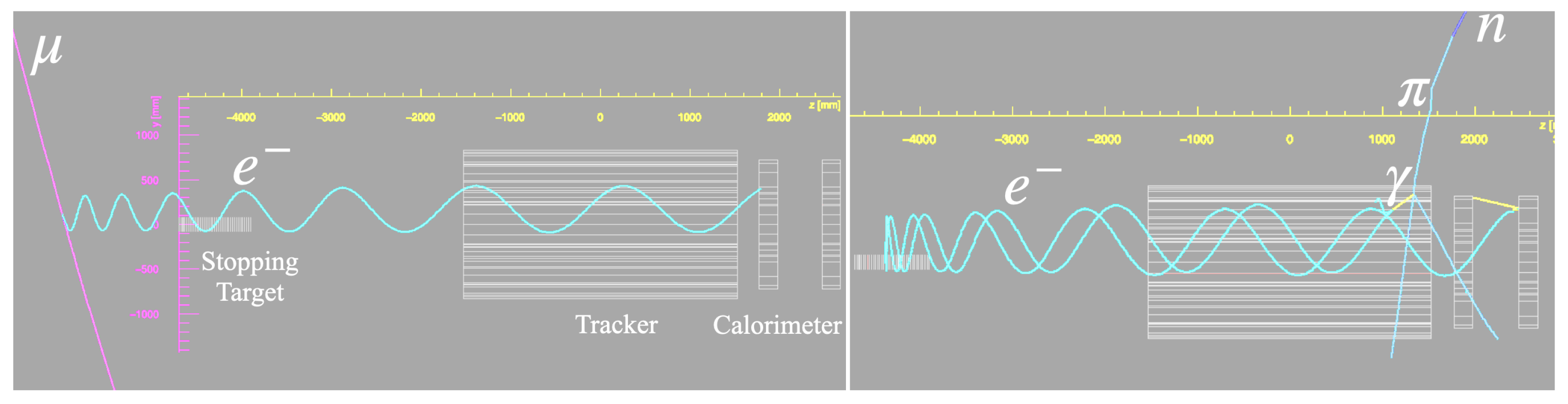
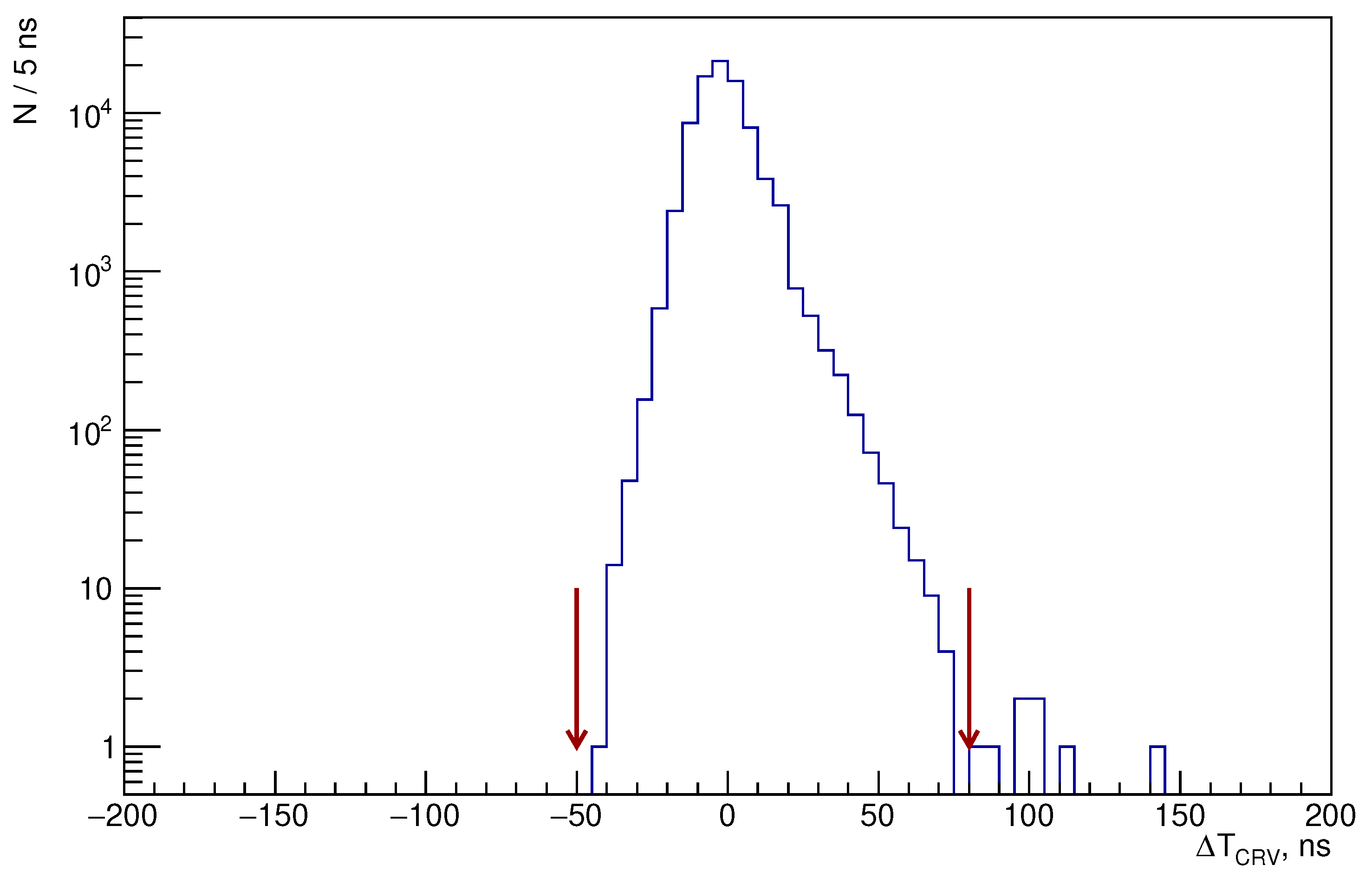
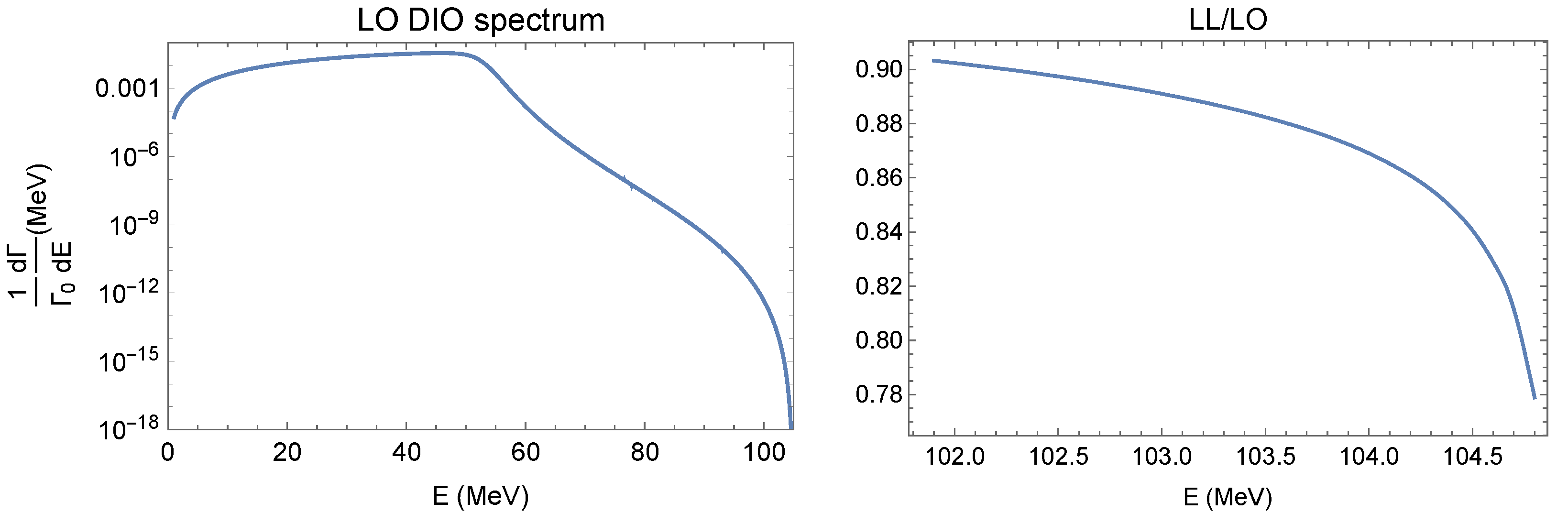
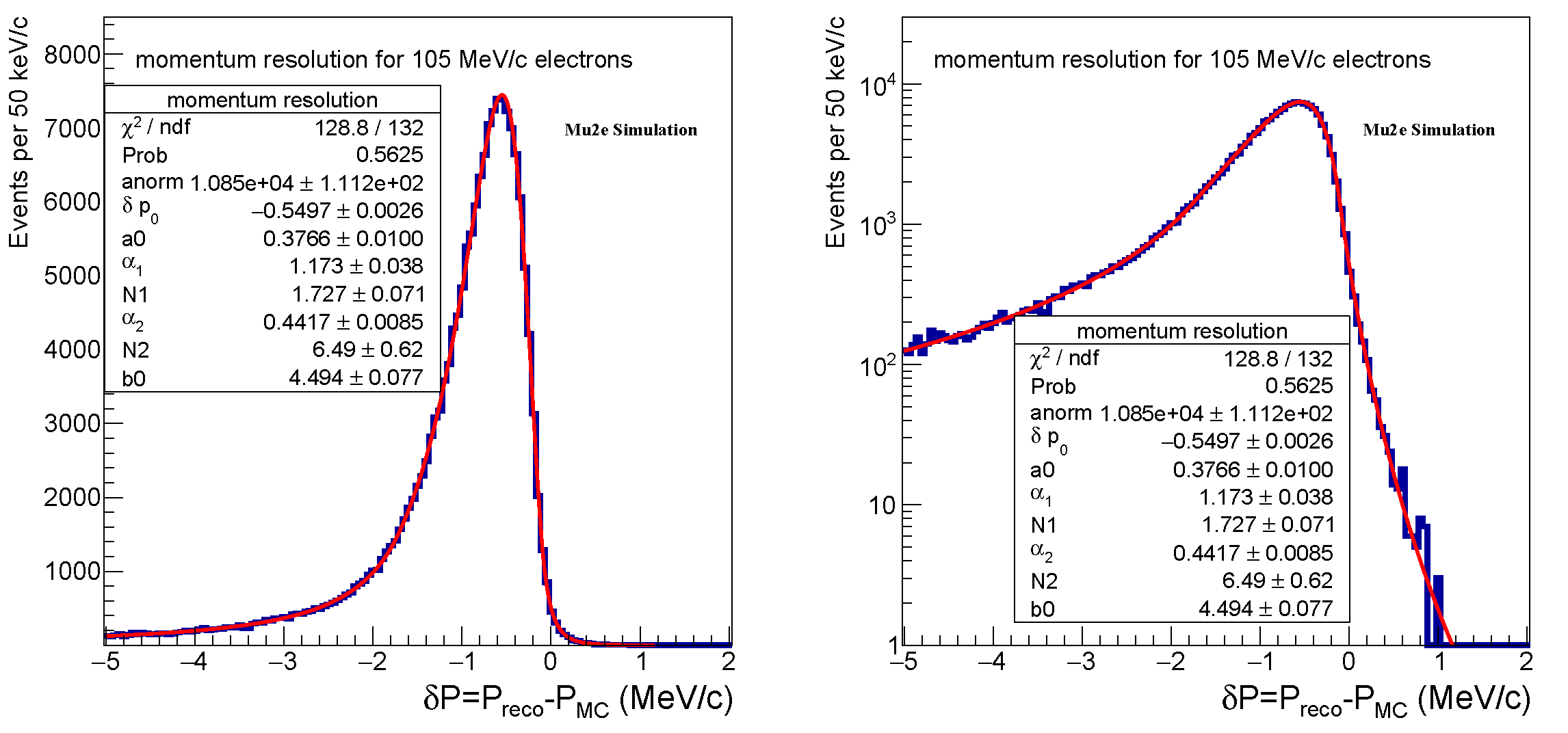
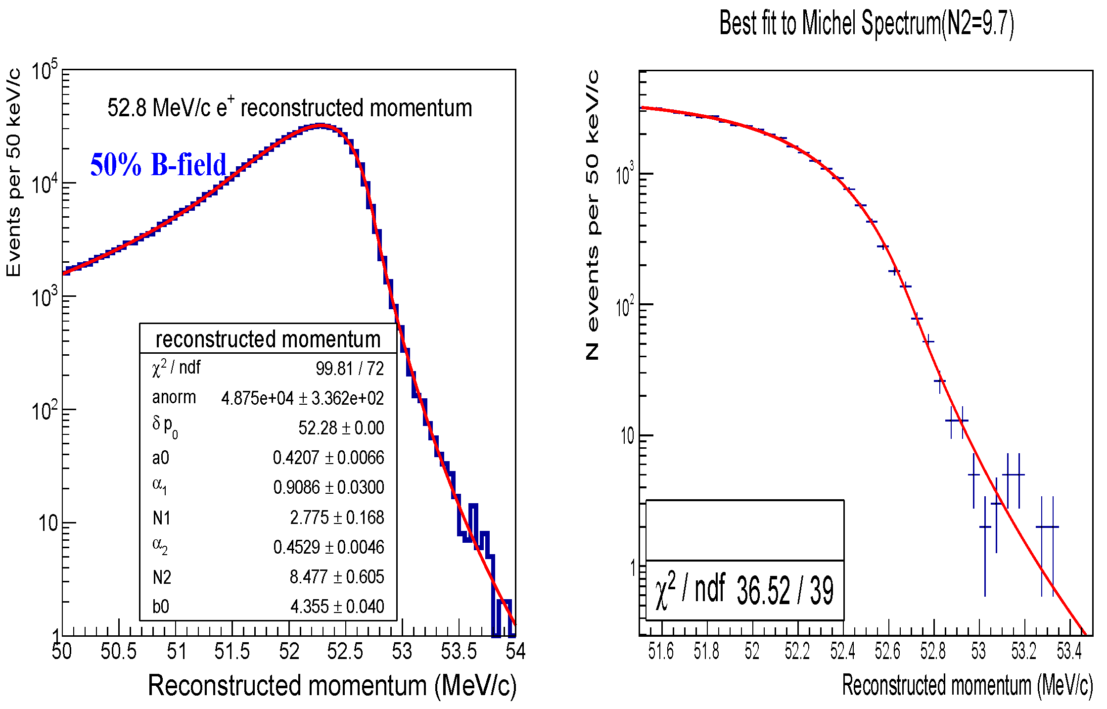
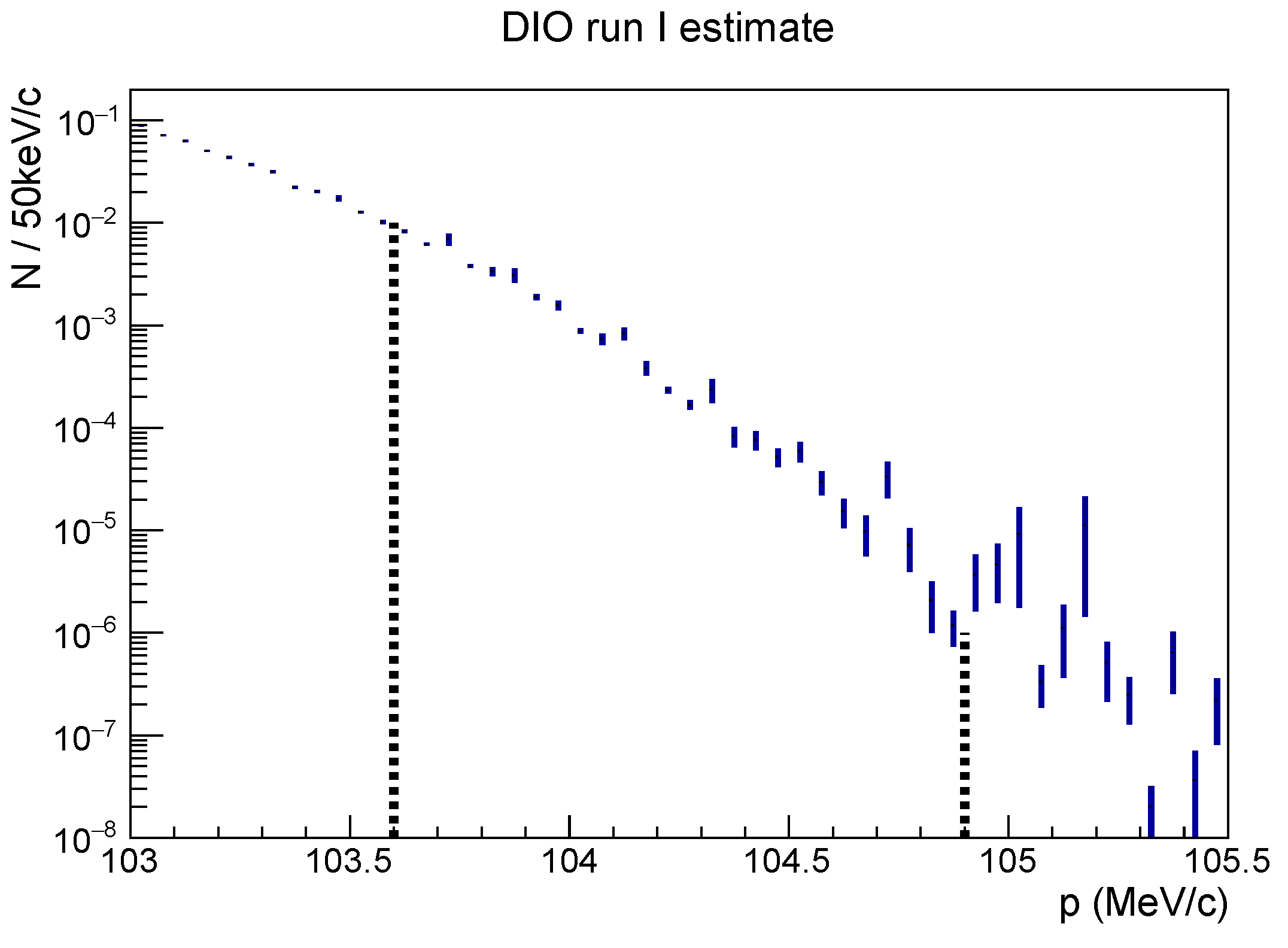
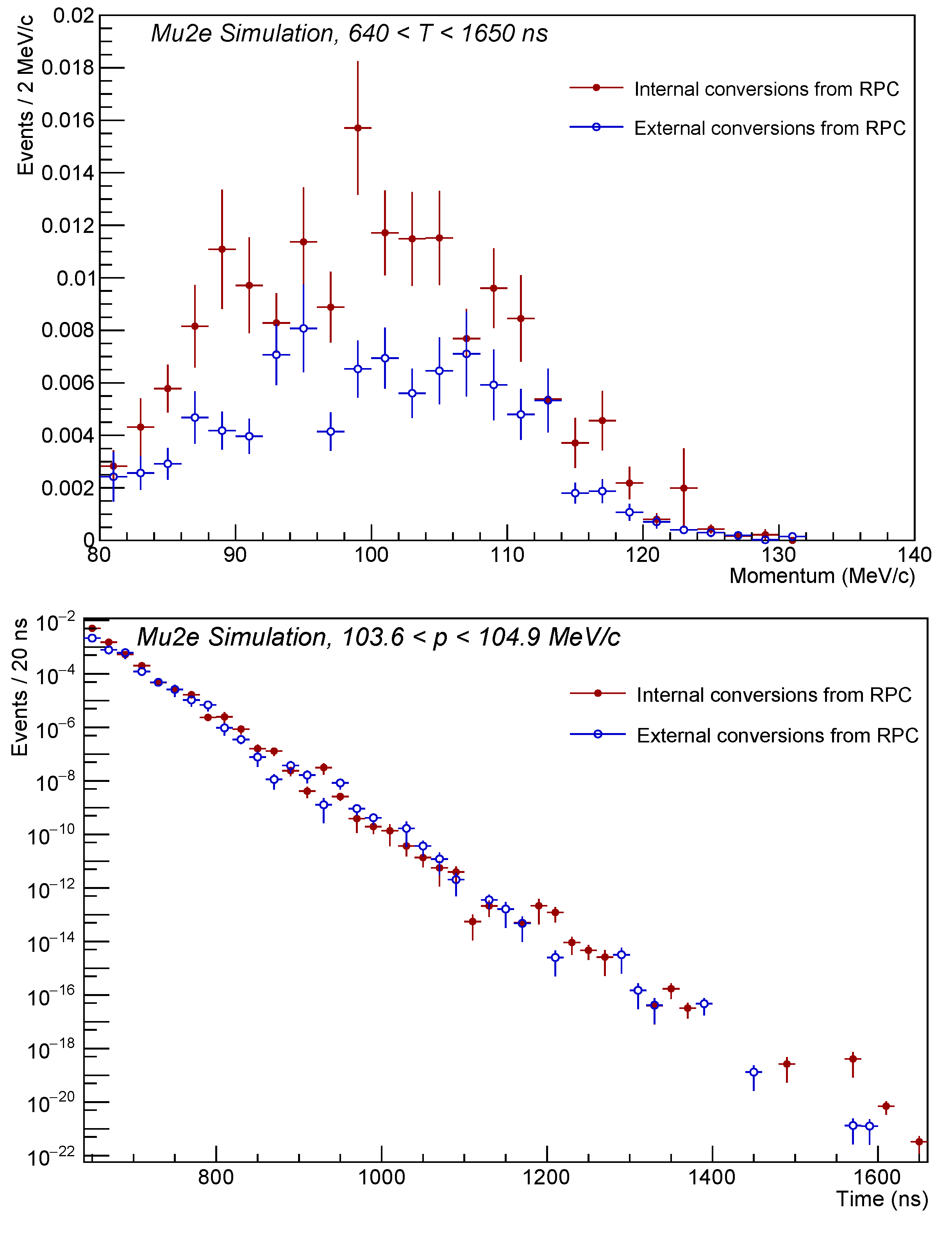
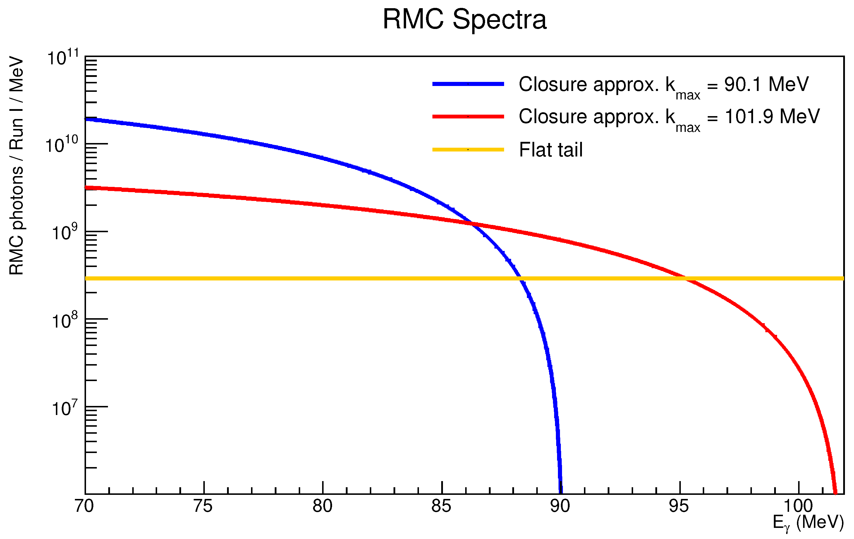
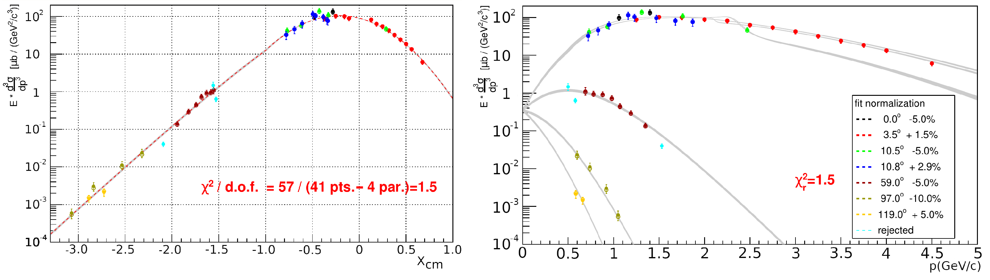
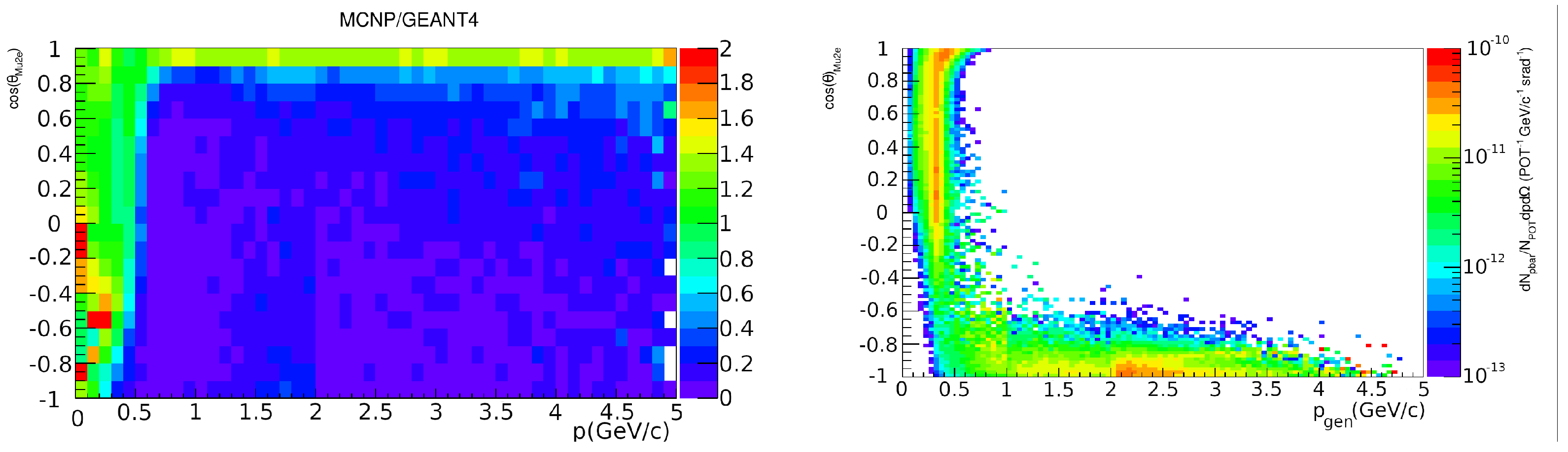
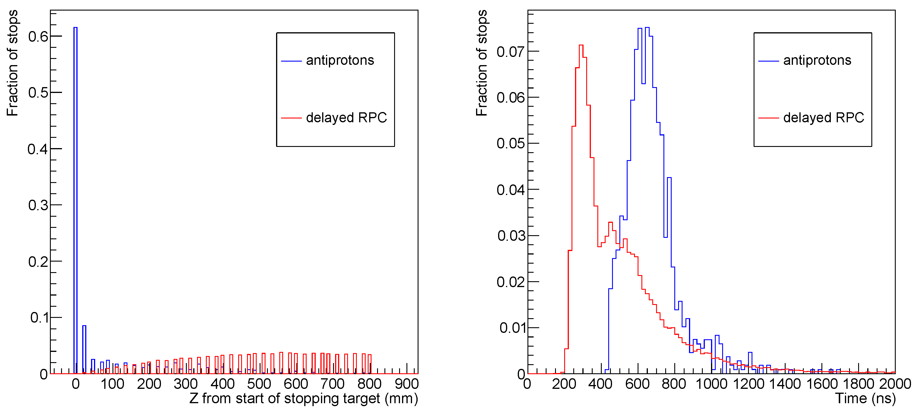
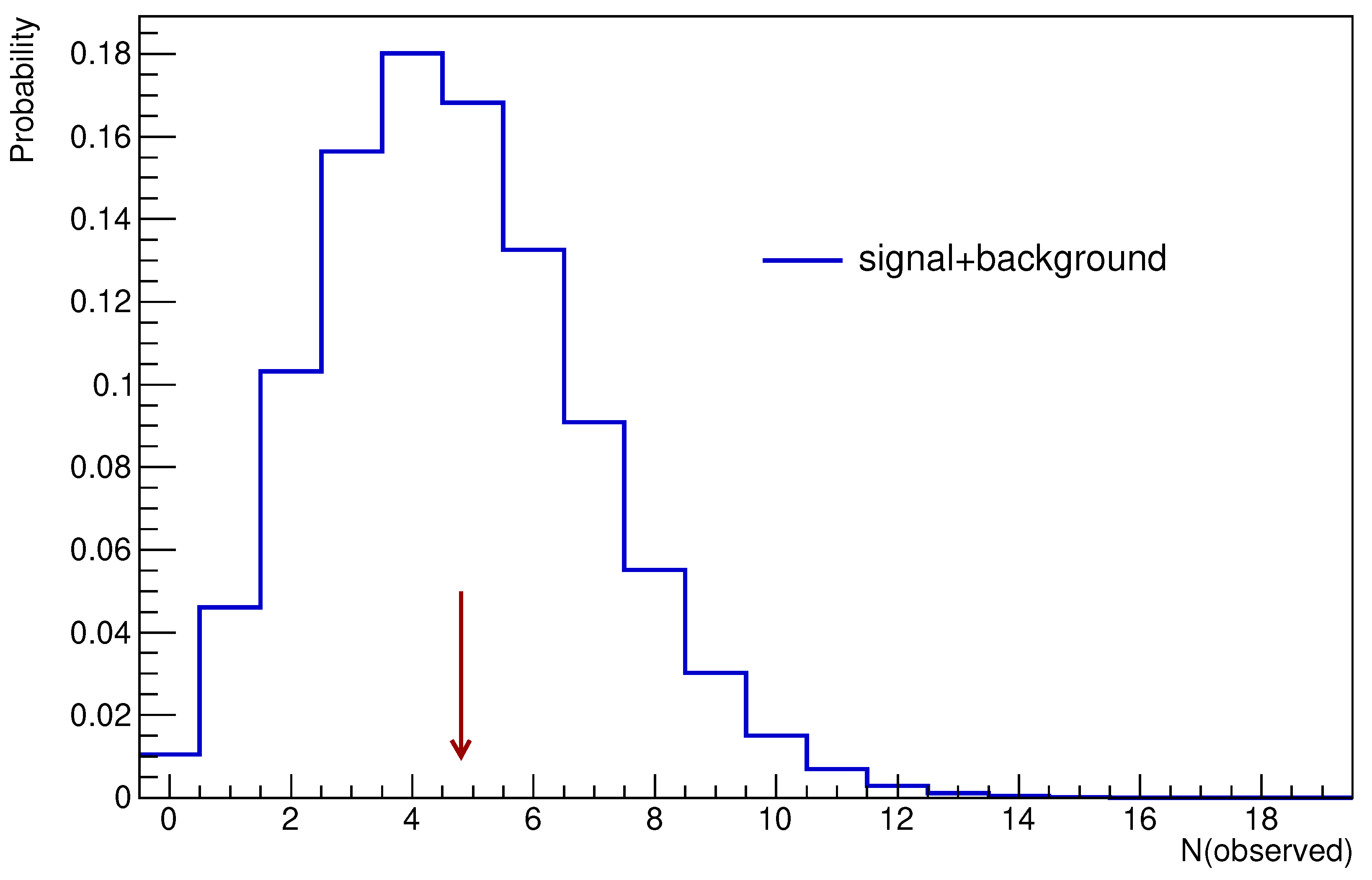
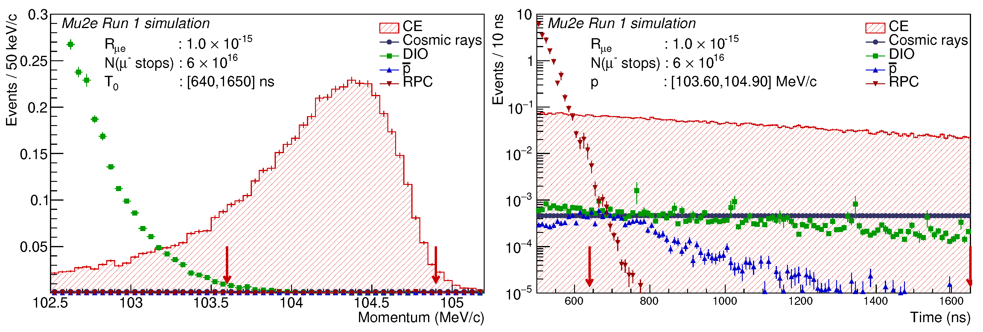
Table 1.
Expected running time, proton counts, and stopped muon counts for Mu2e Run I. The running time is the time, in seconds, during which the experiment is running and taking data. The numbers in the last two columns do not include the trigger, reconstruction, and selection efficiency.
Table 1.
Expected running time, proton counts, and stopped muon counts for Mu2e Run I. The running time is the time, in seconds, during which the experiment is running and taking data. The numbers in the last two columns do not include the trigger, reconstruction, and selection efficiency.
| Running Mode | Mean Proton Pulse Intensity | Running Time (s) | N (POT) | N (Stopped Muons) |
|---|---|---|---|---|
| Low intensity | ||||
| High intensity | ||||
| Total |
Table 2.
Breakdown of the DIO background relative systematic uncertainties.
| Source | Low Intensity Running Mode | High Intensity Running Mode | Run I Error |
|---|---|---|---|
| Momentum Scale | +62%,−38% | +50%,−34% | +59%,−37% |
| Theory | ± 2.5% | ±2.5% | ±2.5% |
| Total | +62%,−38% | +50%,−34% | +59%,−37% |
Table 3.
List of systematic uncertainties and their relative contributions to the RPC yield.
| Systematic Contribution | Internal Conversions | External Conversions |
|---|---|---|
| RPC fraction [46] | 9.3% | |
| Internal conversion coefficient [45] | 4.5% | |
| Pion production model | ||
| Total systematic uncertainty |
Table 4.
RMC background estimates using the altered closure approximations. These estimates use the optimized signal window introduced in Section 7, ns and . The estimates have a statistical accuracy of .
Table 4.
RMC background estimates using the altered closure approximations. These estimates use the optimized signal window introduced in Section 7, ns and . The estimates have a statistical accuracy of .
| RMC Tail Parameterization | Production Mechanism | Run I Background |
|---|---|---|
| Closure approx., = 101.9 MeV | On-shell | |
| Closure approx., = 101.9 MeV | Off-shell | |
| Flat | On-shell | |
| Flat | Off-shell |
Table 5.
Available data for antiproton production from proton interactions on different heavy nuclei. The antiproton momentum column () indicates the minimum and maximum measured momentum; when these are separated by a ÷ more than 2 points have been measured.
Table 5.
Available data for antiproton production from proton interactions on different heavy nuclei. The antiproton momentum column () indicates the minimum and maximum measured momentum; when these are separated by a ÷ more than 2 points have been measured.
| () | (, o) | () | Nuclear Target, Reference | |
|---|---|---|---|---|
| 2 | 10 | 0 | Tungsten, Anmann et al. [51] | |
| 13 | 10 | 3.5 | Tantalum, Sibirtsev et al. [52] | |
| 5 | 10 | 10.5 | Tantalum, Kiselev et al. [53] | |
| 8 | 10 | 10.8 | Gold, Barabash et al. [54] | |
| 8 | 10 | 59 | Tantalum, Kiselev et al. [53] | |
| 4 | 10 | 97 | Tantalum, Boyarinov et al. [55] | |
| 2 | 10 | 119 | Tantalum, Boyarinov et al. [55] |
Table 6.
Systematic uncertainties used in the sensitivity optimization procedure. The muon flux uncertainty is correlated between the signal and the DIO and RPC backgrounds.
Table 6.
Systematic uncertainties used in the sensitivity optimization procedure. The muon flux uncertainty is correlated between the signal and the DIO and RPC backgrounds.
| Parameter | Total Relative Uncertainty | Dominant Contribution |
|---|---|---|
| Signal acceptance | 4% | Momentum scale |
| Antiproton background | 100% | production cross section |
| Cosmic background | 20% | Cosmic flux normalization |
| DIO background | 59% | Momentum scale |
| RPC background | 29% | Pion production cross section |
| Muon flux | 10% | Flux measurement |
Table 7.
Summary of the sensitivity optimization. The sensitivity values are given with and without the inclusion of systematic uncertainties.
Table 7.
Summary of the sensitivity optimization. The sensitivity values are given with and without the inclusion of systematic uncertainties.
| Configuration | Discovery | (90% CL Limit) | N(Discovery Events) |
|---|---|---|---|
| No systematics | 5 | ||
| With systematics | 5 |
Table 8.
Background summary and SES using the optimized signal momentum and time window, and ns.
| Channel | Mu2e Run I |
|---|---|
| SES | |
| Cosmic rays | |
| DIO | |
| Antiprotons | |
| RPC in-time | |
| RPC out-of-time () | |
| RMC | |
| Decays in flight | |
| Beam electrons | |
| Total |
Disclaimer/Publisher’s Note: The statements, opinions and data contained in all publications are solely those of the individual author(s) and contributor(s) and not of MDPI and/or the editor(s). MDPI and/or the editor(s) disclaim responsibility for any injury to people or property resulting from any ideas, methods, instructions or products referred to in the content. |
© 2023 by the author. Licensee MDPI, Basel, Switzerland. This article is an open access article distributed under the terms and conditions of the Creative Commons Attribution (CC BY) license (https://creativecommons.org/licenses/by/4.0/).
Share and Cite
MDPI and ACS Style
Mu2e Collaboration. Mu2e Run I Sensitivity Projections for the Neutrinoless μ− → e− Conversion Search in Aluminum. Universe 2023, 9, 54. https://doi.org/10.3390/universe9010054
AMA Style
Mu2e Collaboration. Mu2e Run I Sensitivity Projections for the Neutrinoless μ− → e− Conversion Search in Aluminum. Universe. 2023; 9(1):54. https://doi.org/10.3390/universe9010054
Chicago/Turabian StyleMu2e Collaboration. 2023. "Mu2e Run I Sensitivity Projections for the Neutrinoless μ− → e− Conversion Search in Aluminum" Universe 9, no. 1: 54. https://doi.org/10.3390/universe9010054
Note that from the first issue of 2016, this journal uses article numbers instead of page numbers. See further details here.