
On the Degeneracy between fσ8 Tension and Its Gaussian Process Forecasting


1
Laboratory of Astrophysics, Institute of Physics, École Polytechnique Fédérale de Lausanne, 1290 Versoix, Switzerland
2
Instituto de Ciencias Nucleares, Universidad Nacional Autónoma de México, Circuito Exterior C.U., A.P. 70-543, México 04510, Mexico
*
Author to whom correspondence should be addressed.
†
These authors contributed equally to this work.
Universe 2022, 8(8), 394; https://doi.org/10.3390/universe8080394
Submission received: 21 June 2022
/
Revised: 20 July 2022
/
Accepted: 25 July 2022
/
Published: 27 July 2022
(This article belongs to the Special Issue Frontiers in Numerical Precision: From Astrophysics to Cosmology)
Abstract
:In this Article, we reconstruct the growth and evolution of the cosmic structure of the Universe using Markov chain Monte Carlo algorithms for Gaussian processes. We estimate the difference between the reconstructions that are calculated through a maximization of the kernel hyperparameters and those that are obtained with a complete exploration of the parameter space. We find that the difference between these two approaches is of the order of . Furthermore, we compare our results with those obtained by Planck Collaboration 2018 assuming a CDM model and we do not find a statistically significant difference in the redshift range where the reconstructions of have been made.
1. Introduction
Currently, the estimates of the value of , obtained from the CDM fit to the cosmic microwave background (CMB) differ between 2–3 with respect to the value of obtained with the analysis of galaxy clustering using two-point correlation functions (2PCFs) [1]. This discrepancy is the so-called tension [2,3]. Additionally, the most recent estimate of the value of the Hubble constant, , obtained with the calibration of the cosmic distance ladder scale through Cepheid stars and supernovae type Ia is different [4] from the value CDM obtained with CMB observations.
Specifically, the primary anisotropies of the CMB exhibit a tension in the matter clustering strength at the level of 2–3 when compared to lower z probes such as weak gravitational lensing and galaxy clustering (e.g., [1,5,6,7,8,9,10,11,12,13]). The lower z probes (see Figure 4 from [14]) select a lower value of compared to the high z CMB estimates. The measured value is model-dependent and in the majority of the scenarios it is considered a standard flat CDM model. Of course, this latter model provides a good fit to the data from all probes but predicts a lower value of structure formation compared to what we expect from the CMB [6]. In [14], it is reported the latter parameter estimates and constraints, where we notice that there might be slight differences in the selection that enters each study. For example, on one hand, a statistical property of the distribution might be selected, such as its mean or mode together with the asymmetric C.L around this value or the standard deviation of the data points. On the other hand, the statistics to the full posterior distribution can be adopted, such as the maximum a posteriori point or the best-fitting values and their errors. In any case, these considerations can affect the estimated values of the parameters, in particular when the posterior distributions are significantly non-Gaussian.
Many models beyond CDM models have been proposed as tentative explanations to this observed tension; however, a nonspecific model has been proven much better than the standard one. In such a case, we should look for a reason why the tension between the CMB and cosmic shear in the inferred value of can arise from unaccounted baryonic physics, other unknown systematic errors or a statistical fluke. Furthermore, we require that be independent of the CMB and cosmic shear. In this matter, the redshift-space distortion (RSD) data also prefer a small value of , that is 2–3 lower than the Planck result [15]. However, the RSD values on are sensitive to the cosmological model.
In this paper, we perform the reconstructions of the observations using Gaussian processes (GP) to analyze if the reconstructions suggest possible deviations with respect to the standard cosmological model. Unlike previous studies [16,17,18], we take into account the Planck 2018 confidence contours when comparing the predictions of CDM with those of the reconstructions. This allows us to control the statistical uncertainties. The possibility of using GP to distinguish between modified gravity (MG) and general relativity (GR) has been analyzed [19], e.g., by treating the perturbations of a disformally scalar field model whose background mimics the CDM [20].
Previous articles [17] have used the reconstructions of the Hubble parameter to reconstruct and to show how different values of change the value of the tension. However, the large number of free parameters associated with that approach leads to large uncertainties on the reconstructions, which could explain why a ∼4 change in the value of only causes a ∼1 change in the value of the tension.
Unlike the standard way to reconstruct [17], in this work, we reconstruct (z) by directly using the estimations of , therefore it is possible to remove and as free parameters and reduce the uncertainty in the confidence contours. However, we should mention that our approach does not allow us to obtain a direct estimate of the aforementioned parameters.
In this line of thought, several numerical methods have been developed over the years, showing a great advance in the precision cosmology road, e.g., methods that involves artificial neural network (ANN) to reconstruct late–time cosmology data [21], the creation of mock datasets through machine learning (ML) based on the LSST survey and using a fiducial cosmology [22] and Bayesian analyses in order to reassess the discrepancy between the CMB and weak lensing data [15].
Furthermore, we analyze two different approaches to obtain the value of the confidence contours of the reconstructions. The first approach consists in the maximization of the likelihood associated with the GP in order to obtain the value of the free parameters from the reconstruction. This approach has been frequently used in the literature to perform GP in the context of cosmology [17,19,23,24,25]; however, in some works [26,27], it has been shown that this process could lead to an underestimation of the confidence contours of the reconstructions. The second approach consists in an exploration of the parameter space of the free parameters through Markov chain Monte Carlo (MCMC) methods [28]. This method allows us to obtain an estimate of the uncertainties associated with each parameter, which contributes to solve the underestimation problem.
1.1. Treatment of Data Samples and Methodology
To use the GP method, we need to assume that our set of observations “” given in the set of redshifts “” is Gaussian distributed around the underlying function that we seek to reconstruct, g(z). This allows us to associate a probability distribution with the data:
where is the mean value of the observations, C is its covariance matrix and K is the covariance matrix associated with the Gaussian processes also known as the kernel function. It can be shown that the mean value and covariance matrix of the reconstructed function in the set of redshifts are given by [26].
The measurements of the clustering pattern of matter in the redshift space allow us to infer parameters such as the linear growth of matter perturbations and the variance of matter fluctuations on a given scale R. The variance is usually reported on a scale Mpc, that is, .
However, an exact determination of the value of turns out to be complex, since the galaxy redshift surveys provide an estimate of the perturbations in terms of galaxy densities instead of directly in terms of matter density . Unfortunately, the exact value of the parameter b remains uncertain [29]; for that reason, the measurements are reported in terms of , since it is independent of the parameter b [17].
To perform the reconstructions we used the compilation of measurements of shown in Table 1 of [30]. This table contains 30 measurements of , together with their uncertainties and their covariance matrices.
According to the latter, the inferred values of depend on two things: (i) the anisotropies in the power spectrum of the peculiar velocities of galaxies and (ii) the fiducial cosmology chosen to estimate the values of . If the cosmology chosen to perform the data analysis does not adequately describe the geometry of the universe, then nontrivial anisotropies are introduced in the 2PCFs, which are directly correlated with the estimated value of ; this effect is known as Alcock–Paczynski (AP) effect. It is important to note that the values sometimes are reported assuming [31] different fiducial cosmologies, e.g.,
1.2. Alcock-Paczynski Corrections
If the reconstructions are performed without including corrections to the AP effect, then all the information from different fiducial cosmologies are mixed, i.e., it is not possible to properly estimate the tension between the reconstructions and the CDM model. We applied the correction to the AP effect given in [31], whose corrections state that if a measurement of has been obtained assuming a fiducial cosmology with a Hubble parameter and angular diameter , then the corresponding value of assuming a different fiducial cosmology with and can be approximated as:
To correct the AP effect, we considered a vanilla CDM cosmology with the parameters inferred from the Planck 2018 Collaboration [34], such that the high redshift data from Planck TT, TE, EE + lowE are . Combining these data with secondary CMB anisotropies, in the form of CMB lensing, serves to tighten the constraint to .
To proceed with this calculation, we set the following steps:
- Suppose that and are two measurements of that were obtained assuming the fiducial cosmologywith , the mean value of each measurement, , their 1 uncertainties and also suppose that the measurements are correlated through a covariance matrix C
1.3. Kernel Metrics
It has been shown that the kernel chosen to perform the reconstructions can affect the uncertainties of the parameters derived from the reconstructions [26,27,36]. In particular, the Gaussian kernel can lead to uncertainties up to three times smaller than the value of the uncertainties obtained with the Matérn covariance functions [37]. Since this could be associated with the problem of underestimation of uncertainties, we chose to use only Matérn kernels, specifically the Matérn 3/2 and Matérn 5/2 kernels. These covariance functions have been used, e.g., in studies that analyze how the choice between different kernels affect the value of that is obtained from the reconstructions of the cosmic late expansion [36] and in an analysis on how different kernels can affect the constraints on modified theories of gravity [23]. The Matérn 3/2 and Matérn 5/2 kernels are, respectively, defined as:
where and l are free parameters that measure the width of the reconstructed function and the correlation between the function evaluated at two given points and . With these kernels at hand, we are ready to proceed with two different methods to obtain the value of the hyperparameters of the kernel:
- Method (i) consists in the maximization of the likelihood associated with the observations Equation (1).
- Method (ii) consists in a full exploration of the parameter space for the hyperparameters through MCMC methods. This approach is convenient when the parameter space is multidimensional, and it could help us to find the true maximum likelihood estimate in cases where the algorithm for maximization gets stuck in a local minima.
Since is a squared quantity in both covariance Functions (9) and (10), if (, ) are the values of the hyperparameters that maximize Equation (1), then (, ) also maximize Equation (1), and this leads to a bimodal posterior distribution for the hyperparameter . Since with one mode, we can obtain the full information to carry out the reconstructions, it is convenient to establish priors that only take into account the positive (or negative) branch of the parameter space for . With this method, it is possible to reduce the computational time required to calculate the posterior distribution of the hyperparameters and it also allows us to avoid convergence problems within the numerical code.
Notice that covariance Functions (9) and (10) are not symmetric on l. However, we expected positive values of l, otherwise the correlation between the points , would grow proportionally to
Since hyperparameters were restricted to be positive, we considered for them gamma probability distributions as priors. The probability density function for a random variable X that follows a gamma distribution with parameters and is given by
with the gamma function. The mean value of is , the mode is and the variance is Var [35]. In order to find the value of the hyperparameters of the covariance functions that maximizes Equation (1), we performed a maximum likelihood estimation (MLS) with the code [26], and afterwards, we proceeded with a standard MCMC analysis using the publicly available code PyMC3 [38]. For both hyperparameters, we chose gamma priors with and equal to their MLS. We estimated the convergence of the chains using a Gelman–Rubin convergence criterion [39] with . The reconstructions were estimated with two different approaches: (1) we used the mean value of the hyperparameters to estimate the mean value of the reconstructions and (2) we used the mode. Our results are detailed in Table 1 and Table 2 and in Figure 1 and Figure 2.
In order to distinguish between reconstructions, we defined the tension metric as follows:
where and are the mean values of the reconstructions and , respectively. and are the statistical uncertainties. Notice that Equation (13) quantifies the difference in standard deviations between the reconstructions and .
From Table 3 and Table 4, we can notice that for both kernels the tension for all methods is of the order of 2 in the observable redshift region. The mean value of the reconstructions obtained through the different methods represent of its total value.
Additionally, to test the performance of each model describing by the observations, we estimated the chi-square statistics as follows
with the inverse of the covariance matrix of the data. The results are shown in Table 5 and Table 6. With these results and with those obtained using the function, we conclude that there is no statistically significant difference between CDM and the reconstructions presented here (see Table 5 and Table 6).
2. Conclusions
In this Article, we reconstructed the observations using two different kernels and three different methods to obtain the value of the hyperparameters. The tension between CDM and the reconstructions did not give values above 2.2. We showed that choosing different kernels led to differences of the order of ∼0.1 in the value of the tension. Furthermore, we also showed that the change in the value of the tension obtained with different methods (with the kernel fixed) was also of the order of . Therefore, we conclude that there is no significant statistical difference between the predictions given for by CDM with Planck 2018 parameters and those given by the reconstructions, since the maximum tension between both was below .
Author Contributions
Writing—review & editing, M.R. and C.E.-R. All authors have read and agreed to the published version of the manuscript.
Funding
MC acknowledges support from the European Research Council (ERC) under the European Union’s Horizon 2020 research and innovation programme (grant agreement no. 947660).
Data Availability Statement
Not applicable.
Acknowledgments
CE-R is supported by DGAPA-PAPIIT UNAM Project TA100122 and acknowledges the Royal Astronomical Society as FRAS 10147. This work is part of the Cosmostatistics National Group (https://www.nucleares.unam.mx/CosmoNag/index.html (CosmoNag)) Saturday. 24 July 2022. project. The authors would like to acknowledge the PyMC3 and Arviz communities for their helpful recommendations on the modified version of the arviz code [40].
Conflicts of Interest
The authors declare no conflict of interest.
References
- Abbott, T.M.C.; Aguena, M.; Alarcon, A.; Allam, S.; Alves, O.; Amon, A.; Andrade-Oliveira, F.; Annis, J.; Avila, S.; Bacon, D.; et al. Dark Energy Survey Year 3 results: Cosmological constraints from galaxy clustering and weak lensing. Phys. Rev. D 2022, 105, 023520. [Google Scholar] [CrossRef]
- Tröster, T.; Sánchez, A.G.; Asgari, M.; Blake, C.; Crocce, M.; Heymans, C.; Hildebrandt, H.; Joachimi, B.; Joudaki, S.; Kannawadi, A.; et al. Cosmology from large-scale structure: Constraining ΛCDM with BOSS. Astron. Astrophys. 2020, 633, L10. [Google Scholar] [CrossRef] [Green Version]
- Di Valentino, E.; Anchordoqui, L.A.; Akarsu, Ö.; Ali-Haimoud, Y.; Amendola, L.; Arendse, N.; Asgari, M.; Ballardini, M.; Basilakos, S.; Battistelli, E.; et al. Cosmology Intertwined III: fσ8 and S8. Astropart. Phys. 2021, 131, 102604. [Google Scholar] [CrossRef]
- Riess, A.G.; Yuan, W.; Macri, L.M.; Scolnic, D.; Brout, D.; Casertano, S.; Jones, D.O.; Murakami, Y.; Breuval, L.; Brink, T.G.; et al. A Comprehensive Measurement of the Local Value of the Hubble Constant with 1 km/s/Mpc Uncertainty from the Hubble Space Telescope and the SH0ES Team. arXiv 2021, arXiv:2112.04510. [Google Scholar] [CrossRef]
- Asgari, M.; Tröster, T.; Heymans, C.; Hildebrandt, H.; Van den Busch, J.L.; Wright, A.H.; Choi, A.; Erben, T.; Joachimi, B.; Joudaki, S.; et al. KiDS+VIKING-450 and DES-Y1 combined: Mitigating baryon feedback uncertainty with COSEBIs. Astron. Astrophys. 2020, 634, A127. [Google Scholar] [CrossRef]
- Asgari, M.; Lin, C.-A.; Joachimi, B.; Giblin, B.; Heymans, C.; Hildebrandt, H.; Kannawadi, A.; Stölzner, B.; Tröster, T.; van den Busch, J.L.; et al. KiDS-1000 Cosmology: Cosmic shear constraints and comparison between two point statistics. Astron. Astrophys. 2021, 645, A104. [Google Scholar] [CrossRef]
- Joudaki, S.; Hildebrandt, H.; Traykova, D.; Chisari, N.E.; Heymans, C.; Kannawadi, A.; Kuijken, K.; Wright, A.H.; Asgari, M.; Erben, T.; et al. KiDS+VIKING-450 and DES-Y1 combined: Cosmology with cosmic shear. Astron. Astrophys. 2020, 638, L1. [Google Scholar] [CrossRef]
- Amon, A.; Gruen, D.; Troxel, M.A.; MacCrann, N.; Dodelson, S.; Choi, A.; Doux, C.; Secco, L.F.; Samuroff, S.; Krause, E.; et al. Dark Energy Survey Year 3 results: Cosmology from cosmic shear and robustness to data calibration. Phys. Rev. D 2022, 105, 023514. [Google Scholar] [CrossRef]
- Secco, L.F.; Samuroff, S.; Krause, E.; Jain, B.; Blazek, J.; Raveri, M.; Campos, A.; Amon, A.; Chen, A.; Doux, C.; et al. Dark Energy Survey Year 3 results: Cosmology from cosmic shear and robustness to modeling uncertainty. Phys. Rev. D 2022, 105, 023515. [Google Scholar] [CrossRef]
- Loureiro, A.; Whittaker, L.; Mancini, A.S.; Joachimi, B.; Cuceu, A.; Asgari, M.; Stölzner, B.; Tröster, T.; Wright, A.H.; Bilicki, M.; et al. KiDS & Euclid: Cosmological implications of a pseudo angular power spectrum analysis of KiDS-1000 cosmic shear tomography. arXiv 2021, arXiv:2110.06947. [Google Scholar]
- Hildebrandt, H.; Köhlinger, F.; Van den Busch, J.L.; Joachimi, B.; Heymans, C.; Kannawadi, A.; Wright, A.H.; Asgari, M.; Blake, C.; Hoekstra, H.; et al. KiDS+VIKING-450: Cosmic shear tomography with optical and infrared data. Astron. Astrophys. 2020, 633, A69. [Google Scholar] [CrossRef]
- Abbott, T.M.C.; Aguena, M.; Alarcon, A.; Allam, S.; Allen, S.; Annis, J.; Avila, S.; Bacon, D.; Bechtol, K.; Bermeo, A.; et al. Dark Energy Survey Year 1 Results: Cosmological constraints from cluster abundances and weak lensing. Phys. Rev. D 2020, 102, 023509. [Google Scholar] [CrossRef]
- Philcox, O.H.E.; Ivanov, M.M. BOSS DR12 full-shape cosmology: ΛCDM constraints from the large-scale galaxy power spectrum and bispectrum monopole. Phys. Rev. D 2022, 105, 043517. [Google Scholar] [CrossRef]
- Abdalla, E.; Abellán, G.F.; Aboubrahim, A.; Agnello, A.; Akarsu, Ö.; Akrami, Y.; Alestas, G.; Aloni, D.; Amendola, L.; Anchordoqui, L.A.; et al. Cosmology intertwined: A review of the particle physics, astrophysics, and cosmology associated with the cosmological tensions and anomalies. J. High Energy Astrophys. 2022, 34, 49–211. [Google Scholar] [CrossRef]
- Nunes, R.C.; Vagnozzi, S. Arbitrating the S8 discrepancy with growth rate measurements from redshift-space distortions. Mon. Not. Roy. Astron. Soc. 2021, 505, 5427. [Google Scholar] [CrossRef]
- Benisty, D. Quantifying the S8 tension with the Redshift Space Distortion data set. Phys. Dark Univ. 2021, 31, 100766. [Google Scholar] [CrossRef]
- Li, E.K.; Du, M.; Zhou, Z.H.; Zhang, H.; Xu, L. Testing the effect of H0 on fσ8 tension using a Gaussian process method. Mon. Not. Roy. Astron. Soc. 2021, 501, 4452–4463. [Google Scholar] [CrossRef]
- Said, J.L.; Mifsud, J.; Sultana, J.; Adami, K.Z. Reconstructing teleparallel gravity with cosmic structure growth and expansion rate data. J. Cosmol. Astropart. Phys. 2021, 6, 015. [Google Scholar] [CrossRef]
- Reyes, M.; Escamilla-Rivera, C. Improving data-driven model-independent reconstructions and updated constraints on dark energy models from Horndeski cosmology. J. Cosmol. Astropart. Phys. 2021, 7, 048. [Google Scholar] [CrossRef]
- Dusoye, A.; de la Cruz-Dombriz, A.; Dunsby, P.; Nunes, N.J. Constraining disformal couplings with Redshift Space Distortion. arXiv 2021, arXiv:2112.04736. [Google Scholar]
- Dialektopoulos, K.; Said, J.L.; Mifsud, J.; Sultana, J.; Adami, K.Z. Neural network reconstruction of late-time cosmology and null tests. J. Cosmol. Astropart. Phys. 2022, 2022, 023. [Google Scholar] [CrossRef]
- Arjona, R.; Melchiorri, A.; Nesseris, S. Testing the ΛCDM paradigm with growth rate data and machine learning. J. Cosmol. Astropart. Phys. 2021, 5, 47. [Google Scholar] [CrossRef]
- Briffa, R.; Capozziello, S.; Said, J.L.; Mifsud, J.; Saridakis, E.N. Constraining teleparallel gravity through Gaussian processes. Class. Quant. Grav. 2020, 38, 055007. [Google Scholar] [CrossRef]
- Perenon, L.; Martinelli, M.; Ilić, S.; Maartens, R.; Lochner, M.; Clarkson, C. Multi-tasking the growth of cosmological structures. Phys. Dark Univ. 2021, 34, 100898. [Google Scholar] [CrossRef]
- Ruiz-Zapatero, J.; García-García, C.; Alonso, D.; Ferreira, P.G.; Grumitt, R.D.P. Model-independent constraints on Ωm and H(z) from the link between geometry and growth. Mon. Not. R. Astron. Soc. 2022, 512, 1967–1984. [Google Scholar] [CrossRef]
- Seikel, M.; Clarkson, C.; Smith, M. Reconstruction of dark energy and expansion dynamics using Gaussian processes. J. Cosmol. Astropart. Phys. 2012, 2012, 036. [Google Scholar] [CrossRef] [Green Version]
- Escamilla-Rivera, C.; Said, J.L.; Mifsud, J. Performance of Non-Parametric Reconstruction Techniques in the Late-Time Universe. J. Cosmol. Astropart. Phys. 2021, 2021, 016. [Google Scholar] [CrossRef]
- Titsias, M.K.; Lawrence, N.; Rattray, M. Markov chain Monte Carlo algorithms for Gaussian processes. Inference Estim. Probab. Time Ser. Model. 2008, 9, 298. [Google Scholar]
- Nesseris, S.; Pantazis, G.; Perivolaropoulos, L. Tension and constraints on modified gravity parametrizations of G eff (z) from growth rate and Planck data. Phys. Rev. D 2017, 96, 023542. [Google Scholar] [CrossRef] [Green Version]
- Perenon, L.; Bel, J.; Maartens, R.; de la Cruz-Dombriz, A. Optimising growth of structure constraints on modified gravity. J. Cosmol. Astropart. Phys. 2019, 2019, 020. [Google Scholar] [CrossRef] [Green Version]
- Kazantzidis, L.; Perivolaropoulos, L. Evolution of the fσ8 tension with the Planck15/ΛCDM determination and implications for modified gravity theories. Phys. Rev. D 2018, 97, 103503. [Google Scholar] [CrossRef] [Green Version]
- Gil-Marín, H.; Guy, J.; Zarrouk, P.; Burtin, E.; Chuang, C.H.; Percival, W.J.; Ross, A.J.; Ruggeri, R.; Tojerio, R.; Zhao, G.B.; et al. The clustering of the SDSS-IV extended Baryon Oscillation Spectroscopic Survey DR14 quasar sample: Structure growth rate measurement from the anisotropic quasar power spectrum in the redshift range 0.8 < z < 2.2. Mon. Not. R. Astron. Soc. 2018, 477, 1604–1638. [Google Scholar]
- Hou, J.; Sánchez, A.G.; Scoccimarro, R.; Salazar-Albornoz, S.; Burtin, E.; Gil-Marín, H.; Percival, W.J.; Ruggeri, R.; Zarrouk, P.; Zhao, G.B.; et al. The clustering of the SDSS-IV extended Baryon Oscillation Spectroscopic Survey DR14 quasar sample: Anisotropic clustering analysis in configuration space. Mon. Not. R. Astron. Soc. 2018, 480, 2521–2534. [Google Scholar] [CrossRef]
- Aghanim, N.; Akrami, Y.; Ashdown, M.; Aumont, J.; Baccigalupi, C.; Ballardini, M.; Banday, A.J.; Barreiro, R.B.; Bartolo, N.; Basak, S.; et al. Planck 2018 results. VI. Cosmological parameters. Astron. Astrophys. 2020, 641, A6. [Google Scholar] [CrossRef] [Green Version]
- Wackerly, D.D.; Mendenhall, W., III; Scheaffer, R.L. Estadística Matemática con Aplicaciones; Cengage Learning: México, 2010; Number 519.5; p. W3. [Google Scholar]
- Colgáin, E.Ó.; Sheikh-Jabbari, M.M. Elucidating cosmological model dependence with H0. Eur. Phys. J. C 2021, 81, 892. [Google Scholar] [CrossRef]
- Seikel, M.; Clarkson, C. Optimising Gaussian processes for reconstructing dark energy dynamics from supernovae. arXiv 2013, arXiv:1311.6678. [Google Scholar]
- Salvatier, J.; Wiecki, T.V.; Fonnesbeck, C. Probabilistic programming in Python using PyMC3. PeerJ Comput. Sci. 2016, 2, e55. [Google Scholar] [CrossRef] [Green Version]
- Gelman, A.; Rubin, D.B. Inference from Iterative Simulation Using Multiple Sequences. Stat. Sci. 1992, 7, 457–472. [Google Scholar] [CrossRef]
- Kumar, R.; Carroll, C.; Hartikainen, A.; Martin, O. ArviZ a unified library for exploratory analysis of Bayesian models in Python. J. Open Source Softw. 2019, 4, 1143. [Google Scholar] [CrossRef]
Figure 1.
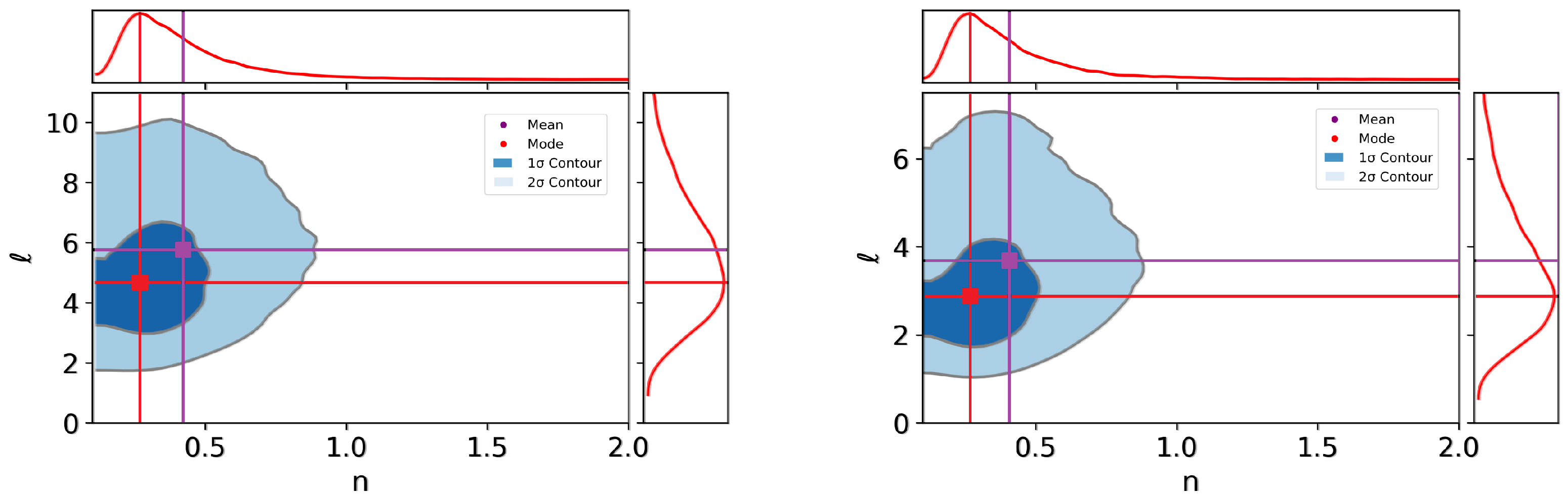
Left: The 1 and 2 confidence contours for the hyperparameters of the Matérn 3/2 kernel (9). Right: The 1 and 2 confidence contours for the hyperparameters of the Matérn 5/2 kernel (10). The posteriors that appear on the top and right sides show the marginal distributions for each hyperparameter. The purple and red color dots show the region of the parameter space where the mean (purple) and mode (red) of each hyperparameter intersects.
Figure 1.
Left: The 1 and 2 confidence contours for the hyperparameters of the Matérn 3/2 kernel (9). Right: The 1 and 2 confidence contours for the hyperparameters of the Matérn 5/2 kernel (10). The posteriors that appear on the top and right sides show the marginal distributions for each hyperparameter. The purple and red color dots show the region of the parameter space where the mean (purple) and mode (red) of each hyperparameter intersects.

Figure 2.
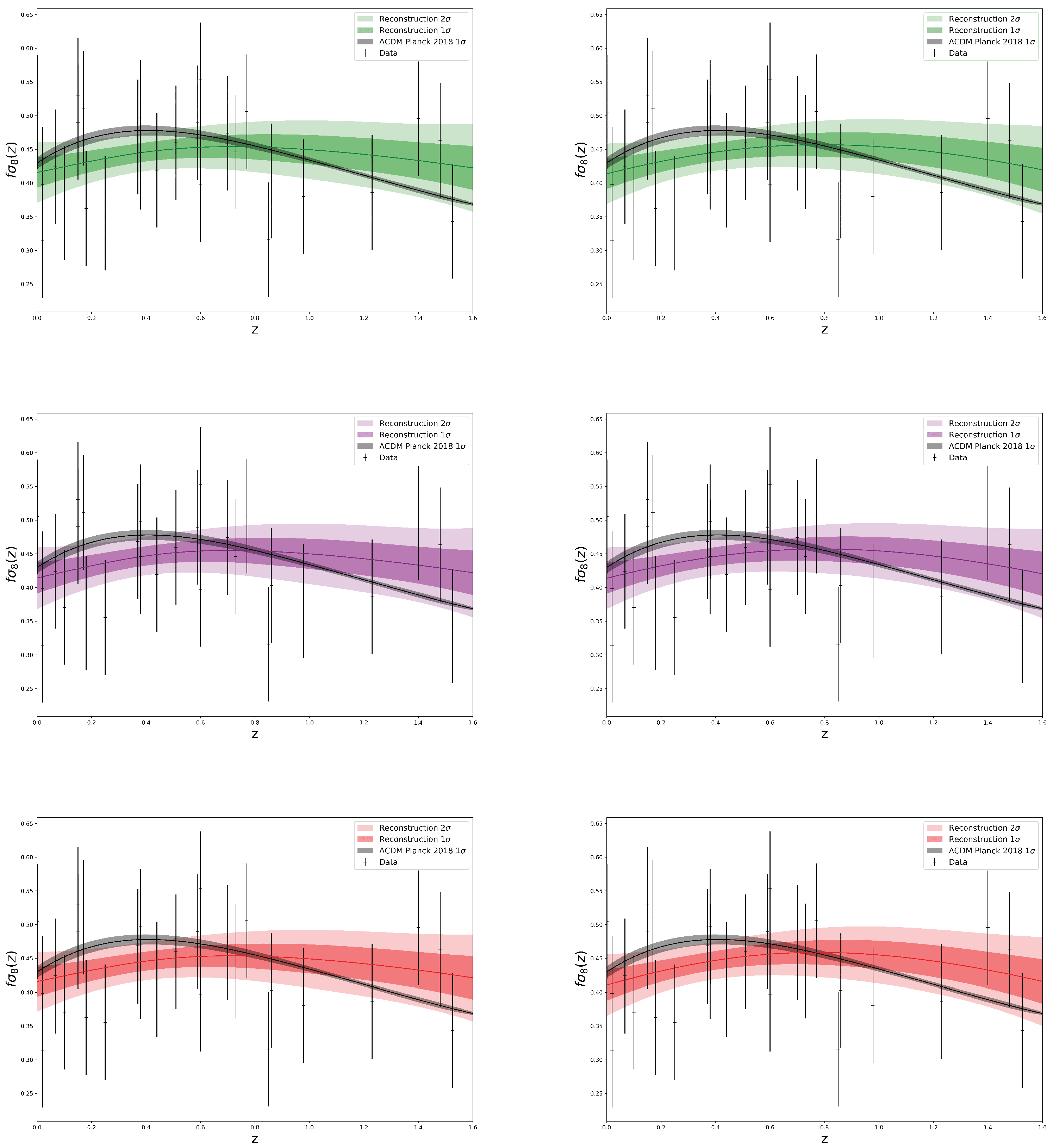
Left: Reconstructions of with the Matérn 3/2 kernel (9). Right: Reconstructions of with the Matérn 5/2 kernel (9). Top: Reconstructions obtained using the maximum likelihood method (green color). Middle: Reconstructions obtained using the mean value of the hyperparameters (purple color). Bottom: Reconstructions obtained using the mode of the hyperparameters (red color). The data are denoted by the black points. In gray we show the prediction for given a fitted CDM with CMB Planck 2018 values [34]. Confidence contours of each reconstruction are shown at the 1 and 2 level.
Figure 2.
Left: Reconstructions of with the Matérn 3/2 kernel (9). Right: Reconstructions of with the Matérn 5/2 kernel (9). Top: Reconstructions obtained using the maximum likelihood method (green color). Middle: Reconstructions obtained using the mean value of the hyperparameters (purple color). Bottom: Reconstructions obtained using the mode of the hyperparameters (red color). The data are denoted by the black points. In gray we show the prediction for given a fitted CDM with CMB Planck 2018 values [34]. Confidence contours of each reconstruction are shown at the 1 and 2 level.


Table 1.
Hyperparameters statistics summary for the Matérn 3/2 kernel (9). The first column indicates the kernel hyperparameters. The second column denotes the value of the maximum likelihood estimation (MLS) for the hyperparameters. The third column shows the mean value of the posterior distribution for each hyperparameter obtained using a MCMC. The fourth column shows the standard deviation. The fifth column indicates the mode.
| Parameter | MLS | Mean Value | Standard Deviation | Mode |
|---|---|---|---|---|
| l | 5.36 | 5.73 | 2.25 | 4.50 |
| 0.33 | 0.42 | 0.24 | 0.26 |
Table 2.
Hyperparameters statistics summary for the Matérn 5/2 kernel (10). The meaning of the columns is the same as in Table 1.
| Parameter | MLS | Mean Value | Standard Deviation | Mode |
|---|---|---|---|---|
| l | 3.33 | 3.71 | 1.70 | 2.80 |
| 0.32 | 0.41 | 0.26 | 0.27 |
Table 3.
Comparison between the different methods analyzed in this work and CDM. The first column shows the method used to estimate the value of the hyperparameters of the Matérn 3/2 kernel. The second column shows the redshift where Equation (13) reaches its maximum; the third column shows the value of reached at that redshift and the fourth column shows the result of integrating in the redshift range where the reconstructions were performed.
| Method | Redshift of Maximum Difference | Maximum Difference | Total Difference |
|---|---|---|---|
| Mean | 0.30 | 2.09 | 1.95 |
| Mode | 0.31 | 2.15 | 2.00 |
| MLS | 0.31 | 2.13 | 1.99 |
Table 4.
Comparison between the different methods analyzed in this work and CDM. The descriptions of the columns are the same as the ones reported in Table 3 but for the Matérn 5/2 kernel.
Table 4.
Comparison between the different methods analyzed in this work and CDM. The descriptions of the columns are the same as the ones reported in Table 3 but for the Matérn 5/2 kernel.
| Method | Redshift of Maximum Difference | Maximum Difference | Total Difference |
|---|---|---|---|
| Mean | 0.3 | 2.18 | 2.12 |
| Mode | 0.3 | 2.17 | 2.06 |
| MLS | 0.3 | 2.19 | 2.12 |
Table 5.
-statistics over the number of degrees of freedom for CDM and the different reconstructions obtained using the kernel Matérn 3/2.
Table 5.
-statistics over the number of degrees of freedom for CDM and the different reconstructions obtained using the kernel Matérn 3/2.
| Method | |
|---|---|
| CDM | 0.85 |
| Mean | 0.77 |
| Mode | 0.78 |
| MLS | 0.77 |
Table 6.
-statistics over the number of degrees of freedom () for the different reconstructions obtained using the kernel Matérn 5/2.
Table 6.
-statistics over the number of degrees of freedom () for the different reconstructions obtained using the kernel Matérn 5/2.
| Method | |
|---|---|
| Mean | 0.78 |
| Mode | 0.77 |
| MLS | 0.78 |
Publisher’s Note: MDPI stays neutral with regard to jurisdictional claims in published maps and institutional affiliations. |
© 2022 by the authors. Licensee MDPI, Basel, Switzerland. This article is an open access article distributed under the terms and conditions of the Creative Commons Attribution (CC BY) license (https://creativecommons.org/licenses/by/4.0/).
Share and Cite
MDPI and ACS Style
Reyes, M.; Escamilla-Rivera, C. On the Degeneracy between fσ8 Tension and Its Gaussian Process Forecasting. Universe 2022, 8, 394. https://doi.org/10.3390/universe8080394
AMA Style
Reyes M, Escamilla-Rivera C. On the Degeneracy between fσ8 Tension and Its Gaussian Process Forecasting. Universe. 2022; 8(8):394. https://doi.org/10.3390/universe8080394
Chicago/Turabian StyleReyes, Mauricio, and Celia Escamilla-Rivera. 2022. "On the Degeneracy between fσ8 Tension and Its Gaussian Process Forecasting" Universe 8, no. 8: 394. https://doi.org/10.3390/universe8080394
Note that from the first issue of 2016, this journal uses article numbers instead of page numbers. See further details here.