

Discrete Event Systems Theory for Fast Stochastic Simulation via Tree Expansion
1
Department of Electrical and Computer Engineering, University of Arizona, Tucson, AZ 85721, USA
2
RTSync Corp., Chandler, AZ 85226, USA
Systems 2024, 12(3), 80; https://doi.org/10.3390/systems12030080
Submission received: 17 January 2024
/
Revised: 22 February 2024
/
Accepted: 27 February 2024
/
Published: 2 March 2024
(This article belongs to the Special Issue Theoretical Issues on Systems Science)
Abstract
:Paratemporal methods based on tree expansion have proven to be effective in efficiently generating the trajectories of stochastic systems. However, combinatorial explosion of branching arising from multiple choice points presents a major hurdle that must be overcome to implement such techniques. In this paper, we tackle this scalability problem by developing a systems theory-based framework covering both conventional and proposed tree expansion algorithms for speeding up discrete event system stochastic simulations while preserving the desired accuracy. An example is discussed to illustrate the tree expansion framework in which a discrete event system specification (DEVS) Markov stochastic model takes the form of a tree isomorphic to a free monoid over the branching alphabet. We derive the computation times for baseline, non-merging, and merging tree expansion algorithms to compute the distribution of output values at any given depth. The results show the remarkable reduction from exponential to polynomial dependence on depth effectuated by node merging. We relate these results to the similarly reduced computation time of binomial coefficients underlying Pascal’s triangle. Finally, we discuss the application of tree expansion to estimating temporal distributions in stochastic simulations involving serial and parallel compositions with potential real-world use cases.
1. Introduction
Stochastic simulations require large amounts of time to generate enough trajectories to attain statistical significance and estimate desired performance indices with satisfactory accuracy [1,2,3]. Complex problems such as climate change mitigation, network design, and command and control decision support require search spaces with deep uncertainty arising from inadequate or incomplete information about the system and the outcomes of interest [4,5,6,7,8,9,10]. Furthermore, simulation models for system engineering analyses present challenges to today’s computational technologies. First, questions addressed at the Systems of Systems (SoS) level require large detailed models to provide sufficient representation of relevant system-to-system interactions of stochastic nature. Second, they also require multiple executions with multiple random seed state initiations to cover the wide range of configurations necessary to obtain statistically significant measurement of performance outcome distributions.
Surrogate models, i.e., simplified models which drastically reduce computation while providing useful guidance, have successfully helped find global optima of computationally expensive optimization problems for real-world applications [11,12,13,14,15,16]. The methods using such models are often referred to as multifidelity/multilevel/variable-fidelity optimization. We note that the term fidelity is often employed to refer to ambiguous combinations of resolution and accuracy [17,18]. A generic framework was defined [19] in which models of different accuracy and computation costs are selected algorithmically to reduce the overall computational cost while preserving the accuracy of the simulation analysis. While such frameworks exist, they do not by themselves provide the surrogate models or more generally methods for speeding up the simulation of stochastic systems to support more timely systems analysis and optimization [20,21,22,23,24,25].
The parallel execution of simulations offers another avenue for the speedup of complex simulations. Unfortunately, exploitation of the parallelization of simulation models for generic system engineering analyses presents challenges to today’s computational technologies [26,27]. Although technological advances at the hardware level will enable more and faster processors to handle such simulations, with cloud services adding access to additional resources, such computational support is destined to reach its limit. Therefore, the imperative remains to formulate parallelization in more model-centric ways. Paratemporal and cloning simulation techniques have been introduced that increase opportunities for parallelism [28,29].They also exploit abstractions that recognize the effect of random draws on system evolution as constituting choice points with opportunities for reuse [30]. However, scalability, the ability to overcome the combinatorial explosion of branching arising from multiple choice points, presents a major hurdle that must be overcome to implement such techniques.
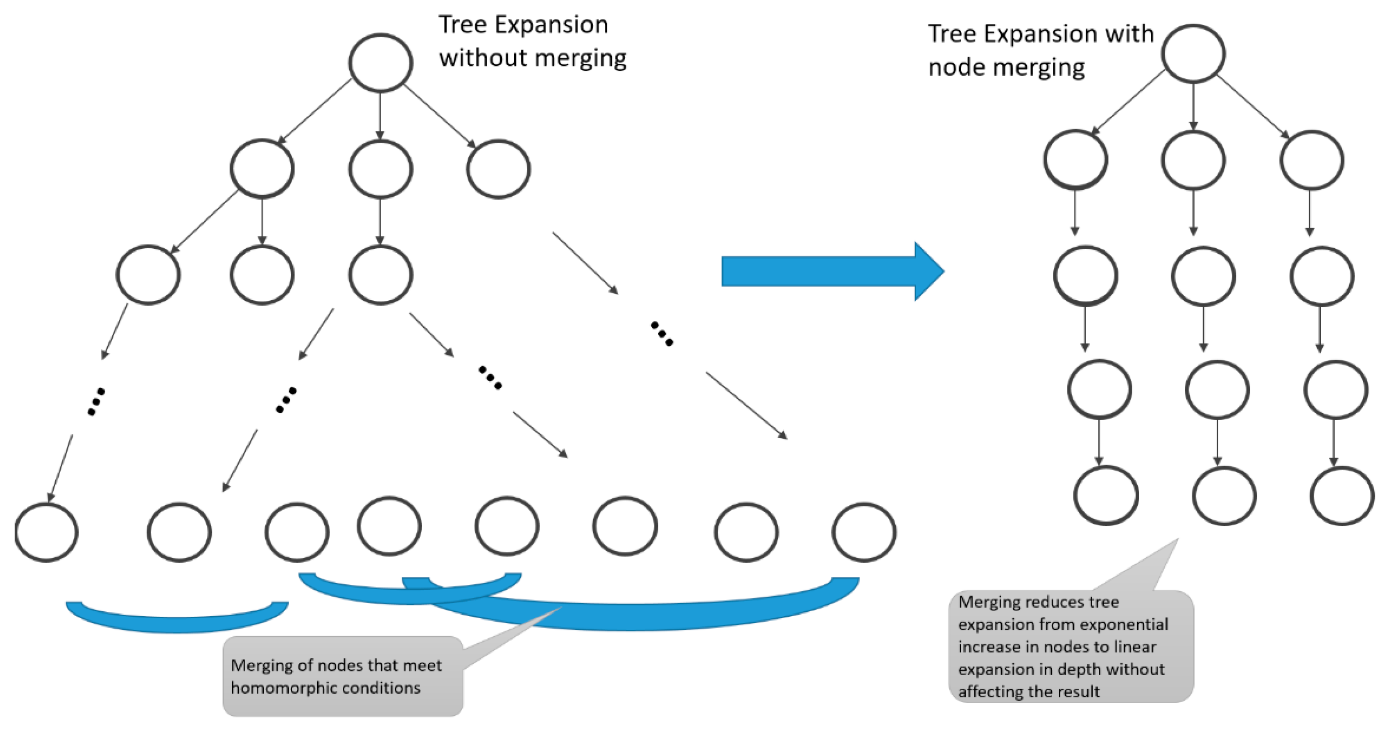
Nutaro et al. [31] examined the use of tree expansion methods in lieu of the conventional sampling of outcomes when working with the uncertainty inherent in stochastic simulations. Conventional techniques simulate a large number of randomly sampled trajectories from start to finish in one-at-a-time fashion. As illustrated on the left side of Figure 1, such trajectories can be viewed as paths from an initial state of the stochastic system (the root of the tree) to one of the terminal states, leaves of the tree, in a manner consistent with random sampling. The advantage of tree construction is that states of the model that have been reached at any point—nodes of the tree—can be cloned for reuse, thus avoiding duplication. Branches in the tree from a state correspond to draws of the random variable whose values determine the subsequent course of the model from that state.
In particular, tree expansion with breadth-first traversal can significantly speed up the computation required to generate the same sampling outcomes as the one-at-a-time technique [31]. However, the speedup is limited by the exponential growth of the tree with increasing depth. Zeigler et al. [32] introduced merging of states based on homomorphism concepts to mitigate against such growth. As illustrated on the right-hand side of Figure 1, they showed that such merging can reduce tree growth from exponential to polynomial in depth, thus significantly speeding up computation over that possible with cloning alone.
Parallelizations of such simulations have been developed in which simulations are run until a stochastic decision point is reached. At this point, the current simulation states and probabilities of branching are saved. Simulations are then spawned for possible branchings until successive downstream branching points are reached, and the process is repeated until a satisfactory level of confidence in outcome distribution has been attained. Besides being efficient in exploration, this “paratemporal” approach is extremely parallelizable for great efficiency in execution on multiple processors.
However, although paratemporal simulations with a small number of branchings and state saves have been demonstrated to be effective, simple implementations of such solutions do not scale as the number of branches increases rapidly for large SoS of current interest.
In this paper, we tackle the scalability problem by first developing a formal framework covering conventional and proposed tree expansion algorithms for speeding up stochastic simulations while preserving the desired accuracy. Based on the theory of modeling and simulation, we review the definition of a discrete event stochastic model as an instance of a timed non-deterministic model. Then, we show how a reduced deterministic model with random inputs can be derived from such a stochastic model that represents the results of cloning state and transition information at branching points. The reduced model is shown to be a homomorphic image of the original based on a correspondence restricted to non-deterministic states and multi-step deterministic sequences mapped into corresponding single-step sequences. An example is discussed to illustrate the tree expansion framework in which the stochastic model takes the form of a binary tree isomorphic to the free monoid, {0,1}*. At each node, branching occurs with equal probability to nodes at the next level. A computation time of 1 unit is taken to transition from a node to its successor. The output at a state is the number of 1′s in its label. We derive the computation times for baseline, non-merging, and merging tree expansion algorithms to compute the distribution of output values at any given depth. The results show the remarkable reduction from exponential to polynomial dependence on depth effectuated by node merging. We relate these results to the reduced computation of binomial coefficients underlying Pascal’s triangle and discuss the application of tree expansion to estimating temporal distributions in stochastic simulations involving serial and parallel compositions. Finally, we mention use cases estimating times to completion for complex processes and potential real-world applications.
2. Formal Framework for Tree Expansion for Stochastic Simulation
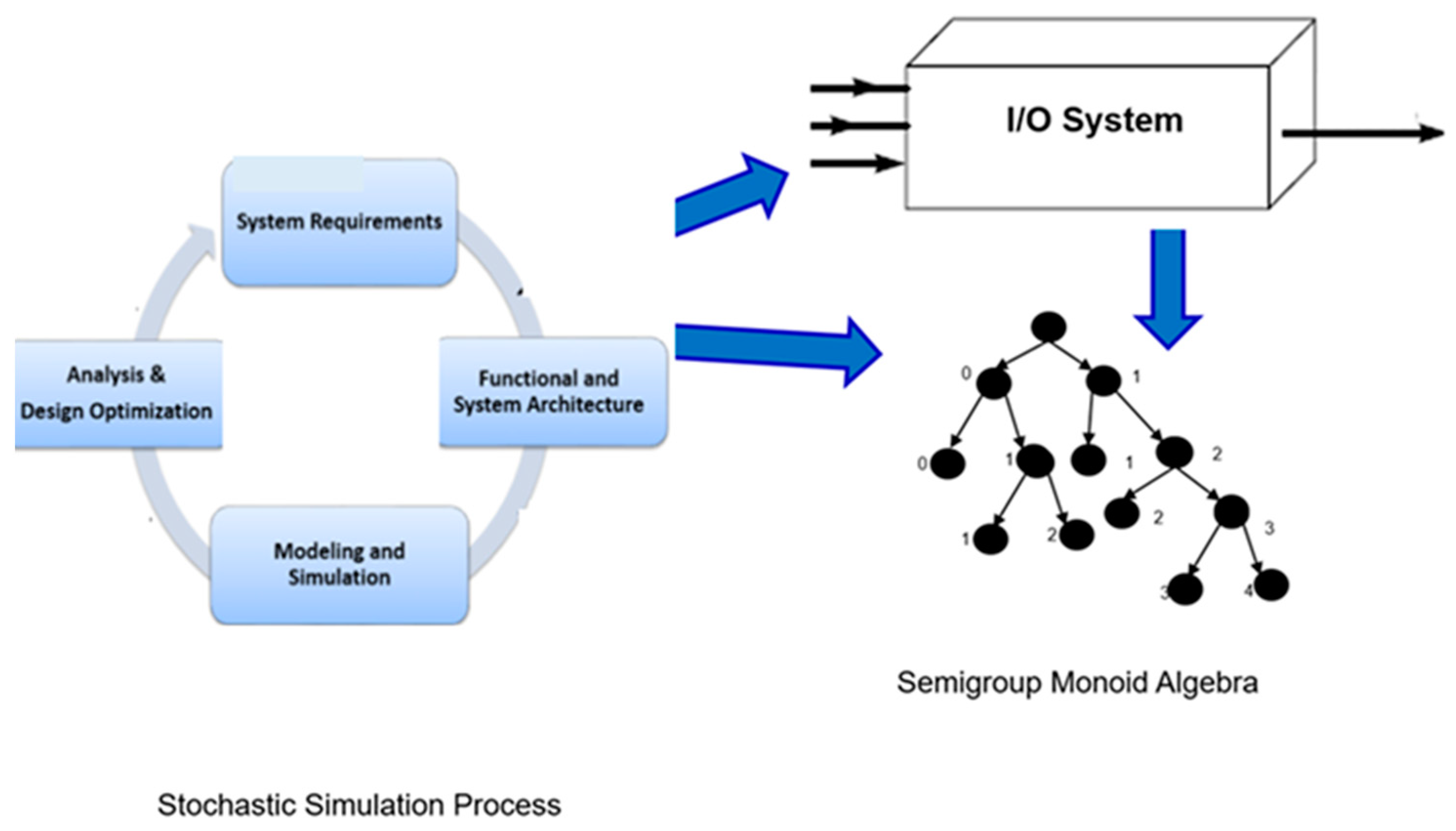
We employ the theory of modeling and simulation [33], based on systems theory [34], to develop a formal framework based on Discrete Event Systems Specification (DEVS) for framing the representations needed for paratemporal simulations. As in Figure 2, to capture the effect of cloning on the source stochastic simulation, we derive other representations including concepts of non-deterministic models and semigroup monoid algebras.
2.1. Definitions
We review some definitions to proceed.
Definition 1.
A timed non-deterministic model is defined by M = <S, δ, ta>, where δ ⊆ S × S is the non-deterministic transition relation and ta: δ→R∞0 is the time advance function.
We say that M is as follows:
- Not defined at a state, if there is no transition pair with the state as its left member;
- Non-deterministic at a state, if the state is a left member of two transition pairs;
- Deterministic at a state when there is exactly one outbound transition (a left member of exactly one transition pair).
Remark: Formulating a transition system in relational form as in Definition 1 allows us to include both stochastic and deterministic discrete event systems within a common framework as follows:
Figure 2.
DEVS-based framework for framing the representations needed for paratemporal simulations.

A stochastic model is a timed non-deterministic model defined in all of its states.
A deterministic model is a timed non-deterministic model (Figure 3) deterministic in all its states.
Clearly, deterministic models are a subset of stochastic models.
In application to paratemporal simulation, a non-deterministic state is known as a random draw state. We make this identification in a later section after introducing DEVS Markov models.
Definition 2.
A state trajectory connecting a pair of states, s and s’, is a sequence s1, s2,…, sn which starts with s and ends with s’ and satisfies the transition relation, i.e., where s1 = s, sn = s’ and δ(si,si+1) for i = 1,…,n−1.
Definition 3.
A deterministic state trajectory is a state trajectory containing only deterministic states. The time to traverse a deterministic state trajectory is the sum of the transition times associated with the successive pairs of states in its sequence.
We can remove deterministic states from a stochastic model and replace multi-step deterministic trajectories with single-step trajectories to represent the effect of cloning simulations. Given a stochastic model, M = <S, δ, ta>, we define a reduced version that contracts deterministic sequences into single-step transitions:
Definition 4.
The clone-reduced version of stochastic model M = <S, δ, ta> is
where
M’ = <S’, δ’, ta’>
- S’⊆ S is the subset of non-deterministic states of M
- δ’⊆ S’ × S’ = {(s,s’)| if there is a deterministic state trajectory connecting s and s’}
- and ta’: δ’→R0∞
where
We can prove the following.
2.2. Assertion 1
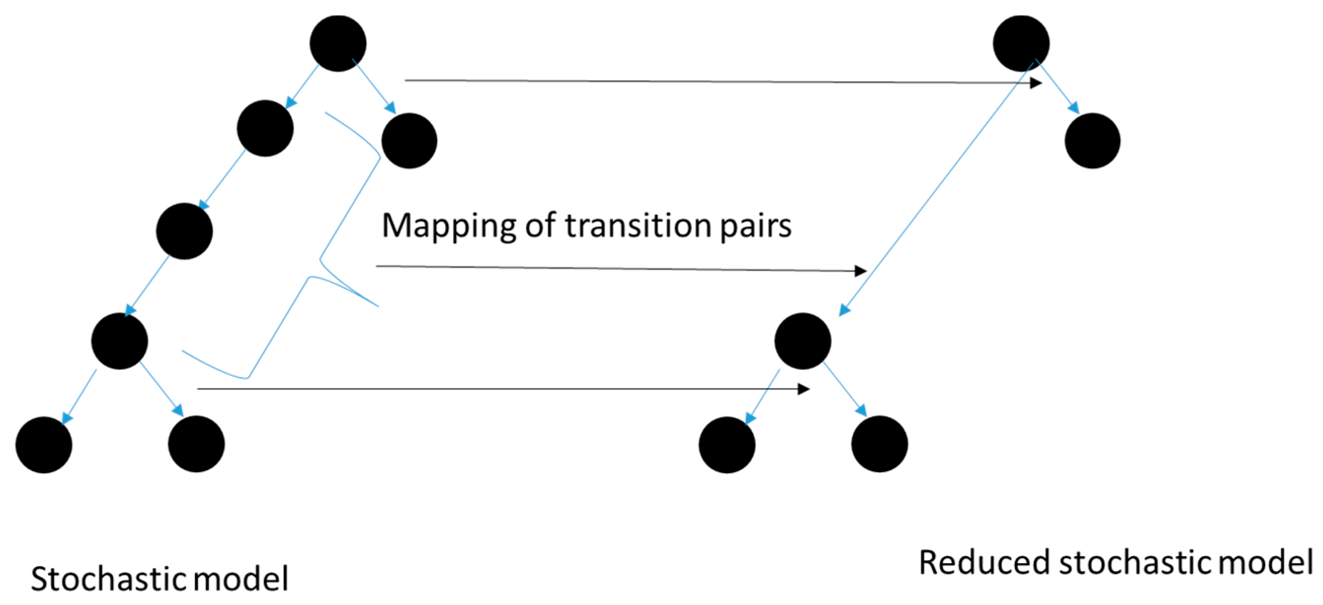
The reduced model is a homomorphic image of the original based on a correspondence restricted to non-deterministic states and multi-step deterministic sequences mapped into corresponding single-step sequences (Figure 4).
We note that the transversal time from any non-deterministic state to any other is preserved in the reduced version. However, the advantage of constructing this representation is that the computation (in simulation) of a multi-step sequence can be replaced by a look up of a table (cloning) when the branching is encountered subsequently.
Definition 5.
MST= <Y,S, Gint, Pint, λ, ta>
where Y, S, λ, and ta have the usual definitions [35].
Here Gint: S→2S is a function that assigns a collection of sets Gint (s) ⊆ 2S to every state s.
The probability that the internal transition carries a state s to a set G ∈ Gint (s) is given by a function Pint (s,G).
For S finite, we let
where Pr(s, s’) is the probability of transitioning from s to s’.
As defined in [33], the key to formalizing a semi-Markov model in DEVS is the definition of two structures. One corresponds to the usual matrix of probabilities for state transitions. The other assigns to each transition pair a probability density distribution over time. The choice of the next phase in the DEVS is made first by sampling the first matrix. Then, the transition from the current phase to the just-selected next phase is given a time of transition by sampling the distribution associated with that transition. More formally, this is formulated by the following:
Definition 6.
A pair of structures, probability transition structure, PTS = <S, Pr>, and time transition structure, TTS = <S, τ>, gives rise to an input-free DEVS Markov model [33]. MDEVS = <Y,SDEVS, δint, λ, ta>, where SDEV S = S × [0, 1]S × [0, 1]S, with typical element (s, γ1,γ2) with γi: S → [0, 1], i = 1, 2, where,
- δint: SDEV S→SDEV S is given by
- δint (s, γ1,γ2) = s’ = (SelectPhase Gint (s, γ1), γ1′, γ2′)
- and ta: SDEV S→R+0,∞ is given by
- ta(s,γ1,γ2) = SelectSigma TT S (s, s’,γ2)
- and γi’ = Γ(γi), i = 1, 2.
The input-free DEVS Markov model is introduced as a concrete implementation for non-deterministic models. On the one hand, such models are constructible in computational form in such environments as MS4 Me [36]. On the other hand, we can explicitly define how such models give rise to non-deterministic models as in the following:
2.3. Assertion 2
An input-free DEVS Markov model MDEV S = <Y,SDEV S, δint, λ, ta> specifies a non-deterministic model M = <S’, δ’, ta’>, where S’= SDEVS, δ’ ⊆ S’ × S’ is given by (s1,s2) is in δ’ if, and only if, there exists γ1 in [0, 1],γ2 in [0, 1], such that, δint (s1, γ1,γ2) = s2, and ta’: δ→R∞0 is given by ta’(s1,γ1,γ2) for the same pair (γ1,γ2) that placed (s1,s2) in δ’.
Essentially, this assertion shows how a transition from state s1 to s2 is possible if there is a random selection of s2 from the set of possible next states of s1 (as determined by the seed γ1), and the time for such a transition is given by a sampling from the distribution for traversal times determined by the seed γ2.
3. Illustrative Example
To create the models needed to illustrate the framework of Figure 1, consider a binary tree of depth 3 with root labelled by the empty string and each node labelled by a string of 0’s and 1’s corresponding to the path to it from the root. At each node, a choice is made to select the successor to which to transition with equal probability. A computation time of 1 unit is taken to transition from a node to its successor. The output at a state is the number of 1’s in its label. We write the formal representation as a DEVS Markov model as follows:
MDEV S = <Y, SDEV S, δint, λ, ta>
Y = {0, 1, 2, 3}
S = {0, 1, 00, 01, 10, 11, 000, 001,…111} (nodes in a binary tree of depth 3 labelled by strings corresponding to the path accessing them). SDEV S is the set of pairs of the form (s, γ) where s is a member of S (a node) and γ is a state of an ideal random number generator, such that Γ (γ) is the next state of the random generator (for simplicity, the time advance will be constant so an additional random variable is not needed).
Gint (s) = {s0,s1}, the subset of nodes that are immediate successors of node s in the binary tree and
where SelectPhase Gint (s, γ) uses the random number state γ to select the successor node from Gint (s) with equal probability.
And λ(s) is the number of 1’s in the label of s.
s’ = δint (s, γ) = (SelectPhase Gint (s, γ), Γ(γ))
ta(s,γ) = 1
The desired outcome of the simulation is the average of the values of the nodes.
To illustrate the applicability of homomorphism and the minimal realization concept, we will show how it provides insight into the merging of states for tree expansion.
We will compare the following three algorithms:
- The baseline algorithm generates all trajectories one at a time, accumulates the number of 1’s for each, and averages the results.
- The tree expansion algorithm generates all nodes in breadth-first traversal without repetition, obtaining the same information and performing the same average.
- The node merging algorithm based on the minimal realization modifies tree expansion by maintaining only the representatives of equivalent classes as successive levels are generated while maintaining the size of the classes as they are developed. The values of the classes are summed weighted by the respective sizes to obtain the desired average.
The node merging Algorithm 1 is sketched in the following:
| Algorithm 1. Node merging tree expansion algorithm. |
| A node n contains data {s, num) where s is a string in {0,1}* and num is the number of nodes equivalentTo n. The root node = (λ,1) //λ is the empty string is the empty string Initiation: Current node = root node; newLeaves = {}, oldLeaves = {(λ,1)} Termination: depth = D Output: For each i = 1,2,…,D the number of strings having number of ones equal to i. Depth = 0 Recursive step: While (depth < D) For each node, n = (s, num) in leaves{ For each branch, b in {0, 1}{ Create child, c = {sb, num) // extend parent’s string and inherit parent’s number of represented equivalents If c is Equivalent To some node, m = {t, num’) in newLeaves, Then set m = {t, num’+num) Else add c to newLeaves. } depth = depth+1 oldLeaves = newLeaves, newLeaves = {} } n = (s, num) isEquivalentTo m = {t, num’) if, and only if, s and t have the same number of ones //Note that only the leaves at each level (including at the final depth) are kept as the expansion advances as required by the required output. |
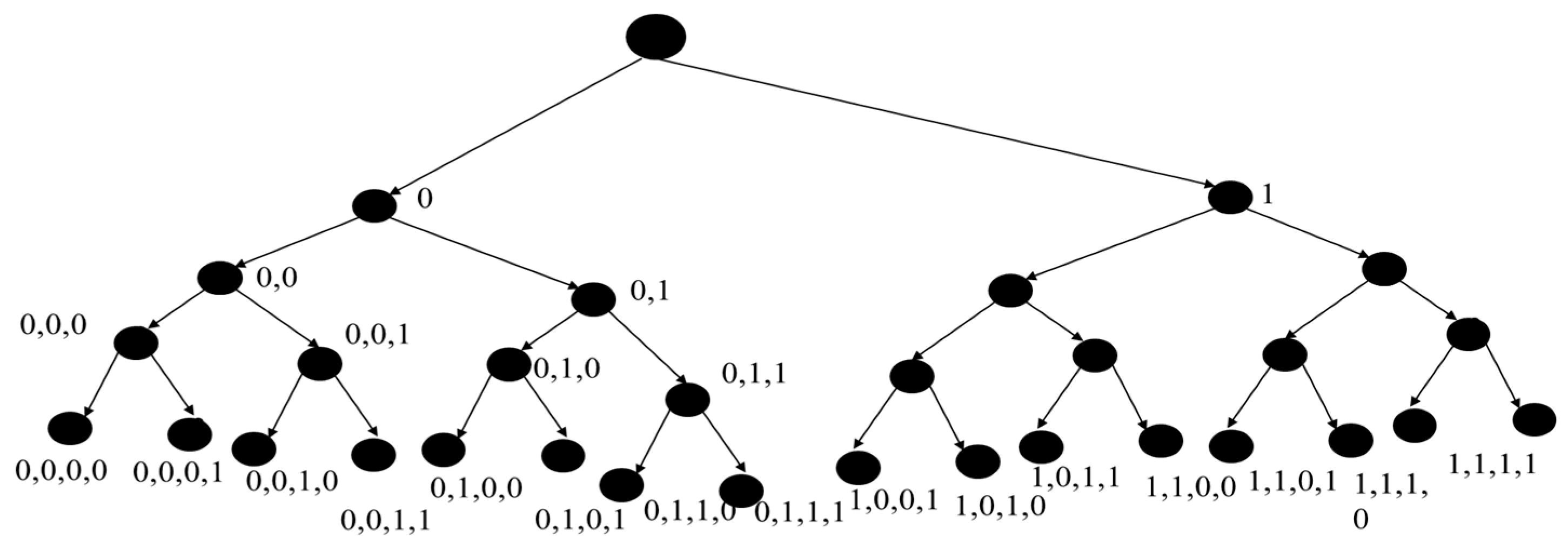
To analyze this example, we will start with the semigroup monoid system (as in the Appendix A) unfolded to the depth = 4, as shown in Figure 5. The leaves of the tree are labelled with the final states listed above, and traversing the tree from root to leaves reveals 16 branching routes. We will proceed to obtain various computation times generalized to the case of a tree of arbitrary depth n, as presented in Table 1. The computation time for the baseline algorithm is computed as the number of branching routes (2n) times the depth (n) taking unit computation time per step. The smallest number of computations when reusing earlier nodes is to expand the tree starting at the root and proceeding to expand new leaves successively at each level in breadth-first traversal. This requires 2(2n−1) computations, as shown in the table. Therefore, the reduction in computation time is n2n/2(2n−1) which is of order O(n).
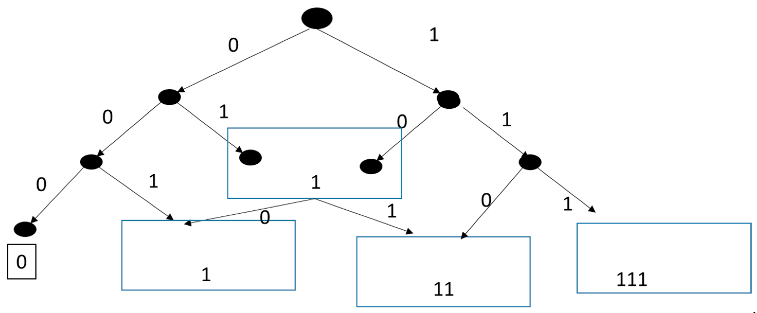
The minimal realization of this model, shown in Figure 6 to depth = 3, recognizes that all nodes labeled (x1,x2,x3) with the same sum (x1 + x2 + x3) can be grouped into the same congruence class. The justification of congruence is easy to see in this case: the 0 input keeps such an element in the same class, while the 1 input transitions it to the class having a sum increased by 1. With the merging of nodes, the tree expands in a manner emulating Pascal’s triangle for computing binomial coefficients [37]. At any depth n, there are a total of 2n subsets of sizes ranging from 0 to n with cardinalities given by the binomial coefficients. For example, at depth 3, there are 1,3,3,1 subsets of sizes 0,1,2,3, respectively. With the size of a subset representing the number of 1’s in the same equivalence class, we see that the average number of 1’s will equal n/2, as expected. Importantly, the number of nodes, and hence the computation time, grows only as the square of n rather than exponentially, as shown in Table 1. The computation time is now O(n2) (square) in the depth of the tree, and the reduction is of exponential order—which would be exceedingly impressive to achieve in real-world application!
4. Empirical Confirmation of Theory Predictions
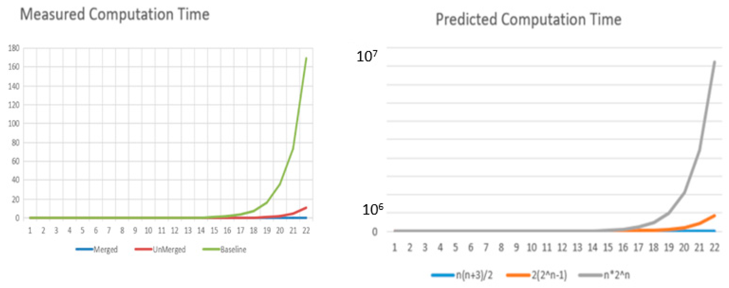
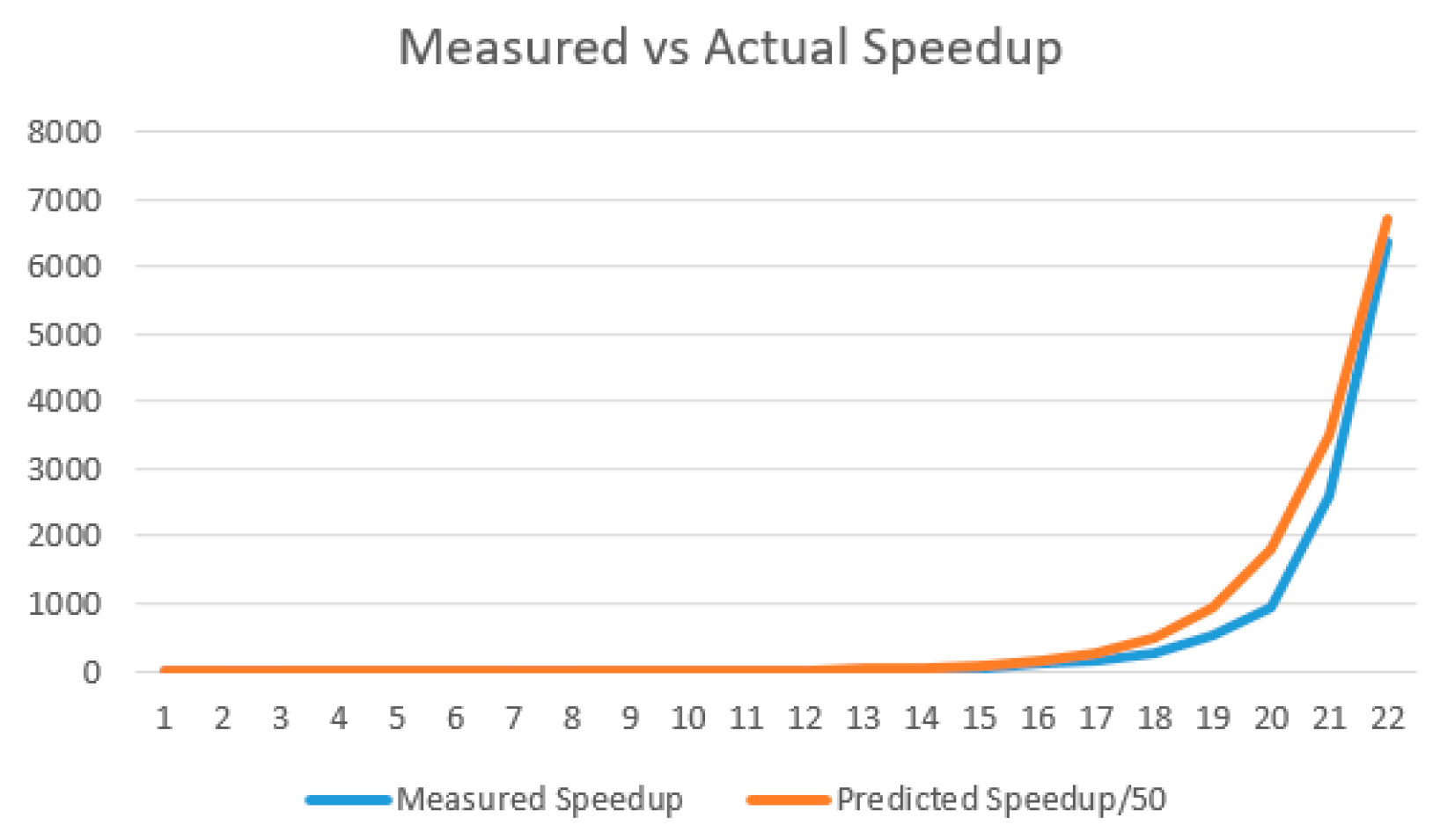
To test the theory and its implementation, the illustrative example was implemented in Java and executed to compare computation times with those predicted from Table 1. Figure 7 shows that the relative computation times of the merged, unmerged, and baseline algorithms fall in the order of that predicted in Table 1. However, Figure 8 shows that the actual speedup realized by merging relative to the baseline is approximately 50 times less than predicted. Nevertheless, the speedup achieved at depth 22 of approximately 7000 is still highly significant. Note: the baseline algorithm exceeds the memory available at depth 23 due to the exponential node growth. Trees up to depth 1000 with 10 replications for each were tested to obtain the timing results, and all yielded the correct outcome distribution.
5. Tree Expansion with Merging Applied to Serial and Parallel Compositions
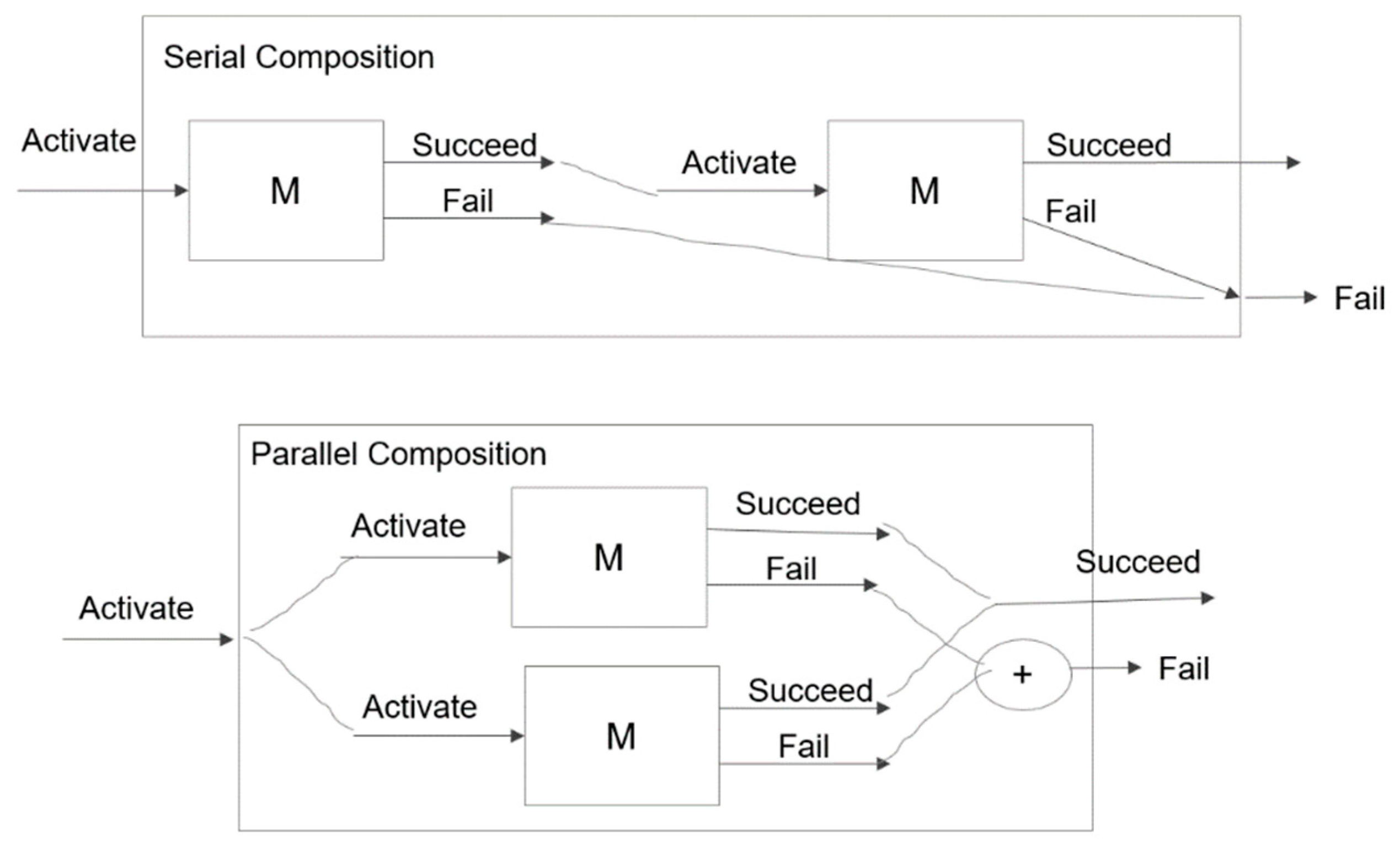
Serial and Parallel compositions of simple DEVS Markov models illustrate how merging in tree expansion can work in a large class of stochastic systems to greatly control node generation and computation time. To succeed, a serial composition entails the success of each of its components; likewise, it fails if any one of its components fails [38]. In contrast, the success of a parallel composition requires that only one of its components succeeds, while its failure entails the failure of all the components.
The component models in the compositions are of the form of a DEVS Markov model (not including input and output), as shown in Figure 9 and Figure 10.
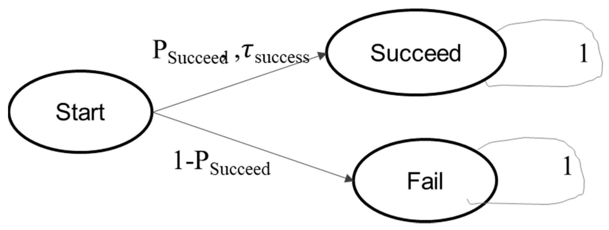
The transition structure of the model is specified by two parameters, PSucceed, the probability of success, and succeed, the probability distribution for the time required to achieve success. These populate the values of the probability and the time transition structures needed for the definition of the model, which is given as follows:
SDEV S is the set of triples of the form (s, γ,) where s is a member of S (a node) and γ, are states of ideal random number generators for selecting between the transitions from Start to Succeed or Fail and for selecting the time distribution for the transition to Succeed, if selected. The time for the transition to Fail is not of interest here so no random seed is associated with it.
Gint (Start) = {Succeed,Fail} the subset of nodes that are immediate successors of node Start, and s’= δint (Start, γ,) = (SelectPhase Gint (Start, γ), Γ (γ),), where the latter uses the random number seed γ to select Succeed with probability PSucceed, and Fail with probability 1 − PSucceed. ta(Succeed, γ,) = (SelectSigma Gint (Start, γ, )) which selects the time required to succeed from the given distribution, succeed, and λ is the time selected for the time advance.
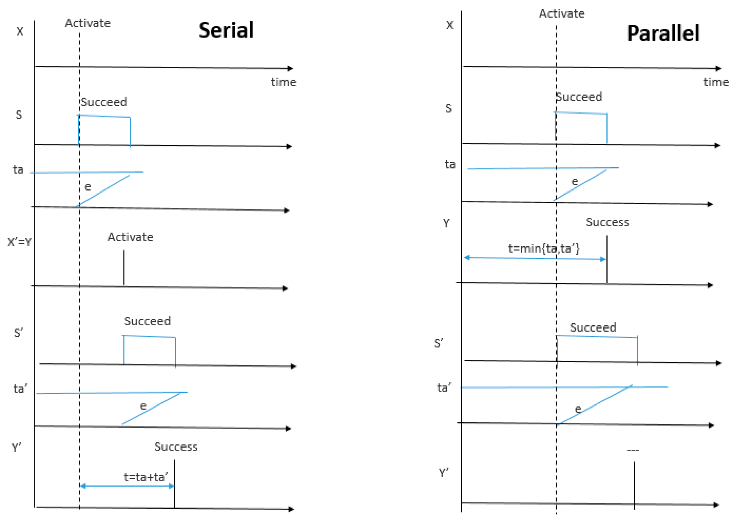
Serial and parallel compositions in Figure 9 and Figure 10 are defined using the standard DEVS coupled model specifications [33]. As illustrated in Figure 11, the temporal behaviors of the compositions are directly derived from those of the components and the coupling specified by the respective composition.
In the serial composition, the Activate input is shown setting the first (top) model, M into state Succeed with an output after time ta. The latter is determined by the random sampling process just described and shown as a threshold value for the elapsed time, e to achieve. This output, Y is coupled to the input of the second component (bottom) model, M’ and causes it to output a final Success after ta’ for a total response time of ta + ta’.
In the case of the parallel composition, the Activate input starts both models simulta-neously and results in a Success output from the quickest model at time min{ta,ta’}.
These paired configurations are easily generalized to finite numbers of components where, for the serial composition, components are placed in a sequence with the Success output port of one connected to the Activate input port of the next, and for the parallel composition, all components receive activation simultaneously with all output Success ports coupled to the overall output Success port. The desired outcome of the simulations of the compositions is the probability distribution of time needed for success. In the serial case, a sampled value of this outcome is the sum of the time samples from each component since all have to succeed for the whole to succeed. In the parallel case, a sampled outcome is the minimum of the sampled durations of the components since overall success is achieved by the first to succeed. Analytic solutions such as those by Rice [38] are possible given analytic input distributions, but stochastic simulation is needed otherwise.
Computation Time Required for Serial and Parallel Compositions
In application to serial and parallel compositions, the number of components determines the depth of the tree, n. The temporal distribution of each component is assumed to be known and represented by a discrete probability density over an interval divided into G segments, where G is called the number of granules and determines the accuracy of the computed outcome. In the following, we simplify the discussion by considering only the case where the probability of failure is zero.
Tree expansions for the series and parallel compositions in Figure 12 evolve with G branches stemming from each node. For the serial compositions, with the first model at level 1, each of the G branches from the root is labelled by the time advance corresponding to the granule represented by that branch. For each of the nodes generated by such branching, the second model’s response is represented by the branching of G nodes at level 2 labelled by the time advances corresponding to each. Response times, t = ta + ta’, for the composition are accumulated in the nodes terminating the paths labelled by the pairs of branches. In the case of parallel composition, the only difference is that the minimum operation is applied to the pair of time advances to be stored in the node terminating the corresponding path.
Therefore, we see that in both serial and parallel compositions, the unmerged tree expands with Gn nodes at depth n. However, as the tree front expands, applying the merging process to nodes at the same level greatly reduces the number of nodes that must be considered as the depth increases. Merging in the case of serial composition only adds G nodes at each level, thus reducing the growth in nodes to nG. This is so since at each successive level the range of sum ta + ta’ is bounded above by max{ta} + max{ta’}. Thus, after merging, only G new nodes are added to that level. Moreover, at each level, the number of operations is at most nG2 since the nG nodes are combined with the G granules to create the next level. Thus, the incremental computation time is nG2, and the computation time required should grow as O((nG)2), i.e., as the square of depth and number of granules.
Merging in the case of parallel composition does not suffer any tree expansion since the combined range of a minimization is the original range, i.e., range of min{ta,ta’} is bounded above by min{max{ta},max{ta’}}. Thus, by the reasoning above, the number of nodes grows as n*G and the operations grow as nG2. So, the computation time required for depth n should grow as O(nG2), i.e., linearly with the depth and square of granules.
6. Related Work
DEVS has served as a basis for the formalization [38,39] and study of multiresolution constructions underlying multifidelity simulations [40,41,42,43,44,45]. Also, DEVS has been employed as a basis for the simulation of Markov Decision Process (MDP) models employing its modular and hierarchical aspects to improve the explainability of the models with application to optimization processes such as financial, industrial, etc. [46,47,48,49,50,51,52]. Capocchi, Santucci, and Zeigler [53] introduced a DEVS-based framework to construct and aggregate Markov chains using a relaxed form of lumpability to enhance the understanding of complex Markov search spaces. However, the methodology is limited to selecting optimal partitions according to a metric that compares Markov chains based on their respective steady states. The practical application is limited since these are not generally available in problem specification. In contrast, paratemporal and cloning simulation techniques are intended for application to stochastic simulation in general and offer opportunities for parallelism and cloning of state information. However, they have not demonstrated the ability to overcome the combinatorial explosion of branching arising from multiple choice points. The absence of such scalability presents a major hurdle that must be overcome to implement such techniques. Nutaro et al. [31] showed that the speedup of tree expansion methods is limited by the exponential growth of the tree with increasing depth. Zeigler et al. [54] introduced the merging of states based on homomorphism concepts to mitigate against such growth. Here, we demonstrated that homomorphic merging of states can be formally characterized using DEVS Markov modeling and simulation theory to show examples where such merging can achieve a reduction from exponential to polynomial computational effort.
7. Conclusions and Further Work
We have developed a formal framework covering conventional and proposed tree expansion algorithms for speeding up stochastic simulations while preserving the desired accuracy. Based on the theory of modeling and simulation, we showed how a reduced deterministic model with random inputs can be derived from such a stochastic model. This reduced model represents the results of cloning state and transition information at branching points. The reduced model was shown to be a homomorphic image of the original based on a correspondence restricted to non-deterministic states and multi-step deterministic sequences mapped into corresponding single-step sequences. An example was discussed to illustrate the tree expansion framework in which the stochastic model takes the form of a binary tree, allowing us to derive the computation times for baseline, non-merging, and merging tree expansion algorithms to compute the distribution of output values at any given depth. The results show the remarkable reduction from exponential to polynomial dependence on depth effectuated by node merging. We related these results to the reduced computation of binomial coefficients underlying Pascal’s triangle.
Applications of node merging tree expansion algorithms are currently being studied in simulations of space-based threat responses to estimate the probability of successfully identifying, tracking, and targeting hypersonic missiles within tight deadlines [38], as well as to attrition modeling employing stochastic interactions between opposing forces [55,56,57,58,59,60]. In such models, temporal duration outcomes in the form of probabilistic temporal distributions play a major role, and homomorphic merged tree expansion enables much faster computation of outcome distributions when analytic solutions are lacking.
Funding
This research was partially supported by RTSync internal funding and received no ex-ternal funding.
Data Availability Statement
Data sharing not applicable.
Acknowledgments
I would like to thank Sang Won Yoon, and Cole Zanni, Graduate Research Associate at the Watson Institute for Systems Excellence at The State University of New York at Binghamton, NY, and Christian Koertje, Research Assistant at University of Massachusetts, Amherst, MA, for their help in working on the algorithm implementations.
Conflicts of Interest
The author declares no conflicts of interest.
Appendix A
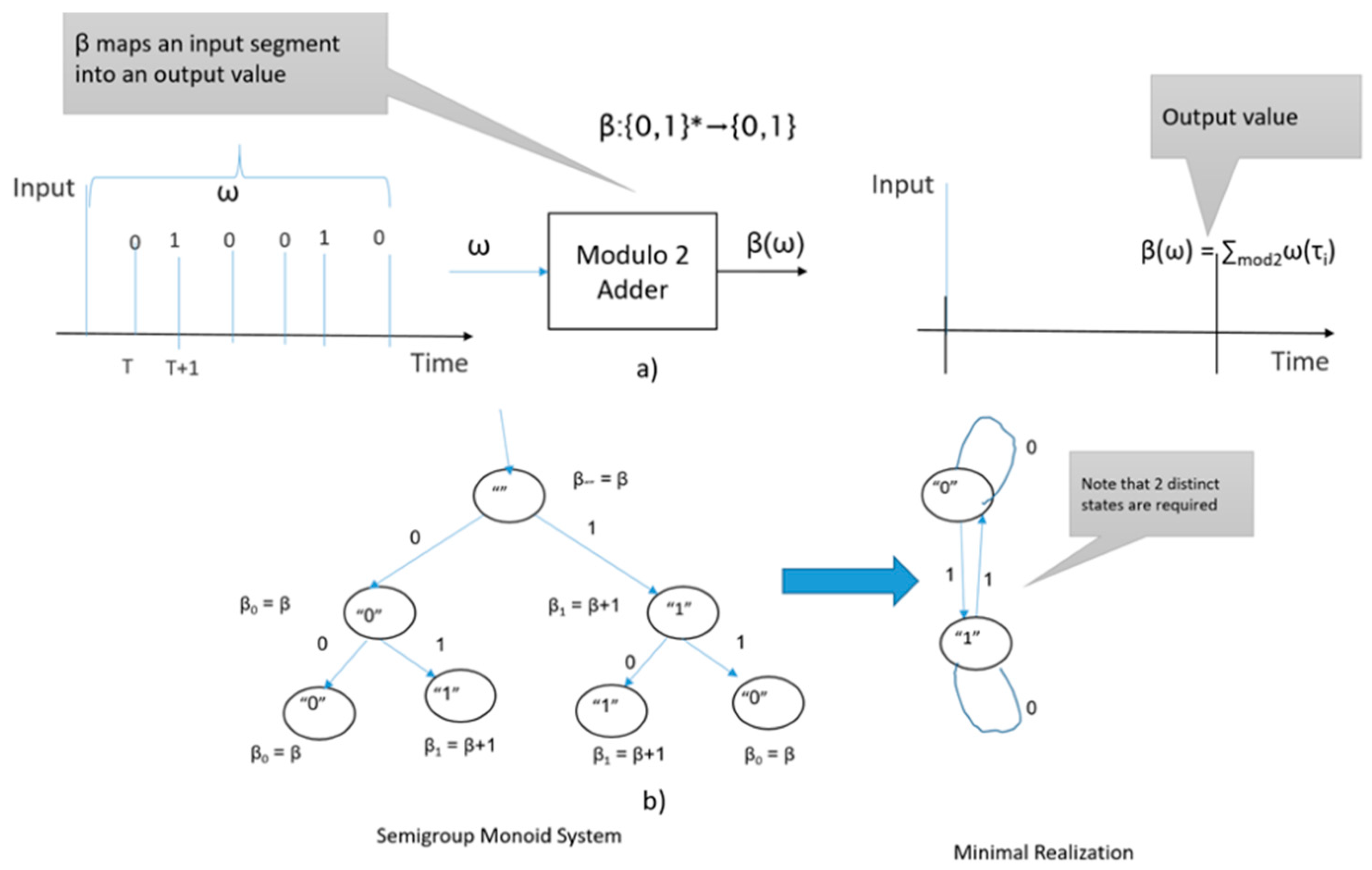
We define the behavior of a system formally as a function mapping input segments to output segments (Figure 6). We seek a DEVS model at the state description level that generates the defined behavior and then try to show it is a minimal realization or attempt to reduce it to one that is minimal.
We briefly review the approach to deriving a minimal realization from an input time function description. Figure A1a shows the behavior of a modulo 2 adder, and the minimal realization is in Figure A1b. The latter has two states corresponding to the two distinct nodes with transitions reflecting and alternating pattern exhibited by the derivatives of the behavior β in the tree. The alternating pattern is manifested by noticing that β0(ω) = β(0ω) and β1(ω) = β(1ω) so that the state “0” transitions to itself under input 0 and transitions to the state “1” under input 1.
Figure A1.
(a) Mapping input segments to output segments, (b) states reduction and minimal realization. Note: {0.1}* denotes the set of all finite strings over {0,1}.
Figure A1.
(a) Mapping input segments to output segments, (b) states reduction and minimal realization. Note: {0.1}* denotes the set of all finite strings over {0,1}.

References
- Müller, J.; Shoemaker, C.A.; Piché, R. SO-MI: A surrogate model algorithm for computationally expensive nonlinear mixed-integer black-box global optimization problems. Comput. Oper. Res. 2013, 40, 1383–1400. [Google Scholar] [CrossRef]
- Zabinsiky, Z.B. Stochastic Adaptive Search Methods: Theory and Implementation. In Handbook of Simulation Optimization; Springer: New York, NY, USA, 2015; pp. 293–318. [Google Scholar]
- Hong, J.H.; Seo, K.-M.; Kim, T.G. Simulation-based optimization for design parameter exploration in hybrid system: A defense system example. SIMULATION 2013, 89, 362–380. [Google Scholar] [CrossRef]
- Tolk, A. Simulation-Based Optimization: Implications of Complex Adaptive Systems and Deep Uncertainty. Information 2022, 13, 469. [Google Scholar] [CrossRef]
- Davis, P.K. Broad and Selectively Deep: An MRMPM Paradigm for Supporting Analysis. Information 2023, 14, 134. [Google Scholar] [CrossRef]
- Davis, P.K.; Popper, S.W. Confronting Model Uncertainty in Policy Analysis for Complex Systems: What Policymakers Should Demand. J. Policy Complex Syst. 2019, 5, 181–201. [Google Scholar] [CrossRef]
- Hüllermeier, E.; Waegeman, W. Aleatoric and epistemic uncertainty in machine learning: An introduction to concepts and methods. Mach. Learn. 2021, 110, 457–506. [Google Scholar] [CrossRef]
- Kruse, R.; Schwecke, E.; Heinsohn, J. Uncertainty and Vagueness in Knowledge Based Systems: Numerical Methods; Springer: Berlin/Heidelberg, Germany, 1991. [Google Scholar]
- Kwakkel, J.H.; Haasnoot, M. Supporting DMDU: A Taxonomy of Approaches and Tools. In Decision Making under Deep Uncertainty: Rom Theory to Practice; Marchau, V.A., Warren, E.W., Bloemen, P.J., Popper, S.W., Eds.; Springer: Berlin/Heidelberg, Germany, 2019; pp. 355–374. [Google Scholar]
- Marchau, V.A.W.J.; Walker, W.E.; Bloemen, P.J.T.M.; Popper, S.W. Decision Making under Deep Uncertainty: From Theory to Practice; Springer Nature: Cham, Switzerland, 2019. [Google Scholar]
- Amaran, S.; Sahinidis, N.V.; Sharda, B.; Bury, S.J. Simulation optimization: A review of algorithms and applications. Ann. Oper. Res. 2016, 240, 351–380. [Google Scholar] [CrossRef]
- Tsattalios, S.; Tsoukalas, I.; Dimas, P.; Kossieris, P.; Efstratiadis, A.; Makropoulos, C. Advancing surrogate-based optimization of time-expensive environmental problems through adaptive multi-model search. Environ. Model. Softw. 2023, 162, 105639. [Google Scholar] [CrossRef]
- Xu, J.; Huang, E.; Chen, C.-H.; Lee, L.H. Simulation Optimization: A Review and Exploration in the New Era of Cloud Computing and Big Data. Asia-Pac. J. Oper. Res. 2015, 32, 1550019. [Google Scholar] [CrossRef]
- Suman, B.; Kumar, P. A survey of simulated annealing as a tool for single and multiobjective optimization. J. Oper. Res. Soc. 2006, 57, 1143–1160. [Google Scholar] [CrossRef]
- Zhou, Z.; Ong, Y.S.; Nair, P.B.; Keane, A.J.; Lum, K.Y. Combining Global and Local Surrogate Models to Accelerate Evolutionary Optimization. IEEE Trans. Syst. Man Cybern. Part C (Appl. Rev.) 2007, 37, 66–76. [Google Scholar] [CrossRef]
- Liu, B.; Koziel, S.; Zhang, Q. A multi-fidelity surrogate-model-assisted evolutionary algorithm for computationally expensive optimization problems. J. Comput. Sci. 2016, 12, 28–37. [Google Scholar] [CrossRef]
- Gallagher, M.A.; Hackman, D.V.; Lad, A.A. Better analysis using the models and simulations hierarchy. J. Def. Model. Simul. 2018, 15, 279–288. [Google Scholar] [CrossRef]
- Moon, I.C.; Hong, J.H. Theoretic interplay between abstraction, resolution, and fidelity in model information. In Proceedings of the 2013 Winter Simulation Conference, Washington, DC, USA, 8–11 December 2013. [Google Scholar]
- Choi, S.H.; Seo, K.-M.; Kim, T.G. Accelerated Simulation of Discrete Event Dynamic Systems via a Multi-Fidelity Modeling Framework. Appl. Sci. 2017, 7, 1056. [Google Scholar] [CrossRef]
- Celik, N.; Lee, S.; Vasudevan, K.; Son, Y.-J. DDDAS-based multi-fidelity simulation framework for supply chain systems. IIE Trans. 2010, 42, 325–341. [Google Scholar] [CrossRef]
- Choi, C.; Seo, K.-M.; Kim, T.G. DEXSim: An experimental environment for distributed execution of replicated simulators using a concept of single simulation multiple scenarios. SIMULATION 2014, 90, 355–376. [Google Scholar] [CrossRef]
- Choi, S.H.; Lee, S.J.; Kim, T.G. Multi-fidelity modeling & simulation methodology for simulation speed up. In Proceedings of the 2nd ACM SIGSIM Conference on Principles of Advanced Discrete Simulation, Denver, CO, USA, 18–21 May 2014. [Google Scholar]
- Keeney, R.; Raiffa, H. Decisions with Multiple Objectives: Preferences and Value Tradeoffs; Cambridge University Press: Cambridge, UK; New York, NY, USA, 1993. [Google Scholar]
- Kim, H.; McGinnis, L.F.; Zhou, C. On fidelity and model selection for discrete event simulation. SIMULATION 2012, 88, 97–109. [Google Scholar] [CrossRef]
- Molina-Cristobal, A.; Palmer, P.R.; Parks, G.T. Multi-fidelity Simulation modeling in optimization of a hybrid submarine propulsion system. In Proceedings of the European Conference on Power Electronics and Applications, Birmingham, UK, 30 August–1 September 2011. [Google Scholar]
- Ören, T.; Zeigler, B.P.; Tolk, A. Body of Knowledge for Modeling and Simulation: A Handbook by the Society for Modeling and Simulation International; Springer: Berlin/Heidelberg, Germany, 2023. [Google Scholar]
- Park, H.; Fishwick, P.A. A GPU-Based Application Framework Supporting Fast Discrete-Event Simulation. SIMULATION 2010, 86, 613–628. [Google Scholar] [CrossRef]
- Lammers, C.; Steinman, J.; Valinski, M.; Roth, K. Five-dimensional simulation for advanced decision making. In Proceedings of the SPIE Defense, Security, and Sensing, Orlando, FL, USA, 13–17 April 2009; p. 73480H. [Google Scholar]
- Li, X.; Cai, W.; Turner, S.J. Cloning Agent-Based Simulation. ACM Trans. Model. Comput. Simul. 2017, 27, 15. [Google Scholar] [CrossRef]
- Yoginath, S.B.; Alam, M.; Perumalla, K.S. Energy Conservation Through Cloned Execution of Simulations. In Proceedings of the 2019 Winter Simulation Conference (WSC), National Harbor, MD, USA, 8–11 December 2019; pp. 2572–2582. [Google Scholar]
- Nutaro, J.; Zeigler, B.P.; Yoginath, S.; Zanni, C.; Seal, S.; Shukla, P.; Koertje, C. Using Simulation Cloning to Sample without Duplication; Working Paper; Oak Ridge National Laboratory: Oak Ridge, TN, USA, 2024. [Google Scholar]
- Zeigler, B.P.; Muzy, A.; Kofman, E. Theory of Modeling and Simulation: Discrete Event Iterative System Computational Foundations; Academic Press: New York, NY, USA, 2018. [Google Scholar]
- Wymore, W.A. A Mathematical Theory of Systems Engineering—The Elements; Wiley: Hoboken, NJ, USA, 1967. [Google Scholar]
- Alshareef, A.; Seo, C.; Kim, A.; Zeigler, B.P. DEVS Markov Modeling and Simulation of Activity-Based Models for MBSE Application. In Proceedings of the 2021 Winter Simulation Conference (WSC), Phoenix, AZ, USA, 12–15 December 2021; pp. 1–12. [Google Scholar]
- Zeigler, B.P.; Seo, C.; Kim, D. DEVS Modeling and Simulation Methodology with MS4 Me Software. In Proceedings of the DEVS 13: Proceedings of the Symposium on Theory of Modeling & Simulation—DEVS Integrative M&S Symposium, San Diego, CA, USA, 7–10 April 2013. [Google Scholar]
- Wikipedia. 2023. Available online: https://en.wikipedia.org/wiki/Pascal%27s_triangle (accessed on 15 June 2023).
- Rice, R.E. Calculating the Probability of Successfully Executing the Kill Chain to Analyze Hypersonics. Phalanx 2022, 55, 22–27. [Google Scholar]
- Baohong, L. A Formal Description Specification for Multi-resolution Modeling (MRM) Based on DEVS Formalism and Its Applications. J. Def. Model. Simul. Appl. Methodol. Technol. 2004, 4, 229–251. [Google Scholar]
- Yilmaz, L.; Lim, A.; Bowen, S.; Ören, T. Requirements and Design Principles for Multisimulation itwh Multiresolution Multistage Models. In Proceedings of the 2007 Winter Simulation Conference, Washington, DC, USA, 9–12 December 2007. [Google Scholar]
- Davis, P.K.; Bigelow, J.H. Experiments in Multiresolution Modeling (MRM); RAND Corporation: Santa Monica, CA, USA, 1998; Available online: https://www.rand.org/pubs/monograph_reports/MR1004.html (accessed on 15 February 2023).
- Davis, P.; Hillestad, R. Families of Models that Cross Levels of Resolution: Issues for Design, Calibration and Management. In Proceedings of the 1993 Winter Simulation Conference—(WSC ’93), Los Angeles, CA, USA, 12–15 December 1993; pp. 1003–1012. [Google Scholar]
- Davis, P.K.; Hillestad, R. Proceedings of Conference on Variable Resolution Modeling, Washington, DC, 5–6 May 1992; RAND Corp.: Santa Monica, CA, USA, 1992. [Google Scholar]
- Davis, P.K.; Reiner, H. Variable Resolution Modeling: Issues, Principles and Challenges; N-3400; RAND Corporation: Santa Monica, CA, USA, 1992. [Google Scholar]
- Hadi, M.; Zhou, X.; Hale, D. Multiresolution Modeling for Traffic Analysis: Case Studies Report; U.S. Federal Highway Administration: Washington, DC, USA, 2022. [Google Scholar]
- Rabelo, L.; Park, T.W.; Kim, K.; Pastrana, J.; Marin, M.; Lee, G.; Nagadi, K.; Ibrahim, B.; Gutierrez, E. Multi Resolution Modeling. In Proceedings of the 2015 Winter Simulation Conference, Huntington Beach, CA, USA, 6–9 December 2015; Yilmaz, L., Chan, V., Mood, I., Roemer, T., Macal, C., Rossetti, M., Eds.; IEEE: Piscataway, NJ, USA, 2015; pp. 2523–2534. [Google Scholar]
- Emanuele, B. Discrete Event Modeling and Simulation of Large Markov Decision Process, Application to the Leverage Effects in Financial Asset Optimization Processes. Ph.D. Thesis, Université Pascal Paoli, Corte, France, 2023. [Google Scholar]
- Folkerts, H.; Pawletta, T.; Deatcu, C.; Santucci, J.; Capocchi, L. An Integrated Modeling, Simulation and Experimentation Environment in Python Based on SES/MB and DEVS. In Proceedings of the SummerSim-SCSC, Berlin, Germany, 22–24 July 2019. [Google Scholar]
- Wilsdorf, P.; Heller, J.; Budde, K.; Zimmermann, J.; Warnke, T.; Haubelt, C.; Timmermann, D.; van Rienen, U.; Uhrmacher, A.M. A Model-Driven Approach for Conducting Simulation Experiments. Appl. Sci. 2022, 12, 7977. [Google Scholar] [CrossRef]
- Bordón-Ruiz, J.; Besada-Portas, E.; López-Orozco, J.A. Cloud DEVS-based computation of UAVs trajectories for search and rescue missions. J. Simul. 2022, 16, 572–588. [Google Scholar] [CrossRef]
- Neto, V.V.G.; Kassab, M. Modeling and Simulation for Smart City Development. In What Every Engineer Should Know about Smart Cities; CRC Press: Boca Raton, FL, USA, 2023. [Google Scholar]
- Gourlis, G.; Kovacic, I. Energy efficient operation of industrial facilities: The role of the building in simulation-based optimization. IOP Conf. Ser. Earth Environ. Sci. 2020, 410, 012019. [Google Scholar] [CrossRef]
- Xie, K.; Li, X.; Zhang, L.; Gu, P.; Chen, Z. SES-X: A MBSE methodology based on SES/MB and X Language. Inf. J. 2023, 14, 23. [Google Scholar] [CrossRef]
- Laurent, C.; Santucci, J.-F.; Zeigler, B.P. Markov chains aggregation using discrete event optimization via simulation. In Proceedings of the SummerSim ’19: Proceedings of the 2019 Summer Simulation Conference, Article No. 7. Berlin, Germany, 22–24 July 2019; pp. 1–12. [Google Scholar]
- Zeigler, B.P.; Woon, S.W.; Koertje, C.; Zanni, C. The Utility of Homomorphism Concepts in Simulation: Building Families of Models from Base-Lumped Model Pairs. Simulation J. 2024. in process. [Google Scholar]
- Zeigler, B.P. Constructing and evaluating multi-resolution model pairs: An attrition modeling example. J. Def. Model. Simul. Appl. Methodol. Technol. 2017, 14, 427–437. [Google Scholar] [CrossRef]
- Kim, T.G.; Sung, C.H.; Hong, S.-Y.; Hong, J.H.; Choi, C.B.; Kim, J.H.; Seo, K.M.; Bae, J.W. DEVSim++ Toolset for Defense Modeling and Simulation and Interoperation. J. Def. Model. Simul. Appl. Methodol. Technol. 2011, 8, 129–142. [Google Scholar] [CrossRef]
- Davis, P.K. Exploratory Analysis and Implications for Modeling. In New Challenges, New Tools for Defense Decisionmaking; Johnson, S., Libicki, M., Treverton, G., Eds.; RAND Corporation: Santa Monica, CA, USA, 2003; pp. 255–283. [Google Scholar]
- Seo, K.-M.; Choi, C.; Kim, T.G.; Kim, J.H. DEVS-based combat modeling for engagement-level simulation. SIMULATION 2014, 90, 759–781. [Google Scholar] [CrossRef]
- Seo, K.-M.; Hong, W.; Kim, T.G. Enhancing model composability and reusability for entity-level combat simulation: A conceptual modeling approach. SIMULATION 2017, 93, 825–840. [Google Scholar] [CrossRef]
- Tolk, A. Engineering Principles of Combat Modeling and Distributed Simulation; John Wiley & Sons: Hoboken, NJ, USA, 2012; pp. 79–95. ISBN 978-0-470-87429-5. [Google Scholar]
- McNaughton, R.; Yamada, H. Regular Expressions and State Graphs for Automata. IRE Trans. Electron. Comput. 1960, EC-9, 39–47. [Google Scholar] [CrossRef]
- Zeigler, B. DEVS-Based Building Blocks and Architectural Patterns for Intelligent Hybrid Cyberphysical System Design. Information 2021, 12, 531. [Google Scholar] [CrossRef]
Figure 1.
Tree expansion generation of state trajectories (left) and the effect of node merging on tree growth.
Figure 1.
Tree expansion generation of state trajectories (left) and the effect of node merging on tree growth.

Figure 3.
Timed non-deterministic model.

Figure 4.
Mapping of timed non-deterministic model to reduced version.

Figure 5.
Semigroup monoid system of illustrative example.

Figure 6.
Minimal realization of example tree.

Figure 7.
Charts of measured and predicted computation time resp. (in seconds).

Figure 8.
Measured speedup of baseline relative to merged tree expansion vs scaled predicted speedup.
Figure 8.
Measured speedup of baseline relative to merged tree expansion vs scaled predicted speedup.

Figure 9.
Serial and parallel compositions of Markov DEVS Success/Fail models.

Figure 10.
Probability and time transition structure of the DEVS Markov model.

Figure 11.
Temporal behaviors of serial and parallel compositions.

Figure 12.
Illustrating tree expansions for series and parallel compositions.


Table 1.
Analysis of illustrative example.
| Computation Time for | General Case | Illustrative Example n = 4 | Reduction Ratio |
|---|---|---|---|
| Baseline algorithm | n2n | 4×16 = 64 | |
| Reuse earlier nodes | 2(2n − 1) | 2× (24 − 1) = 30 | O(n) |
| Minimal realization | n(n + 3)/2 | 2 + 3 + 4 = 9 | O(2n/n2) |
Disclaimer/Publisher’s Note: The statements, opinions and data contained in all publications are solely those of the individual author(s) and contributor(s) and not of MDPI and/or the editor(s). MDPI and/or the editor(s) disclaim responsibility for any injury to people or property resulting from any ideas, methods, instructions or products referred to in the content. |
© 2024 by the author. Licensee MDPI, Basel, Switzerland. This article is an open access article distributed under the terms and conditions of the Creative Commons Attribution (CC BY) license (https://creativecommons.org/licenses/by/4.0/).
Share and Cite
MDPI and ACS Style
Zeigler, B.P. Discrete Event Systems Theory for Fast Stochastic Simulation via Tree Expansion. Systems 2024, 12, 80. https://doi.org/10.3390/systems12030080
AMA Style
Zeigler BP. Discrete Event Systems Theory for Fast Stochastic Simulation via Tree Expansion. Systems. 2024; 12(3):80. https://doi.org/10.3390/systems12030080
Chicago/Turabian StyleZeigler, Bernard P. 2024. "Discrete Event Systems Theory for Fast Stochastic Simulation via Tree Expansion" Systems 12, no. 3: 80. https://doi.org/10.3390/systems12030080
Note that from the first issue of 2016, this journal uses article numbers instead of page numbers. See further details here.