Research on Supply Chain Coordination Decision Making under the Influence of Lead Time Based on System Dynamics

Abstract

Supply chain coordination has been a research hot spot in supply chain management. This paper constructs a secondary supply chain system. Taking the abatement of the bullwhip effect and the double marginal effect as the coordination objective, a simulation study of supply chain decision coordination was conducted using system dynamics. First, by controlling the lead time, it was found that in the decentralized decision-making model, the profit of the supplier and the whole supply chain increases with the shortening of the lead time, and vice versa for the retailer. In the centralized decision-making model with the addition of information sharing and contract, it was found that the retailer’s profit is consistent with the trend of the supplier and the supply chain as a whole, and the supplier’s profit is lower than that of decentralized decision making in the pre-cooperation period. In addition, it is also found that adjusting the contract parameters can effectively improve the situation. Finally, the above models were analyzed for supply chain coordination decisions based on two scenarios: “cooperative stability” or “balance of effects”.

1. Introduction

Innovations in information technology and the rapid development of market globalization have led to the gradual lengthening of supply chains. Adopting advanced management decisions to achieve a stable and coordinated development of the supply chain is a key concern for enterprises. The current development of the global industry is characterized by shorter and shorter product life cycles and rapid price declines. Meanwhile, driven by the “horizontal integration” management model of the supply chain, along with the optimization of logistics and transportation, as well as information transfer channels, the market competition for products has become more and more intense, requiring enterprises to make rapid and effective responses to the ever-changing market. Time-based competition has evolved to become a major mode of competition among firms today, and firms themselves should pay attention to the impact of ordering time in addition to quantity-related order lot sizes [1]. Research has shown that lead time compression reduces the inventory levels of supply chain node firms, enabling them to forecast the market more accurately and respond more quickly to user demand [2]. The current theoretical research on lead times is too homogenous. Only the regulating role of lead time itself in supply management is considered, as well as how different types of lead time function differently. Consideration of the time factor is necessary and not exclusive. It may be necessary to consider the impact of lead time on the mode of operation of the entire supply chain system and its moderating role in multiple decision making, which has not been given much attention in previous studies. However, in the actual supply chain operation process, due to cooperative members having different interest subjects, inventory control, and decision making and the existence of information asymmetry, overall optimal joint decision making is a more ideal model, as only considering the lead time of the decision making may lead to supply chain dysfunction [3]. In this complex and changing environment and increasingly competitive background, effective order time management and the decision-making structure of synergistic optimization is important for enhancing the competitiveness of the market. Additionally, achieving the coordinated development of the supply chain is the key to a solid partnership, mutual benefit, and a win-win situation [4]. Therefore, this paper takes the mitigation of the bullwhip effect and double marginal effect as the coordination orientation. Under the consideration of the effect of lead time, the data related to the inventory and profit of the node enterprises of the supply chain are compared to find the problems arising from the cooperation of the supply chain members. Then, the adjustment of the decision-making structure of the supply chain is carried out in order to arrive at a strategy that can optimize the overall efficiency of the supply chain and the relative coordination between the node enterprises.

2. Literature Review

In this paper, we first consider the effect of lead time in decentralized supply chain coordination. Then, it takes the mitigation of the bullwhip effect and double marginal effect as the coordination orientation and explores the effects of different decision structures on the two effects. Finally, the adjustment effects from lead time and decision structure are considered simultaneously. Therefore, this research is highly relevant to lead time and decision structure, and the literature related to these areas will be reorganized below.

2.1. Lead Time

With the spread of just-in-time production methods, lead time has become a key factor in supply chain competition [5]. While researchers have introduced fixed lead times into the model structure to refine inventory costing [6,7], due to changes in the real market environment and asymmetry in the flow of information about product orders, emergency stock-outs often occur, and fixed settings for order and flow times are no longer sufficient to meet the actual modeling needs. The stochastic nature of lead times and the impact of replenishment strategies have been gradually incorporated into system simulations [8,9,10]. Meanwhile, in the study of how to formulate optimal ordering and inventory cost control strategies to enhance the overall performance of the supply chain, it was found that the reasonable control of lead time shortened the lead time, and this shorter lead time allowed retailers to place orders closer to the beginning of the peak selling season, which effectively lowered the inventory level [11,12]. On the other hand, determining the right delivery time facilitates the supplier to have more sufficient time to supply the product and its initial cost will be reduced, which will ultimately realize an increase in profit for both parties [13,14]. The rationalization of lead time control is usually based on the cross impacts from factors such as changing demand patterns in the input system, customer channel preferences, etc. [15,16,17,18]. Some scholars have also classified lead times and viewed them as decision variables in order to analyze the impact of the distributional state of lead times on cost optimization and order quality on turnaround times [19,20]. Planning for lead times depends on the stochastic variability of the activity’s resource requirements, as well as the flexibility and utilization of the resources associated with the activity [21]. Moreover, there is a limit to the reduction and increase in lead times, beyond which there is a loss of performance or a doubling of the burden on practitioners [22]. Most of the literature focuses on the impact of lead time and other prefabricated times on supply chain performance and market demand. The time variable is often associated with many uncertainties. Each stage of supply chain operation is also subject to the compounding of multiple factors. Perhaps the key to realizing a virtuous cycle is how decision makers judge the impact of time factors and adopt production cooperation strategies to maintain efficiency. However, there are few studies on how lead time affects supply chain management decisions and how the coupling with the decision-making structure is considered.

2.2. Decision-Making Structures

Based on the uncertainty of market demand, in order to avoid production risk and resource waste to a certain extent, supply chain coordination and internal decision-making structure are often accompanied in the research. There is no lack of exploration of inventory management methods to achieve supply chain coordination. For example, multi-objective mixed integer linear programming is used to improve inventory management efficiency and supply chain resilience [23]. Distributionally robust optimization methods are applied to optimize the dual-channel inventory warehouse structure [24]. The combined inventory method is applied to coordinate direct market demand and replenishment orders from downstream firms [25]. The bullwhip effect is an important cause of production risk and resource waste and is also one of the indicators affecting supply chain coordination. Scholars have argued that the role of differences in decision-making styles on the bullwhip effect is reflected in inventory. It was found that centralization enhanced behaviors such as inventory target tracking in the supply chain [26]. The inventory variance dimension can also be analyzed to show that order splitting and retail splitting are detrimental to the reduction in the bullwhip effect [27]. Inventory variance is also often used to characterize the impact of the bullwhip effect and the causes of supply chain inefficiencies analyzed [28]. Of course, many factors contribute to the bullwhip effect. Competitive market demand, firm characteristics, and the holistic thinking of decision makers have all been identified as “correlating variables” that contribute to the bullwhip effect [29,30,31]. On the other hand, studies have shown that coordination in decentralized supply chains is often difficult to maintain. This may be explained by another process: double marginal effects [32]. The negative impact of the decision structure on the level of cooperative effort can easily lead to the erosion of supply chain members’ profits [33]. In order to ensure the coordination of interests to cut down the double marginal effect, it is expedient to introduce a benefit-sharing mechanism or a commitment-penalty contract in decentralized supply chains [34]. This behavioral approach not only takes into account the bargaining power of members but also reveals firms’ private production cost information to avoid misrepresentation of information [35].

3. Supply Chain Coordination Foundation Model Analysis

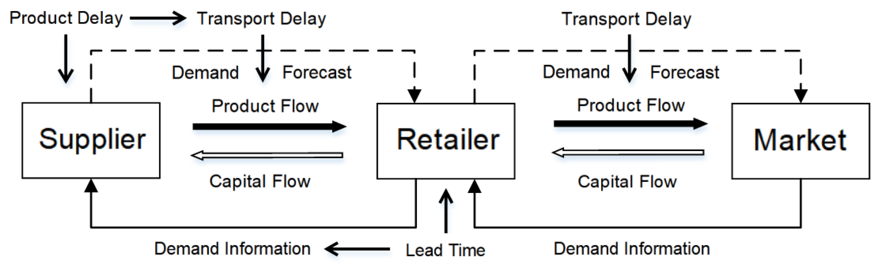
For example, FMCG supply chain market pathways are short and wide, and the operation process is cross-influenced by external market factors and internal dynamics. As the fluctuating demand for manufactured goods is highly influenced by factors such as buyer preference and ease of purchase coupled with the market penetration of imitations, consumers are prone to switching to different brands in similar products, i.e., brand loyalty is not high. Therefore, in order to maintain a certain amount of market share, manufacturers have to make frequent product upgrades to expand sales varieties, and ultimately, its value characteristics are mainly reflected in two aspects: timeliness and diversity. At the same time, since external conditions cannot be completely controlled, we pay more attention to the regulation of the internal dynamics from the supply chain. A single supply chain linking the different participants, including the supply chain network node enterprises, will be established based on factors such as quality control, cost and profitability, and other relevant considerations in selecting the object of cooperation and its relevant products. During the process of the formation of the supply chain, it is important to consider the direction of the information and financial flow from downstream to upstream of the direction, and the direction of the product flow from upstream to downstream (as in Figure 1). However, the interactive process is subject to the potential for mutual promotion and mutually beneficial outcomes but may also lead to a decline in individual firm or supply chain overall profits due to factors such as information asymmetry. The uncertainty in this internal collaboration is indicative of its internal dynamism.

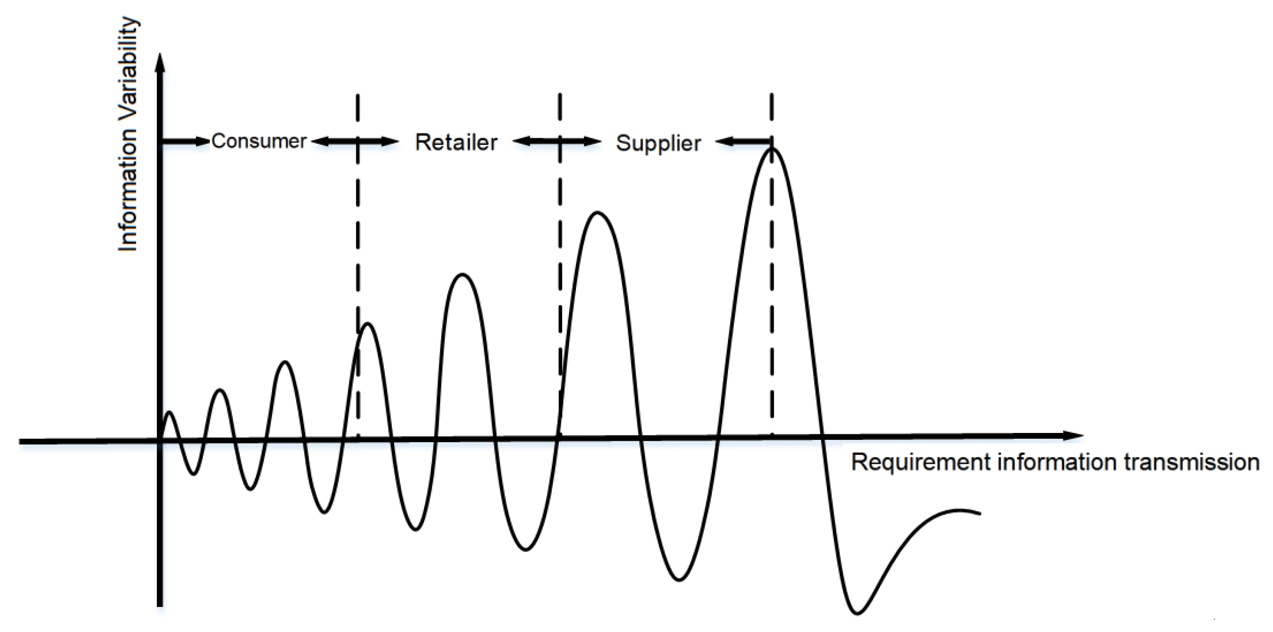
The supply chain’s dual marginal effect and bullwhip effect caused by external random demand fluctuations and upstream/downstream information asymmetry (Figure 2) are both manifestations of this internal dynamism. The double marginal effect occurs when the goals of enterprises at different nodes in the supply chain are inconsistent. By setting their own optimal solutions, products are repeatedly priced during the circulation process, ultimately leading to the disruption of supply and demand balance and poor overall supply chain efficiency. The bullwhip effect occurs when the demand information transmission of upstream and downstream enterprises in the supply chain lags behind, making it difficult for enterprises to establish reasonable inventory, resulting in increased resource waste and cost consumption, which affects the coordinated development of the supply chain.

Generally speaking, the construction of the model reflects the research idea of the researcher, and system dynamics is no exception. In this paper, the research ideas of using this method are to (1) clarify the problem and determine the system boundary; (2) put forward the dynamic hypothesis; (3) analyze the system structure and write the equations; (4) test the model; and (5) simulate and analyze. The following will be a specific study in relation to the research object of this paper.

4. Assumption Constraints and System Modeling

4.1. Basic Assumptions for Model Construction

In order to fully reflect the actual situation and simplify the model as much as possible for more accurate analysis, the following research hypotheses are made based on the research scope of the model.

Based on the coordination goal of this paper, the performance of product performance is different; furniture, electrical appliances, automobiles, and other long-cycle life products are updated and iterated quickly. However, for the retail industry, the order status of durable goods is relatively holistic and systematic, and behavioral strategies such as pre-sale and replenishment are often present in the sales process. Market competition is more of a long-term strategic nature. For daily necessities, tobacco, food and beverages, and other short-life-cycle products, they are more sensitive to short-term changes in market demand. Their market categories are richer, and their information transfer and response speed are faster. Therefore, it is more suitable to discuss the coordination of the supply chain in a short cycle. On the other hand, this paper focuses on the problem of cooperative decision making among members of a supply chain strip. The impact of too many structural disturbances should be minimized. Therefore, Assumption 1 is as follows.

Assumption 1.

The research object of this article is a secondary short-life-cycle product supply chain composed of a supplier and a retailer, and it is only a single supply chain.

Since this paper focuses on the coordination of internal members of the supply chain as well as the whole, it does not deal with the influence of special events as well as external factors in special periods. Therefore, complex market demand types are not considered, and the demand is set as a random fluctuation input. Assumption 2 is as follows.

Assumption 2.

Market demand is stochastic, with no extreme conditions such as demand interruption.

The conclusions drawn from studying relatively simple chain structures tend to have optimization and morphing potential. Therefore, the starting point of the research in this paper is set to be decentralized and the decentralized vs. centralized explored in the paper will not involve structures such as supplier-controlled inventory, joint inventory, and so on. Assumption 3 is as follows.

Assumption 3.

Inventory is set as independent inventory for suppliers and retailers, and the inventory inspection method is periodic inventory inspection.

A decentralized structure generally means that the members are only responsible for their own operations, and the benefit objectives are considered relatively individual. And it is not exactly equivalent to the meaning of centralized in the broad sense. In this paper, the centralized structure is based on the goal of optimal development of the overall efficiency of the supply chain while focusing on the coordination of the micro-structure. Among them, having sufficient consultation as well as the exchange of resources and information are the key features of the centralized style. Combined with previous studies in the literature, assumption 4 is as follows.

Assumption 4.

Centralization is achieved by incorporating information-sharing mechanisms and revenue-sharing contracts.

Simulation models tend to ignore the feasibility of realistic factors. The expected limits for equilibrium gains and the cooperation preferences of the firm’s decision makers should also have been considered. Therefore, taking into account the feedback from the research participants as well as their experiences, we limit the upper limit of revenue sharing in the contract. Assumption 5 is as follows.

Assumption 5.

Considering practical factors, the maximum sharing limit for retailers under the revenue-sharing system is 20% of their own profits.

4.2. Construction of Model System Flow Diagram

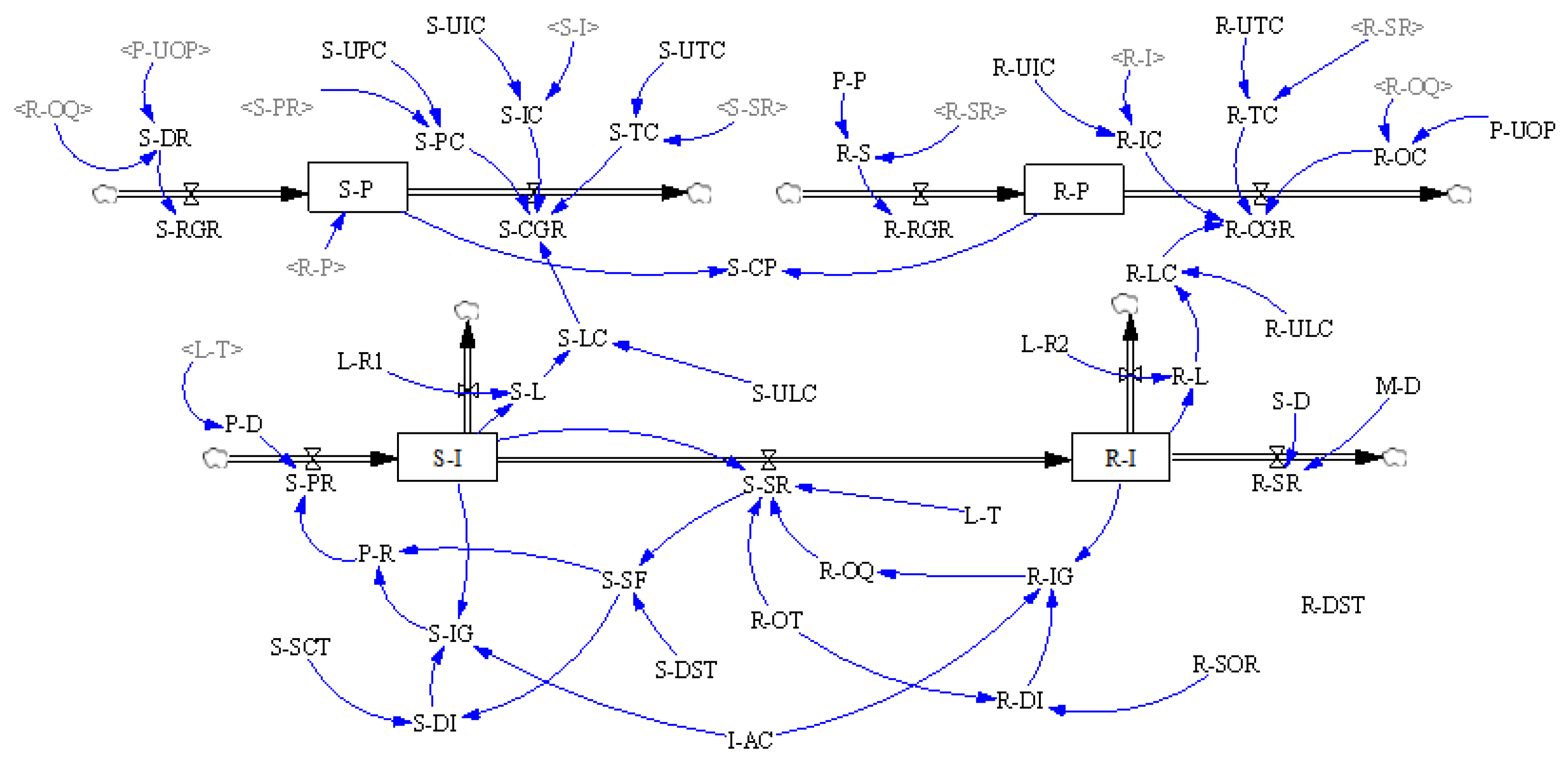
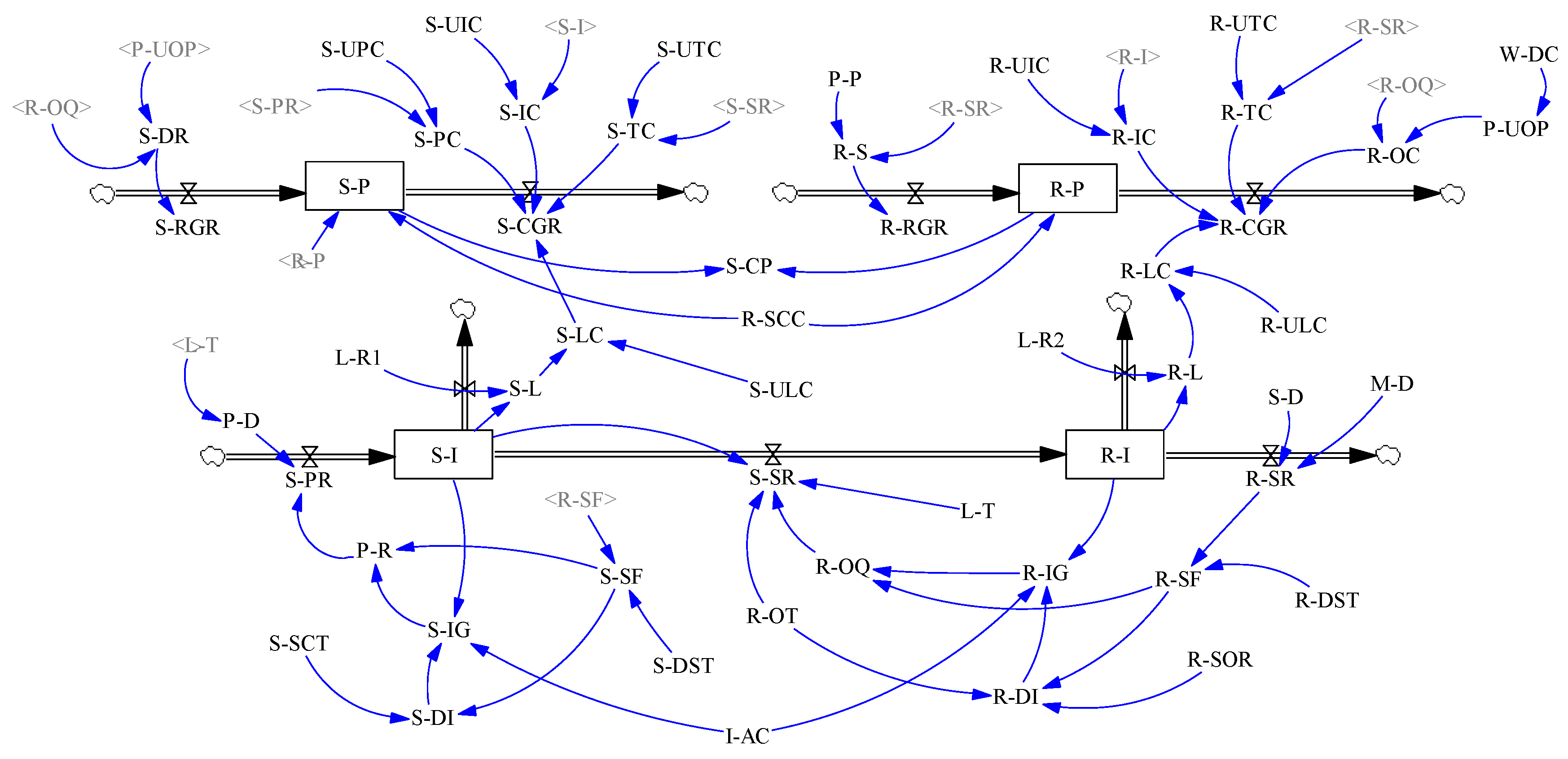
The random input of market demand and the characteristics of short inventory and fast selling of goods require retailers and suppliers to effectively reduce inventory levels and maintain stable inventory fluctuations and respond quickly to market changes, improve prediction accuracy, and stabilize the dynamic balance of input and output. Meanwhile, as the supply chain continues to develop and mature, exploring the coordinating role of time variables has gradually become a focus of research for scholars. To this end, the model introduces a time variable of order lead time internally. The system flow diagram is shown in the following Figure 3.

In decentralized decision making in the supply chain, participating members make decisions independently, and upstream behavior is often triggered by downstream decisions. Usually, upstream enterprises lack global information (such as retail customer demand patterns and information from different time points in the supply chain) and have to rely on information they can obtain, such as production efficiency, their own inventory situation, and order information issued by downstream units. The variable symbol comparison table is shown in the following

Table 1. Variable symbol comparison.

Variable Name	Symbol	Variable Name	Symbol
Supplier Inventory	S-I	Supplier Inventory Cost	S-IC
Retailer Inventory	R-I	Supplier Unit Transport Cost	S-UTC
Supplier Profit	S-P	Supplier Transport Cost	S-TC
Retailer profit	R-P	Retailer Order Time	R-OT
Supply Chain Profit	S-CP	Retailer Order Quantity	R-OQ
Supplier Purchase rate	S-PR	Lead Time	L-T
S-Shipment Rate	S-SR	Retailer Desired Inventory	R-DI
Retailer Sales Rate	R-SR	Retailer Inventory Gap	R-IG
Supplier Revenue Growth Rate	S-RGR	Retailer Sales Forecast	R-SF
Supplier Cost Growth Rate	S-CGR	Retailer Demands Smooth Time	R-DST
Retailer Revenue Growth Rate	R-RGR	Retailer Stock-out Rate	R-SOR
Retailer Cost Growth Rate	R-CGR	Market Demand	M-D
Supplier Sales Forecast	S-SF	Sales Delay	S-D
Supplier Demands Smooth Time	S-DST	Retailer Losses	R-L
Inventory Adjustment Cycle	I-AC	Loss Rate 2	L-R2
Supplier Desired Inventory	S-DI	Retailer Loss Cost	R-LC
Supplier Safety Coverage Time	S-SCT	Retailer Unit Loss Cost	R-ULC
Supplier Inventory Gap	S-IG	Product Price	P-P
Production Requirement	P-R	Retail Sales	R-S
Production Delay	P-D	Retailer Unit Inventory Cost	R-UIC
Supplier Losses	S-L	Retailer Inventory Cost	R-IC
Loss Rate 1	L-R1	Retailer Unit Transport Cost	R-UTC
Supplier Loss Cost	S-LC	Retailer Transport Cost	R-TC
Supplier Unit Loss Cost	S-ULC	Wholesale Discount Coefficient	W-DC
Supplier Delivery Revenue	S-DR	Retailer Unit Order Price	R-UOP
Supplier Unit Production Cost	S-UPC	Retailer Order Cost	R-OC
Supplier Production Cost	S-PC	Revenue Sharing Contract Coefficient	R-SCC
Supplier Unit Inventory Cost	S-UIC

.

4.3. Important Parameters and Equation Explanations

In order to ensure that the test results are in line with reality, this article takes dairy beverages in fast-moving consumer products as an example for simulation analysis. The simulation data and variable relationships included in the model refer to relevant information on dairy beverages in Z supermarket and model materials in references [12,13,14].

The model system includes three types of variables: state variables, rate variables, and general variables. There are four stocks such as S-I, R-I, etc. There are nine types of traffic such as S-PR, S-SR, etc. General variables also include auxiliary variables and constants, including 41 such as P-R, R-IG, S-IG, etc. The variable names and equation designs are shown in

Table 2. Variable equations.

Variable Type	Equation Design	Unit
State variable	S-I = INTEGER(S-PR − S-SR − S-L, initial time)	kg
	R-I = INTEGER(S-SR − R-SR − R-L, initial time)	kg
	S-P = INTEGER(S-RGR − S-CGR, initial time)	yuan
	R-P = INTEGER(R-RGR − R-CGR, initial time)	yuan
Rate variable	S-SR = IF THEN ELSE(R-OQ ≤ S-I, SMOOTH(R-OQ, L-T + R-OT), SMOOTH(S-I, L-T + R-OT))	kg/Day
	R-SR=DELAY1(M-D, S-D)	kg/Day
	S-L = S-I * L-R1	kg/Day
	R-L = R-I * L-R2	kg/Day
	S-CGR = S-PC + S-IC + S-TC + S-LC	yuan/Day
	R-CGR = R-OC + R-IC + R-TC + R-LC	yuan/Day
Auxiliary variable	M-D = RANDOM UNIFORM(200, 350, 280)	kg/Day
	R-SF = SMOOTH(R-SR, R-DST)	kg/Day
	R-DI = R-SF * R-OT * (1−R-SOR)	kg/Day
	R-IG = MAX(0, (R-DI − R-I)/I-AC)	kg/Day
	R-OQ = MAX(0, R-SF + R-IG)	kg/Day
	S-DI = S-SF * S-SCT	kg/Day
	S-IG = MAX(0, (S-DI − S-I)/I-AC)	kg/Day
	P-R = MAX(0, S-SF + S-IG)	kg/Day
	S-DR = R-UOP * R-OQ	yuan/Day
	S-PC = S-UPC * S-PR	yuan/Day
	S-IC = S-I * S-UIC	yuan/Day
	S-TC = S-UTC * S-SR	yuan/Day
	S-LC = S-L * S-ULC	yuan/Day
	S-CP = S-P + R-P	yuan/Day

below.

5. Model Simulation and Analysis

5.1. Decentralized Supply Chain Coordination

Before simulation, the model was successively tested for structural soundness and extreme conditions. For space considerations, we will not repeat them here. Firstly, consider a supply chain system with independent decision making by suppliers and retailers regarding lead time. At this point, retailers use product sales rates to make sales forecasts, while suppliers can only produce and ship products based on the orders submitted by retailers and predict sales for the next batch.

Table 3. Constant assignment table.

Constant Name	Constant Value	Unit
S-DST	2	Day
R-OT	3	Day
I-AC	4	Day
R-DST	2	Day
S-SCT	3	Day
P-D	1	Day
S-I(initial)	150	Kg
R-I(initial)	200	Kg

shows the assignment of constant variables.

The simulation cycle of the model is 100 days, with a simulation step size of 1 day. Under the condition that the above constants remain unchanged, the lead time of the retailer’s order is adjusted to 1 day (1 d), 3 days (3 d), and 5 days (5 d) to obtain the inventory situation of the supplier and retailer as follows:

(1)

Analysis of the Bullwhip Effect

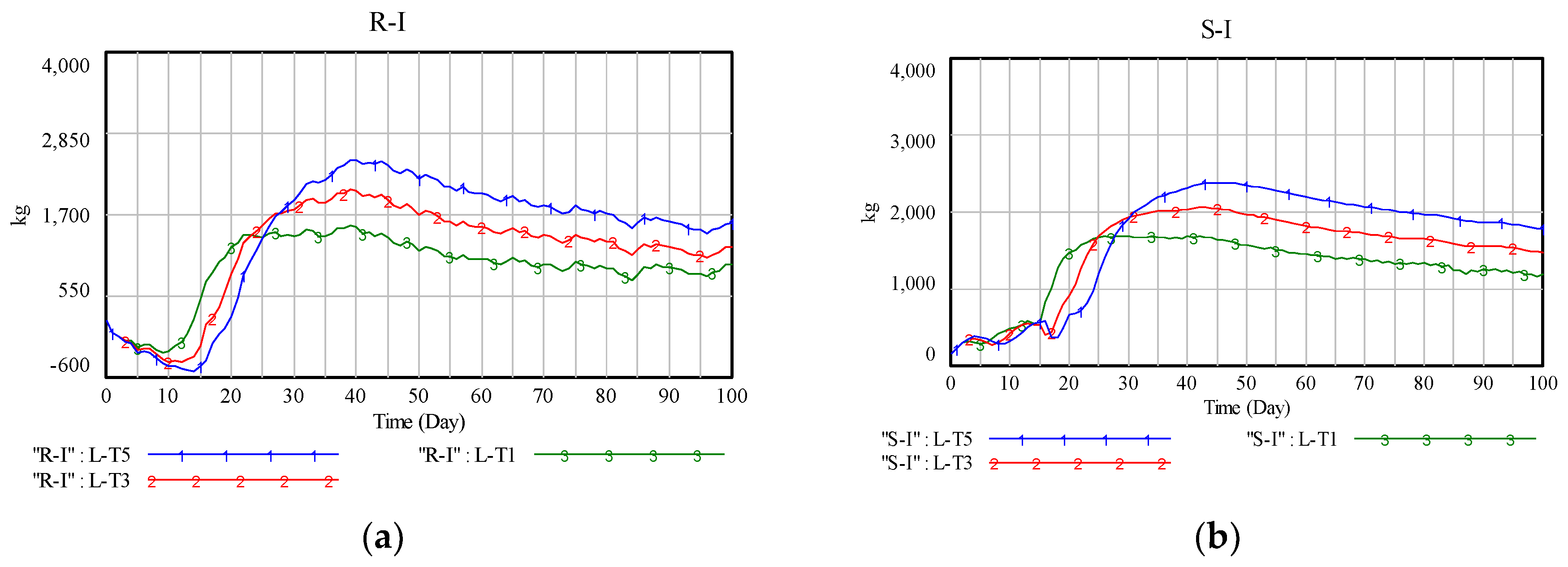
Inventory is a key factor in regulating supply and demand balance and is a state variable that members of the supply chain must focus on in various cooperation modes. A reasonable inventory level can reduce holding costs while quickly responding to market demand and reducing unnecessary waste. The fluctuation status of inventory can reflect the strength of the bullwhip effect. This section conducts a 100-day simulation analysis on the inventory level when suppliers and retailers make decentralized decisions under the influence of lead time.

It can be clearly seen from Figure 4 that in a decentralized supply chain system, the peak levels of retailer inventory with lead times of 1 d, 3 d, and 5 d are reached in 22 d, 33 d, and 40 d, respectively, while those of suppliers are 26 d, 42 d, and 46 d. Both retailer and supplier inventory will enter a stable and lower level faster as the lead time shortens. At the same time, it also reflects that the node firms in the supply chain will respond more quickly and accurately to the external demand as the lead time is compressed. The speed of stabilizing their own state also increases.

In order to better measure the impact of lead time on the “bullwhip effect”, the variance suns is used to measure the inventory fluctuation after entering the steady state. Observe that stocks under all three lead times go to a relative plateau after 40 d of simulation length. As shown in

Table 4. Supplier inventory variance sum at different lead times (decentralized supply chain).

	L-T1	L-T3	L-T5
Supplier inventory variance sum	1,195,714.23	1,765,058.86	2,139,915.70

and

Table 5. Retailer inventory variance sum at different lead times (decentralized supply chain).

	L-T1	L-T3	L-T5
Retailer inventory variance sum	1,484,498.76	3,336,775.92	4,859,699.88

, both retailers and suppliers follow the rule that the shorter the lead time, the smaller the inventory variance sum. Combined with the above findings, it can be seen that the “bullwhip effect” in decentralized decision making is mitigated with the reduction in lead time.

(2)

Analysis of double marginal effects

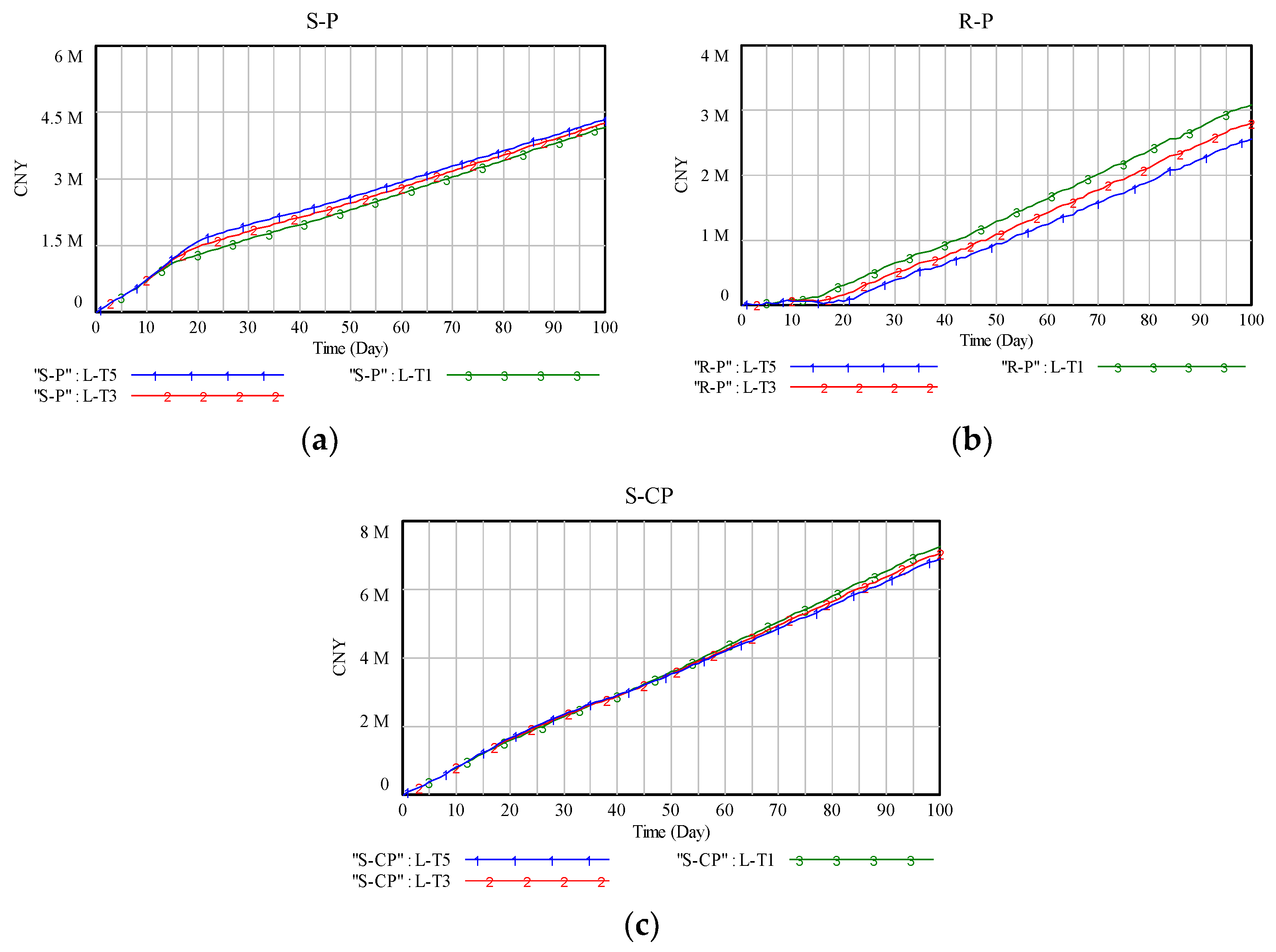
As can be seen from Figure 5, the overall profit of the supply chain shows a clear increasing trend after 15 d as the lead time is shortened. In this case, the retailer’s profit starts to rise after a short break-even period. The profit curve with a lead time of 1 d is consistently higher than that with lead times of 3 d and 5 d, and the rate of rise continues to accelerate, with the difference in profit potentials becoming progressively larger. Suppliers show the opposite trend, with shorter lead times keeping their profits at a low level. However, it is also observed that the difference between the three curves decreases over time.

In the actual supply chain system, the shortening of lead time will weaken the lag in market judgment of enterprises in the supply chain. At the same time, the sensitivity and accuracy of forecasting will be enhanced. This characteristic substantially eliminates the uncertainty of market demand or the ambiguity of excessively long lead times. It mitigates the risk of having to increase inventory holdings to cope with unforeseen events such as stock-outs. At the same time, the cost of inventory holding is also reduced with the reduction in inventory levels. Since retailers belong to the downstream enterprises of the chain, they are directly facing the customers’ demand, and the shortening of lead time has a more obvious effect of improving their operation compared with the middle and upstream enterprises. The supplier, as the source of the supply chain, is actually uncertain in the process of obtaining order information and reproducing. On one hand, the rationality of orders is strongly biased in favor of retailers, and this decentralized decision-making approach does not provide a more direct and effective way for suppliers to predict the market. On the other hand, suppliers plan production in accordance with the orders of downstream firms, and while the shortening of the lead time for ordering may mitigate the asymmetry in the information transfer process, it may also result in the inability of suppliers to reasonably set safety stock standards in the short term. The randomness of demand inputs prevents them from responding adequately to sudden changes in order levels, which may be detrimental to their short-term profits.

5.2. Centralized Supply Chain Coordination

In contrast to a decentralized supply chain, this model changes how suppliers predict the market via retailers’ orders instead of sharing retailers’ sales forecast information with suppliers. A wholesale discount factor and a revenue-sharing contract factor are introduced into the cost-income subsystem. The supplier gives the retailer a discounted price for wholesale orders, while the retailer promises to give the supplier a portion of the shared revenue after making a profit in order to improve the operational efficiency of the supply chain, harmonize the win-win relationship, and enhance the overall profitability of the supply chain.The model is shown in Figure 6.

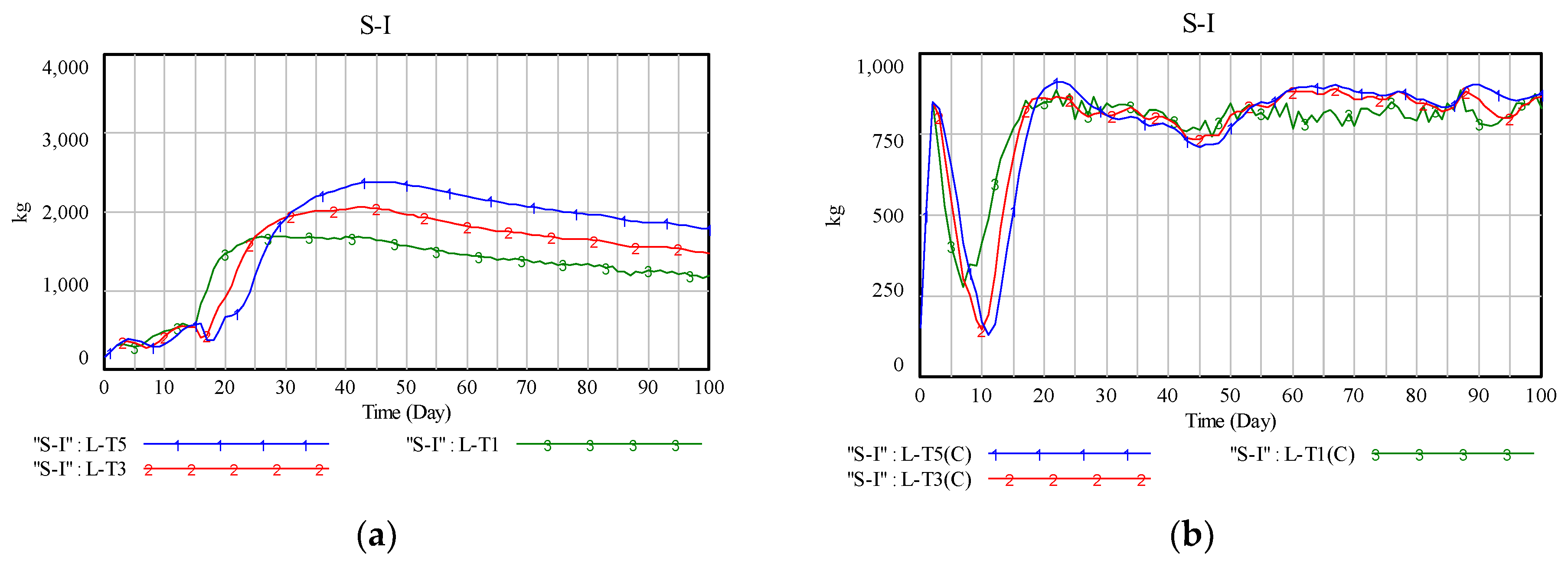
Since the demand information starts from downstream and reaches upstream via multiple levels of delayed transmission, the accuracy of the information received by the suppliers at the top of the upstream supply chain is most obviously disturbed. We observe the impact of lead time decisions on the bullwhip effect in the supply chain from the fluctuation of suppliers’ inventory. (In

Table 6. Supplier inventory variance sum at different lead times (centralized supply chain).

	L-T1	L-T3	L-T5
Supplier inventory variance sum	65,226.27	124,165.08	240,838.47

, (D) stands for decentralized decision making, and (C) stands for centralized decision making.)

In Figure 7, we can see that regardless of the length of the lead time, the inventory level of centralized suppliers is lower than that of the decentralized suppliers under the same lead time condition. This indicates that centralized decision making enables the upstream enterprises in the supply chain to obtain demand information more directly and accurately and respond quickly, and their own inventory levels can be kept low. In addition to the horizontal data comparison, the supplier inventory volatility under different lead time levels should also be considered. Here, we select the supplier inventory variance after 20 d of the centralized supply chain for comparison, as shown below:

Table 6 shows that lead time significantly affects the supply chain bullwhip effect. The longer the lead time, the larger the supplier inventory variance sum, which is manifested by the larger curve fluctuation, indicating a more serious bullwhip phenomenon. In order to ensure the coordinated operation of the supply chain, in addition to controlling the inventory level and its smooth operation, it is also necessary to mitigate the phenomenon that the overall efficiency of the supply chain is lower than the sum of the interests of both sides of the supply chain due to the lopsided pursuit of their own interests by both the supplier and the retailer—the double marginal effect. For this purpose, we compare the profits of decentralized and centralized for lead times of 1 d, 3 d, and 5 d, respectively, as shown in

Table 7. Comparison of profitability of parties with L-T1.

Time	Retailer Profit (D)	Retailer Profit (C)	Supplier Profit (D)	Supplier Profit (C)	Supply Chain Profit (D)	Supply Chain Profit (C)
10 d	82,371	282,552	706,267	474,348	788,638	756,900
20 d	296,621	672,655	1,293,040	948,545	1,589,660	1,621,200
30 d	647,070	1,057,620	1,643,840	1,455,970	2,290,910	2,513,590
40 d	927,040	1,374,020	1,963,180	1,998,000	2,890,220	3,372,020
50 d	1,292,230	1,773,400	2,300,920	2,619,700	3,593,150	4,393,100
60 d	1,642,760	2,133,700	2,671,840	3,360,170	4,314,600	5,493,880
70 d	2,009,560	2,513,740	3,045,940	4,158,260	5,055,490	6,671,990
80 d	2,383,450	2,901,030	3,410,370	5,007,320	5,793,820	7,908,350
90 d	2,742,950	3,271,580	3,794,120	5,941,920	6,537,070	9,213,500
100 d	3,090,690	3,633,620	4,164,990	6,925,260	7,255,670	10,558,900

,

Table 8. Comparison of profitability of parties with L-T3.

Time	Retailer Profit (D)	Retailer Profit (C)	Supplier Profit (D)	Supplier Profit (C)	Supply Chain Profit (D)	Supply Chain Profit (C)
10 d	71,910	280,697	719,936	472,875	791,846	753,572
20 d	152,529	653,845	1,474,070	946,289	1,626,600	1,600,130
30 d	499,741	1,017,920	1,819,920	1,448,650	2,319,660	2,466,570
40 d	756,598	1,313,140	2,128,100	1,981,960	2,884,700	3,295,100
50 d	1,095,150	1,691,040	2,453,650	2,591,660	3,548,800	4,282,700
60 d	1,421,350	2,056,890	2,813,130	3,293,590	4,234,470	5,350,480
70 d	1,766,840	2,439,950	3,176,690	4,064,340	4,943,540	6,504,290
80 d	2,121,320	2,829,140	3,531,170	4,893,800	5,652,490	7,722,940
90 d	2,474,480	3,202,740	3,894,580	5,811,170	6,369,060	9,013,900
100 d	2,811,070	3,564,930	4,253,870	6,781,780	7,064,950	10,346,700

and

Table 9. Comparison of profitability of parties with L-T5.

Time	Retailer Profit (D)	Retailer Profit (C)	Supplier Profit (D)	Supplier Profit (C)	Supply Chain Profit (D)	Supply Chain Profit (C)
10 d	64,329	280,183	729,189	470,830	793,518	751,013
20 d	59,553	647,018	1,588,410	945,736	1,647,960	1,592,750
30 d	389,344	999,712	1,969,840	1,444,430	2,359,180	2,444,150
40 d	631,794	1,281,510	2,270,370	1,973,760	2,902,160	3,255,270
50 d	946,507	1,644,840	2,584,930	2,577,160	3,531,440	4,221,990
60 d	1,248,040	1,997,140	2,932,860	3,269,720	4,180,900	5,266,860
70 d	1,571,040	2,368,660	3,285,550	4,028,320	4,856,590	6,396,970
80 d	1,905,010	2,748,040	3,629,790	4,843,490	5,534,800	7,591,530
90 d	2,239,220	3,125,240	3,983,440	5,734,290	6,222,660	8,859,530
100 d	2,558,210	3,485,330	4,333,450	6,686,510	6,891,660	10,171,800

.

The results are compared below when the lead time is 1 d: The profit of the retailer is always higher in the centralized than decentralized supply chain. The supplier has higher profits under decentralized in the early period, but after 43 d, profits under centralized exceed decentralized, and the gap gradually widens over time. The total supply chain profit is higher in centralized than decentralized after 22 d, and the gap is increasing.

The results are compared below when the lead time is 3 d: The profit of the retailer is always higher in the centralized than decentralized supply chain. The supplier has higher profits under decentralized in the early period, but after 50 d, profits under centralized exceed decentralized, and the gap gradually widens over time. The total supply chain profit is higher in centralized than decentralized supply chain after 27 d, and the gap is increasing.

The results are compared below when the lead time is 5 d. The profit of the retailer is always higher in the centralized than decentralized supply chain. The supplier has higher profits under decentralized in the early period, but after 55 d, profits under centralized exceed decentralized, and the gap gradually widens over time. The total supply chain profit is higher in centralized than decentralized supply chain after 30 d, and the gap is increasing.

Overall, it is divided into two dimensions: firstly, whether supplier, retailer, or the supply chain as a whole, the profit under the centralized mode will always be higher than the decentralized mode after a certain length of time; secondly, with the shortening of the lead time, the slopes of the profit curves of the retailer and supplier are increasing, and the profits of the suppliers and the supply chain as a whole can reach the intersection point of the two decision-making modes more quickly. This shows that centralized decision making can improve the cooperative enterprise, which not only deepens the suppliers’ willingness to cooperate but also promotes the coordinated development of the whole supply chain.

5.3. Centralized Supply Chain Coordination under Target Heterogeneity

To date, research results generated under the condition that the parameters of the revenue-sharing contract are fixed. In order to enrich the research conclusions, contribute to the cooperation and stabilization of inter-firms with higher probability, and find the optimal decision domain of the lead time, we will adjust the key parameters of the centralized decision structure in the next step. We will observe and compare the stage-by-stage profit direction of supply chain parties’ interactions to find more specific paths and countermeasures to drive the coordinated development of the supply chain.

First of all, based on the above simulation results, it can be concluded that the retailer’s profit in the simulation period is all higher than the decentralized mode when the length of the lead time is 1 d, 3 d, and 5 d for the centralized at the coefficient of a contract of 0.018 and the coefficient of wholesale discount of 0.95, and the supplier and the supply chain as a whole are also superior to the centralized in terms of profit in the long run. However, the reality is that some suppliers may mind short-term profit and loss because they do not see the future trend of profit, thus hindering the smooth achievement of the second level of cooperation mode; for this reason, this paper uses Tpd (meaning: time of profit disadvantage) to indicate the time when the supplier profit under the centralized mode at the beginning of the simulation is briefly lower than that under the decentralized mode. Then, the further “coordination condition” is to keep the retailer’s profit level within the permissible range and simultaneously shorten the Tpd to help the supplier obtain a satisfactory level of benefits as soon as possible. In other words, combining contract coefficients and wholesale discount coefficients to shorten the Tpd to a suitable area will be the key to stabilizing the cooperative relationship.

In the parameter exploration stage, the following laws are found: ① when the wholesale discount coefficient is set to 0.8, it is necessary to adjust the coefficient of the revenue-sharing contract to about 0.3 at the same time in order to achieve the above coordination conditions, but at this time, the assumptions are no longer satisfied; ② in the value domain, the larger the coefficient of revenue-sharing contract and the coefficient of wholesale discount are, the better the coordination effect is. Therefore, based on the research pattern and assumption constraints, we set the wholesale discount coefficient between 0.85 and 0.95 and the shared covenant coefficient between 0.005 and 0.2 to determine the adjustment range. (Note: the following for example (a, b) is interpreted as the case where the wholesale discount coefficient is (a) while the revenue sharing coefficient is (b)). The simulation results are shown below.

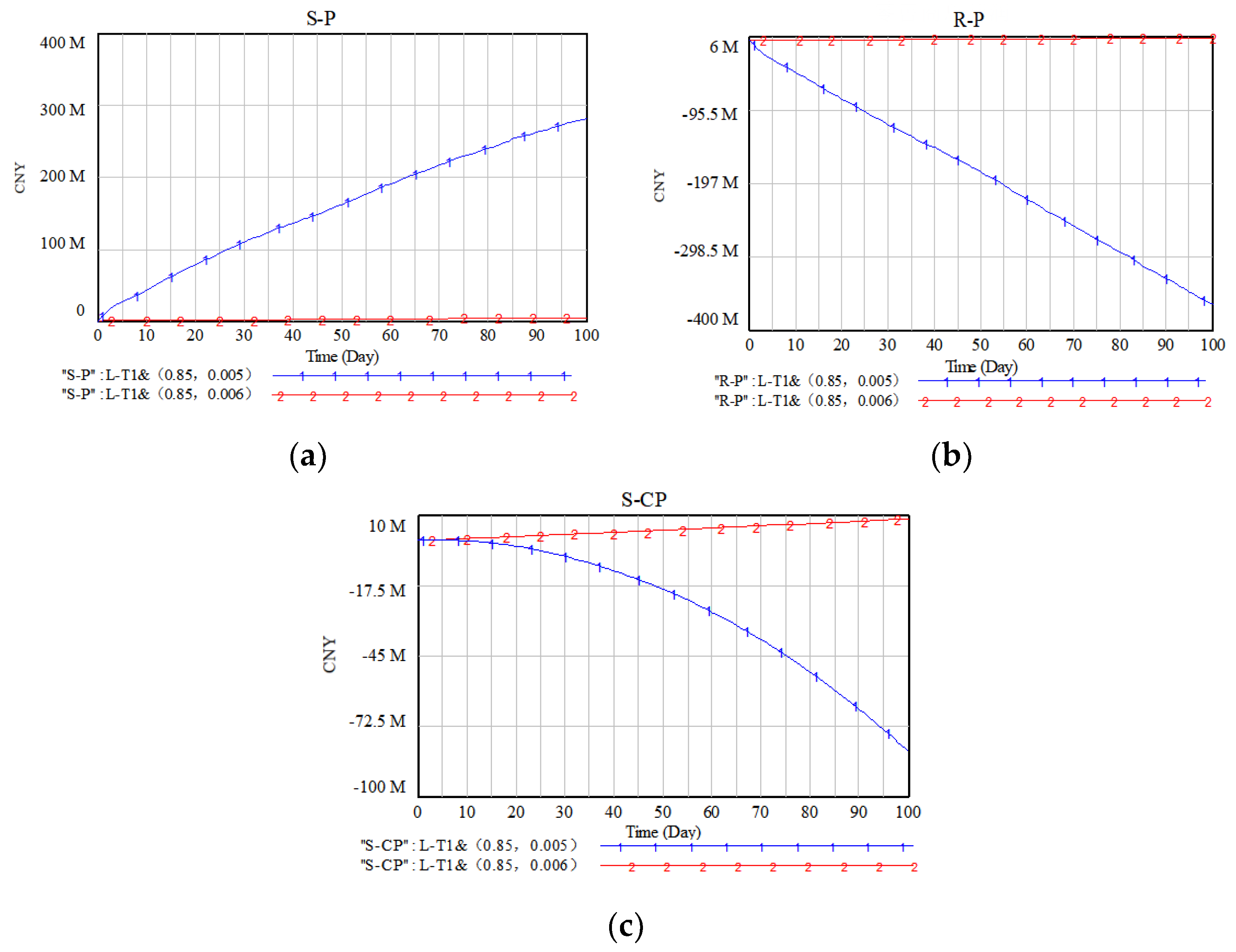
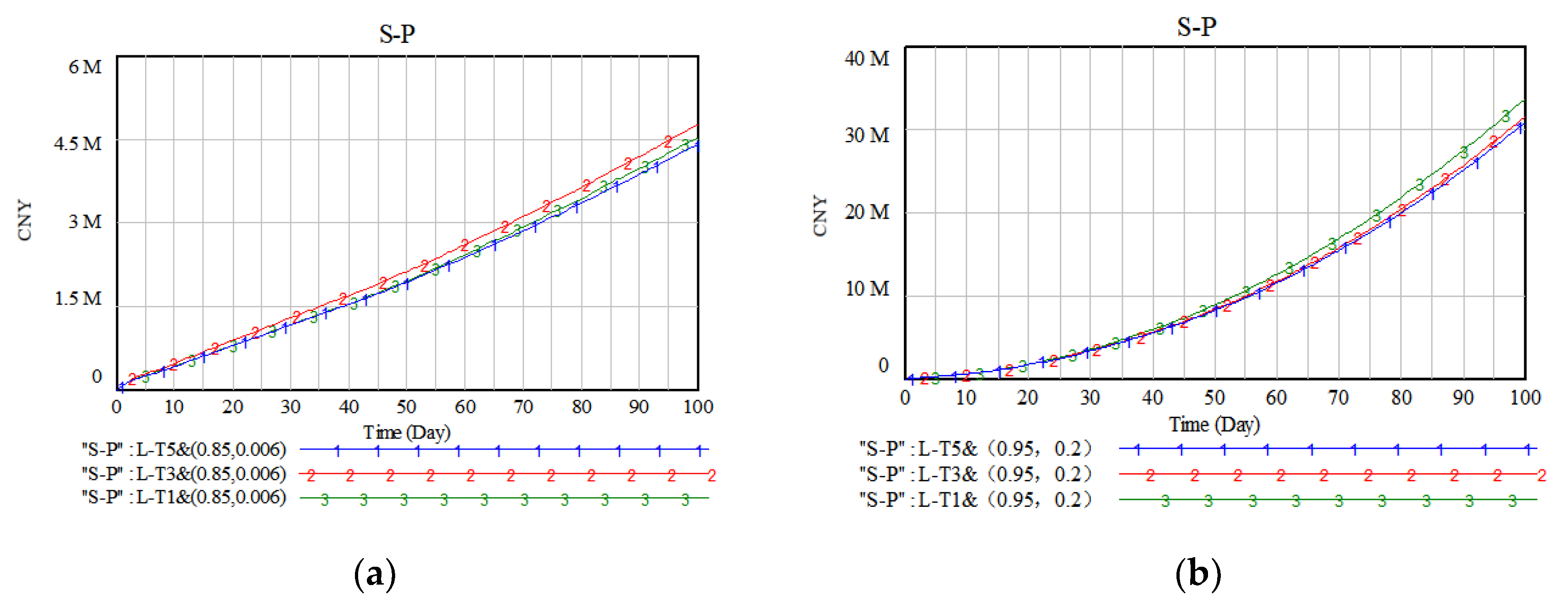
Step 1: As shown in Figure 8, Iconsider the case where the lead time is 1 d, and the parameter combination is (0.85, 0.005). It is observed that the curve declines day by day, and the supply chain profit system collapses completely. When the coefficient of the revenue-sharing contract is adjusted to 0.006, the system returns to normal and is in the “coordination condition” state. This indicates a critical point between the two combinations that affects the system’s stability. According to research rule ②, the lower limit of parameter combination to reach the “coordination condition” is (0.85, 0.006).

Step 2: According to Law ②, when the wholesale discount coefficient is set to 0.95,

Table 10. Retailer’s profit under different decision structure and parameter combinations with L-T1.

Simulation Time	Centralized Mode		Decentralized Mode
	(0.95,0.16)	(0.95,0.17)
1 d	18,831	18,607	18,822
50 d	1,516,960	1,398,900	1,491,120
100 d	3,108,190	3,071,180	3,090,690

shows that the retailer’s profit level is lower than the decentralized decision under the conditions of 1 d lead time and the parameter combination of (0.95, 0.17), which means that this scheme harms the retailer’s profit and is not adopted. By adjusting the gain-sharing contract factor to 0.16, the system returns to normal and is in a “harmonized state”. At this point, it is found that when the wholesale discount coefficient takes the maximum value of 0.95 in the range, the contractual coordination coefficient of 0.16 < 0.2 (assuming constraints), and for the time being, it is not possible to use (0.95,0.16) as the upper limit of parameter combinations. Since other parameter combinations such as (0.94, 0.17) may result in better supplier profitability under the “coordination condition”, the parameter combinations need to be re-selected for comparative analysis.

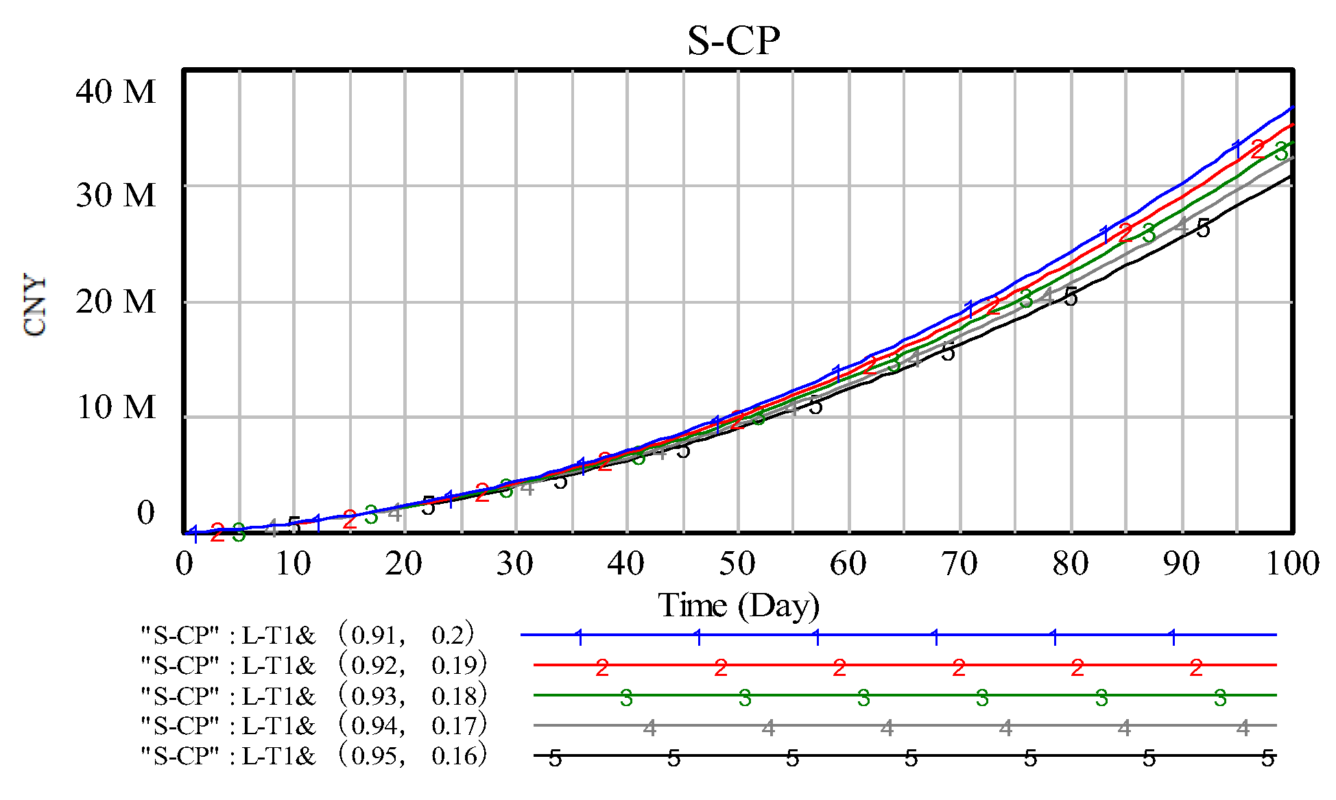
Step 3: Repeat step 2 with the help of the “dichotomy” research idea and adjust the five parameter combinations as shown in Figure 9 without harming the interests of retailers and the supply chain as a whole. Due to the influence of assumption constraints, once the coefficient of revenue sharing contract in the parameter combinations reaches 0.2, no further adjustment can be made, and the upper limit of the parameter combinations to reach the “coordination conditions” is finally determined to be (0.91,0.2).

Step 4: Via steps 1, 2, and 3, it can be finally determined that when the lead time is 1 d, the parameter combinations that can reach the “coordination conditions” under centralized mode are ((0.85,0.006), (0.91,0.2)).

Similarly, we can find the domain of values of parameter combinations when the lead time is 3 d and 5 d based on the above three steps as ((0.85,0.006), (0.95,0.2)) and ((0.85,0.006), (0.95,0.2)), respectively.

According to the above conclusion, the Tpd and the supplier’s profit when the lead time is 1 d, 3 d, and 5 d are compared and analyzed, and the lower limit of the parameter combination is called “before improvement”, and the upper limit is called “after improvement”. The simulation results are shown in the figure below.

From

Table 11. Tpd values at different lead times.

Lead Time	Tpd (Before Improvement)	Tpd (After Improvement)	Tpd (Gap)
L-T1	80 d	15 d	65 d
L-T3	75 d	17 d	58 d
L-T5	97 d	19 d	78 d

, it can be seen that when the lead time is 1 d, the shortest Tpd of the parameter combination “after improvement” is 15 d, which means that the supplier’s profit can reach the intersection of centralized and decentralized mode the fastest when the lead time is 1 d. Meanwhile, via the difference in Tpd, we find that the smallest change in the direction of the supplier’s profit before and after the improvement in parameter combinations is when the lead time is 3 d, with a Tpd difference of 58 d, and the largest change in the direction is when the lead time is 5 d, with a Tpd difference of 78 d.

As shown in Figure 10, the trend of profit level to suppliers before and after the improvement is different; in order to further study the improvement in parameter combinations under different lead times to bring different impact effects on suppliers and the supply chain as a whole, the statistics are as follows:

Table 12. Supplier’s profit at different lead times before and after improvement.

Simulation Time	Before Improvement			After Improvement
	L-T1	L-T3	L-T5	L-T1	L-T3	L-T5
20 d	791,911	882,397	790,631	1,762,700	1,722,700	1,718,040
50 d	1,941,820	2,116,960	1,927,250	8,892,750	8,360,210	8,234,390
80 d	3,420,190	3,619,750	3,338,640	21,818,200	20,376,000	19,934,200
100 d	4,519,960	4,746,310	4,400,190	33,660,100	31,516,700	30,802,000

and

Table 13. Supply chain profit at different lead times before and after improvement.

Simulation Time	Before Improvement			After Improvement
	L-T1	L-T3	L-T5	L-T1	L-T3	L-T5
20 d	1,569,780	1,544,230	1,542,440	2,341,910	2,255,370	2,245,150
50 d	3,953,970	3,828,670	3,809,170	10,407,400	9,737,840	9,574,380
80 d	6,706,270	6,483,460	6,465,390	24,294,100	22,680,800	22,172,900
100 d	8,634,270	8,354,800	8,357,860	36,760,700	34,420,900	33,641,300

show the specific data of the profit value of the supplier and the whole supply chain before and after the improvement in the parameter combination, and it is found via the comparative analysis that ① before the improvement in the parameter combination, the profit level of the supplier in each stage of the simulation cycle is not strictly in accordance with the trend of the higher profit level of the supplier with the shorter lead time, and the profit level is the highest in the case of the lead time of 3 d. For the overall profit level of the supply chain, there is also a disorder in the later stage when the lead time is 5 d, which is higher than 3 d. ② With the parameter combination “after improvement”, both the supplier and the whole supply chain profits at each stage of the simulation period increase with the shortening of lead time. ③ The supplier’s profit level and the supply chain’s overall profit level after improvement are much higher than before improvement, and the advantage gradually increases with the simulation time.

Table 14. Supply chain profit at different lead times before and after improvement.

Simulation Time	Before Improvement			Decentralized Mode
	L-T1	L-T3	L-T5	L-T1	L-T3	L-T5
20 d	1,569,780	1,544,230	1,542,440	1,589,660	1,626,600	1,647,960
50 d	3,953,970	3,828,670	3,809,170	3,593,150	3,548,800	3,531,440
80 d	6,706,270	6,483,460	6,465,390	5,793,820	5,652,490	5,534,800
100 d	8,634,270	8,354,800	8,357,860	7,255,670	7,064,950	6,891,660

compares the total profit of the supply chain under centralized decision making and decentralized decision making when the lower limit of parameter combination is taken. It finds that, regardless of whether the lead time is 1 d, 3 d, or 5 d, the total profit of the supply chain is higher under the decentralized mode when compared with the centralized mode “before improvement”. However, there is a short period of time in the early stage, but the overall point of view is still in a disadvantageous position. It is further validated from the perspective of the coordinated supply chain to verify the feasibility of the centralized mode under the decision-making domain of parameter combination.

In summary, there are two models of cooperation for the centralized supply chain oriented to goal heterogeneity.

(1)

With cooperative stability as the primary goal

This model aims to help the supplier obtain a stronger willingness to cooperate, which can weaken part of the retailer’s revenue at an appropriate range. In the pre-cooperation period between the supplier and the retailer, the order lead time is compressed to 1 d, while the parameter combination is set to (0.91.0.2) so that the supplier’s Tpd value is the shortest. In this state, the retailer’s profit is still higher than that of a decentralized company, while the supplier’s benefit reaches a satisfactory level in the shortest time, which maximizes the stability of the cooperative relationship. However, the first middle stage will cause the retailer to be unable to achieve more profits due to the adoption of centralized decision-making mechanisms that are more favorable for suppliers to participate in the cooperation. Therefore, the decision-making model can be adjusted when the profit level of the supplier is higher than the decentralized decision making after entering the middle stage of cooperation. According to the duration of cooperation, within the scope of “coordination conditions”, the coefficient of revenue sharing contract should be reduced, and the wholesale discount coefficient should be increased, in order to regulate the profit leverage; the benefits of the advantage will gradually shift to the retailer, mobilizing the enthusiasm of both parties to cooperate. At this time, the overall profit level of the supply chain is also relatively high, and the two sides will maintain a friendly situation of “profitable, win-win cooperation”, which is conducive to the overall coordinated and sustainable development of the supply chain.

For FMCG supply chains, such as dairy products, there may be challenges in adopting such a cooperative model. Prior to profit leverage, retailers were in a relatively passive position in the partnership. Pricing was less flexible and could not be changed at will in response to real-time market changes due to the strategic goal of partnering first. For example, stepping outside of the hypothetical constraints, the retailer is most likely to be at the secondary crossroads of the horizontal chain due to the wide and short distribution channels of FMCG. When unexpected events occur, the cooperation mode of the chain may affect the adjustment of the overall strategic layout of the dairy enterprise. Therefore, before the cooperation is reached, it should be matched with detailed market research data and contingency plans. So, FMCG retailers can not only coordinate in the vertical chain but also in the fierce horizontal market, competition can still stand firm.

(2)

With balanced development with benefits as the primary goal

This model aims to achieve satisfactory benefits for both the supplier and the retailer under centralized decision making and only ensures that the supplier’s profit level is higher than that of decentralized decision making. Considering the possibility that retailers may not be willing to give up part of their profits in order to have a higher probability of cooperation, the effect of the Tpd value is not considered in the first place. Via the study, during the period of cooperation between suppliers and retailers, a variety of parameter combinations within the range of “coordination conditions” can be selected, based on which the overall profit level of the supply chain is fully considered. It is found that when the lead time is 1 d, and the parameter combinations take the values around the lower limit, in the pre-simulation period, there is a short period of time that is lower than the total profit of the supply chain under decentralized decision making, and as the lead time increases, the time of this situation will be longer. In order to shorten this time and consider the respective profits of suppliers and retailers, it is more reasonable to choose a lead time of 1 d and take the value of the parameter combination interval. In this way, it can ensure the benefit level of suppliers and retailers and promote the coordinated development of the supply chain as a whole.

Unlike the cooperative-led model, this model emphasizes autonomy while ensuring that the overall efficiency of the supply chain is optimized. The practical challenges are therefore different. Since the focus is more on self-efficiency, at the micro level, the degree of information sharing about the retailer’s operations and the value of the interval for the combination of the above parameters will depend on the firm’s managerial preference decisions. The assumption that firms possess overly rational traits may weaken the degree of information sharing. However, the cooperative goal of overall profit optimization cannot be violated, in which case the retailer may need to adjust the thresholds of the parameter combinations, and the selection of the interval values may affect the retailer’s original profit advantage. Therefore, in-depth discussions on the types as well as the modalities of centralized cooperation models may be worth investigating in order to address the challenges.

6. Conclusions

In this paper, with the help of Vensim software, a system dynamics simulation study was conducted to investigate the coordination problem of decentralized and centralized supply chains under the influence of lead time, and the following conclusions were found:

(1)

The decentralized mode of the secondary supply chain composed of suppliers and retailers slowed down the bullwhip effect in the process of lead time shortening, and the overall profit is gradually optimized. However, there is a localized situation that is not conducive to cooperation and stability, which is manifested in the fact that the supplier’s profit decreases with the shortening of lead time. This change is contrary to the trend of retailers and the supply chain as a whole, i.e., with the shortening of lead time, the decision-making orientation of all parties in the decentralized supply chain is inconsistent, and the supply chain coordination is ineffective.

(2)

The centralized approach is more effective than the decentralized one in mitigating the bullwhip and double marginal effects. Moreover, the centralized approach not only conforms to the rule that the shorter the lead time, the more coordinated the supply chain as a whole is, but also eliminates the unfavorable factors that may lead to unsuccessful cooperation among local members in the decentralized approach, which positively promotes win-win cooperation between suppliers and retailers as well as the stability of the supply chain’s long-term sustainable development.

(3)

After comparing the centralized and decentralized approaches, it is found that the parameter combinations of the centralized contractual coordination mechanism need to be within the appropriate range of values in order to achieve the coordination effect. After repeated testing of the adjustment variables, we find the parameter combinations under different lead times. Furthermore, via comparison, it is found that with the shortening of the lead time, there are parameter combinations in the parameter range that enable suppliers to obtain a satisfactory level of benefits faster, i.e., the shorter the lead time, the higher the probability of stabilizing the situation of cooperation. In addition, based on the profit development trajectory of suppliers, retailers, and the whole supply chain, and the heterogeneous demand within the supply chain, we find a coordinated development path based on the primary goal of “cooperative stabilization” or “balanced effect”.

The supply chain coordination model in this paper also discusses the cooperative behavior of suppliers and retailers after random demand inputs from the market from a micro perspective. It can be seen that the reduction in lead time is a double-edged sword. Just making unilateral adjustments is not necessarily favorable. The supply chain benefits can only be accomplished with a reasonable decision-making structure. Therefore, it is recommended that managers should have a detailed and sufficient knowledge of the overall operation structure of the supply chain and their own development status when considering the strategic choice of the time factor. In addition, the study concludes that improving the transmission speed of information is conducive to the consistency of supply chain coordination and development goals. Whether as a supplier or retailer, in the actual supply chain operation process, we should pay attention to the mastery of order information at all levels. The research content of enterprises should not only focus on the market situation, but also on the relevance of upstream and downstream docking units. This is important to enhance their own chain embeddedness as well as survival position. In the exploration of revenue-sharing contracts, we find that suppliers and retailers are generally fully rational. The balance of responsibilities and benefits is frequently considered by managers. In choosing the appropriate revenue-sharing parameters, state policy, and concepts, management personnel from all parties should increase their frequency of communication. After a real-time understanding of the global impact of market changes, the parameters should be revised to the extent allowed by all parties. Tentative behavior should be avoided to prevent causing a backlash of two uncoordinated effects. As it is often said, competition and cooperation come hand in hand, and the period is full of games. But only with the overall coordination of the supply chain being the goal to operate their own units can this appear to reach a win-win path.

The limitations of this paper and future research directions are as follows:

(1)

In the discussion of decentralized vs. centralized, there should be more discussion on several types of centralized decision making, pointing out the advantages and disadvantages and other different conclusions. Maybe in the future research can be further refined the centralized research.

(2)

Since this paper only considers the influencing role of lead time, it does not address issues such as multi-cycle environment and time compression cost. Scholars often ignore issues such as the cycle correlation of information and updating mechanisms when considering supply and demand change studies. Setting the length of the study to be multi-cycle is the only way to achieve satisfactory and real results under the influence of multi-node change factors. Dynamic pricing, multi-cycle inventory, and other research combined with the lead time have to be studied in depth.

(3)

The model construction of this paper is limited to the proposed assumptions, and there is still a big gap between the structure and comprehensiveness of the variables covered by the model and the reality. With the development of economic globalization, the supply chain structure has become more and more complex, often not limited to parallel supply chain competition. The situation of overlapping nodes between supply chains is increasing. And the connotation of outsourcing services is becoming more and more broad, which gives supply chain managers stronger control over demand information. Extending the boundary of the theoretical system to include richer elements has yet to be studied.

References

- Ye, F.; Xu, X. Cost allocation model for optimizing supply chain inventory with controllable lead time. Comput. Ind. Eng. 2010, 59, 93–99. [Google Scholar]
- Li, Y.; Xu, X.; Ye, F. Supply chain coordination model with controllable lead time and service level constraint. Comput. Ind. Eng. 2011, 61, 858–864. [Google Scholar] [CrossRef]
- Yang, H.; Peng, J. Coordinating a fresh-product supply chain with demand information updating: Hema Fresh O2O platform. RAIRO-Oper. Res. 2021, 55, 285–318. [Google Scholar] [CrossRef]
- Wu, Q.; Zhu, J.; Cheng, Y. The effect of cross-organizational governance on supply chain resilience: A mediating and moderating model. J. Purch. Supply Manag. 2023, 29, 100817. [Google Scholar] [CrossRef]
- Nguyen, T.-H.; Wright, M. Capacity and lead-time management when demand for service is seasonal and lead-time sensitive. Eur. J. Oper. Res. 2015, 247, 588–595. [Google Scholar] [CrossRef]
- Axsäter, S. Optimization of order-up-to-s policies in two-echelon inventory systems with periodic review. Nav. Res. Logist. (NRL) 1993, 40, 245–253. [Google Scholar]
- Axsäter, S. Approximate evaluation of batch-ordering policies for a one-warehouse, N non-identical retailer system under compound poisson demand. Nav. Res. Logist. (NRL) 1995, 42, 807–819. [Google Scholar] [CrossRef]
- Chatfield, D.C.; Kim, J.G.; Harrison, T.P.; Hayya, J.C. The bullwhip effect—Impact of stochastic lead time, information quality, and information sharing: A simulation study. Prod. Oper. Manag. 2004, 13, 340–353. [Google Scholar] [CrossRef]
- Boute, R.N.; Disney, S.M.; Lambrecht, M.R.; van Houdt, B. Designing replenishment rules in a two-echelon supply chain with a flexible or an inflexible capacity strategy. Int. J. Prod. Econ. 2009, 119, 187–198. [Google Scholar]
- Abginehchi, S.; Farahani, R.Z. Modeling and analysis for determining optimal suppliers under stochastic lead times. Appl. Math. Model. 2010, 34, 1311–1328. [Google Scholar]
- Huang, Y.-S.; Su, W.-J.; Lin, Z.-L. A study on lead-time discount coordination for deteriorating products. Eur. J. Oper. Res. 2011, 215, 358–366. [Google Scholar] [CrossRef]
- Glock, C.H.; Rekik, Y.; Ries, J.M. A coordination mechanism for supply chains with capacity expansions and order-dependent lead times. Eur. J. Oper. Res. 2020, 285, 247–262. [Google Scholar] [CrossRef]
- Giri, B.C.; Roy, B. Modelling supply chain inventory system with controllable lead time under price-dependent demand. Int. J. Adv. Manuf. Technol. 2016, 84, 1861–1871. [Google Scholar]
- Fander, A.; Yaghoubi, S.; Asl-Najafi, J. Chemical supply chain coordination based on technology level and lead-time considerations. RAIRO-Oper. Res. 2021, 55, 793–810. [Google Scholar]
- Li, Y.; Xu, X.; Zhao, X.; Yeung, J.H.; Ye, F. Supply chain coordination with controllable lead time and asymmetric information. Eur. J. Oper. Res. 2012, 217, 108–119. [Google Scholar] [CrossRef]
- Jha, J.K.; Shanker, K. Single-vendor multi-buyer integrated production-inventory model with controllable lead time and service level constraints. Appl. Math. Model. 2013, 37, 1753–1767. [Google Scholar]
- Modak, N.M.; Kelle, P. Managing a dual-channel supply chain under price and delivery-time dependent stochastic demand. Eur. J. Oper. Res. 2019, 272, 147–161. [Google Scholar]
- Sarkar, S.; Tiwari, S.; Giri, B.C. Impact of uncertain demand and lead-time reduction on two-echelon supply chain. Ann. Oper. Res. 2022, 315, 2027–2055. [Google Scholar] [CrossRef]
- Kar, S.; Jha, K.N. Investigation into lead time of construction materials and influencing factors. J. Constr. Eng. Manag. 2021, 147, 04020177. [Google Scholar]
- Karthick, B.; Uthayakumar, R. A two-tier supply chain model under two distributions with MTTF, rework, variable production rate and lead time. J. Manag. Anal. 2022, 9, 532–558. [Google Scholar] [CrossRef]
- Graves, S.C. How to think about planned lead times. Int. J. Prod. Res. 2022, 60, 231–241. [Google Scholar] [CrossRef]
- Thürer, M.; Fernandes, N.O.; Haeussler, S.; Stevenson, M. Dynamic planned lead times in production planning and control systems: Does the lead time syndrome matter? Int. J. Prod. Res. 2023, 61, 1268–1282. [Google Scholar] [CrossRef]
- El Mehdi, E.R.; Ilyas, H.; François, S. Incremental LNS framework for integrated production, inventory, and vessel scheduling: Application to a global supply chain. Omega 2023, 116, 102821. [Google Scholar]
- Qiu, R.; Sun, Y.; Sun, M. A robust optimization approach for multi-product inventory management in a dual-channel warehouse under demand uncertainties. Omega 2022, 109, 102591. [Google Scholar] [CrossRef]
- Berling, P.; Johansson, L.; Marklund, J. Controlling inventories in omni/multi-channel distribution systems with variable customer order-sizes. Omega 2023, 114, 102745. [Google Scholar] [CrossRef]
- Salcedo, C.A.; Hernandez, A.I.; Vilanova, R.; Cuartas, J.H. Inventory control of supply chains: Mitigating the bullwhip effect by centralized and decentralized Internal Model Control approaches. Eur. J. Oper. Res. 2013, 224, 261–272. [Google Scholar] [CrossRef]
- Hassanzadeh, A.; Jafarian, A.; Amiri, M. Modeling and analysis of the causes of bullwhip effect in centralized and decentralized supply chain using response surface method. Appl. Math. Model. 2014, 38, 2353–2365. [Google Scholar]
- Goodarzi, M.; Makvandi, P.; Saen, R.F.; Sagheb, M.D. What are causes of cash flow bullwhip effect in centralized and decentralized supply chains? Appl. Math. Model. 2017, 44, 640–654. [Google Scholar]
- Yin, X. Measuring the bullwhip effect with market competition among retailers: A simulation study. Comput. Oper. Res. 2021, 132, 105341. [Google Scholar]
- Lee, S.; Park, S.J.; Seshadri, S. Variations of the bullwhip effect across foreign subsidiaries. Manuf. Serv. Oper. Manag. 2023, 25, 1–18. [Google Scholar] [CrossRef]
- Brauch, M.; Größler, A. Holistic versus analytic thinking orientation and its relationship to the bullwhip effect. Syst. Dyn. Rev. 2022, 38, 121–134. [Google Scholar] [CrossRef]
- Cachon, G.P. Supply chain coordination with contracts. Handb. Oper. Res. Manag. Sci. 2003, 11, 227–339. [Google Scholar]
- Liu, Y.; Xu, Q.; Liu, Z. A coordination mechanism through value-added profit distribution in a supply chain considering corporate social responsibility. Manag. Decis. Econ. 2020, 41, 586–598. [Google Scholar] [CrossRef]
- Zhang, X.; Wang, H.; Zhao, X.; Wu, D. Return decision model of the manufacturer-leading dual-channel supply chain. Math. Probl. Eng. 2020, 2020, 8864672. [Google Scholar] [CrossRef]
- Wang, D.; Wang, Z.; Zhang, B.; Zhu, L. Vendor-managed inventory supply chain coordination based on commitment-penalty contracts with bilateral asymmetric information. Enterp. Inf. Syst. 2022, 16, 508–525. [Google Scholar] [CrossRef]
Figure 1.
Model structure analysis diagram.
Figure 2.
“Bullwhip effect” in the supply chain.
Figure 3.
Decentralized supply chain system flow diagram.
Figure 4.
The inventory under a decentralized mode, considering the influence of lead time. (a) The inventory of retailer. (b) The inventory of supplier.
Figure 5.
Profitability of members in a decentralized supply chain. (a) The profits of the retailer. (b) The profits of the supplier. (c) The profits of the supply chain.
Figure 6.
Centralized supply chain system flow diagram.
Figure 7.
Supplier inventory under different modes. (a) Decentralized mode. (b) Centralized mode.
Figure 8.
The profits under the parameter combination (0.85, 0.005) and (0.85, 0.006). (a) The profits of the retailer. (b) The profits of the supplier. (c) The profits of the supply chain.
Figure 9.
Supplier’s profit for different parameter combinations.
Figure 10.
Supplier’s profit with different lead times. (a) before improvement; (b) after improvement.