A Novel DGM(1, N) Model with Interval Grey Action Quantity and Its Application for Forecasting Hydroelectricity Consumption of China

Abstract

This paper addresses the issue of the conventional DGM(1, N) model’s prediction results not taking into account the grey system theory pri1nciple of the “non-uniqueness of solutions”. Firstly, before presenting the interval grey action quantity, the practical significance of grey action quantity is examined. In the DGM(1, N) model, the grey action quantity is transformed into an interval grey action quantity. Then, the calculation of the parameters uses the least squares method. A DGM(1, N, ${\otimes }_c$) model containing interval grey action is then built, and meanwhile, the program code for DGM(1, N, ${\otimes }_c$) is provided. Lastly, the aforementioned model is used to forecast the hydroelectricity consumption of China. The findings indicate that it produces more rational outcomes than the traditional DGM(1, N) model. Overall, the research carries significant pragmatic implications for broadening the conceptual underpinnings of multivariate grey forecasting models and enhancing their structural arrangement.

1. Introduction

As the global phenomenon of the greenhouse effect continues to escalate, tackling climate change has become an expeditious concern for nations worldwide [1]. To this end, the Chinese government announced “Opinions on Fully and Accurately Implementing the New Development Concept and Doing a Good Job in Carbon Peak and Carbon Neutrality Work” in October 2021. This policy delineates the dual carbon objectives of accomplishing carbon neutrality by 2060 and carbon peaking by 2030. In this context, hydroelectricity signifies a propitious and valuable option for supporting sustainable development strategies due to its status as a clean and renewable energy source with abundant resources, mature technology, and a reliable operation [2]. Hydroelectricity consumption is an essential basis for water resource planning, development, and scheduling. Therefore, a rational and precise prognostication of hydroelectricity consumption can furnish a hydroelectricity resource development system with a reference point for planning, policy formulation, and other pertinent considerations.

According to existing research, the forecasting models of hydroelectricity consumption may be divided into two principal categories, namely statistical methods and machine learning techniques. These statistical models comprise ARIMA and its improvements [3,4], fuzzy Bayesian methods [5], and multiple regression models [6]. Machine learning approaches, such as artificial neural network models [7] and SVM [8], are also commonly utilized for hydroelectricity generation and consumption forecasting. While both statistical and machine learning models have significantly improved forecasting accuracy, they necessitate data distributions that conform to model assumptions and require extensive sample data. However, in real life, the cost and time constraints of data collection sometimes make it difficult to obtain sufficient data, and the grey system theory adequately addresses the problem of modeling data from a limited sample size.

The grey system theory is an original Chinese doctrine created by Professor Deng, which focuses on “small data, poor information” uncertainty systems, where “some information is known, and some information is unknown” [9]. Scholars typically use multivariate grey forecasting models to model predictions for real-world forecasting problems, with the systematic variables being influenced by multiple factors [10]. The multivariate grey prediction model, which treats all unknown elements as grey quantities and all known factors as drivers of a system’s behavior, holds vital significance in the theory of grey prediction. By introducing driving factors and grey action quantities, multivariate grey prediction models provide more reasonable modeling mechanisms and are more consistent with the structural ambiguity of grey systems, where “some information is known, and some information is unknown”.

Traditional multivariate grey prediction models often suffer from jumping errors, which can lead to inaccurate predictions. To address this issue, Xie [11] introduced the DGM(1, N) model, which has gained widespread use for addressing related forecasting problems due to its applicability for small data sets, ease of learning, and simple modeling process. Moreover, researchers have continuously expanded and refined the conceptual framework of the conventional DGM(1, N) model, leading to a multitude of innovative research outcomes. These research results mainly include parameter optimization [12,13], considering drive control [14,15], considering time lag characteristics [16,17], construction of the exponential power model [18,19], time lag combined with linearity [20], time lag combined with nonlinearity [21], fractional order modeling [22], and spatial proximity effects [23]. These studies have illustrated that the employment of said models has the potential to substantially boost the DGM(1, N) model’s forecasting precision. However, these models produce number outputs, which do not align with the grey system’s tenet of the “non-uniqueness of solutions”.

The grey systems theory recognizes that a multitude of internal and external factors that occur erratically can influence the evolution and improvement of a system [24]. The lack of a well-defined functional correlation between independent and dependent variables presents difficulties in predicting the developmental trajectory of a system. As the scope of grey forecasting models in real life expands, this emerging theoretical system needs to be continuously optimized and improved with new practical problems. One key characteristic of grey systems is that the available information about the current system may not uniquely determine its future development, resulting in a non-unique solution for the grey prediction model. However, traditional grey prediction models produce real numbers, contrary to the tenet of the “non-uniqueness of solutions” in grey systems. In response to the above problems, the GM(1, 1) has been improved by introducing an interval grey action measure, which satisfies the “non-uniqueness of solutions” principle [25]. Existing research has mainly focused on univariate forecasting models and has not investigated multivariate forecasting models. Therefore, the objective of this research is to employ the DGM(1, N) model to recover the interval uncertainty manifestation of the grey action $c$. Depending on this, we propose a DGM(1, N, ${\otimes }_c$) model, which utilizes the interval grey number with a known possibility degree function as the output of both the simulation and prediction.

This paper aims to solve the problem of the simulation and prediction results of the traditional DGM(1, N) model not satisfying the “non-uniqueness of solutions” principle. This study explores the meaning of grey action quantity and recovers the interval uncertainty form of grey action. Based on the DGM(1, N) model, a new model called DGM(1, N,) is proposed, which incorporates interval grey action. The fundamental contribution of this research is the suggestion of a new DGM(1, N, ${\otimes }_c$) model that utilizes interval grey action quantity. The new model’s calculation results conform to the “non-uniqueness of solutions” principle and are represented as interval grey numbers. The proposed model is put into effect for predicting the hydroelectricity consumption in China, and the outcomes demonstrate that it is more rational than the traditional model.

The succeeding sections of this essay shall be arranged in the subsequence. The fundamental structure of the DGM(1, N) model is introduced in Section 2. Section 3 explores the interval grey action quantity “$c$” by thoroughly investigating the importance of this particular quantity. In Section 4, we propose and derive a new DGM(1, N) that incorporates the interval grey action quantity. Section 5 chooses the forecast of China’s residential consumption as an example for a numerical experiment. We apply the proposed model to forecast the hydroelectricity consumption of China in Section 6. Subsequently, we evaluate the reasonableness of the outcomes by comparing and contrasting them. Finally, in the conclusion section, we summarize the findings of this study.

2. DGM(1, N) Model

Definition 1.

Let the sequence of system characteristics data be $X_1^{\left(0\right)}=\left(x_1^{\left(0\right)}\left(1\right),x_1^{\left(0\right)}\left(2\right),\cdots ,x_1^{\left(0\right)}\left(n\right)\right)$. And the correlation factor series are $X_i^{\left(0\right)}=\left(x_i^{\left(0\right)}\left(1\right),x_i^{\left(0\right)}\left(2\right),\cdots ,x_i^{\left(0\right)}\left(n\right)\right),i=2,3,\cdots , N$. The 1-AGO sequence of $X_j^{\left(0\right)}$ is $X_j^{\left(1\right)}\left(j=1,2,\cdots ,N\right)$. Then

$$x_1^{\left(1\right)}\left(k\right)={\beta }_1{x}_1^1\left(k-1\right)+{\sum }_{i=2}^N{\beta }_i{x}_i^{\left(1\right)}\left(k\right)+c$$

(1)

is a multivariate discrete grey forecasting model, called DGM(1, N) for short [11].

Theorem 1.

Let the sequences $X_j^{\left(0\right)}, X_j^{\left(1\right)}$ be as shown in Definition 1, and let

$$B=\left[\begin{array}{ccccc}{x}_1^{\left(1\right)}\left(1\right)& x_2^{\left(1\right)}\left(2\right)& \cdots & x_N^{\left(1\right)}\left(2\right)& 1\\ x_1^{\left(1\right)}\left(2\right)& x_2^{\left(1\right)}\left(3\right)& \cdots & x_N^{\left(1\right)}\left(3\right)& 1\\ ⋮& ⋮& \ddots & ⋮& ⋮\\ x_1^{\left(1\right)}\left(n-1\right)& x_2^{\left(1\right)}\left(n\right)& \cdots & x_N^{\left(1\right)}\left(n\right)& 1\end{array}\right], Y=\left[\begin{array}{c}{x}_1^{\left(1\right)}\left(2\right)\\ x_1^{\left(1\right)}\left(3\right)\\ ⋮\\ x_1^{\left(1\right)}\left(n\right)\end{array}\right].$$

(2)

Subsequently, the sequence of the parameter estimates $\widehat{\beta }={[{\beta }_1,{\beta }_2,\cdots ,c]}^T$ is obtained through the approach of least squares, whereby:

(1)

When $n=N+2$, $\widehat{\beta }=B^{-1}Y$, $\left|B\right|\ne 0$,

(2)

When $n>N+2$, $\widehat{\beta }={\left(B^{T}B\right)}^{-1}{B}^{T}Y$, $\left|B^{T}B\right|\ne 0$,

(3)

When $n<N+2$, $\widehat{\beta }=B^T{\left(B^{T}B\right)}^{-1}Y$, $\left|B^{T}B\right|\ne 0$.

The proof process is shown in the literature [11].

Theorem 2.

Let $B, Y, \widehat{\beta }$ be as described in Theorem 1 and $\widehat{\beta }={[{\beta }_1,{\beta }_2,\cdots ,c]}^T={(B^{T}B)}^{-1}{B}^{T}Y$. Let ${\widehat{x}}_1^{\left(1\right)}\left(1\right)=x_1^{\left(0\right)}\left(1\right)$, then, the time response equation for the system behavior sequence $X_1^{\left(0\right)}$ is

$$\left\{\begin{array}{c}{\widehat{x}}_1^{\left(1\right)}\left(k\right)={\beta }_1^{k-1}{\widehat{x}}_1^{\left(1\right)}\left(1\right)+{\sum }_{r=2}^k{\beta }_1^{k-r}{\sum }_{i=2}^N{\beta }_i{x}_i^{\left(1\right)}\left(r\right)+\frac{1-{\beta }_1^{k-1}}{1-{\beta }_1}c,\\ {\widehat{x}}_1^{\left(0\right)}\left(k\right)={\widehat{x}}_1^{\left(1\right)}\left(k\right)-{\widehat{x}}_1^{\left(1\right)}\left(k-1\right)\end{array}\right. k=2,3,\cdots ,n.$$

(3)

Proof of Theorem 2.

Using mathematical induction, we prove that, when $k=2$, there is

$$x_1^{\left(1\right)}\left(2\right)={\beta }_1{\widehat{x}}_1^{\left(1\right)}\left(1\right)+{\sum }_{i=2}^N{\beta }_i{x}_i^{\left(1\right)}\left(2\right)+\frac{1-{\beta }_1}{1-{\beta }_1}c={\beta }_1{x}_1^{\left(1\right)}\left(1\right)+{\sum }_{i=2}^N{\beta }_i{x}_i^{\left(1\right)}\left(2\right)+c.$$

(4)

The conclusion is correct.

Assume that the conclusion holds when $k=m-1$, that is

$${\widehat{x}}_1^{\left(1\right)}\left(m-1\right)={\beta }_1^{m-2}{\widehat{x}}_1^{\left(1\right)}\left(1\right)+{\beta }_1^{m-3}{\sum }_{i=2}^N{\beta }_i{x}_i^{\left(1\right)}\left(2\right)+\cdots +{\sum }_{i=2}^N{\beta }_i{x}_i^{\left(1\right)}\left(m-1\right)+\frac{1-{\beta }_1^{m-2}}{1-{\beta }_1}c.$$

(5)

According to Equation (1), when $k=m$

$$x_1^{\left(1\right)}\left(m\right)={\beta }_1{x}_1^{\left(1\right)}\left(m-1\right)+{\sum }_{i=2}^N{\beta }_i{x}_i^{\left(1\right)}\left(m\right)+c.$$

(6)

When Equation (5) is substituted into Equation (6), it results in simplification:

$$\begin{array}{cc}{\widehat{x}}_1^{\left(1\right)}\left(m\right)& ={\beta }_1\left[{\beta }_1^{m-2}{\widehat{x}}_1^{\left(1\right)}\left(1\right)+{\beta }_1^{m-3}\sum _{i=2}^N{\beta }_i{x}_i^{\left(1\right)}\left(2\right)+\cdots +\sum _{i=2}^N{\beta }_i{x}_i^{\left(1\right)}\left(m-1\right)+\frac{1-{\beta }_1^{m-2}}{1-{\beta }_1}c\right]\hfill \\ & +\sum _{i=2}^N{\beta }_i{x}_i^{\left(1\right)}\left(m\right)+c\hfill \\ & ={\beta }_1^m{\widehat{x}}_1^{\left(1\right)}\left(1\right)+{\beta }_1^{m-2}\sum _{i=2}^N{\beta }_i{x}_i^{\left(1\right)}\left(2\right)+\cdots +\sum _{i=2}^N{\beta }_i{x}_i^{\left(1\right)}\left(m\right)+\frac{1-{\beta }_1^{m-1}}{1-{\beta }_1}c.\hfill \end{array}$$

(7)

From the above equation, the conclusion remains applicable even in the event of $k=m$. Therefore, it is possible to state that the equation describing the time response for the system behavior sequence $X_1^{\left(0\right)}$ is Equation (3). □

3. The Interval Grey Number

The DGM(1, N) model comprises several essential parameters. The development coefficient, ${\beta }_1$, is one such parameter. Another crucial parameter is the driver term, which is denoted by ${\sum }_{i=2}^N{\beta }_i{x}_i^{\left(1\right)}\left(k\right)$, where ${\beta }_i$ is the driving coefficient. The parameter $c$ is the grey action quantity. The parameter $c$ is particularly noteworthy, as it reflects the comprehensive impact of various unknown and complicated elements of the system. Nevertheless, the model ignores the uncertainty of $c$ and treats $c$ as a grey quantity for calculation, leading to unique results.

In the field of cybernetics, each input variable corresponds to a unique output variable, where the input variable represents the “cause” and the output variable represents the “effect”. Figure 1 illustrates the relationship between the system inputs and the output results of the multivariate discrete grey forecasting model. Specifically, the driver term and grey action quantity $c$ are considered to be the system’s causes, with c representing the grey cause and the output variable $x_1^{\left(1\right)}\left(k\right)$ representing the white fruit [25]. The computation of the model’s parameters $\widehat{\beta }={[{\beta }_1,{\beta }_2,\cdots ,c]}^T$ is carried out through the least squares approach, as stated in Theorem 1. These parameters are computed as numbers. However, the grey action quantity $c$ represents the system’s combined effect of uncertainty and complexity [26], which is essentially grey uncertainty and should be conveyed as a grey number of the form. Therefore, reducing $c$ to the shape of an actual number is a simplifying treatment under the condition of incomplete information. The grey action $c$ is estimated and represented by the DGM(1, N) model as a deterministic actual number, resulting in a unique grey prediction result, which violates the tenet of the “non-uniqueness of solutions” in the circumstance of insufficient and imprecise information. The grey action $c$ in the DGM(1, N) model is estimated and represented as a deterministic actual number.

This study aims to develop a novel model in complex systems that utilizes the interval grey number pattern of $c$. Since $c$ is an interval grey number, it follows that the DGM(1, N) model’s results should be expressed as interval grey numbers. This further realizes the non-uniqueness of the calculation results of the model under uncertain conditions.

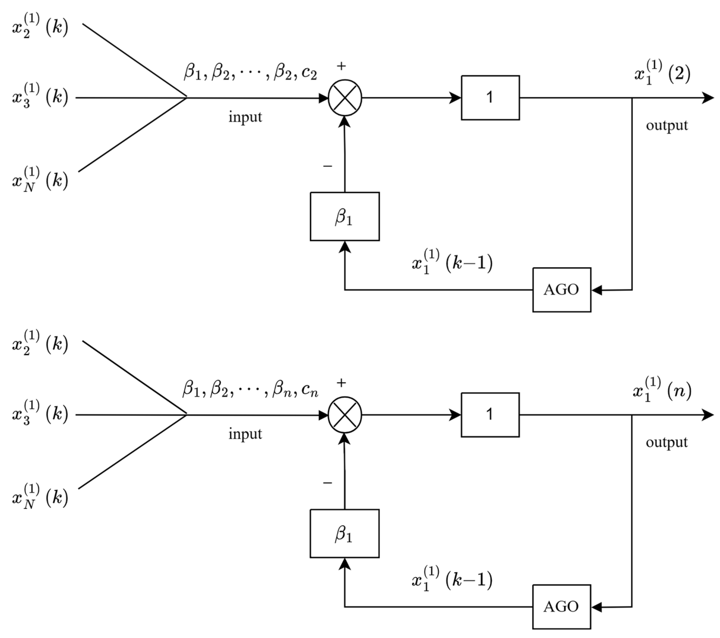
In cybernetics, inputs and outputs have a one-to-one correspondence. At different points in time, the magnitude of the grey action quantity varies. Therefore, $c_2,c_3,\cdots ,$ and $c_n$ are not equal, that is, $c_2\ne c_3\ne \cdots \ne c_n$ [27]. Figure 2 illustrates the relationship between the inputs and outputs of the DGM(1, N) model with different values of $c$. The parameter $c$ in Theorem 1 approximately represents the grey action $c_2,c_3,\cdots ,c_n$, which ignores the differences in the system’s information at different points in time. The results based on Theorem 1 are approximate solutions. Therefore, this paper will fully use the grey action quantity’s information by restoring the grey number format within a known interval.

The grey action quantity’s value may be calculated using formulas for $c_2,c_3,\cdots ,c_n$ based on Equation (1) when $k$ is a different value.

$$\left\{\begin{array}{c}{c}_2=x_1^{\left(1\right)}\left(2\right)-{\beta }_1{x}_1^{\left(1\right)}\left(1\right)-{\sum }_{i=2}^N{\beta }_i{x}_i^{\left(1\right)}\left(2\right)\to k=2\\ c_3=x_1^{\left(1\right)}\left(3\right)-{\beta }_1{x}_1^{\left(1\right)}\left(2\right)-{\sum }_{i=2}^N{\beta }_i{x}_i^{\left(1\right)}\left(3\right)\to k=3\\ ⋮\\ c_n=x_1^{\left(1\right)}\left(n\right)-{\beta }_1{x}_1^{\left(1\right)}\left(n-1\right)-{\sum }_{i=2}^N{\beta }_i{x}_i^{\left(1\right)}\left(n\right)\to k=n\end{array}\right..$$

(8)

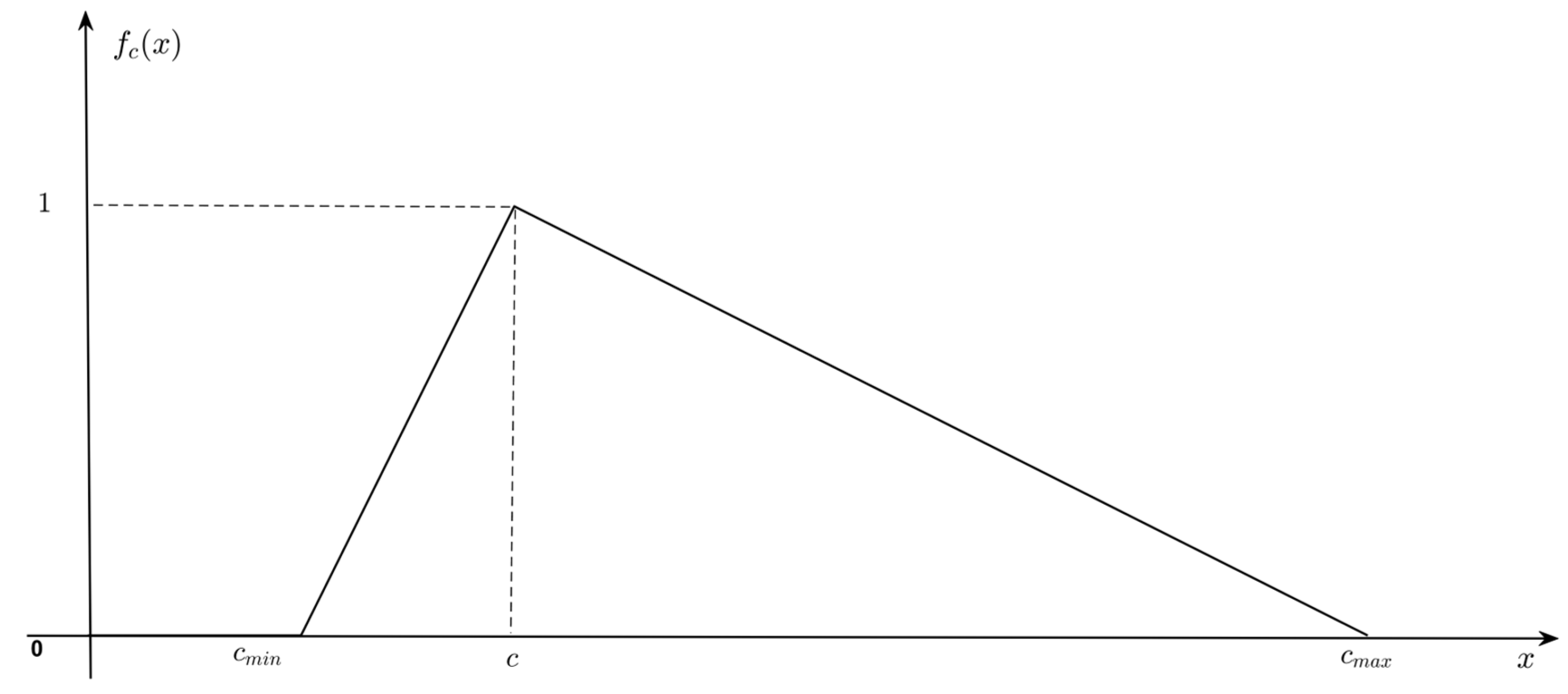
Let $c=\left\{\left.c_2,c_3,\cdots ,c_n\right\}\right.$ be the sequence of the grey action quantities of the DGM(1, N) model. We define $c_{max}$ as the set $c_{max}=\left\{c_2,c_3,\cdots ,c_n\right\}$, and $c_{min}$ as $c_{min}=\left\{c_2,c_3,\cdots ,c_n\right\}$. The grey action quantity, denoted by ${\otimes }_c\in \left[c_{min},c_{max}\right]$, is represented as an interval grey number. The grey system theory employs the function of a possibility degree, which serves to express the probability of a grey number adopting various values within its domain of greyness. Alternatively, it indicates the likelihood of a precise value being the authentic representation of a grey number, symbolized by $f_k\left(x\right)$ [28]. It is probable that the representation of the interval grey number’s “true value,” usually denoted by ${\tilde{\otimes }}_k$, is achieved by fully accounting for the available information. If the interval grey action ${\otimes }_c\in \left[c_{min},c_{max}\right]$ has a larger possible degree function, $f_k\left(x_t\right)$ corresponds to a point $x_t$ within its grey confines. The greater the probability that $x_t$ will be true, the closer $x_t$ is to ${\tilde{\otimes }}_k$. The “kernel” of the interval grey number is the projection point on the X-axis of the center of gravity of the closed geometry formed by its possible degree function [29].

According to the interpretation of the possible degree function [26], Figure 3 displays the possible degree function of ${\otimes }_c\in \left[c_{min},c_{max}\right]$. It is possible to account for the uncertainty of the system inputs and adhere to the grey theory principle of the “non-unique solutions” by using the interval grey action amount.

4. Construction of the DGM(1, N, ${\otimes }_{\mathit{c}}$) Model

4.1. DGM(1, N, ${\otimes }_c$) Model

Definition 2.

Assume the sequences $X_j^{\left(0\right)}, X_j^{\left(1\right)}$ are as defined in Definition 1, ${\beta }_1, {\beta }_i$ are as shown in Theorem 1, ${\otimes }_c\in \left[c_{min},c_{max}\right]$ is the grey action quantity, $P={\left[{\beta }_1,{\beta }_2,\dots ,{\beta }_N,c_{\otimes }\right]}^T$ is the grey number parameter column, denoted

$$x_1^{\left(1\right)}\left(k\right)={\beta }_1{x}_1^{\left(1\right)}\left(k-1\right)+{\sum }_{i=2}^N{\beta }_i{x}_i^{\left(1\right)}\left(k\right)+{\otimes }_c$$

(9)

as the DGM(1, N, ${\otimes }_c$) model with grey action quantities, referred to as the DGM(1, N,  ${\otimes }_c$) model. ${\otimes }_c\in \left[c_{min},c_{max}\right]$ are grey quantities whose the possibility degree function is a triangle with the vertex $c$.

Theorem 3.

Let the sequences $X_j^{\left(0\right)}, X_j^{\left(1\right)},{\beta }_i$, and ${\otimes }_c$ be as shown in Definition 2, then

(1)

Assuming ${\widehat{x}}_1^{\left(1\right)}\left(1\right)=x_1^{\left(0\right)}\left(1\right)$ is the starting value, the DGM(1, N, ${\otimes }_c$) model’s time response equation is

$${\widehat{x}}_{1_{\mathit{min}}}^{\left(1\right)}\left(k\right)={\beta }_1^{k-1}{\widehat{x}}_1^{\left(1\right)}\left(1\right)+{\sum }_{r=2}^k{\beta }_1^{k-r}{\sum }_{i=2}^N{\beta }_i{x}_i^{\left(1\right)}\left(r\right)+\frac{1-{\beta }_1^{k-1}}{1-{\beta }_1}{c}_{min},$$

(10)

$${\widehat{x}}_{1_{mid}}^{\left(1\right)}\left(k\right)={\beta }_1^{k-1}{\widehat{x}}_1^{\left(1\right)}\left(1\right)+{\sum }_{r=2}^k{\beta }_1^{k-r}{\sum }_{i=2}^N{\beta }_i{x}_i^{\left(1\right)}\left(r\right)+\frac{1-{\beta }_1^{k-1}}{1-{\beta }_1}c,$$

(11)

$${\widehat{x}}_{1_{\mathit{max}}}^{\left(1\right)}\left(k\right)={\beta }_1^{k-1}{\widehat{x}}_1^{\left(1\right)}\left(1\right)+{\sum }_{r=2}^k{\beta }_1^{k-r}{\sum }_{i=2}^N{\beta }_i{x}_i^{\left(1\right)}\left(r\right)+\frac{1-{\beta }_1^{k-1}}{1-{\beta }_1}{c}_{max}$$

(12)

(2)

Its cumulative reduction equation is

$$\begin{array}{ll}{\widehat{x}}_{1_{min}}^{\left(0\right)}\left(k\right)& ={\widehat{x}}_1^{\left(1\right)}\left(k\right)-{\widehat{x}}_1^{\left(1\right)}\left(k-1\right)\\ & ={\beta }_1^{k-2}{\widehat{x}}_1^{\left(1\right)}\left({\beta }_1-1\right)+{\displaystyle \sum _{i=2}^N}{\beta }_i{x}_i^{\left(1\right)}\left(k\right)-{\beta }_1^k{c}_{min},k=2,3,\cdots ,n.\end{array}$$

(13)

$${\widehat{x}}_{1_{mid}}^{\left(0\right)}\left(k\right)={\beta }_1^{k-2}{\widehat{x}}_1^{\left(1\right)}\left({\beta }_1-1\right)+\sum _{i=2}^N{\beta }_i{x}_i^{\left(1\right)}\left(k\right)-{\beta }_1^{k}c,k=2,3,\cdots ,n.$$

(14)

$${\widehat{x}}_{1_{max}}^{\left(0\right)}\left(k\right)={\beta }_1^{k-2}{\widehat{x}}_1^{\left(1\right)}\left({\beta }_1-1\right)+\sum _{i=2}^N{\beta }_i{x}_i^{\left(1\right)}\left(k\right)-{\beta }_1^k{c}_{max},k=2,3,\cdots ,n.$$

(15)

The DGM(1, N, ${\otimes }_c$) model extends the DGM(1, N) model, obtained by expanding $c$ from a number to an interval grey number ${\otimes }_c$. This is illustrated by the equation derived from Theorem 3. This model has several characteristics due to the addition of interval grey action quantity, including:

(1)

The structure of the DGM(1, N, ${\otimes }_c$) model incorporates the characteristics of grey numbers. In this model, ${\otimes }_c$ is regarded as an interval grey number with a known possibility function ${\otimes }_c\in \left[c_{min},c_{max}\right]$, thus enabling the uncertainty feature.

(2)

The DGM(1, N, ${\otimes }_c$) model calculation results are interval grey numbers $\otimes \left(k\right)$. Its results are non-unique within an uncertain system, thus satisfying the tenet of the “non-uniqueness of solutions”.

(3)

When the possible degree function for ${\otimes }_c$ has the shape of a triangle, this reduces the grey domain and narrows the range of possible true values. The maximum possible value of ${\otimes }_c$ is ${\tilde{\otimes }}_c=c$, and the largest possible value of the associated interval grey number $\otimes \left(k\right)$ is $\tilde{\otimes }\left(k\right)={\widehat{x}}_{1mid}\left(k\right)$. The simulation results of the DGM(1, N) model are included, demonstrating the DGM(1, N, ${\otimes }_c$) model’s compatibility. The findings of the interval grey number acquired using the DGM(1, N, ${\otimes }_c$) model are judged to be more reliable than the actual numerical values obtained using the traditional model. Therefore, this model can aid decision makers in comprehending the future advancement of the subject.

4.2. Modeling Steps of DGM(1, N, ${\otimes }_c$) Model

The modeling procedures for the DGM(1, N, ${\otimes }_c$) model with grey action quantity are explained below, in conjunction with the modeling and analysis methodology mentioned above.

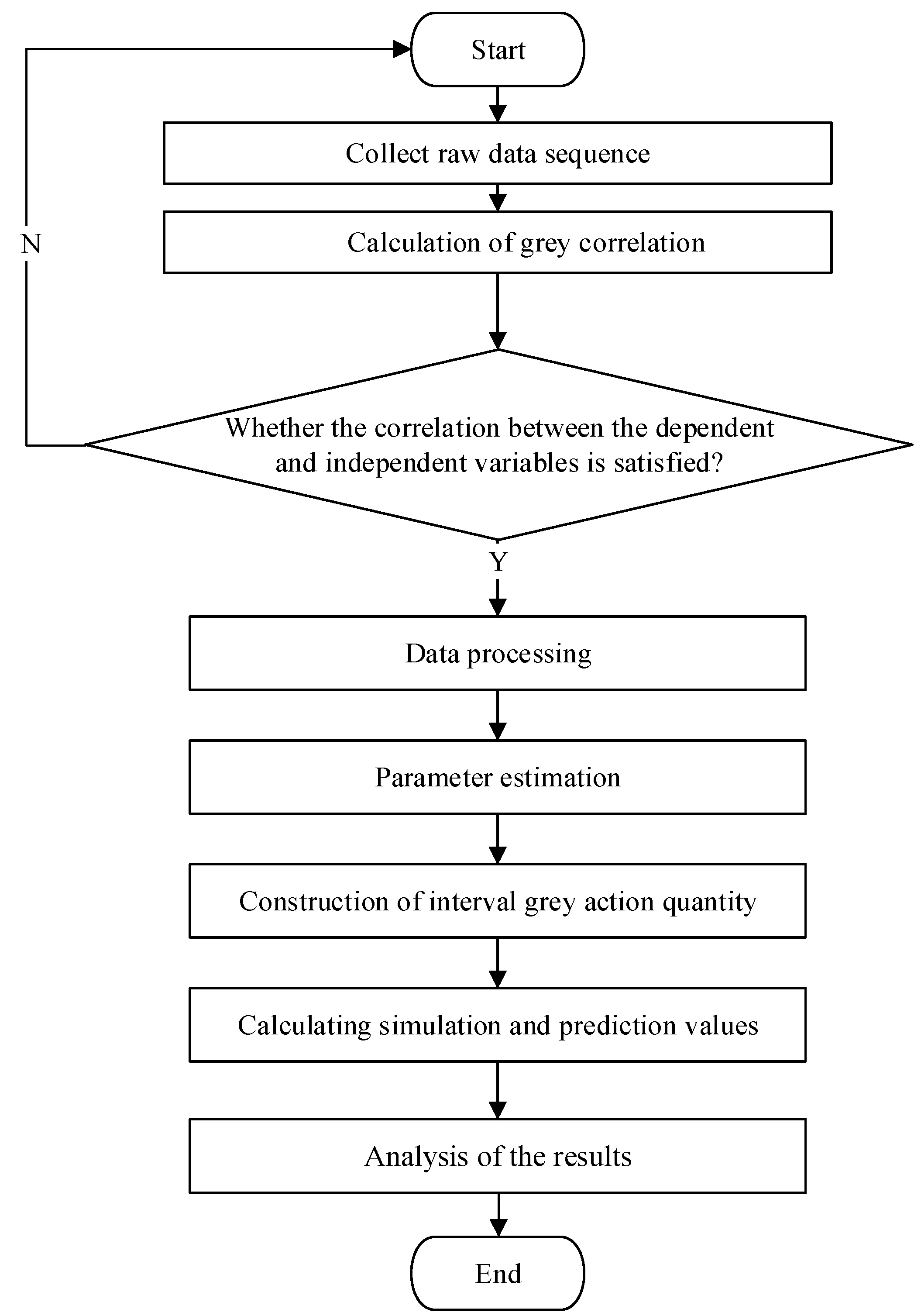
Step 1: The calculation of the grey correlation. Firstly, we calculate the correlation between the dependent and independent variables. Subsequently, taking into consideration the magnitude of the correlation, we ascertain the sequence of independent factors that are strongly correlated.

Step 2: Data processing. The dimensionless processing of the raw data, followed by their first-order cumulative series.

Step 3: Parameter estimation. Using Equation (9), we create the DGM(1, N, ${\otimes }_c$) model and estimate its parameters according to Theorem 1.

Step 4: The construction of the interval grey action quantity. We calculate the model’s parameters according to Theorem 1 and combine them with Equation (8) to obtain a range of values for the interval grey action quantity ${\otimes }_c$.

Step 5: Calculating the simulation and prediction values. Combining the parameter values from Step 4 and Equations (13)–(15) yields the model’s time response equation, which is then simulated and predicted.

Step 6: The analysis of the results. We analyze the reasonableness of the results using the given computations.

In summary, Figure 4 depicts the flowchart for modeling the DGM(1, N, ${\otimes }_c$) model, and the DGM(1, N, ${\otimes }_c$) model’s code is available from the following link: https://github.com/HongtaoRen/GreyPrediction (accessed on 19 June 2023).

5. Numerical Experiment

This study focuses on the total electricity consumption of China as the subject of the numerical validation. The GDP, total population, total energy consumption, and consumption level of residents are selected as the primary factors. The data on the total electricity consumption of China are sourced from the China Electricity Council (https://cec.org.cn/) (accessed on 1 June 2023), while the data on GDP, total population, total energy consumption, and residents’ consumption level are obtained from the China Statistical Yearbook. A grey correlation analysis is utilized to screen the main influencing factors, with the correlation threshold set to 0.6. Based on the results of the correlation calculation, GDP and total energy consumption are identified as independent variables. To better verify the model’s performance, the sample data are divided into two parts in this paper. The first nine years (2010–2018) are used for the model construction, and the last three years (2019–2021) are used for the model prediction. The aforementioned data are used to construct the DGM(1, N, ${\otimes }_c$) model and the calculation results are presented in

Table 1. Actual data and various simulation and prediction values.

$k.$	${\mathit{x}}_1^{\left(0\right)}$	${\widehat{\mathit{x}}}_{1\mathit{m}\mathit{i}\mathit{n}}^{\left(0\right)}$	${\widehat{\mathit{x}}}_{1\mathit{m}\mathit{a}\mathit{x}}^{\left(0\right)}$	${\widehat{\mathit{x}}}_{1\mathit{m}\mathit{i}\mathit{d}}^{\left(0\right)}$
$\mathrm{k}=2$	46,928	46,026.27087	47,839.70479	46,985.47378
$\mathrm{k}=3$	49,591	50,522.05199	49,249.53788	49,848.96475
$\mathrm{k}=4$	53,223	52,169.98529	53,062.92776	52,642.30083
$\mathrm{k}=5$	55,233	55,161.59802	54,535.00674	54,830.16704
$\mathrm{k}=6$	55,500	56,162.90393	56,602.59254	56,395.47408
$\mathrm{k}=7$	59,198	59,404.07514	59,095.53896	59,240.87714
$\mathrm{k}=8$	63,077	63,461.78291	63,678.28743	63,576.30143
$\mathrm{k}=9$	69,163	67,271.10431	67,119.17980	67,190.74493
$\mathrm{k}=10$	72,255	70,163.04833	70,269.65606	70,219.43772
$\mathrm{k}=11$	75,110	71,001.85391	70,269.65606	70,962.28461
$\mathrm{k}=12$	83,128	80,571.45061	80,623.94476	80,599.21704

.

Utilizing the aforementioned calculation outcomes, Figure 5 depicts the distribution of the total electricity consumption of China, along with the associated simulation and prediction data.

The total electricity consumption of China is influenced by various factors, and since the information known in real life cannot uniquely determine the future development of the system, its prediction results should appear nonunique. According to the results of Table 1 and Figure 5, the simulation and prediction results derived from the DGM(1, N, ${\otimes }_c$) model are interval grey numbers, which are consistent with the principle of the “non-uniqueness of solutions” in the context of incomplete information in the grey system theory. The new model’s architecture fulfills the essential characteristics of uncertainty. According to the calculation results of DGM(1, N, ${\otimes }_c$) in Table 1 and Figure 5, the results obtained from the kernel of the interval grey action are the calculation results of the DGM(1, N) model. However, because the new model is an extended model of the DGM(1, N) model, affected by the modeling effect of the DGM(1, N) model, the results of the new model in recent years do not contain actual data, and there are certain errors.

6. Case Study

Previous literature studies [30,31,32,33,34] have identified several factors that influence hydroelectricity consumption, such as economic development level, the scale of hydroelectricity development, demographic factors, and the consumption structure of the population. Considering the accessibility and practicality of the data, this study employs GDP to represent economic development level, total population to represent demographic factors, hydroelectricity production to represent the scale of hydroelectricity, and the consumption level of the population to represent the structure of residential consumption. The data on the hydroelectricity consumption of China and the factors influencing it for 2010–2021 are shown in

Table 2. The hydroelectricity consumption of China and its explanatory variables from 2010 to 2021.

Year	Hydroelectricity Consumption ${\mathit{X}}_1$	GDP $X_2$	Hydroelectricity Production ${\mathit{X}}_3$	Population ${\mathit{X}}_4$	The Consumption Level of the Population ${\mathit{X}}_5$
2010	7.11	412,119.2	711.38	134,091	10,575
2011	6.83	487,940.2	688.05	134,916	12,668
2012	8.52	538,580	862.79	135,922	14,074
2013	8.93	592,963.2	909.61	136,726	15,586
2014	10.34	643,563.1	1059.69	137,646	17,220
2015	10.81	688,858.2	1114.52	138,326	18,857
2016	11.11	746,395.1	1153.27	139,232	20,801
2017	11.16	832,035.9	1165.07	140,011	22,969
2018	11.42	919,281.1	1198.89	140,541	25,245
2019	12.08	986,515.2	1272.54	141,008	27,504
2020	12.50	1,015,986.2	1321.71	141,212	27,438
2021	12.25	1,143,669.7	1300	141,260	31,072

, which were obtained from the China Statistics Yearbook and BP Statistics Review of World Energy. The consumption of hydroelectricity (EJ) is recorded as $X_1$. The GDP (billion yuan), hydroelectricity production (million tons), population (10,000 people), and consumption level of the population are recorded as $X_2$, $X_3$, $X_4$, and $X_5$ in that order. As the difference in magnitude between different indicators can affect the modeling effects of the model, all the data are dimensionless before modeling. A validation process is carried out using a dataset divided into two parts to assess the efficacy of the model in this research. Specifically, the first nine years of data (2010–2018) are utilized to construct the model, and the last three years (2019–2021) are used for the model forecasting.

Step 1: The calculation of the grey correlation. As the strength of each factor’s impact on the main system behavior sequence varies, to avoid redundancy of the influencing factor variables, the degree of correlation between each influencing factor variable and the main system behavior variable was first calculated using a grey correlation analysis before modeling. Moreover, this was used to finally decide the model’s independent variables. A higher grey correlation degree indicates a stronger association between the variables. We chose a correlation threshold of 0.6 to determine the model’s independent variables. Any influencing factor with a correlation degree greater than 0.6 was chosen as an independent variable for the modeling. Let the correlation degree between $X_1$ and the independent variables $X_2, X_3,X_4,\mathrm{and} X_5$ be $\gamma \left(X_1^{\left(0\right)}\left(k\right),X_p^{\left(0\right)}\left(k\right)\right)$. The formula for calculating the grey correlation degree [9] is when $p=2,3,4,5$.

$$\gamma \left(x_1^{\left(0\right)}\left(k\right),x_p^{\left(0\right)}\left(k\right)\right)=\frac{\begin{array}{c}min\\ p\end{array}\begin{array}{c}min\\ k\end{array}\left|x_1^{\left(0\right)}\left(k\right)-x_p^{\left(0\right)}\left(k\right)\right|+\xi \begin{array}{c}max\\ p\end{array}\begin{array}{c}max\\ k\end{array}\left|x_1^{\left(0\right)}\left(k\right)-x_p^{\left(0\right)}\left(k\right)\right|}{\left|x_1^{\left(0\right)}\left(k\right)-x_p^{\left(0\right)}\left(k\right)\right|+\xi \begin{array}{c}max\\ i\end{array}\begin{array}{c}max\\ k\end{array}\left|x_1^{\left(0\right)}\left(k\right)-x_p^{\left(0\right)}\left(k\right)\right|}.$$

(16)

$$\gamma \left(X_1^{\left(0\right)}\left(k\right),X_p^{\left(0\right)}\left(k\right)\right)=\frac{1}{n}{\sum }_{k=1}^n\gamma \left(x_1^{\left(0\right)}\left(k\right),x_p^{\left(0\right)}\left(k\right)\right).$$

(17)

In Equation (16), the resolution factor $\xi$ is usually taken as 0.5. Using Equations (16) and (17), the correlations of the influencing factors were calculated as ${\gamma }_{12}=0.6447$, ${\gamma }_{13}=0.9091$, ${\gamma }_{14}=0.5855, \mathrm{and} {\gamma }_{15}=0.5874.$ $X_2$ and $X_3$ had a strong correlation with $X_1$, and can be classified as strongly correlated factors. Therefore, the variables $X_2$ and $X_3$ were chosen for the modeling.

Step 2: The dimensionless processing of the raw data according to the selected variables to obtain a sequence of characteristic system data and relevant factors. Subsequently,

Table 3. The calculation results of $x_j^{\left(0\right)}\left(k\right)$ after dimensionless processing and $x_j^{\left(1\right)}\left(k\right)$.

$k.$	${\mathit{x}}_1^{\left(0\right)}\left(\mathit{k}\right)$	${\mathit{x}}_2^{\left(0\right)}\left(\mathit{k}\right)$	${\mathit{x}}_3^{\left(0\right)}\left(\mathit{k}\right)$	${\mathit{x}}_1^{\left(1\right)}\left(\mathit{k}\right)$	${\mathit{x}}_2^{\left(1\right)}\left(\mathit{k}\right)$	${\mathit{x}}_3^{\left(1\right)}\left(\mathit{k}\right)$
$\mathrm{k}=1$	1	1	1	1	1	1
$\mathrm{k}=2$	0.96	1.18	0.97	1.96	2.18	1.97
$\mathrm{k}=3$	1.20	1.31	1.21	3.16	3.49	3.18
$\mathrm{k}=4$	1.26	1.44	1.28	4.42	4.93	4.46
$\mathrm{k}=5$	1.45	1.56	1.49	5.87	6.49	5.95
$\mathrm{k}=6$	1.52	1.67	1.57	7.39	8.16	7.52
$\mathrm{k}=7$	1.56	1.81	1.62	8.95	9.97	9.14
$\mathrm{k}=8$	1.57	2.02	1.64	10.52	11.99	10.78
$\mathrm{k}=9$	1.61	2.23	1.69	12.13	14.22	12.47

presents the outcomes of calculating the cumulative sequence of the first order.

Step 3: Solve for the model parameters. Based on Theorem 1, the matrices $B$ and $Y$ may be derived as follows

$$B=\left[\begin{array}{cccc}1& 2.18& 1.97& 1\\ 1.96& 3.49& 3.18& 1\\ 3.16& 4.93& 4.46& 1\\ 4.42& 6.49& 5.95& 1\\ 5.87& 8.16& 7.52& 1\\ 7.39& 9.97& 9.14& 1\\ 8.95& 11.99& 10.78& 1\\ 10.52& 12.22& 12.47& 1\end{array}\right], Y=\left[\begin{array}{c}1.96\\ 3.16\\ 4.42\\ 5.87\\ 7.39\\ 8.95\\ 10.52\\ 12.13\end{array}\right]$$

The parameter column $\widehat{\beta }$ can be obtained from $\widehat{\beta }={\left[{\beta }_1,{\beta }_2,\dots ,c\right]}^T$ as

$$\widehat{\beta }={\left[{\beta }_1,{\beta }_2,\dots ,c\right]}^T={\left(B^{T}B\right)}^{-1}{B}^{T}Y=\left[\begin{array}{c}-0.2094\\ -0.0494\\ 1.2149\\ -0.1115\end{array}\right]$$

Step 4: The construction of the interval grey action volume ${\otimes }_c\in \left[c_{min},c_{max}\right]$. As seen from Definition 1, the data for the development factor ${\beta }_1$ and the driving term factors ${\beta }_i$, $x_i^{\left(0\right)}\left(k\right)$, and $x_i^{\left(1\right)}\left(k\right)$ are known.

According to Equation (8), the amount of grey action $c_k$ at this point $k$ is obtained as

$$\begin{array}{cc}{C}_s& =\left\{\left.c_2,c_3,\cdots ,c_9\right\}\right.\hfill \\ & =\left\{\left.-0.1162,-0.1204,-0.0930,-0.1122,-0.1134,-0.1138,-0.1096,-0.1138\right\}\right.\end{array}$$

Then

$$c_{\mathit{max}}=\mathit{max}\left\{\left.c_2,c_3,\cdots ,c_9\right\}\right.=-0.0930;$$

$$c_{\mathit{min}}=\mathit{min}\left\{\left.c_2,c_3,\cdots ,c_9\right\}\right.=-0.1204.$$

Therefore, the interval grey action quantity ${\otimes }_c\in \left[c_{min},c_{max}\right]$ can be expressed as

$${\otimes }_c\in \left[-0.1204,-0.0930\right], {\tilde{\otimes }}_c=c=-0.1115$$

Step 5: Calculating the simulation and prediction values. Based on Theorem 2 and the vector $P={\left[{\beta }_1,{\beta }_2,\dots ,c_{\otimes }\right]}^T$, when $\mathrm{k}=2,3,4,5,6,7,8,9,10,11,12$ the calculations for ${\widehat{x}}_{1_{min}}^{\left(0\right)}, {\widehat{x}}_{1_{max}}^{\left(0\right)}$ and ${\widehat{x}}_{1_{mid}}^{\left(0\right)}$ are presented in

Table 4. Actual data and various simulation and prediction values.

$k.$	${\mathit{x}}_1^{\left(0\right)}$	${\widehat{\mathit{x}}}_{1\mathit{m}\mathit{i}\mathit{n}}^{\left(0\right)}$	${\widehat{\mathit{x}}}_{1\mathit{m}\mathit{a}\mathit{x}}^{\left(0\right)}$	${\widehat{\mathit{x}}}_{1\mathit{m}\mathit{i}\mathit{d}}^{\left(0\right)}$
$\mathrm{k}=2$	6.83	6.795522	6.9904382	6.858557
$\mathrm{k}=3$	8.52	8.568377	8.5275547	8.555175
$\mathrm{k}=4$	8.93	8.756065	8.7646151	8.758830
$\mathrm{k}=5$	10.34	10.488537	10.486746	10.487958
$\mathrm{k}=6$	10.81	10.778083	10.778458	10.778205
$\mathrm{k}=7$	11.11	11.100164	11.100085	11.100139
$\mathrm{k}=8$	11.16	11.131717	11.131734	11.131723
$\mathrm{k}=9$	11.42	11.483249	11.483246	11.483248
$\mathrm{k}=10$	12.08	12.217202	12.217211	12.217210
$\mathrm{k}=11$	12.50	12.643550	12.64355	12.643551
$\mathrm{k}=12$	12.25	12.182753	12.182755	12.182754

.

Then

$$\begin{array}{l}\otimes \left(2\right)\in \left[6.795522,6.9904382\right],{\widehat{x}}_1^{\left(0\right)}\left(2\right)=\tilde{\otimes }\left(2\right)=6.858557;\\ \otimes \left(3\right)\in \left[8.5275547,8.568377\right],{\widehat{x}}_1^{\left(0\right)}\left(3\right)=\tilde{\otimes }\left(3\right)=8.758830;\\ \otimes \left(4\right)\in \left[8.756065,8.7646151\right],{\widehat{x}}_1^{\left(0\right)}\left(4\right)=\tilde{\otimes }\left(4\right)=8.758830;\\ \otimes \left(5\right)\in \left[10.486746,10.488537\right],{\widehat{x}}_1^{\left(0\right)}\left(5\right)=\tilde{\otimes }\left(5\right)=10.487958;\\ \otimes \left(6\right)\in \left[10.778083,10.778458\right],{\widehat{x}}_1^{\left(0\right)}\left(6\right)=\tilde{\otimes }\left(6\right)=10.778205;\\ \otimes \left(7\right)\in \left[11.100085,11.100164\right],{\widehat{x}}_1^{\left(0\right)}\left(7\right)=\tilde{\otimes }\left(7\right)=11.100139;\\ \otimes \left(8\right)\in \left[11.131717,11.131734\right],{\widehat{x}}_1^{\left(0\right)}\left(8\right)=\tilde{\otimes }\left(8\right)=11.131723;\\ \otimes \left(9\right)\in \left[11.483246,11.483249\right],{\widehat{x}}_1^{\left(0\right)}\left(9\right)=\tilde{\otimes }\left(9\right)=11.483248;\\ \otimes \left(10\right)\in \left[12.217202,12.217211\right],{\widehat{x}}_1^{\left(0\right)}\left(10\right)=\tilde{\otimes }\left(10\right)=12.217210;\\ \otimes \left(11\right)\in \left[12.643550,12.64355\right],{\widehat{x}}_1^{\left(0\right)}\left(10\right)=\tilde{\otimes }\left(10\right)=12.643551;\\ \otimes \left(12\right)\in \left[12.182753,12.182755\right],{\widehat{x}}_1^{\left(0\right)}\left(11\right)=\tilde{\otimes }\left(11\right)=12.182754\end{array}$$

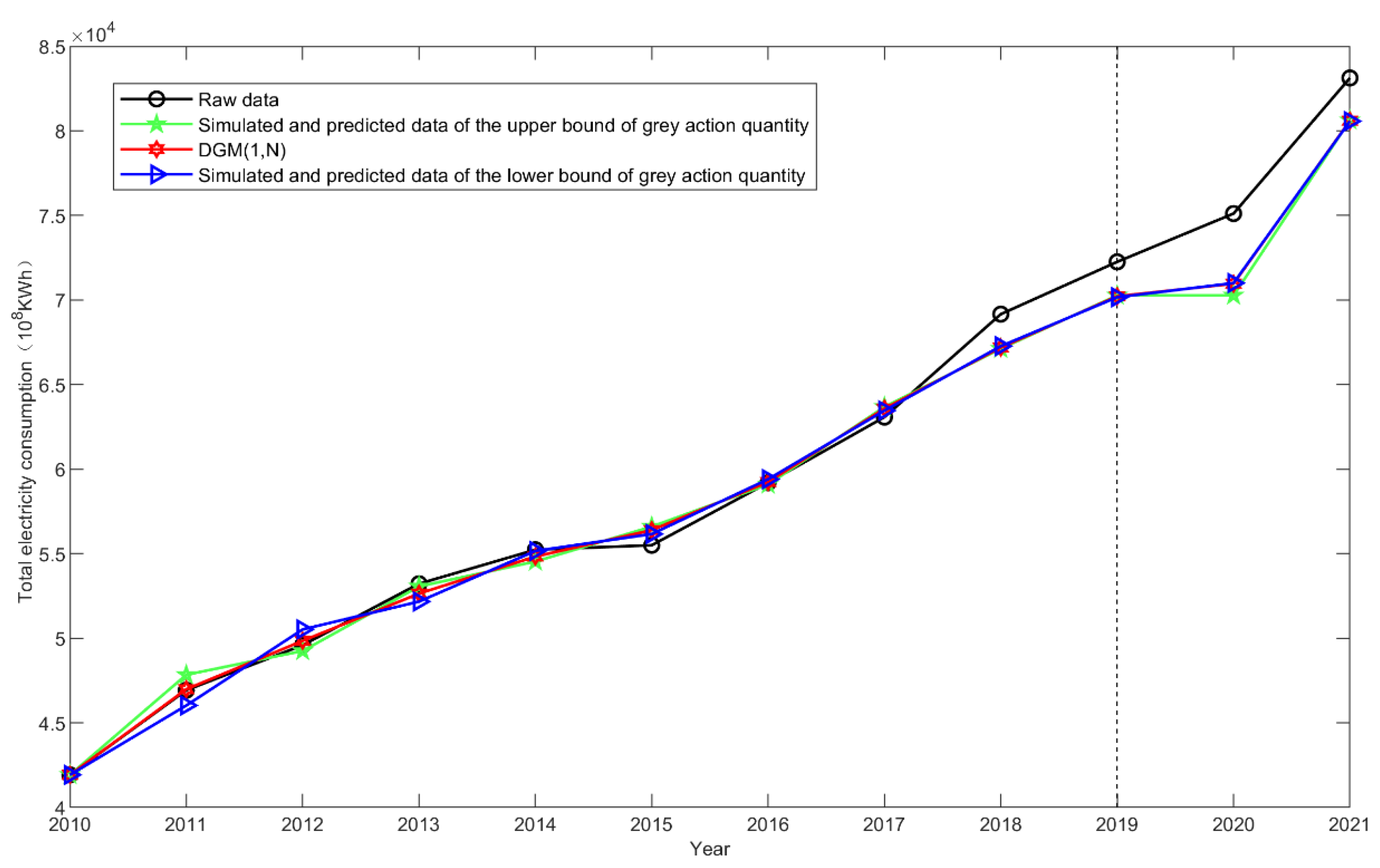
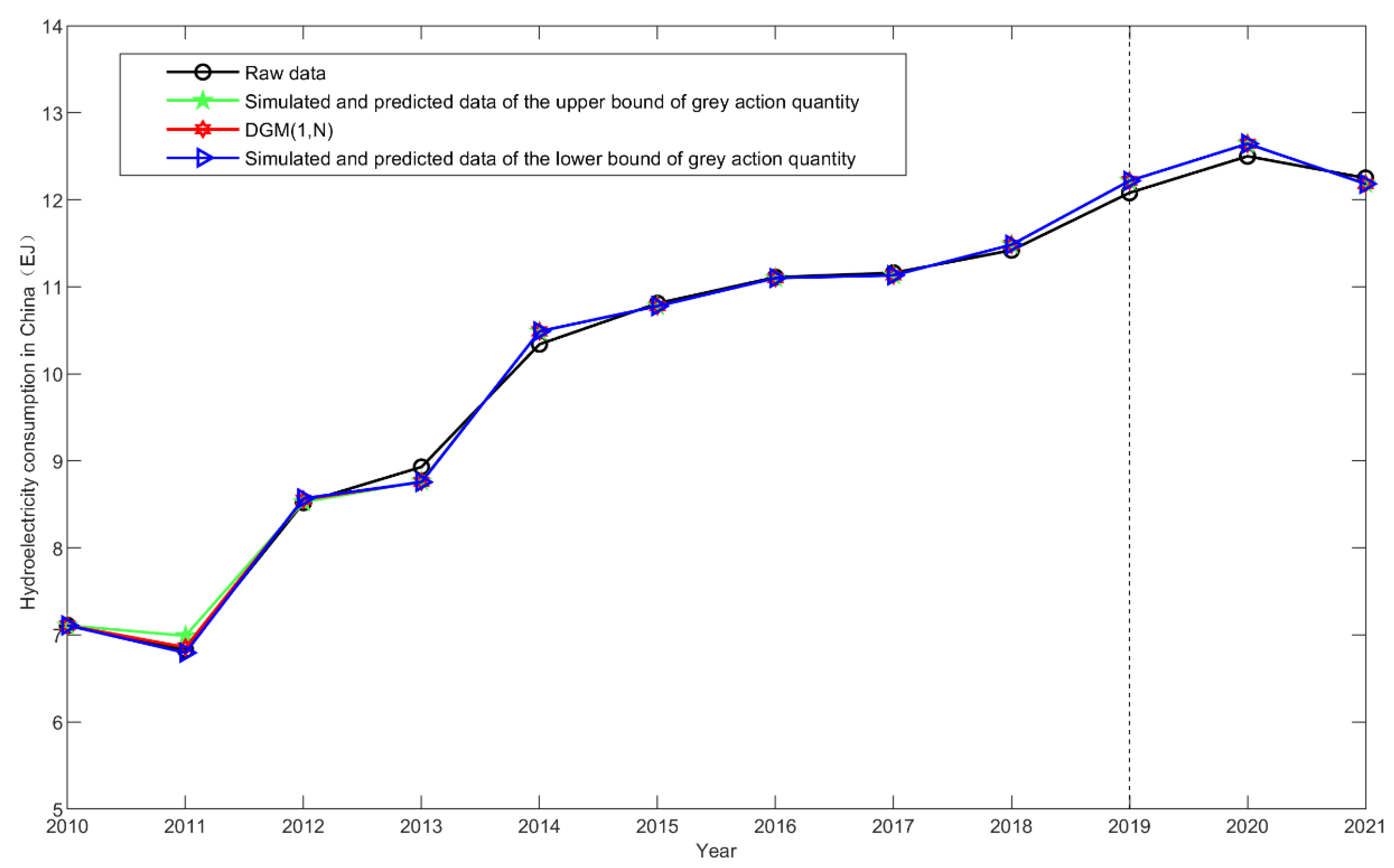
Step 6: The analysis of the rationality of the results. Figure 6 displays the raw data along with the various simulated and predicted data, based on the calculations presented above. Before illustrating the model’s reasonableness as demonstrated in this paper, an analysis of the inadequacies associated with the DGM(1, N) model for simulating the hydroelectricity consumption of China was performed.

The parameter $c$ signifies the combined impact of numerous intricate and uncertain factors in the traditional DGM(1, N) model, thereby rendering it intrinsically uncertain and necessitating its representation as a grey number. Nonetheless, when applying the DGM(1, N) model to a specific system, parameter $c$ is determined through the least squares method, resulting in a unique numerical value. This approach neglects the grey number action quantity’s uncertainty characteristics, resulting in a less reliable simulation. As a grey prediction model, the DGM(1, N) model operates with incomplete information and reveals the complexity and variability of a system’s influencing factors. The grey system theory’s principle of the “non-uniqueness of solutions” indicates that solutions for incomplete information and uncertainty are not unique. Consequently, the DGM(1, N) model’s simulation and prediction results should also be non-unique [27].

This paper calculates and compares grey action quantities at distinct time points to obtain the representation of the interval grey action amount $c$ [25]. A model known as DGM(1, N, ${\otimes }_c$) is constructed, taking into consideration the aforementioned information. The aforementioned model enhances the DGM(1, N) model’s rationality through the means below.

(1)

The proposed model’s architecture fulfills the critical features of uncertainty that are typically associated with grey prediction models. In this model, the grey action amount is represented by an interval grey number that has a foregone possibility function. The model introduces the notion of interval grey action, facilitating the restitution of the interval grey number form of $c$ in situations where the information is incomplete. Furthermore, it also achieves a compartmentalized structure distinct from the DGM(1, N) model.

(2)

The proposed model’s simulation and prediction outcomes satisfy the “non-uniqueness of solutions” principle. This model produces a sequence of interval grey numbers instead of a singular numerical outcome, which distinguishes it from the conventional DGM(1, N) model.

(3)

The proposed model is consistent with the “least information” tenet of the grey systems theory. This model can effectively utilize the information on grey quantities at various time points. In contrast, the conventional model estimates the grey effect using the least squares approach, which ends up as an actual number, a simplification that results in the omission of important information.

(4)

The outcome obtained through the DGM(1, N, ${\otimes }_c$) model provides more informative results. Specifically, the DGM(1, N, ${\otimes }_c$) model prediction structure takes the form of intervals, which can offer decision makers a clearer understanding of the range of variation in the system. In contrast, the traditional DGM(1, N) model relies on a deterministic real number as its forecast result, which tends to make decision makers doubt its reliability. Thus, having a definite interval rather than a definite number can enhance the informativeness of the prediction, making it easier for decision makers to assess a system’s behavior and make informed decisions.

(5)

The proposed model extends the DGM(1, N) model, which is compatible with it. Specifically, when ${\tilde{\otimes }}_c=c$ in the DGM(1, N, ${\otimes }_c$) model, the calculation results are ${\widehat{x}}_{1_{mid}}\left(k\right)$. The aforementioned outcome is consistent with the conventional DGM(1, N) model’s simulated and predicted findings. Thus, we can conclude that the DGM(1, N, ${\otimes }_c$) model is compatible with the DGM(1, N) model. However, as can be seen from the results in Figure 6, due to the modeling effect of the DGM(1, N) model, the new model has had some errors in terms of simulation and prediction in recent years and does not contain actual data, which is also the limitation of the model in this paper.

Based on the above results, China’s hydroelectricity consumption shows an overall increasing trend, but there is a noticeable fluctuation in its hydroelectricity consumption during the forecasting period. Therefore, the government should adopt reasonable energy price regulation measures. Dynamic adjustments in energy prices can help to guide consumers to make rational use of their energy, while providing a stable operating environment for energy enterprises.

According to the forecast results for 2021, China’s hydroelectricity consumption demonstrates a declining trend. To further achieve the goal of low-carbon development, the government could implement policies to promote the development and utilization of renewable energy sources, such as solar and wind energy, as well as support the research and application of new clean energy technologies. These measures will facilitate the optimization of the energy structure and promote the development of an environmentally friendly economy.

When forecasting hydroelectricity consumption, this study primarily considered the influence of domestic gross domestic product (GDP) and hydroelectricity production. In 2021, domestic GDP shows an upward trend, but hydroelectricity consumption, on the other hand, experiences a decline, possibly due to a decrease in hydroelectric production. This pattern was also evident in 2011, further validating the close correlation between hydroelectricity consumption and hydroelectric production. Hence, the country should intensify its efforts towards developing and utilizing hydroelectric resources to promote the growth of clean energy. Given that hydroelectricity consumption is influenced by multiple factors, leading to interval-based forecasting results, the government should establish an emergency energy reserve mechanism to ensure sufficient energy reserves during unforeseen circumstances.

7. Conclusions

This study addressed the problem of the traditional DGM(1, N) model’s prediction results, which do not account for the “non-uniqueness of solutions” principle in the grey system theory.

We converted the DGM(1, N) model’s grey action quantity back into an interval grey action quantity by adding it. Subsequently, we established a DGM(1, N, ${\otimes }_c$) model, which includes the interval grey action quantity. The proposed model has several advantages, including the grey prediction uncertainty feature due to the characteristics of the grey numbers present in its structure. Additionally, the DGM(1, N, ${\otimes }_c$) model’s simulation and prediction outcomes are interval grey numbers, satisfying the “non-uniqueness of solutions” principle. To verify the model’s reasonableness, we forecasted the hydroelectricity consumption of China using the DGM(1, N, ${\otimes }_c$) model. The results demonstrated a higher level of reasonableness in the simulation and prediction results. Finally, based on the research results, it was proposed that the government should regulate energy prices, increase the development and utilization of hydropower, expand its investment in renewable energy, and establish emergency energy reserves to promote the achievement of low-carbon goals. Although this paper simply expanded the $c$ to an interval grey number ${\otimes }_c\in \left[c_{min},c_{max}\right]$, the proposed DGM(1, N, ${\otimes }_c$) model made it a true grey attribute.

However, the model still has the defect of not including all the actual values in the process of its modeling. To further enhance the modeling effectiveness and rationality of grey forecasting models, we will use DGM(1, N, ${\otimes }_c$) as the foundation of our study and explore the grey attributes of other grey prediction models in greater depth in future research.

References

- Li, C.; Cao, Y.; Zhang, M.; Wang, J.; Liu, J.; Shi, H.; Geng, Y. Hidden Benefits of Electric Vehicles for Addressing Climate Change. Sci. Rep. 2015, 5, 9213. [Google Scholar] [CrossRef] [PubMed] [Green Version]
- He, X.; Wang, Y.; Zhang, Y.; Ma, X.; Wu, W.; Zhang, L. A novel structure adaptive new information priority discrete grey prediction model and its application in renewable energy generation forecasting. Appl. Energy 2022, 325, 119854. [Google Scholar] [CrossRef]
- Jamil, R. Hydroelectricity consumption forecast for Pakistan using ARIMA modeling and supply-demand analysis for the year 2030. Renew. Energy 2020, 154, 1–10. [Google Scholar] [CrossRef]
- De Cabral, J.; Legey, L.F.L.; de Cabral, M.V. Electricity consumption forecasting in Brazil: A spatial econometrics approach. Energy 2017, 126, 124–131. [Google Scholar] [CrossRef]
- Tang, L.; Wang, X.; Wang, X.; Shao, C.; Liu, S.; Tian, S. Long-term electricity consumption forecasting based on expert prediction and fuzzy Bayesian theory. Energy 2018, 167, 1144–1154. [Google Scholar] [CrossRef]
- De Felice, M.; Alessandri, A.; Catalano, F. Seasonal climate forecasts for medium-term electricity demand forecasting. Appl. Energy 2015, 137, 435–444. [Google Scholar] [CrossRef]
- Ruiz, L.; Rueda, R.; Cuéllar, M.; Pegalajar, M. Energy consumption forecasting based on Elman neural networks with evolutive optimization. Expert Syst. Appl. 2018, 92, 380–389. [Google Scholar] [CrossRef]
- Shine, P.; Scully, T.; Upton, J. Murphy Annual electricity consumption prediction and future expansion analysis on dairy farms using a support vector machine. Appl. Energy 2019, 250, 1110–1119. [Google Scholar] [CrossRef]
- Liu, S.F. Grey Systems: Theory and Applications; Science Press: Beijing, China, 2017. [Google Scholar]
- Şahin, U.; Ballı, S.; Chen, Y. Forecasting seasonal electricity generation in European countries under Covid-19-induced lockdown using fractional grey prediction models and machine learning methods. Appl. Energy 2021, 302, 117540. [Google Scholar] [CrossRef]
- Xie, N.-M.; Liu, S.-F. Discrete grey forecasting model and its optimization. Appl. Math. Model. 2009, 33, 1173–1186. [Google Scholar] [CrossRef]
- Ding, S. A novel discrete grey multivariable model and its application in forecasting the output value of China’s high-tech industries. Comput. Ind. Eng. 2019, 127, 749–760. [Google Scholar] [CrossRef]
- Tu, L.; Chen, Y. An unequal adjacent grey forecasting air pollution urban model. Appl. Math. Model. 2021, 99, 260–275. [Google Scholar] [CrossRef]
- Zhang, K. Multivariate discrete grey model base on dummy drivers. Grey Syst. Theory Appl. 2016, 6, 246–258. [Google Scholar] [CrossRef]
- Dang, Y.G.; Wei, L.; Ding, S. Delay multi-variables discrete grey model based on the driving-information control and its application. Control. Decis. 2017, 32, 1672–1680. [Google Scholar]
- Zhang, K.; Qu, P.P.; Zhang, Y.T. Delay multi-variables discrete grey model and its application. Syst. Eng.-Theory Pract. 2015, 35, 2092–2103. [Google Scholar]
- Ye, L.; Xie, N.; Hu, A. A novel time-delay multivariate grey model for impact analysis of CO2 emissions from China’s transportation sectors. Appl. Math. Model. 2020, 91, 493–507. [Google Scholar] [CrossRef]
- Ding, S.; Dang, Y.G.; Xu, N.; Wang, J.J.; Geng, S.S. Construction and optimization of a multi-variables discrete grey power model. Syst. Eng. Electron. 2018, 40, 1302–1309. [Google Scholar]
- Ding, S.; Xu, N.; Ye, J.; Zhou, W.; Zhang, X. Estimating Chinese energy-related CO2 emissions by employing a novel discrete grey prediction model. J. Clean. Prod. 2020, 259, 120793. [Google Scholar] [CrossRef]
- Luo, D.; An, Y.M.; Wang, X.L. Time-delayed accumulative TDAGM (1,N,t) model and its application in grain production. Control. Decis. 2021, 36, 2002–2012. [Google Scholar]
- Ye, L.L.; Xie, N.M.; Luo, D. Construction and application of cumulative time-lag nonlinear ATNDGM(1,N) model. Syst. Eng.-Theory Pract. 2021, 41, 2414–2427. [Google Scholar]
- Ma, X.; Xie, M.; Wu, W.; Zeng, B.; Wang, Y.; Wu, X. The novel fractional discrete multivariate grey system model and its applications. Appl. Math. Model. 2019, 70, 402–424. [Google Scholar] [CrossRef]
- Zhang, X.; Dang, Y.; Ding, S.; Wang, J. A novel discrete multivariable grey model with spatial proximity effects for economic output forecast. Appl. Math. Model. 2023, 115, 431–452. [Google Scholar] [CrossRef]
- Zeng, B.; Duan, H.; Bai, Y.; Meng, W. Forecasting the output of shale gas in China using an unbiased grey model and weakening buffer operator. Energy 2018, 151, 238–249. [Google Scholar] [CrossRef]
- Li, S.L.; Gong, K.; Zeng, B.; Zhou, W.H.; Zhang, Z.Y.; Li, A.X.; Zhang, L. Development of the GM(1,1,⊗b) model with a trapezoidal possibility function and its application. Grey Syst. Theory Appl. 2022, 12, 339–356. [Google Scholar] [CrossRef]
- Deng, J.L. Grey Theory Basis; Huazhong University of Science and Technology Press of China: Wuhan, China, 2002. [Google Scholar]
- Zeng, B.; Gou, X.Y.; Zhang, Z.W. Research on the non-uniqueness of solutions of the mean difference GM(1,1) model based on interval grey interaction. Chin. J. Manag. Sci. 2022, 30, 247–255. [Google Scholar]
- Zeng, B.; Li, S.L.; Meng, W. Grey Prediction Theory and Its Application; Science Press: Beijing, China, 2020. [Google Scholar]
- Xiong, P.; He, Z.; Chen, S.; Peng, M. A novel GM(1,N) model based on interval gray number and its application to research on smog pollution. Kybernetes 2019, 49, 753–778. [Google Scholar] [CrossRef]
- Zheng, C.; Wu, W.-Z.; Xie, W.; Li, Q.; Zhang, T. Forecasting the hydroelectricity consumption of China by using a novel unbiased nonlinear grey Bernoulli model. J. Clean. Prod. 2020, 278, 123903. [Google Scholar] [CrossRef]
- Duan, H.; Luo, X. A novel multivariable grey prediction model and its application in forecasting coal consumption. ISA Trans. 2022, 120, 110–127. [Google Scholar] [CrossRef]
- Wu, L.; Gao, X.; Xiao, Y.; Yang, Y.; Chen, X. Using a novel multi-variable grey model to forecast the electricity consumption of Shandong Province in China. Energy 2018, 157, 327–335. [Google Scholar] [CrossRef]
- Liu, Y.; Yang, Y.; Pan, F.; Xue, D. A conformable fractional unbiased grey model with a flexible structure and it’s application in hydroelectricity consumption prediction. J. Clean. Prod. 2022, 367, 133029. [Google Scholar] [CrossRef]
- Ding, Y.; Dang, Y. Forecasting renewable energy generation with a novel flexible nonlinear multivariable discrete grey prediction model. Energy 2023, 277, 127664. [Google Scholar] [CrossRef]
Figure 1.
The DGM(1, N) model’s structural diagram.
Figure 2.
Input and output correspondence for the DGM(1, N) model.
Figure 3.
Possibility degree function of interval grey action quantity.
Figure 4.
Flowchart of DGM(1, N, ) model.
Figure 5.
Total electricity consumption and related simulation and prediction data.
Figure 6.
Comparisons of raw data with simulation and prediction data.