AatMatch: Adaptive Adversarial Training in Semi-Supervised Learning Based on Data-Driven Decision-Making Models

Abstract

Data-driven decision-making is the process of using data to inform your decision-making process and validate a course of action before committing to it. The quality of unlabeled data in real-world scenarios presents challenges for semi-supervised learning. Effectively leveraging unlabeled data for learning is challenging due to the need for labeled information, while the scarcity of labeled data requires efficient and flexible data augmentation methods. To address these challenges, this paper proposes the AatMatch algorithm, which uses a momentum model, coarse learning, and adversarial training to generate adversarial examples for different classes. The algorithm sets the threshold for generating pseudo-labels and reinforces the results with adversarial perturbations based on evaluation results. In addition, a more refined learning strategy for unlabeled data is adjusted by setting adaptive weights based on the confidence of each unlabeled data point, thereby mitigating the adverse effects of low-confidence unlabeled data on the model. Experimental evaluations on several datasets, including CIFAR-10, CIFAR-100, and SVHN, demonstrate the effectiveness of the proposed AatMatch algorithm in semi-supervised learning. Specifically, the algorithm achieves the lowest error rates for multiple scenarios on these datasets.

1. Introduction

In deep learning [1], the quantity and quality of training data are critical to the performance of a model. However, obtaining large-scale yet fully annotated datasets in real-life situations is impractical due to the enormous human and financial resources required for their preparation [2]. Moreover, in specialized fields such as medical imaging [3], accurate labelling requires experienced experts, making acquiring labeled datasets even more challenging. Therefore, reducing the demand for models on data quality and quantity while improving model performance has become an important research issue. In the era of big data, data annotation costs are high, and obtaining labeled data takes a long time, limiting the application of deep learning algorithms. Semi-supervised learning can use fewer labeled data and improve model performance through the information in unlabeled data. Such methods save costs and improve the model’s efficiency and accuracy [4]. Thus, semi-supervised learning is widely significant in practical applications.

Deep semi-supervised learning methods are currently divided into pseudo-labelling [5] and consistency regularization [6]. The critical element of the consistency regularization methods is data augmentation, and most consistency regularization methods adapt RandAugment [7]. However, such random augmentation methods at the image level lack specificity for the model. Therefore, this paper proposes a new data augmentation method that combines curriculum learning [8] and adversarial training [9] together. This method can add targeted perturbations to the model’s gradient direction based on the learning effect of the class. The generated adversarial samples can be as far away from the original samples as possible without crossing the classification boundary, making the model’s classification boundary in the low-density area more robust.

In the semi-supervised learning scenario, only a small amount of labeled data is available, and it is not possible to use an additional validation set to determine the model’s performance on different classes. However, there is a large amount of unlabeled data available. Therefore, we analyze the characteristics of this data and use the obtained results to assist in setting a more reasonable learning strategy for the model, which is referred to as ‘Data-Driven Decision-Making’. In general, we can use the historical information of unlabeled data to determine the learning effect of the model. However, this leads to the problem of parameter inconsistency in the model. To solve this problem, this paper proposes using a new model to evaluate the learning effect of classes and adopting a momentum model to reduce training computation. Based on the evaluation results, different adversarial perturbation strengths, adversarial sample generation thresholds, and pseudo-label generation thresholds are set. When introducing adaptive thresholds, more low-confidence samples participate in the training. To reduce the negative impact of low-confidence false labels, we set adaptive weights for unlabeled data and adjust the impact of unlabeled data on the model in a more fine-grained manner. Therefore, the algorithm proposed in this paper is called AatMatch. Our contributions are four-fold:

• Firstly, we propose a novel momentum update model specifically designed to evaluate the learning effect of each class. The traditional approach of using historical information in semi-supervised learning may lead to serious consistency problems. However, incorporating an additional model can address this issue without compromising the training process.
• Secondly, we introduce an adaptive adversarial training method that leverages course learning to generate targeted data augmentations. Specifically, we propose a new data augmentation approach that adds targeted perturbations in the gradient direction of each class based on its learning effect. This approach generates adversarial examples that are both effective and efficient in improving model performance.
• Thirdly, we propose a weight-setting mechanism that assigns weights to each unlabeled data sample based on its confidence level, effectively reducing the negative impact of low-confidence pseudo-labelling on the model.
• Lastly, we validate the effectiveness of our proposed AatMatch algorithm on several different datasets. Our experiments demonstrate that the proposed approach achieves state-of-the-art performance on CIFAR10, CIFAR100, and SVHN datasets. The results showcase the potential of our approach to overcome the challenge of limited labeled data and demonstrate its potential for practical applications in the real world.

2. Related Work

The consistency regularization method improves the generalization performance of a model by reducing the difference in data prediction before and after perturbation. Laine et al. [10] proposed the $\mathsf{\Pi }$ model and temporal ensembling model, in which the same unlabeled data are input into the network twice during training. After such different enhancements and dropouts, the outputs are subject to consistency regularization constraints. The temporal ensembling model imposes consistent regularization constraints on the current model prediction results and the Exponential Moving Average (EMA) weights results. Miyato et al. [11] proposed the Virtual Adversarial Training (VAT) model to enhance the robustness and generalization of the model by introducing adversarial training to semi-supervised learning. They achieve this by adding adversarial noise to unlabeled data and then imposing consistent regularization on the original output of the model and the output after adding adversarial noise to improve prediction accuracy. Tarvainen et al. [12] proposed the Mean Teacher model, which is divided into the teacher model and the student model. In each update step, the teacher model is updated based on the EMA weights of the student model, effectively solving the updating problem in the temporal ensembling model. Verma et al. [13] proposed the Interpolation Consistency Training (ICT) algorithm, which applies the mixup [14] technique to unlabeled data and trains by restricting the prediction of the mixup data to the mixup predicted by the data, with the advantage that it is simple and computationally small and does not require large computational power such as VAT. Xie et al. [15] proposed a semi-supervised learning algorithm UDA using the latest data enhancement and proposed a Training Signal Annealing (TSA) method.

Pseudo-labelling refers to using a specific method to label data without labels. The usual method is to select the model prediction probability that exceeds the threshold as pseudo-labels. Lee et al. [5] explained how pseudo-labels work. Rizve et al. [16] proposed the UPS algorithm, which introduces the idea of negative sampling and the double standard of uncertainty and probability threshold to screen pseudo-labels. This method improves the accuracy of pseudo-labels and reduces false pseudo-labels. Wang et al. [17] proposed using a pseudo-label group comparison mechanism to reduce the impact of noisy labels. The above methods enhance pseudo-labels’ confidence by different processing methods for unlabeled data and achieve good experimental results, but they do not consider labeled data.

Many researchers combine labelling methods with consistency regularization methods or other algorithms. Berthelot et al. [18] proposed MixMatch, which enhances each unlabeled sample K times and averages the predictions of different enhancements to reduce entropy. The predicted probability distribution is then sharpened before providing the final pseudo-label, and mixup regularization is applied to both labeled and unlabeled data. Berthelot et al. [19] proposed the ReMixMatch, by aligning the labeled predictions of unlabeled data using the label distribution of labeled data and using the predictions of weakly augmented samples as the training target for strongly augmented samples. Sohn et al. [20] proposed the FixMatch. FixMatch simplifies consistency regularization and pseudo-labelling by using both weakly and strongly enhanced methods to obtain two images for each unlabeled image. The prediction results of the weakly enhanced image are used as a class of pseudo-labeled, and the cross-entropy between the predictions of the strongly enhanced images is trained as a loss using a fixed threshold. Li et al. [21] proposed the CoMatch, which combines the idea of graph and contrast learning with semi-supervised learning to utilize the principle of graph structure consistency between the image probabilities predicted by weak data enhancement and the embedding features of images enhanced by strong data. Zhang et al. [22] proposed the FlexMatch algorithm using dynamic thresholds by category, while Yang et al. [23] proposed class-aware contrastive semi-supervised learning (CCSSL), which divides unlabeled data into reliable in-distribution and out-distribution data with noise and uses feature clustering and contrast learning approaches to enhance the model’s ability to fuse downstream tasks. Zheng et al. [24] proposed SimMatch to enhance the learning ability of the model for features using self-supervised learning to generate pseudo-labels with higher confidence by interacting semantic similarity and instance similarity.

In summary, various methods have been proposed to tackle the challenges of semi-supervised learning. The field continues to advance rapidly with the development of new techniques and the integration of multiple approaches.

3. Methodology

3.1. Momentum Model and Adaptive Adversarial Training

For an C-class classification problem, let us define $X=\{(\overrightarrow{x_b},y_b);b\in (1,\dots ,B)\}$ be a batch of $B$ labeled examples, where $\overrightarrow{x_b}$ is the training example, $y_b$ is the label corresponding to $\overrightarrow{x_b}$. Let $U=\{(\overrightarrow{u_b});b\in (1,\dots ,,\mu B)\}$ be a batch of $\mu B$ unlabeled examples where $\mu$ is a hyperparameter that determines the relative sizes of $X$ and $U$.

In this section, we detail how our algorithm solves the parameter consistency problem of the model and reduces the interference of erroneous pseudo labels on model learning. The method leverages two augmentations: “weak” and “strong”. Weak augmentation $\alpha \left(\right)$ is a standard flip-and-shift augmentation strategy. In contrast, strong augmentation $A\left(\right)$ adopts RandAugment [7], making the augmentation image produce severe distortion and cause a certain degree of distortion.

Semi-supervised learning is a challenging task where only a limited amount of labeled data is available. If a portion of the labeled data is then separated from the training set as the validation set, this will result in less labeled data being used for learning and worse model performance. To mitigate this problem, several approaches leverage the model’s prediction information from previous iterations to assist in training. However, incorporating historical information can cause model inconsistency. We propose a momentum model that utilizes historical information to address this issue while reducing the consistency problem. The momentum model does not require additional training. Its parameters can be obtained through Exponential Moving Average (EMA) updates based on the parameters of the primary model, as shown in Equation (1), where $m \in \left[\mathrm{0,1}\right)$ is a momentum coefficient, ${\theta }^{\prime }$ is a parameter of the momentum model, and $\theta$ is a parameter of the classification model.

$${\theta }^{\prime }=\left(1-m\right)\theta +m{\theta }^{\prime }$$

(1)

The consistency of prediction results for each mini-batch can be effectively improved by a slowly updating model. Then, the class learning effect ${\sigma }_t\left(c\right)$ corresponding to class $c,\mathrm{w}\mathrm{h}\mathrm{e}\mathrm{r}\mathrm{e} c=1,\dots ,C$, is judged based on the output of the momentum model:

$${\sigma }_t\left(c\right)={\sum }_{n=1}^N𝟙\left(\mathit{max}\left(p_{{\theta }^{\prime }}^t\left(y∣\alpha \left(\overrightarrow{u_b}\right)\right)\right)>\tau \right)\cdot 𝟙\left(q_{{\theta }^{\prime }}^t\left(\alpha \left(\overrightarrow{u_b}\right)\right)=c\right)$$

(2)

where $q_{{\theta }^{\prime }}^t\left(\alpha \left(\overrightarrow{u_b}\right)\right)=argmax\left(p_{{\theta }^{\prime }}^t\left(y∣\alpha \left(\overrightarrow{u_b}\right)\right)\right)$ is the pseudo label for unlabeled data $\overrightarrow{u_b}$ at epoch/time step $t$, $N$ is the total number of unlabeled data, $p_{{\theta }^{\prime }}^t\left(y∣\alpha \left(\overrightarrow{u_b}\right)\right)$ is the model’s prediction for unlabeled data $\overrightarrow{u_b}$ at epoch/time step $t$, and $𝟙\left(\right)$ means 1 if the condition in the brackets is met, otherwise it is 0. Following the FlexMatch approach, we proceed to normalize ${\mathsf{\sigma }}_t\left(c\right)$. Subsequently, we employ flexible adjustments to the threshold for the pseudo-label of the class, represented by ${\mathcal{T}}_t\left(c\right)$, and the strength of the adversarial perturbation, represented by ${\mathcal{E}}_t\left(c\right)$ as in Equation (3), where the fixed threshold $\tau$ is utilized to regulate the generation of pseudo-label and adversarial samples, while the adversarial perturbation strength is held constant at a fixed value denoted by $ϵ$.

$${\beta }_t\left(c\right)=\frac{{\sigma }_t\left(c\right)}{\underset{c}{\max }{\sigma }_t},{\mathcal{T}}_t\left(c\right)={\beta }_t\left(c\right)\cdot \tau ,{\mathcal{E}}_t\left(c\right)={\beta }_t\left(c\right)\cdot ϵ$$

(3)

The combination of the adaptive pseudo-label threshold and the consistency regularization method results in Equation (4), where $L_u$ is the loss function for unlabeled data, $q_b=p_{\theta }\left(y∣\alpha \left(\overrightarrow{u_b}\right)\right)$ is the prediction of the weakly augmentation version of the unlabeled data, $\widehat{q_b}=argmax\left(q_b\right)$. We assume that $argmax\left(\right)$ applied to a probability distribution produces a valid “one-hot” probability distribution.

$$L_u=\frac{1}{\mu B}{\sum }_{b=1}^{\mu B}𝟙\left(\mathit{max}\left(q_b\right)\ge {\mathcal{T}}_t\left(\widehat{q_b}\right)\right)\cdot \mathrm{H}\left(\widehat{q_b},p_{\theta }\left(y∣A\left(\overrightarrow{u_b}\right)\right)\right)$$

(4)

where $\mathrm{H}\left(\right)$ represents the cross-entropy loss function.

Adversarial sample generation for labeled data is shown in Equation (5), and adversarial sample generation for unlabeled data is shown in Equation (6).

$$Ad{\left(\overrightarrow{x_b}\right)}^{i+1}=\mathrm{c}\mathrm{l}\mathrm{i}\mathrm{p}\left(Ad{\left(\overrightarrow{x_b}\right)}^i+{\mathcal{E}}_t\left(y_b\right)\mathrm{s}\mathrm{i}\mathrm{g}\mathrm{n}\left(\nabla j_{\theta }\left(Ad{\left(\overrightarrow{x_b}\right)}^i,y\right)\right)\right.$$

(5)

$$Ad{\left(\overrightarrow{u_b}\right)}^{i+1}=\mathrm{c}\mathrm{l}\mathrm{i}\mathrm{p}\left(Ad{\left(\overrightarrow{u_b}\right)}^i+{\mathcal{E}}_t\left(\widehat{q_b}\right)\mathrm{s}\mathrm{i}\mathrm{g}\mathrm{n}\left(\nabla j_{\theta }\left(Ad{\left(\overrightarrow{u_b}\right)}^i,\widehat{q_b}\right)\right)\right.$$

(6)

In Equations (5) and (6), $Ad{\left(\right)}^{i+1}$ represents the adversarial examples generated from data at the ($i$ + 1)-th iteration. The superscript $i$ + 1 denotes the iteration in which the adversarial examples are generated. $\mathrm{s}\mathrm{i}\mathrm{g}\mathrm{n}\left(\right)$ is the sign function, and $\nabla j_{\theta }\left(\right)$ is the gradient obtained from backpropagating the loss function with respect to the parameters $\theta$ of the classification model. $\mathrm{c}\mathrm{l}\mathrm{i}\mathrm{p}\left(\right)$ is used to clip the adversarial perturbation within the range [x − r, x + r], where r is a parameter that constrains the upper and lower limits of the perturbation. $\epsilon$ represents the magnitude of the perturbation.

The consistency regularization method is then used to constrain the adversarial samples, as shown in Equations (7) and (8), where $L_{sad}$ is the loss function for supervised/labeled adversarial data, while $L_{uad}$ is the loss function for unsupervised/unlabeled adversarial data.

$$L_{sad}=\frac{1}{B}{\sum }_{b=1}^B\mathrm{H}\left(y_b,p_{\theta }\left(y∣Ad{\left(\overrightarrow{x_b}\right)}^{i+1}\right)\right)$$

(7)

$$L_{uad}=\frac{1}{\mu B}{\sum }_{b=1}^{\mu B}𝟙\left(\max \left(q_b\right)\ge {\mathcal{T}}_t\left(\widehat{q_b}\right)\right)\cdot \mathrm{H}\left(\widehat{q_b},p_{\theta }\left(y∣Ad{\left(\overrightarrow{u_b}\right)}^{i+1}\right)\right)$$

(8)

3.2. Adaptive Weight

Using the adaptive pseudo label generation threshold of the class, the pseudo label generation threshold of the classes where the model has difficulty learning can be lowered so that more data can participate in the training. However, when the model is trained with a large amount of pseudo-labeled data generated by low thresholds, it will inevitably be trained with a large amount of false pseudo-labeled data. These incorrectly labeled data will negatively affect the model. We also believe that the learning results of different samples have different effects on the model, and the pseudo labels generated from unlabeled data with high confidence should have a greater weight than those generated with low confidence.

First, we normalize the prediction of the model to between 0 and 1 using Equation (9) to form ${\gamma }_b$.

$${\gamma }_b=\frac{\mathrm{m}\mathrm{a}\mathrm{x}\left(p_{\mathsf{\theta }}\left(y∣\alpha \left(\overrightarrow{u_b}\right)\right)\right)}{\mathrm{m}\mathrm{a}\mathrm{x}\left(p_{\mathsf{\theta }}\left(y∣\overrightarrow{u}\right)\right)}$$

(9)

Based on ${\gamma }_b$, we could dynamically adjust the weight of each unlabeled data, represented by ${\lambda }_b$, so that the low-confidence data have low weights, thus allowing the model to learn mainly from the high-confidence samples while not ignoring the information contained in the low confidence samples. In this work, three weight mapping functions are designed depending on the training task, including:

• a linear mapping function, ${\lambda }_b={\gamma }_b$;
• a concave mapping function, ${\lambda }_b=\frac{{\gamma }_b}{2-{\gamma }_b}$;
• a convex mapping function, ${\lambda }_b=1-exp\left(-k{\gamma }_b\right)$, where $k$ is a hyperparameter.

In fact, more complicated functions could be designed to accomplish the mapping between 0 and 1. Combining this new weight adjustment item ${\lambda }_b$ with Equations (4) and (8), two new loss functions can be expressed as in Equations (10) and (11).

$$L_u=\frac{1}{\mu B}{\sum }_{b=1}^{\mu B}𝟙\left(\max \left(q_b\right)\ge {\mathcal{T}}_{\mathcal{t}}\left(\widehat{q_b}\right)\right)\cdot {\lambda }_b\cdot \mathrm{H}\left(\widehat{q_b},p_{\theta }\left(y∣A\left(\overrightarrow{u_b}\right)\right)\right)$$

(10)

$$L_{uad}=\frac{1}{\mu B}{\sum }_{b=1}^{\mu B}𝟙\left(\max \left(q_b\right)\ge {\mathcal{T}}_{\mathcal{t}}\left(\widehat{q_b}\right)\right){\cdot \lambda }_b\cdot \mathrm{H}\left(\widehat{q_b},p_{\theta }\left(y∣Ad{\left(\overrightarrow{u_b}\right)}^{i+1}\right)\right)$$

(11)

3.3. Total Loss Function

Finally, the total loss $L$ for the proposed AatMatch algorithm is expressed as a weighted combination of supervised and unsupervised loss, as in Equation (12).

$$L=L_s+L_u+L_{sad}+L_{uad}$$

(12)

$L_s$ is supervised loss, as shown in Equation (13), and $L_u$ is the loss function for unlabeled data, as shown in Equation (10). $L_{sad}$ is the loss function for supervised/labeled adversarial data, as shown in Equation (7), and $L_{uad}$ is the loss function for unsupervised/unlabeled adversarial data, as shown in Equation (11).

$$L_s=\frac{1}{B}{\sum }_{b=1}^{\mathrm{B}}\mathrm{H}\left(y_b,p_{\theta }\left(y∣\alpha \left(\overrightarrow{x_b}\right)\right)\right)$$

(13)

Thus, the proposed AatMatch algorithm could be described as in Algorithm 1.

Algorithm 1 AatMatch algorithm

Require: Batch of labeled examples and their one-hot labels $X=\{(\overrightarrow{x_b},y_b);b\in (1,\dots ,B)\}$, Batch of unlabeled examples $U=\left\{\left(\overrightarrow{u_b}\right);b\in \left(1,\dots ,,\mu B\right)\right\},f_{\theta }\left(\right)$: depth neural network with trainable parameters θ, Confidence threshold τ, unlabeled data ratio µ, momentum coefficient m, weak augmentation $\alpha \left(\right)$, strong augmentation $A\left(\right),$ perturbation magnitude ε, number of iterations T. for t = 1 in T do   for b = 1 in B do       $p_{\theta }\left(y|\alpha \left(\overrightarrow{x_b}\right)\right)=f_{\theta }\left(\alpha \left(\overrightarrow{x_b}\right)\right)$   end for    for b = 1 in µB do       $p_{\theta }\left(y|\alpha \left(\overrightarrow{u_b}\right)\right)=f_{\theta }\left(\alpha \left(\overrightarrow{u_b}\right)\right)$       $p_{{\theta }^{\prime }}\left(y|\alpha \left(\overrightarrow{u_b}\right)\right)=f_{\theta }\left(\alpha \left(\overrightarrow{u_b}\right)\right)$       $p_{\theta }\left(y|\alpha \left(\overrightarrow{u_b}\right)\right)=f_{\theta }\left(A\left(\overrightarrow{u_b}\right)\right)$   end for   for c = 1 to C do       Calculate ${\sigma }_t\left(c\right)$ via Equation (2)       Calculate ${\mathcal{T}}_t\left(c\right)$ and ${\mathcal{E}}_t\left(c\right)$ via Equation (3)   end for   Calculate ${\lambda }_b$ based on ${\gamma }_b$ via Equation (9)    Compute the loss via Equation (12)   Update θ′ via Equation (1) end for return θ

4. Results and Discussion

4.1. Datasets

To verify the effectiveness of the method proposed in this article, experiments were carried out on the CIFAR-10, CIFAR-100, and SVHN data sets:

• CIFAR-10 [25] is a dataset with 60,000 images of shape 32 $\times$ 32 evenly distributed across 10 classes. There are 6000 images in each class, 5000 of which constitute the training set, and the remaining 1000 images are used as the test set.
• CIFAR-100 [25] is a dataset with 60,000 images of shape 32 $\times$ 32 evenly distributed across 100 classes. There are 600 images in each class, 500 of which constitute the training set, and the remaining 100 images are used as the test set.
• SVHN (Street View House Number) [26] is a dataset of street view house numbers, in which each example is of shape 32 $\times$ 32. It consists of 10 classes, 73,257 training samples, and 26,032 test samples.

4.2. Experimental Set

“WideResNet28-2” [27] was utilized as the main network when the experiments were performed on the CIFAR-10 and SVHN datasets, and “WideResNet28-8” was adopted when the experiments were performed on the CIFAR-100 dataset. We compare with the following baseline method: $\mathsf{\Pi }$ Model, Temporal ensembling model, Pseudo Label, VAT, UDA, Mean Teacher, MixMatch, FixMatch, and FlexMatch. The batch size of labeled data in the experimental is B = 64, and the hyperparameter $\mu$ = 7, $m$ = 0.999, $\epsilon$ = 3.1 × 10⁻⁶. The model uses the standard SGD optimizer [28] with momentum set to 0.9. In addition, the experiment sets the cosine learning rate attenuation to $\left(\eta \cos 7\pi t)/(16\mathrm{T}\right)$, where $\eta$ = 0.03 is the initial learning, $t$ is the current batch training steps of the experiment, and $T$ is the total training steps of the experiment.

4.3. Results and Analysis

Three numbers of labeled data were divided on the CIFAR-10 dataset, 402,504,000, respectively. The results on CIFAR-10 are shown in

Table 1. Error rates (%) on CIFAR-10.

Method	40 Labels	250 Labels	4000 Labels
Fully Supervised	4.62 ± 0.05
$\mathsf{\Pi }$ Model	74.34 ± 1.76	53.21 ± 1.29	17.41 ± 0.59
Pseudo Label	74.61 ± 0.26	49.98 ± 2.20	16.21 ± 0.19
Mean Teacher	70.09 ± 1.60	47.32 ± 3.30	10.36 ± 0.21
VAT	74.66 ± 2.12	36.03 ± 1.79	11.05 ± 0.12
MixMatch	47.54 ± 6.48	11.08 ± 0.59	6.24 ± 0.26
ReMixMatch	14.50 ± 2.58	9.21 ± 055	4.88 ± 0.05
UDA	29.05 ± 3.75	8.76 ± 0.06	5.29 ± 0.07
CoMatch	5.44 ± 0.05	5.33 ± 0.12	4.29 ± 0.04
FixMatch	8.39 ± 3.35	5.07 ± 0.33	4.31 ± 0.15
FlexMatch	5.22 ± 0.06	4.98 ± 0.05	4.29 ± 0.01
AatMatch	4.75 ± 0.32	4.65 ± 0.09	4.16 ± 0.13

Note: Bold indicates the lowest error rate among all semi-supervised methods.

, where our method achieved the best results in all cases.

The results on the CIFAR-100 dataset were divided into three labeled data numbers, 4,002,500 and 10,000, respectively. The results on CIFAR-100 are shown in

Table 2. Error rates (%) on CIFAR-100.

Method	400 Labels	2500 Labels	10,000 Labels
Fully Supervised	19.27 ± 0.03
$\mathsf{\Pi }$ Model	86.96 ± 0.8	58.80 ± 0.66	36.65 ± 0.0
Pseudo Label	87.45 ± 0.85	57.74 ± 0.28	36.55 ± 0.24
Mean Teacher	81.11 ± 1.44	45.17 ± 1.06	31.75 ± 0.23
VAT	85.20 ± 1.4	46.84 ± 0.79	32.14 ± 0.19
MixMatch	67.59 ± 0.66	39.76 ± 0.48	27.78 ± 0.29
ReMixMatch	57.10 ± 1.05	34.77 ± 0.45	26.18 ± 0.23
UDA	46.39 ± 1.59	33.13 ± 0.21	22.49 ± 0.23
CoMatch	60.98 ± 0.77	37.24 ± 0.24	28.15 ± 0.16
FixMatch	49.42 ± 0.82	28.64 ± 0.16	23.18 ± 0.12
FlexMatch	43.21 ± 1.35	26.49 ± 0.20	21.91 ± 0.15
AatMatch	40.96 ± 0.32	26.30 ± 0.09	21.64 ± 0.13

Note: Bold indicates the lowest error rate among all semi-supervised methods.

, and in scenarios with label counts of 2500 and 10,000, there is little difference between our method and FlexMatch in the experimental results.

The results on the SVHN dataset were divided into three numbers of labeled data, 402,501,000. The results on SVHN are shown in

Table 3. Error rates (%) on SVHN.

Method	40 Labels	250 Labels	1000 Labels
Fully Supervised	2.13 ± 0.02
$\mathsf{\Pi }$ Model	67.48 ± 0.95	13.30 ± 1.12	7.16 ± 0.11
Pseudo Label	64.61 ± 5.60	15.59 ± 0.95	9.40 ± 0.32
Mean Teacher	36.09 ± 3.98	3.45 ± 0.03	3.27 ± 0.05
VAT	74.74 ± 3.38	4.33 ± 0.12	4.11 ± 0.2
MixMatch	42.55 ± 14.53	4.56 ± 0.32	3.69 ± 0.37
ReMixMatch	31.27 ± 18.79	5.34 ± 1.09	5.34 ± 0.45
UDA	52.63 ± 20.51	5.69 ± 0.76	2.46 ± 0.24
CoMatch	9.51 ± 5.59	2.21 ± 0.20	1.96 ± 0.07
FixMatch	7.65 ± 1.18	2.64 ± 0.64	2.36 ± 0.10
FlexMatch	8.19 ± 3.20	6.59 ± 2.29	6.72 ± 0.30
AatMatch	2.14 ± 0.29	2.19 ± 0.30	2.12 ± 0.23

Note: Bold indicates the lowest error rate among all semi-supervised methods.

, where our method achieved the best results in all cases.

Combined with the above experimental analysis, we can learn that our method outperforms FlexMatch on CIFAR-10, CFIAR-100, and SVHN datasets for all labeled scenarios.

4.4. Ablation Study

To further validate the effectiveness of the proposed method, an ablation study was conducted to investigate the effect of different components and parameters on the model. We studied three different values of m, $\tau$, $\epsilon$, three different weight functions, and different algorithm components on the CIFAR-10 dataset with 40 labels.

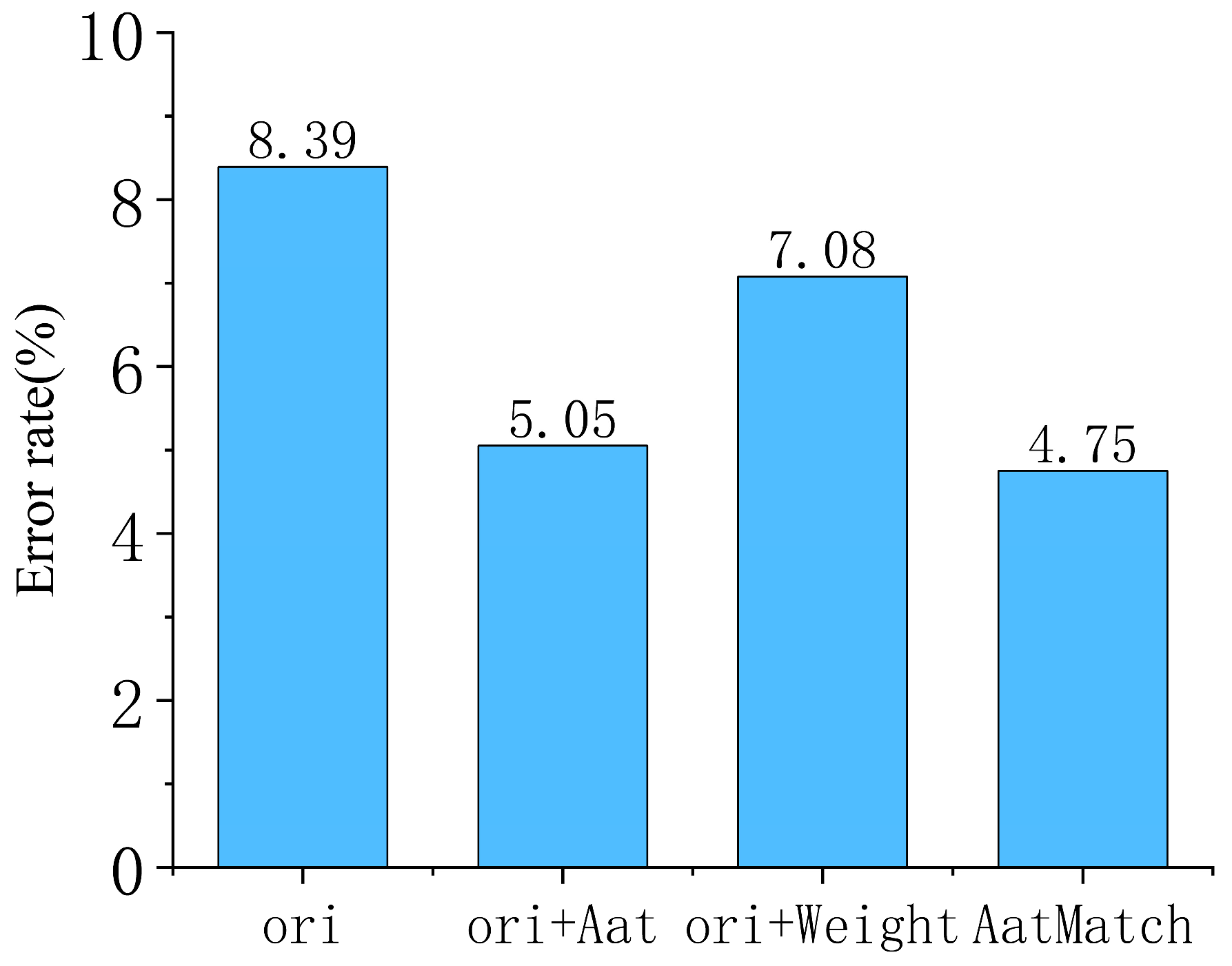
As shown in Figure 1, ‘‘ori’’ refers to the original model without any algorithmic components added. “ori+Adt” indicates the original model with the adaptive adversarial module added. In contrast, “ori+Weight” indicates the original model with the adaptive weight module added, the lack of any component of the algorithm AatMatch will make degradation of the model performance. The adaptive adversarial module achieves the most significant improvement in the model performance.

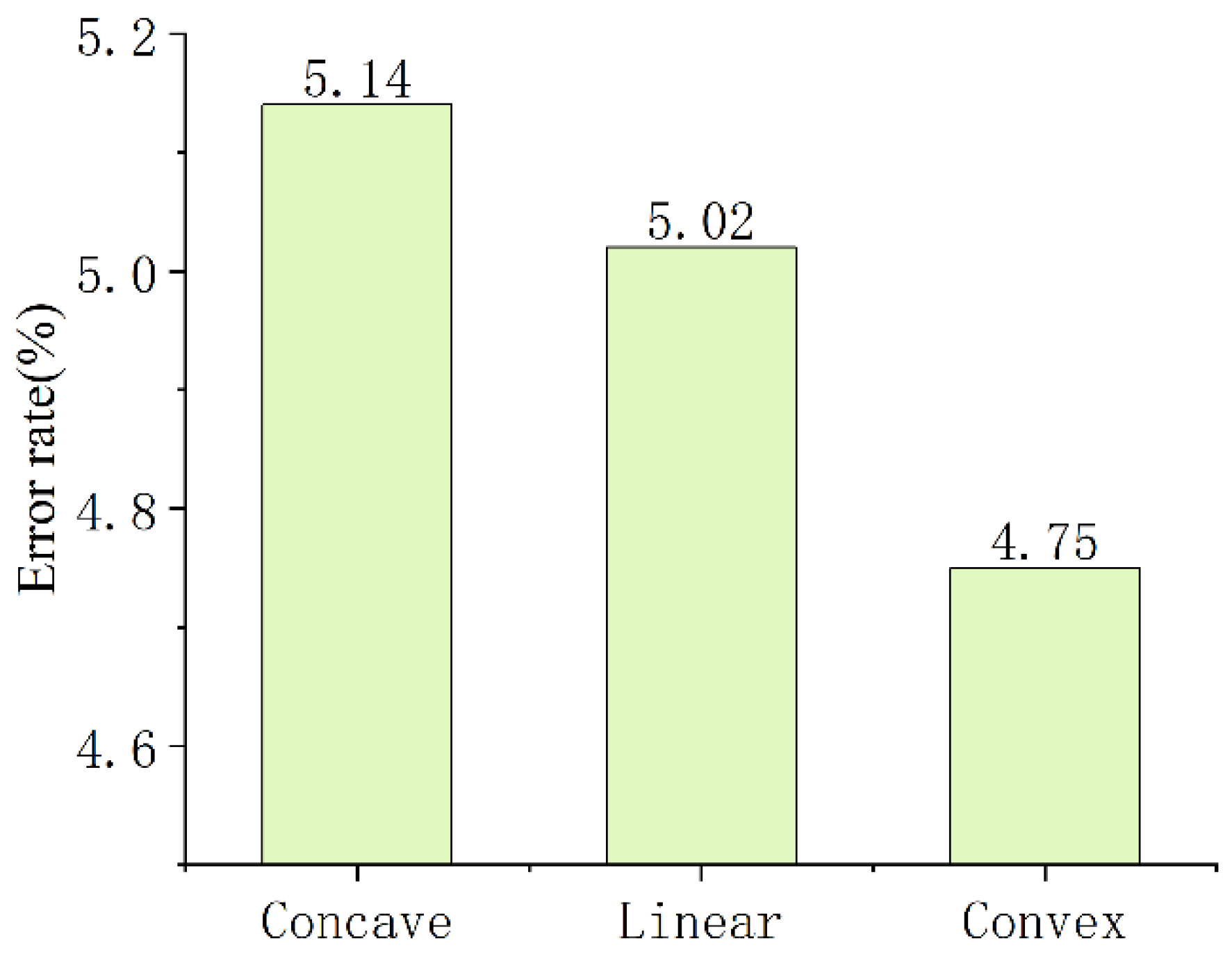
In Figure 2, we compare the performance of three different weight functions: the concave, linear, and convex functions. Our results indicate that the convex function outperforms the others, while the concave function performs worst. This outcome is because the convex function can more accurately distinguish the number of samples from classes with varying learning effects, ultimately leading to better classification results.

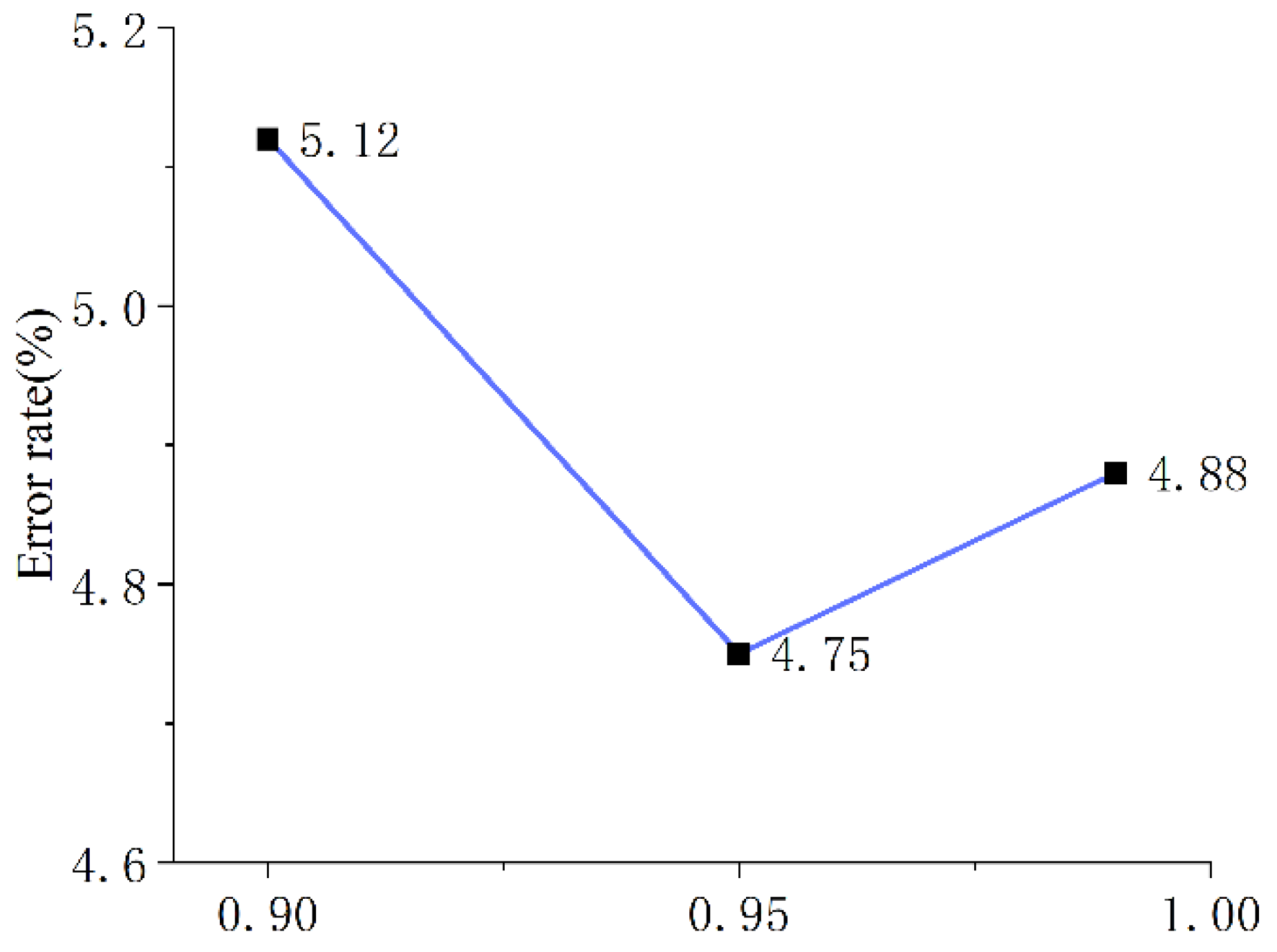
Based on the results shown in Figure 3, the optimal classification performance is achieved when the $\tau$ value is set to 0.95. If $\tau$ is too large, a significant number of samples will be filtered out, resulting in insufficient training data. On the other hand, if $\tau$ is too small, numerous low-confidence samples will be included in the training, thus impeding the model training process. Therefore, selecting the appropriate value of $\tau$ is crucial in balancing the training data’s quantity and quality, ultimately affecting the classification performance.

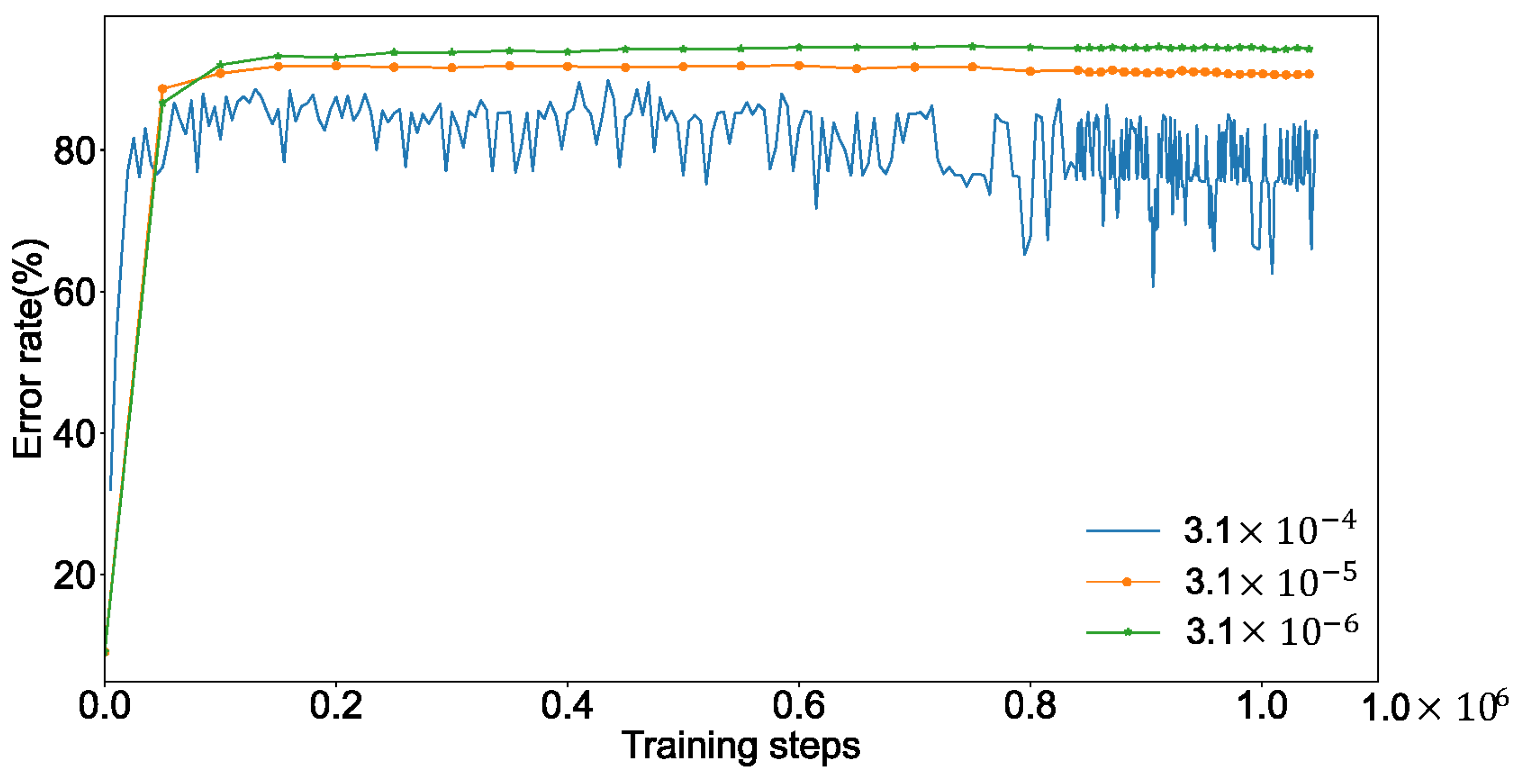
To explore the classification boundaries of low-density regions, adversarial perturbations are added to the images. However, ensuring that these perturbations do not produce adversarial samples misclassified as other classes is important. As shown in Figure 4, when the adversarial perturbation is too strong, it can cause a mismatch between the distribution of original data and that of adversarial data, which leads to the network learning wrong features from both domains and thus overfitting, ultimately reducing the model’s classification performance. A properly selected magnitude of adversarial perturbation can help improve the model’s classification performance. Specifically, the model achieved the highest accuracy when the inverse perturbation was set to $\epsilon$ = 3.1 × 10⁻⁶.

5. Conclusions

This paper introduces a novel semi-supervised learning algorithm, AatMatch, combining curriculum learning and adversarial training to act as a data augmentation method for generating adversarial samples. These samples are generated based on the learning difficulty of a category and are then utilized to explore the classification boundaries. A momentum model is incorporated to address the consistency problem of historical information effectively. Additionally, adaptive weights are assigned to each unlabeled data point based on its prediction confidence, thereby minimizing the negative impact of low-confidence data on the model’s performance. The proposed algorithm has demonstrated superior performance compared to existing advanced methods across various datasets.

References

- Schmidhuber, J. Deep learning in neural networks: An overview. Neural Netw. 2015, 61, 85–117. [Google Scholar] [CrossRef] [PubMed]
- van Engelen, J.E.; Hoos, H.H. A survey on semi-supervised learning. Mach. Learn. 2020, 109, 373–440. [Google Scholar] [CrossRef]
- Sindhu Meena, K.; Suriya, S. A survey on supervised and unsupervised learning techniques. In Proceedings of the 1st International Conference on Artificial Intelligence; Springer: Cham, Switzerland, 2020; pp. 627–644. [Google Scholar]
- Oliver, A.; Odena, A.; Raffel, C.A.; Cubuk, E.D.; Goodfellow, I. Realistic evaluation of deep semi-supervised learning algorithms. In Proceedings of the 32nd Annual Conference on Neural Information Processing Systems, Montréal, QC, Canada, 2–8 December 2018; pp. 3239–3250. [Google Scholar]
- Lee, D.-H. Pseudo-label: The simple and efficient semi-supervised learning method for deep neural networks. In Proceedings of the Workshop on Challenges in Representation Learning, Atlanta, GA, USA, 16–21 June 2013; Volume 2, p. 896. [Google Scholar]
- Sajjadi, M.; Javanmardi, M.; Tasdizen, T. Regularization with stochastic transformations and perturbations for deep semi-supervised learning. In Proceedings of the 30th Annual Conference on Neural Information Processing Systems, Barcelona, Spain, 5–10 December 2016; Curran Associates Inc.: Red Hook, NY, USA, 2016; pp. 1163–1171. [Google Scholar]
- Cubuk, E.D.; Zoph, B.; Shlens, J.; Le, Q.V. Randaugment: Practical automated data augmentation with a reduced search space. In Proceedings of the 33rd IEEE Conference on Computer Vision and Pattern Recognition Workshops, Washington, DC, USA, 14–19 June 2020; pp. 702–703. [Google Scholar]
- Wang, X.; Chen, Y.; Zhu, W. A Survey on Curriculum Learning. IEEE Trans. Pattern Anal. Mach. Intell. 2021, 44, 4555–4576. [Google Scholar] [CrossRef] [PubMed]
- Goodfellow, I.J.; Shlens, J.; Szegedy, C. Explaining and harnessing adversarial examples. In Proceedings of the 3rd International Conference on Learning Representations, Banff, AB, Canada, 14–16 April 2014; pp. 1–11. [Google Scholar]
- Laine, S.; Aila, T. Temporal ensembling for semi-supervised learning. In Proceedings of the 5th International Conference on Learning Representations, San Juan, Puerto Rico, 2–4 May 2016; pp. 1–13. [Google Scholar]
- Miyato, T.; Maeda, S.; Koyama, M.; Ishii, S. Virtual adversarial training: A regularization method for supervised and semi-supervised learning. IEEE Trans. Pattern Anal. Mach. Intell. 2018, 41, 1979–1993. [Google Scholar] [CrossRef] [PubMed]
- Tarvainen, A.; Valpola, H. Mean teachers are better role models: Weight-averaged consistency targets improve semi-supervised deep learning results. In Proceedings of the 31st Annual Conference on Neural Information Processing Systems, Long Beach, CA, USA, 4–9 December 2017; pp. 1195–1204. [Google Scholar]
- Verma, V.; Kawaguchi, K.; Lamb, A.; Kannala, J.; Solin, A.; Bengio, Y.; Lopez-Paz, D. Interpolation consistency training for semi-supervised learning. Neural Netw. 2022, 145, 90–106. [Google Scholar] [CrossRef] [PubMed]
- Zhang, H.; Cisse, M.; Dauphin, Y.N.; Lopez-Paz, D. Mixup: Beyond empirical risk minimization. In Proceedings of the 6th International Conference on Learning Representations, Vancouver, BC, Canada, 30 April–3 May 2018; pp. 1–13. [Google Scholar]
- Xie, Q.; Dai, Z.; Hovy, E.; Luong, T.; Le, Q. Unsupervised data augmentation for consistency training. In Proceedings of the 34th Annual Conference on Neural Information Processing Systems, Online, 6–12 December 2020; pp. 6256–6268. [Google Scholar]
- Rizve, M.N.; Duarte, K.; Rawat, Y.S.; Shah, M. In defense of pseudo-labeling: An uncertainty-aware pseudo-label selection framework for semi-supervised learning. In Proceedings of the 9th International Conference on Learning Representations, Virtual Event, Austria, 3–7 May 2021; pp. 1–20. [Google Scholar]
- Wang, X.; Gao, J.; Long, M.; Wang, J. Self-tuning for data-efficient deep learning. In Proceedings of the 38th International Conference on Machine Learning, Virtual, 18–24 July 2021; pp. 10738–10748. [Google Scholar]
- Berthelot, D.; Carlini, N.; Goodfellow, I.; Papernot, N.; Oliver, A.; Raffel, C.A. MixMatch: A Holistic Approach to Semi-Supervised Learning. In Proceedings of the 33rd Annual Conference on Neural Information Processing Systems, Vancouver, BC, Canada, 8–14 December 2019; pp. 5049–5059. [Google Scholar]
- Berthelot, D.; Carlini, N.; Cubuk, E.D.; Kurakin, A.; Sohn, K.; Zhang, H.; Raffel, C. ReMixMatch: Semi-Supervised Learning with Distribution Matching and Augmentation Anchoring. In Proceedings of the 8th International Conference on Learning Representations, Addis Ababa, Ethiopia, 26–30 April 2020. [Google Scholar]
- Sohn, K.; Berthelot, D.; Carlini, N.; Zhang, Z.; Zhang, H.; Raffel, C.A.; Cubuk, E.D.; Kurakin, A.; Li, C.L. Fixmatch: Simplifying semi-supervised learning with consistency and confidence. In Proceedings of the 34th Annual Conference on Neural Information Processing Systems, Online, 6–12 December 2020; pp. 596–608. [Google Scholar]
- Li, J.; Xiong, C.; Hoi, S.C.H. Comatch: Semi-supervised learning with contrastive graph regularization. In Proceedings of the 34th IEEE International Conference on Computer Vision, Virtual, 7–9 June 2021; pp. 9475–9484. [Google Scholar]
- Zhang, B.; Wang, Y.; Hou, W.; Wu, H.; Wang, J.; Okumura, M.; Shinozaki, T. Flexmatch: Boosting semi-supervised learning with curriculum pseudo labeling. In Proceedings of the 35th Annual Conference on Neural Information Processing Systems, Virtual, 6–14 December 2021; pp. 18408–18419. [Google Scholar]
- Yang, F.; Wu, K.; Zhang, S.; Jiang, G.; Liu, Y.; Zheng, F.; Zhang, W.; Wang, C.; Zeng, L. Class-Aware Contrastive Semi-Supervised Learning. In Proceedings of the 35th IEEE Conference on Computer Vision and Pattern Recognition, New Orleans, LA, USA, 18–24 June 2022; pp. 14421–14430. [Google Scholar]
- Zheng, M.; You, S.; Huang, L.; Wang, F.; Qian, C.; Xu, C. Simmatch: Semi-supervised learning with similarity matching. In Proceedings of the 35th IEEE Conference on Computer Vision and Pattern Recognition, New Orleans, LA, USA, 18–24 June 2022; pp. 14471–14481. [Google Scholar]
- Krizhevsky, A.; Hinton, G. Learning multiple layers of features from tiny images. In Technical Report; Department of Computer Science University of Toronto: Toronto, ON, Canada, 2009. [Google Scholar]
- Netzer, Y.; Wang, T.; Coates, A.; Bissacco, A.; Wu, B.; Ng, A.Y. Reading digits in natural images with unsupervised feature learning. In Proceedings of the 25th Annual Conference on Neural Information Processing Systems Workshop on Deep Learning and Unsupervised Feature Learning, Granada, Spain, 12–14 December 2011; pp. 1–9. [Google Scholar]
- Zagoruyko, S.; Komodakis, N. Wide Residual Networks. In Proceedings of the 27th British Machine Vision Conference, York, UK, 19–22 September 2016; Richard, E.R.H., Wilson, C., Smith, W.A.P., Eds.; BMVA Press: York, UK, 2016; pp. 1–12. [Google Scholar]
- Loshchilov, I.; Hutter, F. Sgdr: Stochastic gradient descent with warm restarts. In Proceedings of the 25th International Conference on Learning Representations, San Juan, Puerto Rico, 2–4 May 2016; pp. 1–16. [Google Scholar]
Figure 1.
Ablation study of algorithm module.
Figure 2.
Ablation study of weight function.
Figure 3.
Ablation study of the parameter m.
Figure 4.
Ablation study of the parameter .