
Lifecycle Value Sustainment and Planning Mission Upgrades for Complex Systems: The Case of Warships

1
Navantia Australia, Melbourne, VIC 3008, Australia
2
STEM Engineering School, University of South Australia, Adelaide, SA 5000, Australia
*
Author to whom correspondence should be addressed.
Systems 2023, 11(4), 183; https://doi.org/10.3390/systems11040183
Submission received: 28 February 2023
/
Revised: 20 March 2023
/
Accepted: 30 March 2023
/
Published: 2 April 2023
(This article belongs to the Special Issue Simplifying the Complex: Modeling and Analysis for System Design and Management)
Abstract
:Changeability analysis methods primarily assist with formulating a response to uncertain and new requirements from various system stakeholders and include asset management issues such as modelling lifecycle path dependency. Epoch-era networks proved to be an effective tool for managing the evolving requirements of a capability system, ensuring sustained value through life. Over the life of a system, stakeholders are faced with countless options to change their capability systems to sustain value, which is path dependent and can greatly impact the scope of decisions available later in life. This paper introduces and demonstrates the application of a revised epoch-era network approach to explore many potential lifecycle paths, along with utility vs. expense strategies, demonstrated through an example of a military frigate subject to evolving requirements. Results indicated the future limitations to sustaining value if the largest and most capable technology upgrades are selected too early in life. The two best lifecycle paths from different strategies were compared to understand the utility/expense trade-offs for the most optimal frigate upgrade trajectory.
1. Introduction
Changeability is a characteristic of complex engineered systems for meeting the demands from evolving requirements [1,2]. Changeability seeks to ensure systems sustain their value by meeting new requirements within the desired cost. Changeability is a concept closely related to resilience which is the ability of systems to bounce back in the presence of disruptions. However, changeability, more accurately, is regarded as one of the contributing factors to the system resilience [3]. Systems with long service lives are likely to encounter changes from evolving technologies, fluctuating markets, new threats, varying needs, and shrinking budgets [1]. The value sustainment in the face of such changes can be seen as future-proofing [2,4]. The only certainty of these future requirements is their uncertainty. In a military context, for example, the future requirements change when strategic and tactical operational scenarios become updated based on geological force field topological evolution. Changeability concepts provide a risk mitigation strategy for appropriately managing such uncertainties through the life of a system [5]. Changeability concepts are enabled in systems via change mechanisms [6]. Change mechanisms such as modularity, interoperability, reconfigurability, and margins allow the physical change in a system to take effect [1]. For clarity, margins are design overspecifications concerning the minimum required requirements. Figure 1 shows the relationship between various changeability elements. To achieve changeability in systems, designers must consider factors such as modularization, flexibility, scalability, and maintainability. The design must be modular, allowing for components to be added or removed as needed, and must be flexible enough to accommodate new requirements. Additionally, the system should be scalable, able to adapt to changes in the size or complexity of the problem being addressed, and maintainable, allowing for easy updates and repairs. Modularity and flexibility are closely related factors that contribute to the changeability of a system. A modular system is composed of independent components that can be modified, replaced, or removed without affecting the functionality of other components. Flexibility refers to the ability of a system to adapt to new requirements or changes in the environment. A modular system is often more flexible than a monolithic system because it can be easily reconfigured to address new needs. Scalability has a close relationship with maintainability. A system that is highly maintainable is typically easier to change than a system that is difficult to modify. Scalability refers to the ability of a system to handle increases in complexity or size. A system that is highly scalable can adapt to changes in the problem being addressed. Systems that are both highly maintainable and highly scalable are often highly changeable because they can be modified and adapted to meet new needs. Note that the conceptualization presented here for changeability differs from those presented by [6,7]. For detail of these definitions as intended in this paper, see [1].
Changeability analysis methods have primarily focused on the design and development of new systems [2]. Entities such as the Australian Defence Organisation (ADO), however, express preference for purchasing existing systems such as warships, for which application of current changeability analysis methods may not be entirely suitable [2]. A key reason for employing changeability analysis on existing systems is to allow stakeholders to better plan and manage probable evolving requirements affecting the already acquired system. Knowing the response of a system’s built-in change mechanisms to various possible contexts and stakeholder preferences, stakeholders can select the best set of proposed new requirements that can be feasibly met by the system. Abstracting this process over the life of a system enables lifecycle path analysis; whereby, stakeholders can plan the path a system follows throughout its lifecycle in response to feasibly meeting new demands and expectations, ensuring sustained value over the utilization phase of life.
Some value optimisation models can be used for future systems only such as that in [8] which is based on System Readiness Levels (SRL), or to both future and existing systems such as Epoch-Era Analysis (EEA). EEA pioneered by Ross and Rhodes [9] can form a foundation to facilitate lifecycle path analysis of in-service systems [1,2]. An epoch is a time period bounding a singular set of contexts and stakeholder preferences [7]. Likewise, an era is the stringing together of epochs to form a representative system lifecycle identified by a significant change of context [7]. Several hindrances may be observed when applying EEA for lifecycle path analysis of already in-service systems. These hindrances relate to the significance of system path dependence, essential to lifecycle path analysis. Indeed, the concept of path dependence has been briefly introduced in seminal work of Ross [7]. However, there is still a gap in applying such a concept to in-service systems, a goal that this paper aims to achieve.
To our best knowledge, no paper has addressed the issue of applying changeability analysis to existing systems which can be challenging due to several reasons:
- (1)
- Existing systems may not have been designed with changeability in mind. When a system is designed and implemented, the design choices made at that time can limit the ability of the system to change or evolve over time. These limitations may not become apparent until the system needs to be modified, and the cost of making these modifications can be high.
- (2)
- Existing systems may not have been well-documented, making it difficult to understand how the system works or how changes might impact the system. This lack of documentation can make it challenging to identify areas of the system that are most in need of change or to understand how changes might impact other parts of the system.
- (3)
- Another factor that can make it difficult to apply changeability analysis to existing systems is the lack of a clear understanding of the system’s requirements or the environment in which it operates. If the system’s requirements or operating environment have changed since the system was designed, the original design may no longer be appropriate, and changes may be required to ensure that the system continues to meet its intended goals.
- (4)
- The cost of making changes to an existing system can be high, both in terms of time and resources. This cost can make it difficult to justify making changes to the system, particularly if the benefits of those changes are not clear.
These factors overall render the system sensitive to the path or order of implementing system changes. Path dependence is critical to the appropriate analysis of certain in-service systems, such as warships. Path dependence can be studied at tactical or strategic levels. At the tactical level, optimum mission planning is essential for minimizing the cost and maximising the utility [10]. At the strategic level, warships experience a change to their physical characteristics once modified. For example, the addition of a new weapons system increases the ship’s mass, which in turn, affects the overall ship’s performance. Hence, the system baseline characteristics change through time in an ordered manner, and therefore its performance against evolving requirements is path-dependent. To suitably perform lifecycle path analysis on in-service systems, all conceivable lifecycles must be analysed to better inform stakeholders. Epoch-era networks can assist stakeholders in appropriately managing and planning the lifecycle path of an in-service warship once acquired. Guided by short- or long-term design strategies, such as maximising system utility, stakeholders can identify optimal lifecycle paths that respond effectively to evolving technological and operational requirements. In this manner, epoch-era networks can provide evidence-based advice for warship upgrades, redesign, or new operational requirements that can be feasibly met by the warship’s margins, ensuring current and future sustained value.
This paper proposes and demonstrates a network-driven approach to capture system path dependence with the application of EEA to perform lifecycle path analysis on an in-service warship. In linking a series of upgrade paths progressing sequentially through epochs, a lifecycle path can be developed. A representation of all potential lifecycle paths for a single warship form what is referred to herein as an epoch-era network. System dependency is explicitly accounted for within epoch-era networks since the end of one upgrade path from an epoch forms the new baseline design from which the next upgrade path follows in the subsequent epoch.
The rest of this paper is organized as follows: Section 2 provides a background literature review on system changeability within the context of various engineering industries; Section 3 details the revised method for application with in-service systems and introduces the epoch-era network; Section 4 is a demonstration case study followed by results and discussion about various implementable strategies in Section 5; the paper concludes in Section 6.
2. Background
Asset Management (AM) includes activities to support effective decision-making that optimises the service delivery potential of an asset whilst minimizing risks and costs throughout their service lives [11]. Frolov [11] states that historically these activities focus on decisions related to system maintainability, reliability, and availability. Extending this notion, El-Akruti [12] recommends that AM should be applied more holistically encompassing all lifecycle activities. These activities should include those that support system improvements or upgrades to maintain or improve service delivery or performance [13]. Such outcomes are like those achieved by performing changeability analysis on in-service systems. However, the AM literature is not rich with activities comparable to changeability analysis that can help ensure the sustained value of an asset through life. In this sense, the proposed outcomes of changeability analysis in this paper complement holistic AM activities.
Implementing changeability into system architectures was a concept originally idealized by Fricke et al. [14] to efficiently manage changes in needs and requirements over the lifespan of a system. Such changes typically result from dynamic marketplaces, technology evolution, and varying environments [5,15]. In response to such changes, changeability may be defined as the ability of a system to alter its state to meet new requirements and/or expectations [2]. Through altering states, the system may change form, function, or operation. Change is a necessary response enabling the system to sustain value, as opposed to becoming obsolescent [1,16]. Changeability is achieved according to a semantic set of system characteristics and “-ilities” commonly including, but not limited to flexibility, adaptability, robustness, scalability, modifiability, margins, interoperability, reconfigurability, and modularity [1,16].
Literature regarding this semantic set has largely emerged as an ambiguous discourse for a common definition and application of each -ility, and their relationships to each other [17]. Aiming to remove these ambiguities, Ross and Rhodes [9] introduced the change agent-effect-mechanism framework providing a suitable foundation for appropriately defining and applying changeability and its many interrelated concepts. In this framework, flexibility and adaptability are distinguished by either an external or internal agent, respectively, regarding their location to the system boundary, initiating the change in the system [6]. For example, [18] related the flexibility of a fleet of aircraft to their reliability and availability. Instigating a change affects the design parameters comprising a system in some quantifiable way. [6] further categorize these effects as either robust, scalable, or modifiable resulting in a system where the design parameters: remain constant, are individually increased, or are added to/subtracted from the set, respectively, in response to meeting new requirements.
Of more importance to the application of changeability are the change mechanisms that physically enable the change effects to be realized. Dwyer [1] identifies a common set of change mechanisms of relevance to engineered systems including margins, interoperability, reconfigurability, and modularity; further details on each of these change mechanisms can be found in [19,20,21,22], respectively (see Figure 1). Each mechanism facilitates a distinctive set of path enablers (change paths) comprising associated conditions, resources, and constraints available to the system [9]. For example, if the margin is the mechanism, then a weight margin is the path enabler. Additionally, specific low-level transition rules may be defined for each path enabler. A transition rule for a weight margin path enabler may be fuel storage weight growth. Transition rules affect and therefore provide a direct mapping to design parameters [6]. In this manner, the impact of transition rules on the system architecture, and therefore its performance, can be determined.
2.1. Changeability Analysis Methods
Changeability analysis methods have evolved alongside the increasing need to model uncertainties associated with requirements creep and operational scenario changes affecting the value of complex engineered systems over their service lives. A widely adopted method for commercial applications is Real Options Analysis (ROA). ROA is commonly used to financially value the inclusion of incorporating changeability into the design of engineered systems [23,24,25]. Nonetheless, ROA oversimplifies the problem of changeability analysis, inheriting many assumptions from its roots in financial theory, reducing its applicability to the physical systems [26]. Change Propagation Analysis (CPA) has also emerged as an adequate option for identifying high-value change mechanisms [19,27]. However, CPA is limited to investigating a small number of change events and is unable to suitably perform lifecycle path analysis.
A promising and recently well-adopted method is the Responsive Systems Comparison (RSC) method proposed by [28]. The RSC method combines Multi-Attribute Tradespace Exploration (MATE) and EEA, into a step-by-step approach. MATE is a conceptual design method combining multi-attribute utility theory and Tradespace exploration to aid in the evaluation of many system designs based on performance (utility) and cost attributes [29]. EEA provides a temporal extension to the traditionally static context and preference-orientated MATE method [30]. This is achieved by capturing a snapshot of context and preference-derived design requirements in a single epoch (epoch variables), and sequencing epochs together (forming a system era) to produce a time-orientated framework whereby methods such as MATE can be operationalized throughout [9]. The first iteration of the RSC method contains a set of seven processes designed to guide the analyst through various insights regarding changeability and sustained value; they are [28]: (1) context definition—identify the problem/needs statement and important contextual factors; (2) design formulation—elicit the stakeholder needs statement (attributes) and formulate system concepts (design variables); (3) epoch characterization—parameterize key contextual and perceptual uncertainties to produce epoch variables; (4) design Tradespace evaluation—develop knowledge via modelling and simulation of how design variables map to system concepts and attributes producing value in response to the context and perceptions of an epoch; (5) multi epoch analyses—the performance of many system concepts is evaluated across many contexts and preferences; (6) era construction—system eras are constructed from the sequencing of static epochs to evaluate concepts in dynamic contexts and preferences; (7) lifecycle path analysis—strategies for ensuring systems can maintain value over lifecycles (eras) are produced.
Schaffner, et al. [31] extended the RCS method, analysing system concepts in single epochs, single-eras, and multi-eras more explicitly and comprehensively. While [32] develops these processes into new steps, they may also be recognized as sub-steps as part of wider scoped epoch-analysis and era-analysis steps. Furthermore, [32] omits lifecycle path analysis, integrating this process into multi-era analysis, and reducing its effectiveness as a standalone process for identifying the optimal path a system shall follow in response to uncertain lifecycle demands.
The Filtered Outdegree (FOD) method in various forms which treat the traditional Tradespace as a network has been used effectively to complement the RSC method [33,34]. The Tradespace network comprises nodes and arcs representing system concepts and transition paths, respectively. A path allows a concept to change from one state to another via a transition rule. Applying cost/resource thresholds to arcs, the outdegree of a node (the number of feasible paths it can take) can be filtered. The Tradespace network concept is a critical enabler in effectively performing lifecycle path analysis. The method provides a means for explicitly modelling system path dependence by linking all possible system end states through many potential lifecycles, thus facilitating the development of an epoch-era network.
2.2. Applying Changeability Analysis Methods to In-Service Systems
Applications for changeability analysis of engineered systems are often biased toward the design and development of new systems. Ross and Hastings [35] applied the FOD method to the design of a satellite, weapons system, and an on-orbit observatory. Refs. [33,34] utilized EEA and a modified FOD measure to support the design of a highly changeable satellite radar system. Fitzgerald et al. [26,36] employed EEA and a set of Pareto-based metrics to select a single or set of space-tug designs that can maintain a high value. Refs. [37,38] applied the FOD concept and EEA, respectively, to explore the benefits of various path enablers in improving the changeability of a commercial ship for increased value. To the best of our knowledge, EEA was never conducted for an existing system, which is a novel contribution of this paper. In this paper, the characteristics below are considered in a changeability analysis framework:
- System path dependence: akin to the butterfly effect, the lifecycle path of an existing system is dependent on the system’s response to evolving requirements through time; had one system design decision been made differently, the system’s performance for its remaining service life may be drastically altered. Hence, it is critical to understand the consequences of all perceivable decisions. Since many decisions are available to stakeholders in response to a new set of requirements, decision-makers can only be sure of the best decision if all possible design alternatives and consequent lifecycle paths are understood. Applying this understanding, decisions that increase value in the short-term (e.g., major technology upgrade) though inhibit further increases in value in the long-term (e.g., consume all margins preventing future upgrades) can be avoided, allowing all decisions to be optimised for lifecycle value. However, the current state of the EEA (Ross & Rhodes, 2008) does not allow for a full enumeration of path-dependent system lifecycles. This work pays particular attention to path dependency, as an addition to the EEA framework.
- Issue of short-term underperforming designs: the generation of all possible lifecycle paths, dependent upon a proposed sequence of context and perception-driven requirements, yields many possible system end states. A subset of these system end states may underperform against a subset of contexts and preferences. In the traditional application of EEA, a strategy or goal is applied to each epoch individually [9]. The best performing system end state(s) for that strategy is (are) selected, initializing the creation of a new epoch to analyse the selected system state(s). In this manner, underperforming system end states are not analysed further, and stakeholders fail to gain knowledge of their subsequent performance in later epochs. It is possible that underperforming design options in the short-term evolve to become the best-performing designs in the long term. While [7,9] acknowledge this concept as an important consideration for the current state of EEA, the concept can only be suitably achieved through a full enumeration of path-dependent system lifecycles.
- Changing the change variables: The fundamental principle of changeability analysis implies that complex engineered systems need to change over time as a strategic response to maintain value. Such systems, however, change by adding/upgrading subsystems, which may be regarded as complex systems in their own right. For example, [32] and [35] applied changeability analysis to the conceptual design of a warship and missile system, respectively; albeit, the missile subsystem commonly evolves over the life of a warship. Factoring the rate at which subsystems change, i.e., their performance and physical specifications, is an important consideration to more accurately predict the impact of changes on a system. Accordingly, factoring subsystem changes compounds the importance of path dependence since the design parameters used for subsystem upgrades can become time-dependent. Combining system path dependence and the principles of change to both systems and subsystems in a single analysis can help rectify the hindrances of current changeability analysis methods. However, we emphasize that this work is not intended to consider all types of uncertainty. The only type of uncertainty of interest to this research is tactical uncertainty in operational scenarios of a system.
The next section proposes a revision of the RSC method with the aim of improving the overall applicability for supporting through-life changes to the asset and improving value sustainment. Historically, evaluations tend to only occur during the initial design phase, but assets such as warships often undergo smaller incremental changes without going through a complete EEA and Tradespace analysis. As there is also a strong likelihood that initial assumptions/variables have become clearer, better known, and less ambiguous (due to the passage of time), it is proposed that the revised RSC method would provide better up-to-date results throughout the lifespan of the asset, and potentially better prepare the warship for future epochs-related requirements.
3. RSC Method: Epoch-Era Networks
Ross, McManus, Rhodes, Richards, Hastings and Long [28] and Schaffner, Shihong, Ross and Rhodes [31] formed the design Tradespace by process steps such as need and context identification (mainly through interviews), attribute definition, and finally epoch characterization of various designs. Here we present the RSC method with new process steps added to be applicable to existing systems. The focus of the revised method herein is on the new processes/steps that account for analysing requirements unique to existing systems and resolving current analysis hindrances introduced in the previous section. Figure 2 illustrates the revised RSC method which has eight high-level steps grouped into three modules for a better understanding of the process:
- Information gathering;
- Alternatives evaluation;
- Design analysis.
The revised method includes new steps and feedback loops related to the entire information-gathering stage and also in the design analysis stage related to path dependence. Next, we discuss further the steps of the revised RSC.
3.1. Information Gathering
Concerning existing systems, the RSC activities performed during step 1 focus on defining stakeholder needs regarding the proposed set of contexts the system is likely to operate within over its service life. Likelihoods and preferred sequencing of contexts are identified. Furthermore, stakeholder value propositions are elicited, providing a guide on how value is referred to according to the system’s response to changing contexts. Resources available to each stakeholder are identified forming resource thresholds for which the feasibility of system configurations (new system end states) is assessed.
Existing systems, to various degrees, have already been subject to the design formulation process of step 2.2. As such, their attributes, utility, and expense functions have previously been established. Therefore, the design definition process of step 2.1 involves identifying the presence of any new performance attributes concerning stakeholders in response to the existing system changing states. Importantly, this process requires the identification of path enablers and transition rules present in the existing system. New attributes should capture the system’s ability to meet original expectations. Revised utility functions are defined for these attributes depicting stakeholder preferences. Similarly, expense functions are defined from stakeholder resources, including those required to execute identified transition rules. Next, system configuration concepts are proposed enabling the identification of Design Variables (DVs) and subsequent ranges for each variable. The impact of system path dependence is defined in this step. Stakeholders must identify the path-dependent DVs throughout changing epochs. For example, an obvious path-dependent DV is system mass. To better understand this, stakeholders should consider this question: does the value of a DV depend upon the state of the system at the culmination of prior contexts and needs? If so, this affects how Epoch Variables (EVs) are mapped to DVs in the following steps.
Utilizing the contextual uncertainties and value propositions captured from step 1, specific future contexts that will affect the value of the system are developed in step 3. EVs are parameterized from high-level context-specific scenarios and associated preferences. EVs are typically decomposed by a high-level uncertainty category, a lower-level variable identifier, enumerated range/levels, and units. If an EV is subject to change as time progresses, the rate at which the EV changes can be factored into EV ranges/levels. This can be achieved using a growth factor altering the EV level within an epoch concerning the progression of epochs and their duration. If system path dependence must be modelled, the EVs that affect path-dependent DVs must be identified. For example, an EV for upgrading subsystem hardware will affect the system’s mass (the DV). These EVs and DVs will be modelled uniquely in the following step.
3.2. Alternatives Evaluation
Tradespace evaluation for existing systems is almost identical to that of new systems, whereby, step 4 in Figure 2 utilizes modelling and simulation to map DVs and EVs to system utility and expense attributes. Transition rules are used to link various system configurations by way of altering DVs to synthesise new configuration concepts in response to EVs. For existing systems, resultant utility and expense functions can then be used to generate a utility vs. expense Tradespace comprising unique system configurations. The basic process of generating each Tradespace for an existing system is illustrated in Figure 3, which utilizes two models, respectively, for utility and expense. The utility model is a model developed in the wider context of warfighting given the most likely future battle scenarios. A series of warfighting models and future scenarios have been developed in the Department of Defense. The authors were able to utilize the model related to maritime operations to produce the results reported in the following sections. The cost model utilized here is also developed in-house at the maritime unit of Defense Science and Technology Group (DSTG). The cost model is generic and applied to many different types of battleships taking into account maintenance costs and available resources in various locations in Australia.
Where the existing system is path-dependent, the state of system configurations and their respective DVs in the previous epoch must be carried forward, forming a baseline set of DV values from which the new Tradespace is generated in response to new EVs, further discussed in Section 3.4. While step 4 is critical for correctly developing simulation models suitable for the Tradespace construct, the static context view of Tradespace evaluation limits the ability to gain valuable changeability analysis insights of an existing system. Rather, these are achieved within the processes of design analysis.
3.3. Design Analysis
Design analysis comprises a set of processes by which the effects of various epochs on systems are analysed, as noted in Figure 3. Each of these processes allows the analyst to gain exclusive insights into the changeability behaviour of a system. Era construction involves several general processes as detailed by Roberts, et al. [39]. The first of these is to define durations for the system era and epochs. Era durations should depict the typical cradle-to-grave lifecycle of the system, or the remaining service life of the system if it is already operational. Epoch durations should depict the speed at which EVs change. Some EVs evolve at different rates to others, e.g., software and hardware are updated in the order of months and years, respectively. Here, it is important to ensure the rate at which subsystems change is modelled. Another approach to determining epoch durations is to use the historical rate at which similar systems have been upgraded/modified, e.g., typical warships undergo major upgrades every 7–10 years. Stemming from this process, it may be necessary to establish an epoch transition logic. The final process involves the structured ordering of epochs to form an era. Here, the analyst can employ direct or indirect approaches utilizing expert opinion or mathematical logic, respectively.
Using the era(s) constructed in the previous step, lifecycle path analysis in step 8 includes the assessment of various lifecycle strategies to ensure sustained value through life. The outcome of this process for existing systems is to provide stakeholders with a design/upgrade trajectory for the system that can ensure desirable performance against finite resources. Aiding this outcome, step 8.1 includes the analysis of various short- and long-term strategies to compare the cost benefits of employing such strategies. Understanding the long-term performance of short-term best and worst designs can be advanced in step 8.1. Likewise, the impact of resource and/or utility and expense attribute thresholds can be established. Insights gained from understanding the causes for a sub-optimal utility or increased expenses can be used to identify the most optimal lifecycle path, step 8.2. The value optimisation process includes the identification of a lifecycle path (or paths) that optimises the value of the system concerning the preferred (maybe tailored) strategy, resource thresholds, utility, and expense attributes. Enabling the analysis outcomes of step 8, epoch-era networks are proposed as a solution to model the full enumeration of all possible lifecycles for a path-dependent system.
3.4. Constructing and Analysing Epoch-Era Networks
The development of a single Tradespace was detailed in Section 3.2, repeating this process for each sequenced epoch defined from step 6, and utilizing the Tradespace network, an epoch-era network that can be produced according to Figure 4a. Due to system path dependence, the DVs comprising each system configuration in one epoch must be carried forward to the next epoch. This forms the new baseline set of system states subject to new configurations, in response to EVs, in the new epoch. Over the sequencing of multiple epochs, each Tradespace becomes networked by linking respective system configuration evolutions via transition rules, as depicted in Figure 4b. Fully enumerating all possible configuration options and considering all feasible combinations of EVs and their levels in each epoch results in a network growing exponentially as the era progresses.
To alleviate this problem, epoch-era networks can be analysed appropriately with the application of Shortest Path (SP) algorithms to successfully implement the processes of step 8. Using SP algorithms allows for showing only optimal paths between the existing system and all possible future states, thus reducing the total number of paths in consideration significantly. This way Figure 4c contains only the shortest paths between feasible states which subsequently has the structure of a tree graph. The SP problem is a well-studied combinatorial optimisation problem [40] that is also relevant to this investigation as these algorithms can provide a means for assessing and ranking various lifecycle strategies from which optimal paths can be identified and scrutinized further [2].
The Dijkstra algorithm [41] is a reliable SP algorithm employed here to identify the shortest distance between a destination node and every other node within a network. The shortest path is calculated based on arc properties such as weights, which may represent the cost of a system, to transition states. Weights may also depict differences in utilities between system states, or any other system attribute(s) part of the analysis. Adjusting the arc weights for varying lifecycle strategies within an epoch-era network, the most optimal lifecycle paths can be identified.
4. Case Study
RSC method is generic and can be applied to any existing system. Here, we follow each step specified in the previous section. The most important challenges in applying this method to any system as demonstrated here for the case of frigates are as follows:
- (1)
- Acquiring information about system parameters (that are usually well documented for defence systems and not so well for other systems) is a challenge;
- (2)
- Assessment of cost of changes might not be knowable a priori in the case of some systems. This is because changes are not planned in advance for some existing systems, so the cost issue becomes a major challenge;
- (3)
- Assessing the value of changes relative to future requirements is also a major challenge. Here, we demonstrate the value evaluations for three neatly defined requirements that are gearing the vessel for anti-air and anti-submarine operations. However, these requirements might not be as clear for other systems and might be accompanied by ambiguities which make the changes in value estimation challenging.
For this case study, the revised RSC method from Figure 2 is applied to an existing generic frigate. Warship upgrade planning is one of the costliest activities carried out by the defence. To this end, any cost savings that may also increase the utility of the warships is of huge interest both to the defence and the public. In this case study, we demonstrate exactly how this value optimisation and/or cost saving might be carried out during the planned upgrades of warships. The original baseline characteristics of the frigate are detailed in Table 1. For step 1, the frigate is subject to changing technological and operational requirements over an indicative 21-year service life. In this generic example, the frigate will be subjected to upgrades approximately every 7 years, which might be due to a change in operations, or a new operating environment. In this example, three epochs are considered: the first epoch between year 1 and year 7, the second epoch from year 7 to year 14, and the third epoch from year 14 to 21. Respectively, there are three planned technology gearing and upgrades the first of which takes place at year zero or before start of operation. Changes in operations and new operating environments are mandatory, while stakeholders have the option to install any combination of available technologies as part of an upgrade. Epoch-era networks are applied to determine the best set of lifecycle paths, or technology upgrade trajectories, for the frigate through the exploration of various utility/expense strategies and resource thresholds.
4.1. Transition Rules, Attributes and Design Variables
Transition rules that have been built into the existing frigate were identified first as part of step 2.1 to allow expense attributes to be mapped to their utilization. The frigate relies on margins as the key change mechanism comprising a set of path enablers accommodating changes to the system’s physical characteristics including mass, space, power, cooling, and data. Margins are excess or reserve capacities in design parameters that provide a buffer for absorbing change. Margins herein are either presented as the available value remaining or the limit of the design parameter until no further changes can be absorbed. For this case study, mass- and space-related margin enablers were employed. From the space margin path enabler, two transition rules were defined: (1) area margin—the available deck area for upgrading and adding new technology; (2) volume margin—the available compartment volume for upgrading and adding new technology. The availability of space margins for the frigate was defined in Table 2. From the mass margin path enabler, two transition rules were defined: (1) system mass margin—the maximum overall system mass allowable regarding strength limitations; (2) Vertical Centre of Gravity (VCG) margin—the maximum height of the frigate’s centre of gravity allowable regarding stability limitations. The upper limits to mass margins were defined in Table 2. Continuing step 2.1, single utility and expense attributes were defined according to Table 3 along with single-attribute weightings (ki) to produce Multi-Attribute Utility (MAU) and Multi-Attribute Expense (MAE) measures, respectively, according to (1) and (2):
where X is the set of attributes, Xi is the single-attribute level, N is the number of attributes, Ui(Xi) and Ei(Xi), respectively, are the utility and expense value functions for the ith attribute. Single-attribute utility and expense functions express a relationship between the attribute level (Xi) and level of goodness and are presented on a scale of 0 (worst) to 1 (best). Each single-attribute utility and expense function (excluding Technological Capability) was redefined for each epoch, representing a change in stakeholder preference. This resulted in a total of 19 separate functions which can be accessed by contacting the authors. Examples of single-attribute utility functions for resistance in epochs 1 and 3 are shown in Figure 5.
Note that the utility and cost models used here are linear in the sense that and are deemed as functions of only. A more comprehensive model should include reinforcing and negating effects of attributes on utility and cost. This means that, for example, should be a function of all Furthermore, this negation might render some paths incomprehensible. Here, we forego the assumption that such conflict between attributes exists.
Moving on, four utility attributes were defined: one about the frigate’s capability as a result of installed technology, and three about the frigate’s performance in an environment. The combination of technologies installed on the frigate, and their individual performance, provide the frigate with a weapons and sensor suite suitable to meet respective warfare capabilities. The more technologies installed and upgraded over all epochs, represented by a scale from 0 (none) to 1 (all possible), the better the technological capability of the frigate. A Sea Keeping (SK) utility is based on the frigate’s motion response in a certain sea state at cruising speed. A multi-criteria SK operability was used to determine the SK performance. A resistance utility was based on the frigate’s combined (calm water + added resistance in waves) resistance in a certain sea state at the cruising speed for head seas. A stability utility was based on the distance between the frigate’s VCG and Metacentric Height (GM); the greater the GM, the more stable the ship in general. The GM is affected by shifting VCGs and mass. Four expense attributes each relating to the consumption and remaining availability of margin-based transition rules were defined. A greater expense is attributed to greater consumption of margins since it is undesirable for stakeholders to consume more than the availability and limits of the margins. A 100% margin consumption would require a costly change to increase margins or add new change mechanisms. Weightings for the multi-attribute utility and expense measures are detailed in Table 3. A suite of physics-based ship performance models was used to simulate the frigates’ attributes based on a set of DVs [42].
Table 4 lists the design variables used to synthesise new system configurations that can achieve the defined utility attributes. The path-dependent DVs were identified and are notated by (a) in Table 4. Mass and VCG are both path-dependent variables that vary according to the number and locations of various installed technologies. All technologies are path-dependent because once installed, they become permanent and exhibit a level of performance respective to the time they were installed. Each technology was either already installed on the frigate and was therefore subject to upgrades or needs to be installed.
4.2. Epoch Requirements and Era Construction
The frigate is subject to changing capabilities, operations, and environments in response to evolving strategic military demands. Within step 3, thirteen epoch variables (EVs) were chosen from five uncertainty categories (derived from step 1) according to Table 5. Three warfare capabilities were each given a category: Anti-Submarine Warfare (ASW), Anti-Air Warfare (AAW), and Anti-Surface Warfare (ASuW). Each capability can be met by upgrading/adding respective technologies (the EVs) that fulfil that capability according to Table 5. The remaining two uncertainty categories reflect the ships’ operating conditions and environment, where it has been assumed there is an increased desire by stakeholders for ships to travel faster in larger seas. The EVs that also change specification as time progresses are denoted by superscript b in Table 5. These EVs are subject to both increasing mass and size growth factors as each epoch progresses.
Three distinct epochs were defined and sequenced to create a single frigate era for analysis for step 6, see Table 6. Epoch lengths were characterised as 7 years, representing a 21-year frigate service life. The full enumeration of EVs results in 7, 217, and 1519 unique frigate configurations for epochs 1, 2, and 3, respectively, considering system path dependence and neglecting the option to not upgrade/add any technology.
5. Results and Discussion
In this section we demonstrate the application of step 8 from the revised RSC method (Figure 2) using epoch-era networks to analyse the benefits and implications of various strategies, then use this gained understanding to identify preferred lifecycle paths from the best strategies. Due to high-level capability requirements for each epoch, an array of ASW, AAW, and ASuW technologies can be upgraded/installed, forming new configurations (herein denoted by “C”) in new epochs (denoted by “E”) according to Figure 6. For lifecycle paths, the notation C0.X.Y.Z has been adopted throughout the remaining section, where: C0 references the original baseline design; X, Y, and Z denote configuration options for epochs 1, 2, and 3, respectively, and represent the path-dependency of configurations through time. For example, C0.1.2.3 represents a ship that upgraded the torpedoes for ASW in epoch 1, upgraded main gun ammunition for AAW in epoch 2, and added harpoon missiles and launchers for ASuW in epoch 3.
Utility versus expense scatter plots for all configurations were created for the three epochs in Figure 7. The colour of each configuration represents the evolution of configuration alternatives branching from epoch 1 configurations. It can be seen that the variation in MAU and MAE for each configuration increases from epoch 1 to 3. This is expected since there is an order of magnitude number increase in the number of configurations in the following epoch due to system path dependency. Furthermore, configurations experience a wider variability of expense in epoch 3; this is likely due to configuration evolutions approaching margin limits where respective expenses increase by a greater amount.
The Pareto front is highlighted in each epoch showing the non-dominated solutions that exist along an optimal utility–expense trade-off line. Configurations on the Pareto front range between the most utility for a given expense, and the least cost for a given utility. Applying Pareto front analysis to the scatterplot from Figure 7, the best configurations through time based on various lifecycle strategies are limited to Pareto optimal solutions. However, due to system path dependence, the best lifecycle path resulting from a tailored strategy may not include a Pareto solution from any or all epochs, as explored next.
Figure 8 lists the configuration options, and their evolutions, which result in Pareto front solutions within a specific epoch. For this case study, the path dependency and changing stakeholder requirements lead to several sub-optimal configurations, E1C1, E2C11, and E2C23, to produce optimal evolutions in the following epochs. The opposite occurs for E2C4 and E2C15 as their evolutions become suboptimal in the following epoch, given that they were optimal in their current epoch. This demonstrates that for changeable systems, it is unreasonable to select designs against a set of static requirements (within a single epoch) since evolutions of that design against evolving requirements (over multiple epochs) can increase/decrease their value. Currently, suboptimal designs may prove of higher value to stakeholders against future requirements, and vice versa. This complex phenomenon demonstrates the significance of change mechanisms and how they enable value under uncertainty. Using information from Pareto optimal solutions in Figure 8, a stakeholder could have chosen E1C3 or E1C5 on an almost equal basis, or a stakeholder may not have chosen E2C15 on the basis that its configurations’ evolutions in epoch 3 do not result in optimal solutions. That same stakeholder would not be able to confirm if present design decisions were best in regard to meeting evolving requirements and changing preferences against all other possible lifecycle paths available to the frigate. Furthermore, the stakeholder would not be able to understand using just Pareto front analysis why one path is better than another. Hence, applying shortest path algorithms to epoch-era networks must be adopted to ensure the best set of system lifecycles against evolving requirements and changing stakeholder preferences which can be identified.
The resultant epoch-era network gives the range of possible ASW, AAW, and ASuW technology upgrade combinations proposed for each epoch, respectively. At the end of epoch 3, 1743 unique lifecycle paths for the generic frigate are possible. Via the network representation, weightings (W) are applied to edges connecting two nodes. Weightings represent the cost benefit of certain lifecycle strategies based on the MAU and/or MAE of each configuration (node) in each epoch. Summing the weightings between linked nodes through epochs allows the best possible lifecycle paths to be identified using the shortest path algorithms such as the Dijkstra algorithm. Note that although all states at the end of epoch 1 are distinct, the same is not true for states at the end of epochs 2 and 3.
5.1. Strategy Analysis: Maximising Utility
Figure 9a shows the results of determining the top 10 best paths for maximising the frigates’ lifecycle utility as part of step 8.1 from Figure 2. To make the lifecycle utility strategy suitable for the application of the Dijkstra algorithm, the edge weightings in the epoch-era network are determined using (3), where Wj is the weighting for the jth edge and MAUj denotes the MAU of the jth configuration.
Figure 9a shows only the optimal lifecycle paths. In this Figure, the thickness of the line represents edge weights and the most optimal path to achieving the chosen lifecycle strategy. All lifecycle paths in Figure 9a are in lieu of the stakeholder’s constraints for utility and expense attributes. Additionally, the numbering of the nodes follows the convention described at the start of Section 5. As expected, without consideration for expense attributes, the biggest upgrade configurations in general were selected in each epoch. Furthermore, Figure 9a suggests that the selection of bigger upgrades in earlier epochs contributes greatly to increased overall utility. This is evident since only C7 was selected in epoch 1. In epoch 2, C27, C29, and C30 containing four technology upgrade options and C31 (the maximum upgrade option) containing all five options (refer to Figure 6) were selected. Finally, a larger range of upgrades were available in epoch 3. This trend is logical because paths from Figure 9a represent ship upgrade trajectories that have the most frequently upgraded and therefore most capable technologies. However, this increase in capability must come at a cost. The difference in the overall mass of the ship due to different technology upgrade trajectories results in the best lifecycle path, C0.7.31.7 from Figure 9a, being 36 tons heavier than the worst lifecycle path, C0.7.31.4. Increased mass typically negatively affects performance and consumes margins. Since no constraints were applied in Figure 9a, every possible upgrade option for the frigate was available to the stakeholders.
In terms of the epoch-era network, this meant that for every configuration (node) in one epoch, all possible configurations (nodes) in the next epoch were available. The possibility to reach new nodes from a source node is referred to as an outdegree, as described before. Applying thresholds to the utility or expense attributes associated with each new node allows the filtered outdegree concept to be implemented with epoch-era networks. This allows stakeholders to tailor strategies to ensure performance or margin constraints are not being violated.
Applying an upper threshold to the maximum height of the frigate’s vertical centre of gravity (VCG) from Figure 9a, a typical physical limitation for ships, a significantly different set of best lifecycle paths occurs. In Figure 9b where the VCG filter is applied, only one lifecycle path from Figure 9a remains below the physical limitation for the frigates’ maximum VCG. Interestingly, C4 was selected in epoch 1 and was not identified as a Pareto optimal solution in Figure 7. This shows that the application of the epoch-era network allows the identification of a larger set of potential optimal design decisions against changing stakeholder preferences, or imposed constraints. Results from Figure 10a demonstrate the long-term impacts of choosing the best set of design decisions against a static view of the requirements and preferences when physical constraints are applied. From Figure 10a, the maximum configuration option that can be feasibly selected in epoch 3 to maximise utility over the entire lifecycle was C3. Hence, the most capable ASuW upgrade option for stakeholders was restricted to only upgrading one technology item. Compared to being able to upgrade all the frigate’s radar, automatic weapons system, and harpoon missile capability for the best possible ASuW capability, a strategy to maximise utility across all epochs significantly limits the frigate ASuW capability in epoch 3. Instead, the strategy can be tailored to emphasize certain attributes in a particular epoch.
Figure 10a shows the resultant lifecycle paths if stakeholders were to modify the proposed strategy of maximising overall utility and try to especially maximise the frigate’s ASuW capability in epoch 3. To maximise the utility in the final epoch given the VCG constraint, Figure 10a indicates that it was more beneficial to consider smaller technology upgrades in epoch 2. This is evident by comparing epoch 2 configurations between Figure 9a,b, where there is no option to upgrade the VLS and Seasparrow missiles (a major upgrade) in Figure 9b. This shows that certain upgrades have a far greater impact on certain constraints. However, if stakeholders decide the VLS and Seasparrow missiles must be upgraded in epoch 2, options exist to adjust constraints and enable the upgrade. For example, stakeholders could consider modifying the capacity of existing change mechanisms; adding new change mechanisms or easing constraints is explored next.
Easing constraints increases the number of reachable design alternatives available to each configuration for the following epoch. This number is referred to as the outdegree for each node within the epoch-era network. Figure 11 demonstrates the effect of easing restrictions on the outdegree for a sample of the nodes already discussed before. Given the original VCG constraint, relaxing this constraint by 0.15% and then again by 0.3% greatly increases the outdegree of epoch 2 nodes. For all epoch 2 options stemming from C7 in epoch 1, i.e., C0.7.1-31, the total number of epoch 3 configuration options increased by 24 after relaxing the constraint by 0.3%. Within this new set of 24 ASuW configuration options, stakeholders may identify a better lifecycle path as opposed to those identified in Figure 10a. Furthermore, the process of relaxing constraints represents the ability to alter the level of changeability a system such as a frigate possesses. For example, if the 0.3% relaxation in constraints was justified by modification or addition of a change mechanism, such as adding ballast to the frigate, then in turn this would result in an increase in the changeability level inherent to all frigate configurations present in epoch 2, and in general the baseline frigate itself.
Extending the lifecycle strategy followed in Figure 10a,b illustrates the revised best lifecycle paths had the VCG constraint been relaxed by 0.3%. Interestingly, the revised top 10 paths stem from the biggest epoch 1 ASW upgrade (C7). While relaxing the constraint ensures that the ASW capability can be maximised, it also allowed the VLS and Seasparrow missile upgrade options to be considered in epoch 2. Importantly, comparing the best lifecycle paths from Figure 10a,b, which is configurations C0.7.28.5 and C0.7.27.5, respectively, the overall utility for the best lifecycle path improved by ~7% after relaxing the constraint by 0.3%. This demonstrated the significant improvement in capability that can be achieved by altering the system’s changeability level. Finding Pareto optimal solutions using constraint relaxation requires testing for Karush–Kuhn–Tucker conditions [43], which is development beyond the scope of this paper, and will be considered in the following works by the authors.
5.2. Strategy Analysis: Maximising Utility for a Given Expense
This section details an example application of value optimisation, step 8.2 from Figure 1. Of course, there are more trade-offs to consider than just those associated with utility. Design decisions are likely to be positively or negatively impacted by their associated expenses. The lifecycle strategy adopted in this example for value optimisation combines both the MAU and MAE measures into a single weighting according to (4), where MAEj denotes the MAE of the jth configuration.
Note that using Equation (4) to create link weights is only one of many ways the two measures MAU and MAE could be combined into one; however, (4) is the simplest way of doing so. Figure 12a illustrates the optimal lifecycle paths that result from following this lifecycle strategy, which is synonymous to following the best bang for your buck approach. Compared to the maximising overall utility strategy from Figure 9a with the same VCG constraint, several observations can be made about the associated expenses for the selected best configuration paths from Figure 12a. Interestingly, the biggest upgrade option from epoch 1 (C7) is presented as the most efficient. This suggests that the generic frigate is remarkably changeable by accommodating all potential technological, environmental, and operational requirements in epoch 1 with respect to both utility and expense.
This trend, however, does not follow in the second epoch. The configuration options selected in the second epoch contain a small to a medium number of technology upgrade/install options. The best lifecycle path in Figure 12a contained only two AAW technology upgrade/install options in epoch 2 (C15). Regarding the defined expense attributes, Figure 12a results confirm that always selecting the biggest upgrades typically comes with a greater expense. If stakeholders wish to avoid future expenses for the frigate, Figure 12a suggests it is necessary to scale back short- (epoch 1) to medium-term (epoch 2) expectations. Otherwise, stakeholders could adopt the strategy explored in Section 5.1 and modify or relax the change mechanisms.
5.3. Comparing Strategies
The comparison between notable discrete utility and expense attributes for the best lifecycle path C0.7.31.3 from the maximise utility strategy (Section 5.1) and C0.7.15.3 from the maximise efficiency strategy (Section 5.2) is made between epochs 2 and 3 in Figure 12b. The difference between MAE for either lifecycle path is larger than the difference for MAU, suggesting a proportionally higher price is paid for utility increases. The reason for this can be understood by investigating the individual expense and utility attributes. There was a significantly higher VCG expense associated with C0.7.31.3 compared to C0.7.15.3, and this larger expense was maintained from epoch 2 to 3 even though both experienced the same final ASuW epoch 3 upgrades (C3). Therefore, these results indicate that the main driver for increased expenses is due to VCG margin expenses. Hence, stakeholders should prioritize design activities to improve VCG margins as a preference to increase the ship’s level of changeability. Notably, too, while C0.7.31.3 had a higher MAU in both epochs, C0.7.15.3 experienced better performance-based utilities, i.e., seakeeping and resistance performance, in both epochs. This demonstrates the second-order effects that technology upgrades/installs can have on systems such as ships. The more demanding the physical changes to the system, the greater the impact those changes can have on the overall performance characteristics of that system.
6. Conclusions
Large complex engineered systems require changeability to implement changes in response to uncertain and evolving functional needs and expectations as they arise over their often long service lives. This criterion is usually addressed when designing new systems but also needs to be considered when acquiring and utilizing existing systems. This paper has addressed the latter issue by providing methods for stakeholders to manage the existing system’s design and operational changes for acquisition and in-service upgrades. This paper has demonstrated how the application of the revised responsive systems comparison method and epoch-era networks can inform stakeholders of the long-term cost-benefit consequences resulting from current and future design decisions for a proposed frigate. The method was able to identify optimal lifecycle paths, or upgrade trajectories, which will assist in ensuring sustained lifecycle value for the frigate, given various decision-making strategies determined by the stakeholders. These strategies corresponded to different merit functions, namely maximising utility and maximising efficiency (respectively, equations 3 and 4). Future proposed work includes analysis of multiple system eras and epoch-era networks for either a single existing warship or multiple warships. Such applications can better inform stakeholders of the best lifecycle path given a broader scope of future requirements and allow direct comparison of several warships with the highest degree of changeability.
There are some limitations associated with this work including difficulty in constructing cost models and value models. Cost models are complex and can show over-sensitivity and chaotic properties. The Australian Navy puts a heavy emphasis on these cost models to manage the risks associated with sustaining its systems and capabilities including warships. There is difficulty in constructing value models, particularly in the face of new events that change the value model. Value models are often incorrect due to oversimplification and lack of understanding of the actual parameters affecting mission success in various scenarios. Added to this complexity is the more recent emphasis on interoperability between various capability types including unmanned systems of various types. The value models that are currently used in defence relate and correspond to conventional warfare. With the introduction of autonomous warfighting with swarming capabilities, the value of conventional capabilities is seriously being questioned. Additionally, the inclusion of all upgrades including maintenance parameters might be totally prohibitive leading to Tradespaces that are too large to be useful. This is because Pareto optimality is meaningless in spaces characterised by too many parameters. Furthermore, the methodology is highly dependent on the operational scenarios; any event that might affect such scenarios can prohibit the changeability path to be sub-optimal or even way off the optimal path. In this sense uncertainty in future events could be a serious hurdle in operationalising an optimal changeability path. The incorporation of robust decision-making methodologies might prove useful in rectifying this issue. Robust decisions are sub-optimal by nature but correspond nicely to a wider range of likely operational scenarios. Lastly, the effect of the initial design on the meaningful application of this methodology needs to be considered. In-built flexibility and adaptability in the initial design of the warship enable meaningful incorporation of techniques such as that discussed in this paper. An adaptable design not only has enough margins for upgrades, but it also reduces the cost of upgrades, for example, by incorporating modular design concepts. The latter is the subject of ongoing research in several institutions.
Author Contributions
Conceptualization, D.D. and M.E.; methodology, D.D. and M.E.; software, D.D.; validation, D.D. and M.E.; formal analysis, D.D.; investigation, D.D. and M.E.; resources, D.D. and M.E.; data curation, D.D.; writing—original draft preparation, D.D.; writing—review and editing, M.E.; visualization, D.D.; supervision, M.E. All authors have read and agreed to the published version of the manuscript.
Funding
This research received no external funding.
Data Availability Statement
Data is available on request.
Conflicts of Interest
The authors declare no conflict of interest.
Acronyms
Real Options Analysis (ROA)
Anti-Air Warfare (AAW)
Anti-Surface Warfare (ASuW)
Anti-Submarine Warfare (ASW)
Asset Management (AM)
Change Propagation Analysis (CPA)
Defense Science and Technology Group (DSTG)
Design Variables (DVs)
Epoch-Era Analysis (EEA)
Epoch Variables (EVs)
Filtered Outdegree (FOD)
Metacentric Height (GM)
Multi-Attribute Tradespace Exploration (MATE)
Multi-Attribute Expense (MAE)
Multi-Attribute Utility (MAU)
Responsive Systems Comparison (RSC)
Sea Keeping (SK)
Shortest Path (SP)
Vertical Centre of Gravity (VCG)
Vertical Launch System (VLS)
References
- Ahuja, R.K.; Mehlhorn, K.; Orlin, J.; Tarjan, R.E. Faster algorithms for the shortest path problem. J. ACM 1990, 37, 213–223. [Google Scholar] [CrossRef] [Green Version]
- Bauernhansl, T.; Mandel, J.; Diermann, S. Evaluating changeability corridors for sustainable business resilience. Procedia CIRP 2012, 3, 364–369. [Google Scholar] [CrossRef]
- Clarkson, P.J.; Simons, C.; Eckert, C. Predicting change propagation in complex design. J. Mech. Des. 2004, 126, 788–797. [Google Scholar] [CrossRef] [Green Version]
- Clempner, J.B. Necessary and sufficient Karush–Kuhn–Tucker conditions for multiobjective Markov chains optimality. Automatica 2016, 71, 135–142. [Google Scholar] [CrossRef]
- de Neufville, R. Architecting/Designing Engineering Systems Using Real Options; Massachusetts Institute of Technology: Boston, MA, USA, 2002. [Google Scholar]
- De Weck, O.L.; De Neufville, R.; Chaize, M. Staged deployment of communications satellite constellations in low earth orbit. J. Aerosp. Comput. Inf. Commun. 2004, 1, 119–136. [Google Scholar] [CrossRef] [Green Version]
- Deshmukh, A.; Wortman, M.; Boehm, B.; Jacques, D.; Housel, T.; Sullivan, K.; Collopy, P. Value of flexibility-Phase 1; Systems Engineering Research Concil, Stevens Inst Of Tech: Hoboken, NJ, USA, 2010; Report no SERC-2010-TR-010-1. [Google Scholar]
- Dijkstra, E.W. A note on two problems in connexion with graphs. Numer. Math. 1959, 1, 269–271. [Google Scholar] [CrossRef] [Green Version]
- Dwyer, D.M. Toward Changeability Analysis for New and Existing Systems: A Foundational Definition and Comparison of Methods; Defence Science and Technology Group: Canberra, ACT, Australia, 2020.
- Dwyer, D.M.; Efatmaneshnik, M. Changeability analysis for existing systems. Aust. J. Multi-Discip. Eng. 2020, 16, 43–53. [Google Scholar] [CrossRef]
- Dwyer, D.M.; Morris, B.A. A Ship Performance Modelling and Simulation Framework to Support Design Decisions throughout the Capability Life Cycle: Part 2-Acquisition and in Service; Defence Science and Technology Group: Canberra, ACT, Australia, 2019.
- Eckert, C.; Clarkson, P.J.; Zanker, W. Change and customisation in complex engineering domains. Res. Eng. Des. 2004, 15, 1–21. [Google Scholar] [CrossRef]
- Efatmaneshnik, M.; Shoval, S.; Qiao, L. A Standard Description of the Terms Module and Modularity for Systems Engineering. IEEE Trans. Eng. Manag. 2018, 67, 365–375. [Google Scholar] [CrossRef]
- El-Akruti, K.; Dwight, R.; Zhang, T. The strategic role of engineering asset management. Int. J. Prod. Econ. 2013, 146, 227–239. [Google Scholar] [CrossRef] [Green Version]
- Engel, A.; Browning, T.R. Designing systems for adaptability by means of architecture options. Syst. Eng. 2008, 11, 125–146. [Google Scholar] [CrossRef]
- Fitzgerald, M.E.; Ross, A.M. Mitigating contextual uncertainties with valuable changeability analysis in the multi-epoch domain. In Proceedings of the 2012 IEEE International Systems Conference SysCon 2012, Vancouver, BC, Canada, 19–22 March 2012. [Google Scholar]
- Fitzgerald, M.E.; Ross, A.M. Sustaining lifecycle value: Valuable changeability analysis with era simulation. In Proceedings of the 2012 IEEE International Systems Conference SysCon 2012, Vancouver, BC, Canada, 19–22 March 2012. [Google Scholar]
- Fricke, E.; Gebhard, B.; Negele, H.; Igenbergs, E. Coping with changes: Causes, findings, and strategies. Syst. Eng. 2000, 3, 169–179. [Google Scholar] [CrossRef]
- Fricke, E.; Schulz, A.P. Design for changeability (DfC): Principles to enable changes in systems throughout their entire lifecycle. Syst. Eng. 2005, 8, no. 4, 342–359. [Google Scholar] [CrossRef]
- Frolov, V.; Mengel, D.; Bandara, W.; Sun, Y.; Ma, L. Building an ontology and process architecture for engineering asset management. In Proceedings of the 4th World Congress of Engineering Asset Lifecycle Management 2009, Athens, Greece, 28–30 September 2009. [Google Scholar]
- Hooper, R.; Armitage, R.; Gallagher, A.; Osorio, T. Whole-Life Infrastructure Asset Management: Good Practice Guide for Civil Infrastructure; Construction Industry Research and Information Association: London, UK, 2009; CIRIA Report C, Issue. [Google Scholar]
- Jnitova, V.; Efatmaneshnik, M.; Joiner, K.F.; Chang, E. Improving Enterprise Resilience by Evaluating Training System Architecture: Method Selection for Australian Defense. In A Framework of Human Systems Engineering: Applications and Case Studies; Handley, H.A.H., Tolk, A., Eds.; Wiley-IEEE Press: New York, NY, USA, 2020; pp. 143–183. [Google Scholar]
- McManus, H.; Hastings, D.E. A Framework for Understanding Uncertainty and Its Mitigation and Exploitation in Complex Systems; INCOSE international symposium: Rochester, NY, USA, 2005. [Google Scholar]
- Rehn, C.F.; Agis, J.J.G.; Erikstad, S.O.; de Neufville, R. Versatility vs. retrofittability tradeoff in design of non-transport vessels. Ocean. Eng. 2018, 167, 229–238. [Google Scholar] [CrossRef] [Green Version]
- Rehn, C.F.; Pettersen, S.S.; Garcia, J.J.; Brett, P.O.; Erikstad, S.O.; Asbjørnslett, B.E.; Ross, A.M.; Rhodes, D.H. Quantification of changeability level for engineering systems. Syst. Eng. 2019, 22, 80–94. [Google Scholar] [CrossRef]
- Roberts, C.J.; Richards, M.G.; Ross, A.M.; Rhodes, D.H.; Hastings, D.E. Scenario planning in dynamic multi-attribute tradespace exploration. In Proceedings of the 2009 3rd Annual IEEE Systems Conference, Vancouver, BC, Canada, 23–26 March 2009. [Google Scholar]
- Ross, A. Managing Unarticulated Value: Changeability in Multi-Attribute Tradespace Exploration; MIT: Cambridge, MA, USA, 2006. [Google Scholar]
- Ross, A.; Hastings, D.E. Assessing Changeability in Aerospace Systems Architecting and Design Using Dynamic Multi-Attribute Tradespace Exploration; Space: San Jose, CA, USA, 2006. [Google Scholar]
- Ross, A.; Hastings, D.E.; Warmkessel, J.M.; Diller, N.P. Multi-attribute tradespace exploration as front end for effective space system design. J. Spacecr. Rocket. 2004, 41, 20–28. [Google Scholar] [CrossRef]
- Ross, A.; McManus, H.; Rhodes, D.; Richards, M.; Hastings, D.; Long, A. Responsive systems comparison method: Case study in assessing future designs in the presence of change. In Proceedings of the AIAA SPACE 2008 Conference Exposition 2008, San Diego, CA, USA, 9–11 September 2008. [Google Scholar]
- Ross, A.; Rhodes, D. Using natural value-centric time scales for conceptualizing system timelines through epoch-era analysis. In Proceedings of the INCOSE International Symposium 2008, Utrecht, The Netherlands, 15–19 June 2008. [Google Scholar]
- Ross, A.; Rhodes, D.H.; Hastings, D.E. Defining changeability: Reconciling flexibility, adaptability, scalability, modifiability, and robustness for maintaining system lifecycle value. Syst. Eng. 2008, 11, 246–262. [Google Scholar] [CrossRef] [Green Version]
- Ross, A.M.; Rhodes, D.H. Towards a prescriptive semantic basis for change-type ilities. Procedia Comput. Sci. 2015, 44, 443–453. [Google Scholar] [CrossRef] [Green Version]
- Schaffner, M.A.; Ross, A.M.; Rhodes, D.H. A method for selecting affordable system concepts: A case application to naval ship design. Procedia Comput. Sci. 2014, 28, 304–313. [Google Scholar] [CrossRef] [Green Version]
- Schaffner, M.A.; Shihong, M.W.; Ross, A.M.; Rhodes, D.H. Enabling design for affordability: An epoch-era analysis approach. In Proceedings of the Tenth Annual Acquisition Research Symposium, Monterey, CA, USA, May 2013. [Google Scholar]
- Siddiqi, A.; de Weck, O.L. Modeling methods and conceptual design principles for reconfigurable systems. ASME J. Mech. Des. 2008, 130, 101102. [Google Scholar] [CrossRef]
- Sidoti, D.; Avvari, G.V.; Mishra, M.; Zhang, L.; Nadella, B.K.; Peak, J.E.; Hansen, J.A.; Pattipati, K.R. A Multiobjective Path-Planning Algorithm With Time Windows for Asset Routing in a Dynamic Weather-Impacted Environment. IEEE Trans. Syst. Man Cybern. Syst. 2017, 47, 3256–3271. [Google Scholar] [CrossRef]
- Sullivan, B.P.; Rossi, M.; Ramundo, L.; Terzi, S. Characteristics for the implementation of changeability in complex systems. In Proceedings of the XXIV Summer School “Francesco Turco”—Industrial Systems Engineering 2019, Brescia, Italy, 11–13 September 2019. [Google Scholar]
- Tan, W.; Sauser, B.J.; Ramirez-Marquez, J.E.; Magnaye, R.B. Multiobjective Optimization in Multifunction Multicapability System Development Planning. IEEE Trans. Syst. Man Cybern. Syst. 2013, 43, 785–800. [Google Scholar] [CrossRef]
- Viscito, L. Quantifying Flexibility in the Operationally Responsive Space Paradigm; MIT: Cambridge, MA, USA, 2009. [Google Scholar]
- Viscito, L.; Chattopadhyay, D.; Ross, A.M. Combining pareto trace with filtered outdegree as a metric for identifying valuably flexible systems. In Proceedings of the 7th Annual CSER, Loughborough, UK, 20–23 April 2009. [Google Scholar]
- Viscito, L.; Ross, A. Quantifying flexibility in tradespace exploration: Value-weighted filtered outdegree. In Proceedings of the AIAA SPACE 2009 Conference Exposition, Pasadena, CA, USA, 14–17 September 2009. [Google Scholar]
- Wojtaszek, D.; Wesolkowski, S. Evaluating the Flexibility of Military Air Mobility Fleets. IEEE Trans. Syst. Man Cybern. Syst. 2014, 44, 435–445. [Google Scholar] [CrossRef]
Figure 1.
Changeability and its relationship to related concepts within the construct of the change agent-effect-mechanism. Adopted from [1].
Figure 1.
Changeability and its relationship to related concepts within the construct of the change agent-effect-mechanism. Adopted from [1].

Figure 2.
The Responsive Systems Comparison method for both new and existing systems is revised from the developments. The feedback information can be used to update attribute values.
Figure 2.
The Responsive Systems Comparison method for both new and existing systems is revised from the developments. The feedback information can be used to update attribute values.

Figure 3.
The Tradespace for existing systems within the construct of the revised RSC method is produced from stakeholder views and system definitions, and the several causal relationships between subsequent variables defining system configurations and their utility and expense.
Figure 3.
The Tradespace for existing systems within the construct of the revised RSC method is produced from stakeholder views and system definitions, and the several causal relationships between subsequent variables defining system configurations and their utility and expense.

Figure 4.
Conceptualising the linkages of discrete epoch Tradespaces: (a) system end states, (b) path-dependent states, and (c) how they translate into an epoch-era network. These three figures respectively correspond to stage 4, stage 5, 6, 7, and stage 8 in Figure 2.
Figure 4.
Conceptualising the linkages of discrete epoch Tradespaces: (a) system end states, (b) path-dependent states, and (c) how they translate into an epoch-era network. These three figures respectively correspond to stage 4, stage 5, 6, 7, and stage 8 in Figure 2.

Figure 5.
Resistance utility functions for epoch 1 (left) and epoch 3 (right).

Figure 6.
Matrix to identify technologies within epoch configurations.

Figure 7.
Utility vs. expense scatterplots for the three epochs forming the Frigates Era, showcasing the evolution of Epoch 1 configurations (EXCY = Config. Y from Epoch X) through Epochs 2 and 3.
Figure 7.
Utility vs. expense scatterplots for the three epochs forming the Frigates Era, showcasing the evolution of Epoch 1 configurations (EXCY = Config. Y from Epoch X) through Epochs 2 and 3.

Figure 8.
Frequency of epoch configurations (EXCY = Config. Y from Epoch X) that are Pareto Optimal in Epoch 1, 2, or 3 (white, black, grey).
Figure 8.
Frequency of epoch configurations (EXCY = Config. Y from Epoch X) that are Pareto Optimal in Epoch 1, 2, or 3 (white, black, grey).

Figure 9.
The top ten maximises utility lifecycle paths (a). Top ten maximise utility lifecycle paths with a maximum VCG constraint applied to frigate configurations (b).
Figure 9.
The top ten maximises utility lifecycle paths (a). Top ten maximise utility lifecycle paths with a maximum VCG constraint applied to frigate configurations (b).

Figure 10.
(a) The top ten maximises utility lifecycle paths with a focus on maximising epoch 3 utility given a maximum frigate VCG constraint. (b) The top ten maximises utility lifecycle paths with a focus on maximising epoch 3 utility given a maximum frigate VCG constraint relaxed by 0.3%.
Figure 10.
(a) The top ten maximises utility lifecycle paths with a focus on maximising epoch 3 utility given a maximum frigate VCG constraint. (b) The top ten maximises utility lifecycle paths with a focus on maximising epoch 3 utility given a maximum frigate VCG constraint relaxed by 0.3%.

Figure 11.
Total summed outdegree for numerous epoch 2 configurations given varying VCG constraint relaxations.
Figure 11.
Total summed outdegree for numerous epoch 2 configurations given varying VCG constraint relaxations.

Figure 12.
(a) Top ten maximise utility for a given unit of expense lifecycle paths with a maximum VCG constraint applied. (b) Comparison of various utility and express attributes for C0.7.31.3 (Path a) from Figure 9a, and C0.7.15.3 (Path b) from Figure 12a over epochs 2 and 3.


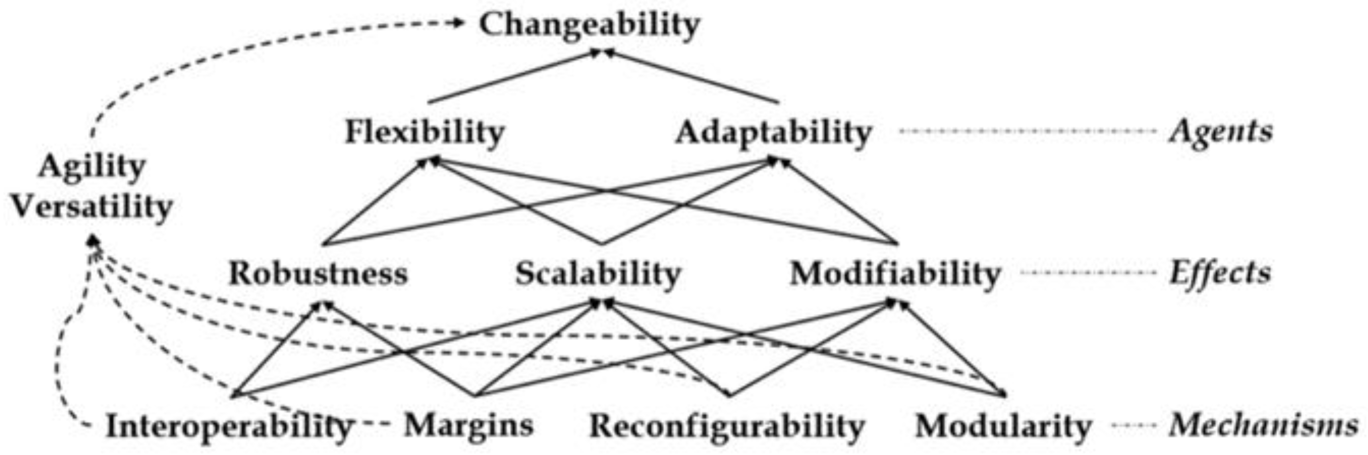
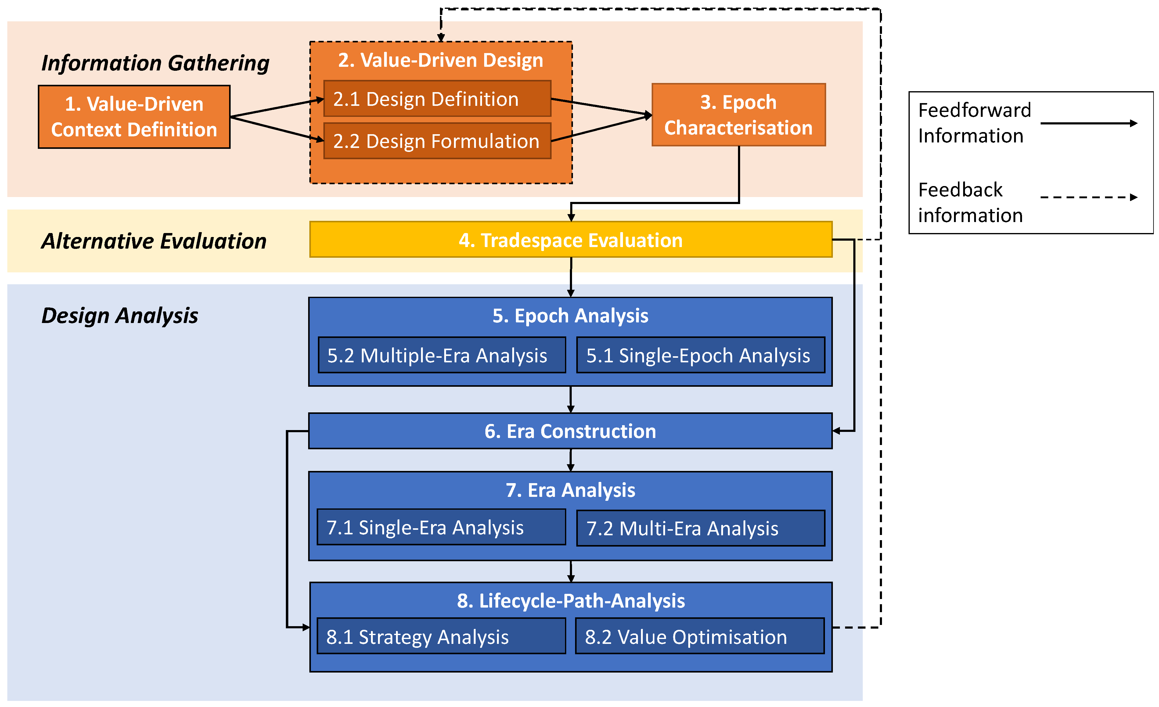
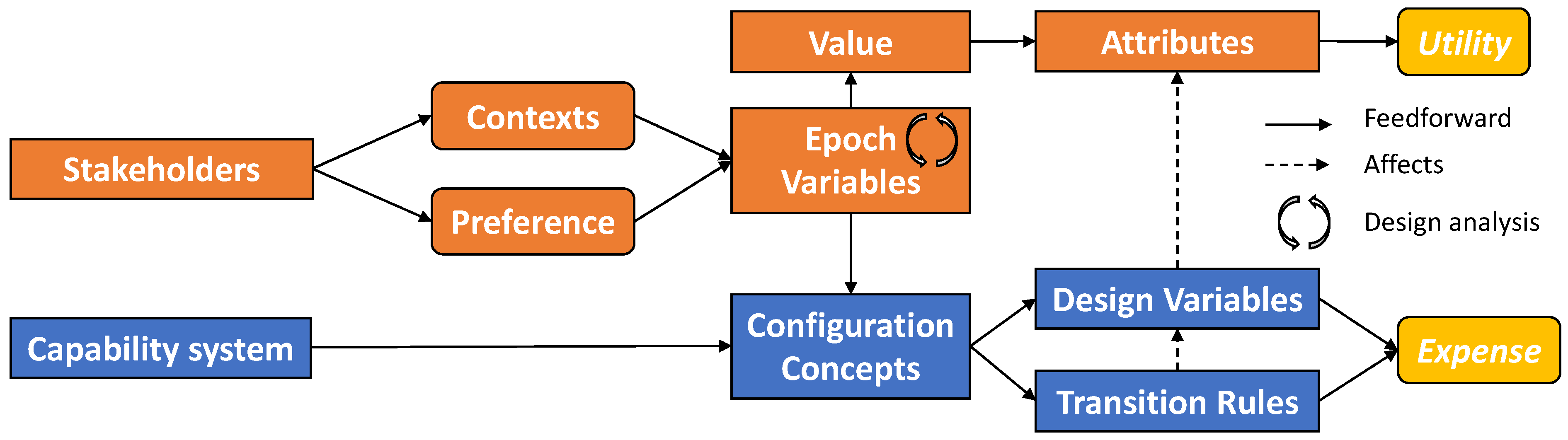
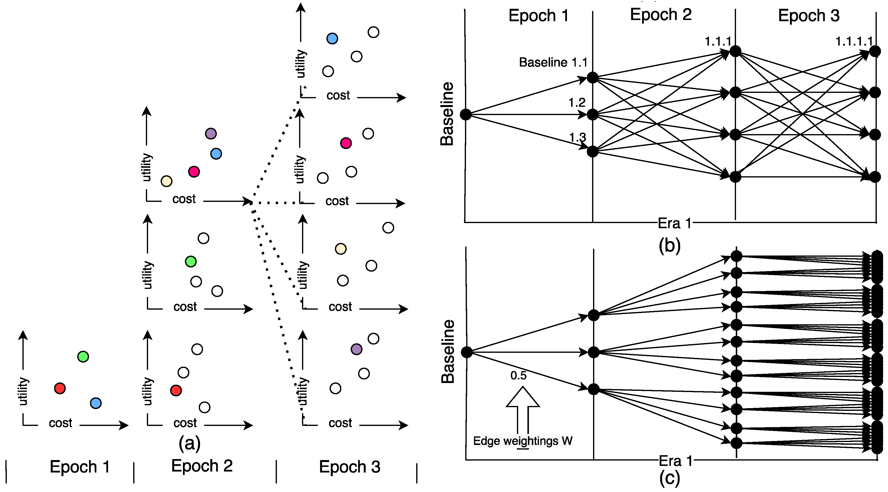
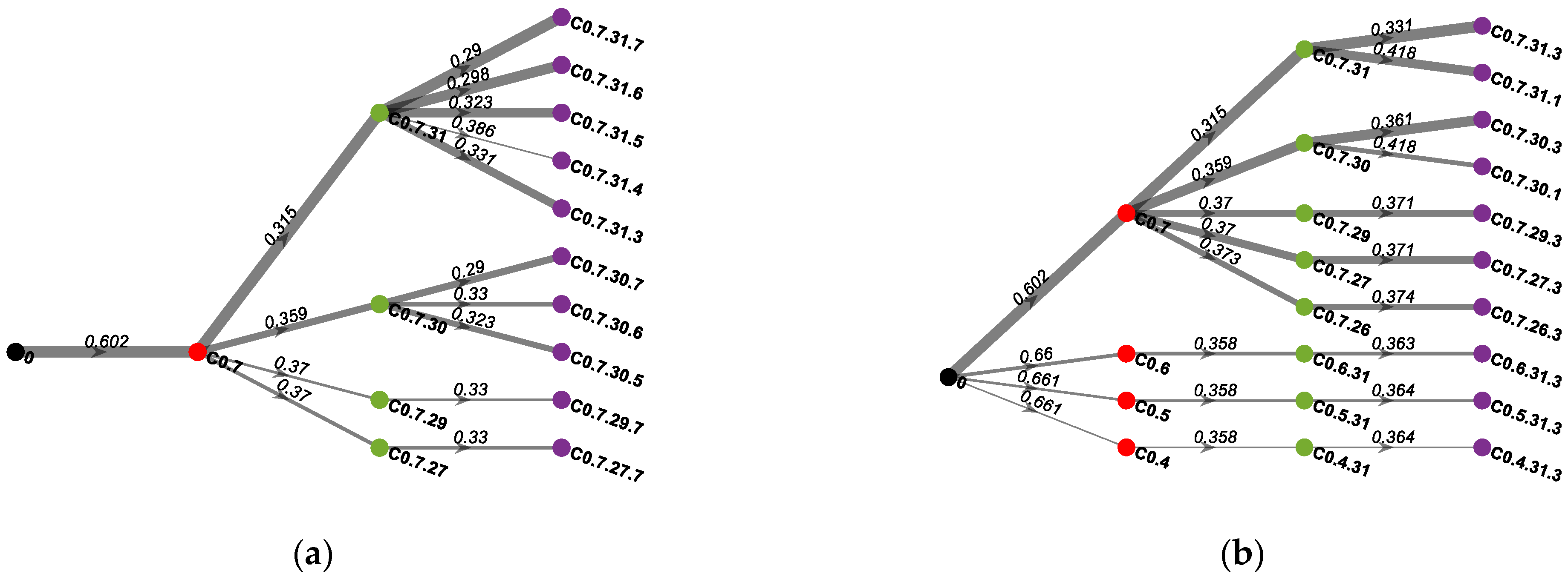
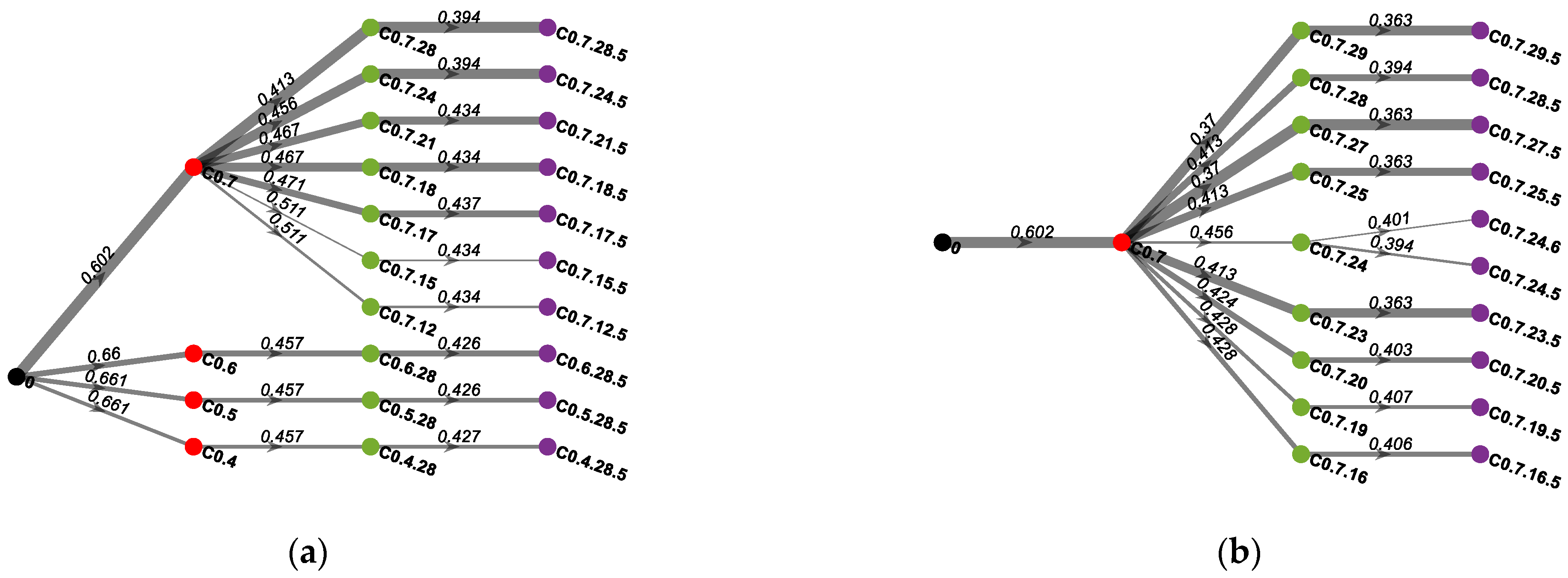
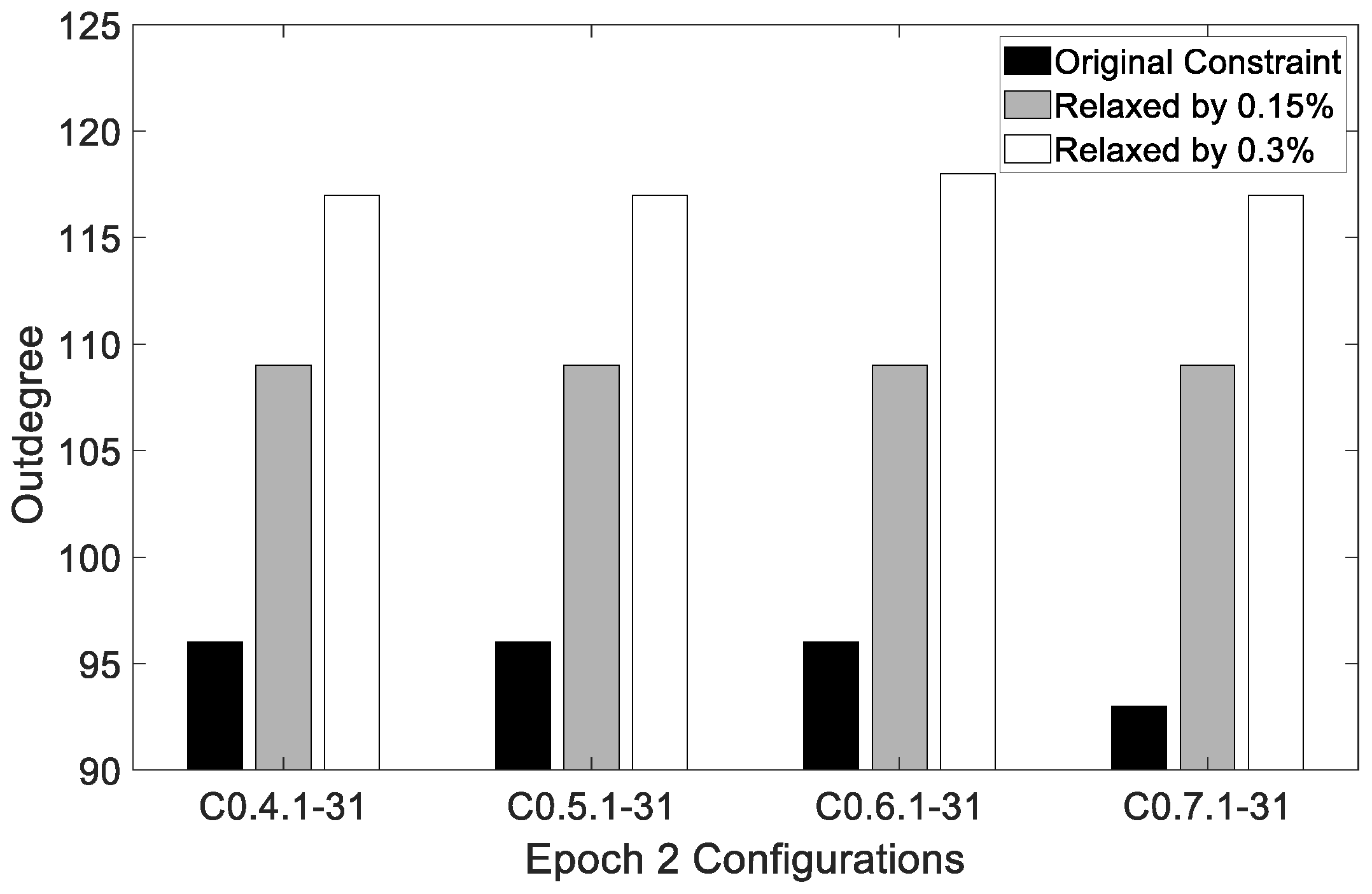
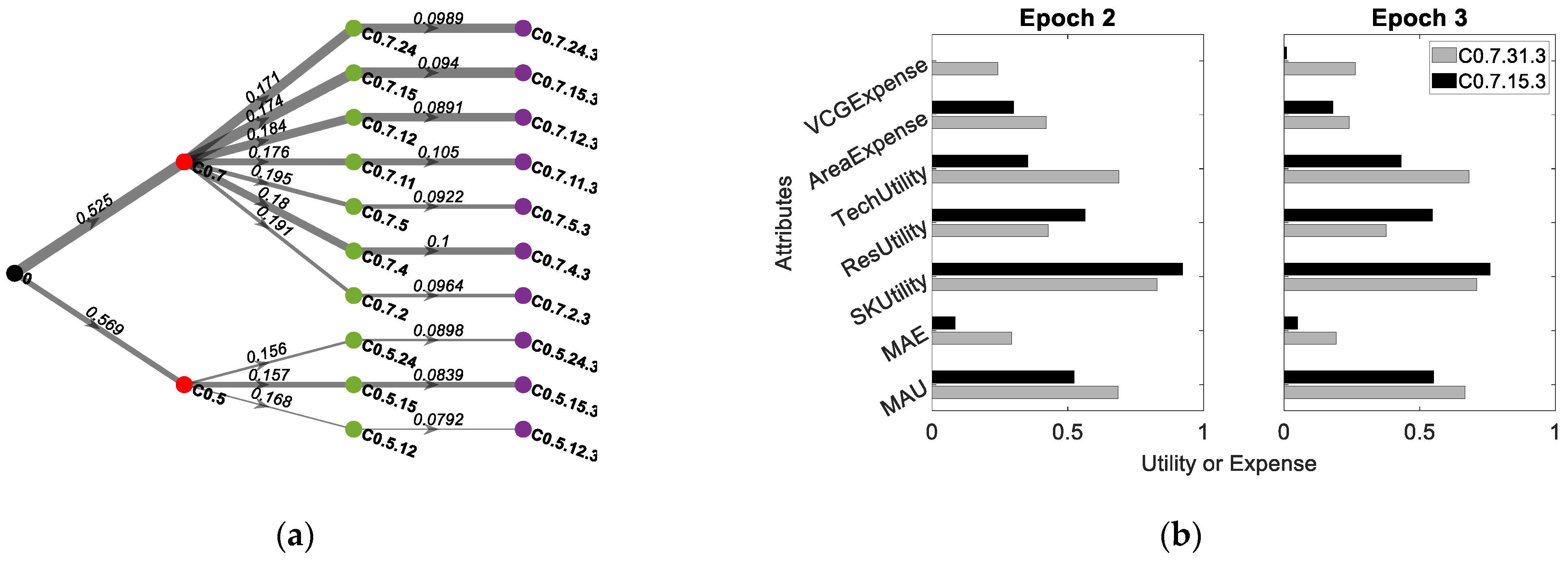
Table 1.
Generic frigate characteristics.
| Characteristic | Value (Units) |
|---|---|
| Mass | 3600 (tons) |
| Length Overall | 118 (m) |
| Beam | 14.8 (m) |
| Draft | 4.35 (m) |
| Max Speed Range | 27 (knots) 6000 (nautical miles) |
| Complement | 179 (officers, sailors, crew) |
Table 2.
Transition rules and their values.
| Transitional Rules | Units | Available (A)/Limit (L) |
|---|---|---|
| Area Margin | m2 | 717 (A) |
| Volume Margin | m3 | 346 (A) |
| Mass Margin | tons | 3800 (L) |
| VCG Margin | m | 6.28 (L) |
Table 3.
Expense and utility attributes and their ranges.
| Utility Attributes (U) | Units | Level Range (X) (Worst–Best) | Weighting (k) |
|---|---|---|---|
| Technological Capability | Nil | 0–1 | 0.7 |
| Seakeeping | Nil | 0–1 | 0.1 |
| Resistance | kN | 6400–1600 | 0.1 |
| Stability (Metacentric Height) | m | 0.6–1.45 | 0.1 |
| Expense Attributes (E) | Units | Level Range (X) (Worst–Best) | Weighting (k) |
| Area Margin Remaining | % | 0–100 | 0.25 |
| Volume Margin Remaining | % | 0–100 | 0.25 |
| Mass Margin Remaining | % | 0–100 | 0.25 |
| VCG Margin Remaining | % | 0–100 | 0.25 |
Table 4.
Design variables and their ranges. “No, Yes” denote a positive or negative value for conducting upgrades, or the addition of the technology described by the variable.
Table 4.
Design variables and their ranges. “No, Yes” denote a positive or negative value for conducting upgrades, or the addition of the technology described by the variable.
| Design Variable (Acronym) | Range (Units) |
|---|---|
| Mass a | 3600–3800 (tons) |
| Length Waterline | 109–110 (m) |
| Draft | 4.4–4.6 (m) |
| Vertical Centre of Gravity (VCG) a | 5.9–6.3 (m) |
| Cruising Speed Profile | 15–19 (kn) |
| Operating Wave- Length + Height | 9–13 (s) + 3–5 (m) |
| Torpedoes (Torp.) a | No, Yes |
| Helicopter (Hel.) a | No, Yes |
| Towed Array (TA) a | No, Yes |
| Radar a | No, Yes |
| Main Gun Ammo (MGA) a | No, Yes |
| Vertical Launch System (VLS) a + Seasparrow Missiles (SSM) a | No, Yes |
| Tactical Data Link (TDL) a | No, Yes |
| Search and Track System (STS) a | No, Yes |
| Automatic Guns (AG) a | No, Yes |
| Harpoon Missiles (HM) a + Launcher (Laun.) a | No, Yes |
a denotes design variables which are path-dependent through epochs.
Table 5.
Epoch Variables and Their Values. b denotes epoch variables which are subject to mass and size growth rates. “No, Yes” denote a positive or negative value for conducting upgrades or additions.
Table 5.
Epoch Variables and Their Values. b denotes epoch variables which are subject to mass and size growth rates. “No, Yes” denote a positive or negative value for conducting upgrades or additions.
| Uncertainty Category | Epoch Variable | Values (Units) |
|---|---|---|
| ASW Capability | Upgrade Torp. b | No, Yes (-) |
| Upgrade Hel. b | No, Yes (-) | |
| Upgrade TA b | No, Yes (-) | |
| AAW Capability | Upgrade Radar b | No, Yes (-) |
| Add VLS + Upgrade SSM b | No, Yes (-) | |
| Upgrade MGA b | No, Yes (-) | |
| Add TDL | No, Yes (-) | |
| Add STS | No, Yes (-) | |
| ASuW Capability | Upgrade Radar b | No, Yes (-) |
| Upgrade AG b | No, Yes (-) | |
| Add Launch. + Upgrade HM b | No, Yes (-) | |
| Operating Condition | Dominant cruise speed | 15, 17, 19 (kn) |
| Operating Environment | Sea State | 3, 4, 5 (-) |
Table 6.
ERA Construction, EVs and Values, Up. = upgrade.
| Epoch 1 ASW | Epoch 2 AAW | Epoch 3 ASuW |
|---|---|---|
| EVs (values) | EVs (values) | EVs (values) |
| Up. Torp. (no, yes) | Up. Radar (no, yes) | Up. Radar (no, yes) |
| Up. Hel. (no, yes) | Add VLS + Up. SSM (no, yes) | Add Launch. + Up. HM (no, yes) |
| Up. TA (no, yes) | Up. MGA (no, yes) | Up. AG (no, yes) |
| Cruise Speed (15) | Add TDL (no, yes) | Cruise speed (19) |
| Sea State (3) | Add STS (no, yes) | Sea State (5) |
| Cruise Speed (17) | ||
| Sea State (4) |
Disclaimer/Publisher’s Note: The statements, opinions and data contained in all publications are solely those of the individual author(s) and contributor(s) and not of MDPI and/or the editor(s). MDPI and/or the editor(s) disclaim responsibility for any injury to people or property resulting from any ideas, methods, instructions or products referred to in the content. |
© 2023 by the authors. Licensee MDPI, Basel, Switzerland. This article is an open access article distributed under the terms and conditions of the Creative Commons Attribution (CC BY) license (https://creativecommons.org/licenses/by/4.0/).
Share and Cite
MDPI and ACS Style
Dwyer, D.; Efatmaneshnik, M. Lifecycle Value Sustainment and Planning Mission Upgrades for Complex Systems: The Case of Warships. Systems 2023, 11, 183. https://doi.org/10.3390/systems11040183
AMA Style
Dwyer D, Efatmaneshnik M. Lifecycle Value Sustainment and Planning Mission Upgrades for Complex Systems: The Case of Warships. Systems. 2023; 11(4):183. https://doi.org/10.3390/systems11040183
Chicago/Turabian StyleDwyer, Dylan, and Mahmoud Efatmaneshnik. 2023. "Lifecycle Value Sustainment and Planning Mission Upgrades for Complex Systems: The Case of Warships" Systems 11, no. 4: 183. https://doi.org/10.3390/systems11040183
Note that from the first issue of 2016, this journal uses article numbers instead of page numbers. See further details here.