

High-Speed Rails and City Innovation System: Empirical Evidence from China


Institute of Social Science Survey, Peking University, Beijing 100871, China
Systems 2023, 11(1), 24; https://doi.org/10.3390/systems11010024
Submission received: 23 November 2022
/
Revised: 26 December 2022
/
Accepted: 1 January 2023
/
Published: 4 January 2023
(This article belongs to the Special Issue Decision Making and Policy Analysis in Transportation Planning)
Abstract
:The rapid development of high-speed rail has markedly shortened the travel time from one city to another. However, the impact of space–time compression brought about by high-speed rail on city innovation has not received sufficient attention. This paper examines the space–time compression phenomenon produced by high-speed railway networks and its impact on city innovation from 2000 to 2019 using a sample of 279 Chinese prefecture-level cities. The empirical results show that there was a strong space–time compression during this period. The development of high-speed rail can promote city innovation. However, the construction of high-speed rail also produces a siphon effect, which accelerates the convergence of innovative elements in cities with stronger innovation capabilities. Nevertheless, it has a negative spillover effect on cities with weaker innovation capabilities. Finally, policy recommendations for promoting the balanced development of city innovation and recommendations for future research are presented.
1. Introduction
The development of cities has become a major engine of regional and national development [1,2]. At present, 54% of the global population lives in cities, and the global urbanization process is accelerating [3]. According to a United Nations report, the proportion of the global urban population is expected to hit a record of 68% by 2050 [4]. Referred to as the soul of a city and its competitiveness, the capability for innovation is the source of a city’s value creation process and the key to its comprehensive competitiveness [5,6,7]. With the rapid advancement of economic globalization and convenient transportation, as well as rapid advances in science and technology, time and space have been compressed and the world has shrunk into a “global village” [8,9]. In this context of space–time compression, cities have become increasingly important in the global system, acting as basic units of direct participation in international economic activities [10,11]. However, because innovation activities in cities are a complex systemic project, they involve time, space, and society. Therefore, studying the city innovation system in the context of space–time compression is of great significance for cultivating the innovation capability and competitiveness of cities.
According to the existing literature, researchers have reached a preliminary consensus on the basic components of the city innovation system [12,13,14]. However, some key factors, such as spatio-temporal context, transport infrastructure, and space–time compression, have not received much attention. The impact of space–time compression caused by transportation development on city innovation is still in a “black box” state. Most of the related studies on space–time compression are qualitative analyses [15,16,17], and they rarely measure space–time compression from a quantitative perspective. Quantitative research on space–time compression and its impact on city innovation is still in its infancy. With the large-scale development of high-speed rail (HSR), the increasing impact of HSR on regional economies has received widespread attention [18,19,20]. The introduction and rapid development of HSR overcomes geographical and spatial barriers and effectively improves city accessibility, resulting in space–time compression [21,22]. Most studies on the impact of HSR on innovation have been analyzed at the national, provincial, and company levels [23,24,25], lacking a level of analysis for cities. The impact of the introduction of HSR can be assessed at different levels (national, provincial, city, or company), but the focus of the assessment is often different at different levels. In fact, due to the heterogeneity of cities, the impact of HSR on city innovation can vary, a fact that has not received attention in the existing studies. To control for heterogeneity between cities, the term “cities” in this study refers to prefecture-level cities in China.
In this study, panel data for 279 Chinese prefecture-level cities from 2000 to 2019 were used to investigate the increasing impact of HSR construction on urban innovation from a space–time compression perspective. The upgrading of transportation infrastructure is an important driver of economic growth; specifically, the advent of HSR has far-reaching effects on traditional transportation patterns, economic development, and technological innovation, so it is of great practical significance to study the impact of high-speed rail on urban innovation. In addition, HSR, similarly to the Internet and airline facilities, has changed the spatiotemporal relationship between cities and regions, as well as people’s travel concepts and lifestyles, bringing new development opportunities for urban innovation. With regard to the current uneven development of scientific research strength between cities and regions, how does the space–time compression brought about by HSR change the space–time pattern of innovation? This is a common concern among various countries.
The academic contributions of this paper are as follows. First, this paper plays an important role in enriching and expanding the existing literature on urban innovation systems. In the study of city innovation systems (CISs), the existing literature has focused on firms [26], industries [27], social innovation [28], dynamic capabilities [29], and networks [30]. However, these studies have ignored the intrinsic interconnectedness of innovation systems among neighboring cities. In this paper, we consider the innovation system among neighboring cities as a whole, i.e., a regional innovation system formed from the merging of intra-city innovation systems and cross-city innovation systems, and an important driving factor of this merger is the construction of HSR. Second, this study contributes to the theory of space–time compression by empirically measuring space–time compression and its impact on urban innovation. Although studies from Harvey [15] and Janelle [31] have elaborated upon the concept of space–time compression, measurements and empirical tests of space–time compression are lacking. The present study fills this knowledge gap. Finally, this paper enriches the study of the consequences of the introduction of HSR. The existing literature has examined the impact of HSR on regional economic development [32] and internal migration [33], but less attention has been paid to urban innovation systems. This paper complements the research on the economic consequences of HSR by linking the introduction of HSR to urban innovation based on an integrated local and neighborhood hierarchy from a holistic system perspective, which is an emerging field that has so far received relatively little attention from scholars.
The paper is structured as follows. The development of China’s HSR and the concept of space–time compression are introduced in Section 2. The theoretical background, literature review, and development of the hypothesis are discussed in Section 3. Information about the data, variables, and methods is reported in Section 4. The empirical results are reported and some robustness checks are provided and discussed in Section 5. The final section concludes the paper.
2. High-Speed Rail in China and Space–Time Compression
HSR is a milestone in the integration of transportation technology and railway modernization. In 2003, the Qinhuangdao–Shenyang passenger-dedicated line was opened. It was China’s first HSR in the true sense, marking the beginning of China’s HSR era. The rapid development and construction of HSR in China has brought great convenience to people’s travel. By the end of 2021, the total operating mileage of HSR in China reached 40,000 km, accounting for about 70% of the world’s HSR network [34]. According to statistics from the National Railway Administration of China, in 2019, electric multiple units (EMUs) carried 2.29 billion passengers, an increase of 14.1% compared to 2018, accounting for 64.1% of railway passenger traffic. In addition, the introduction of HSR has also greatly reduced the space–time distance, improved transport accessibility and economic connections, and accelerated the cross-regional flow of economic factors [35].
Cities with convenient transportation connections tend to be in close proximity to each other, and “space–time compression” occurs in geographic space along the direction of transportation connections. Empirical evidence from China and other countries shows that the development of HSR has facilitated the process of space–time compression [36]. In mainland China, the development of HSR has brought cities closer together, which, in turn, has contributed to space–time compression [18,19,37]. For example, in Taiwan, China, the construction and development of HSR has led to space–time compression with varying uniformity in the geographical areas along its route [38]. The introduction of HSR has reduced the space–time distances between cities in continental Europe [39]. European HSR has compressed time and space by compressing temporal distances and changing relative positions [40]. Similar empirical evidence has also been obtained from Japan [23]. However, there is still a lack of relevant research on the impact of this space–time compression caused by HSR on city innovation.
3. Theoretical Background and Hypothesis Development
With the development of modern transportation and communication technology, people generally have access to a completely different social space and time experience than before [17]. Scholars in different fields have begun to pay more and more attention to exploring the phenomenon of space–time compression caused by the development of transportation and communication technology [31,41]. The advancement of modern technology has led to a “global village” [15]. The theory of space–time compression refers to the shortening of the human travel time between two places due to the progress and development of transportation [42]. Space–time compression has led to the emergence of fluid space [16,43].
To assess the impact of space–time compression, it is necessary to delve into the measurement of the degree of space–time compression. Harvey [15] concept of space–time compression is only used as a framework for analyzing social, cultural, and institutional changes and lacks a measurable approach [44]. The approach based on the average rate of time–space convergence, proposed by Janelle [31], also has limitations. For example, the average rate of time–space convergence has the disadvantage of being unstable and vulnerable to distance. The use of an “isochrone map” is another method [45]. However, it does not fully show the overall pattern of regional multi-node space–time compression. Some scholars, such as Spiekermann and Wegener [39] and Vickerman, et al. [46], have tried to modify and improve the above methods from the perspective of traffic accessibility by plotting time–space maps but have failed to effectively overcome their limitations. A common weakness of these measures is their treatment of travel time as static. Consequently, these measures fail to capture the potential dynamics of social time and social space, which is the core of social-spatial theory [47,48]. Therefore, a breakthrough in the methods of measuring space–time compression is needed to advance the development of spatiotemporal social science.
The theory of “space–time compression” emphasizes the important influence of fast-developing transportation technologies and tools on people’s communication in this modern and fast-paced society. Spatial distance is an important factor that affects interpersonal relationships between two places [17]. As Tobler’s First Law of Geography says, everything is related to everything else, and near things are more related than distant things [49]. The construction of HSR has greatly optimized the original transportation network, shortened the space–time distance, and positively influenced regional economic growth [20,22]. The flow of innovation elements is limited by spatial distance [50]. With the compression of spatial distances, the effectiveness of tacit knowledge dissemination and face-to-face communication gradually increases and the frequency of information exchange increases as well [51]. Innovative entities can acquire more tacit knowledge in face-to-face communication, resulting in better performance in cooperative research and development [52,53] and purchases of technology [54]. These activities have been shown to be significantly and positively correlated with patent citations [55].
Hypothesis 1 (H1).
The introduction of HSR promotes city innovation.
The introduction of HSR leads to time and space compression between cities along the route, which intensifies the innovation competition among these cities. The rapid development of HSR intensifies competition between cities and regions, thereby changing the spatial patterns of cities [37]. The introduction of HSR can facilitate the flow of innovation-related information and innovative talent between cities along the route [19,56]. Qin [57] found that HSR helps to boost economic activities between large cities due to significantly shorter travel times, and it may actually hurt smaller counties along accelerated railway lines. The introduction of HSR exacerbates the imbalance of urban centrality, forming a hierarchical spatial structure with big cities as innovation hubs, but it also impedes local economic growth and innovation in peripheral areas [18]. HSR connections and networks significantly increase the cost of debt by 2.2% for firms that are located in those non-node cities [58]. Innovation and economic growth are inevitably boosted in those regional centers but suppressed in those adjacent and peripheral regions due to the agglomeration effect of transport infrastructure [59,60,61]. With the introduction of HSR, innovation elements, such as talent, information, and funding, are more likely to flow to cities with stronger innovation capabilities, which will have a negative impact on the innovation capabilities of cities with relatively weaker innovation capabilities. Therefore, the introduction of HSR will intensify inter-city competition and lead to negative spillover effects in terms of innovation.
Hypothesis 2 (H2).
There is a negative spillover effect of inter-city innovation.
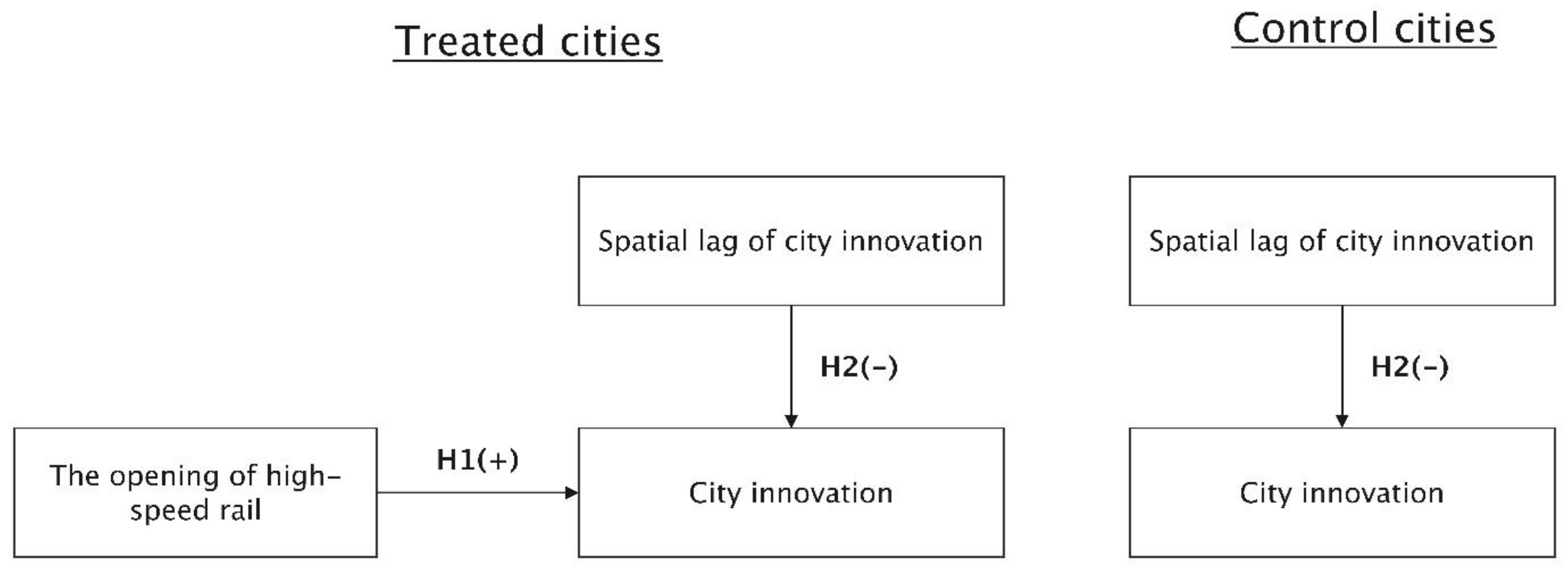
The analytical framework for understanding the impact mechanism of HSR on city innovation is illustrated in Figure 1. The test of the so-called spatial spillover effect proposed in the abovementioned Hypothesis 2 was realized empirically by means of a spatial lag term [62,63,64]. This analysis framework was constructed using the spatial difference-in-differences method, and its purpose was to handle three different treatment effects that existed at the same time in the process of natural experiments: the treatment effect due to the introduction of HSR, the spillover effect within the treated cities, and the spillover effect on the control cities. In other words, in terms of innovation, there is a spatial dependence between cities along the HSR route [21]. These cities interact strategically with each other, rather than independently of each other [62,63]. In evaluating the impact and effect of HSR on urban innovation, it is necessary to include and examine the potential impact of inter-city spatial dependence.
4. Data, Variables, and Empirical Strategies
4.1. Data
The research object of this study was China’s prefecture-level cities, with a total sample consisting of 279 prefecture-level cities. The study period spanned two decades from 2000 to 2019. Therefore, the total number of observations was 5580. Data were obtained from the statistical yearbooks of Chinese cities over these years. The key data in this paper were the data concerning the introduction of HSR, which was manually compiled from the official website of the Chinese National Railway Administration. Panel data for 279 prefecture-level cities across the country from 2000 to 2019 were used in this study as balanced data.
4.2. Variables and Measurement
4.2.1. Dependent Variables
Generally, inventions refer to new technical solutions, breakthrough ideas, or new processes proposed for products, methods, or improvements [65]. Inventions, together with utility models and designs, constitute the object of protection under China’s patent law [66]. Due to their high technological value, invention patents can be used more objectively to measure a city’s innovation capability and to evaluate the technological competitiveness of a city more accurately [67]. Therefore, in this study we used the number of invention patents granted (NIP) as the dependent variable.
4.2.2. Independent Variables
The location of the HSR network was determined based on information from the National Development and Reform Commission and the railway company, according to a comprehensive plan. The local government has little influence on its location. Therefore, the introduction of HSR can be used as a treatment in a quasi-natural experiment. To capture the impact of the introduction of HSR on the changes in city innovation output, cities that introduced HSR between 2000 and 2019 were selected as the treatment group in this paper, and cities that did not introduce HSR during the same period were selected as the control group. The treatment group included a total of 190 cities, all of which introduced HSR before 2020. The remaining 89 cities belong to the control group. In this study, in order to test the impact of the introduction of HSR on the city’s innovation capability, we introduced an independent variable, . Here, is a combined and newly created dummy variable, and it is the product of the dummy variable of the group and the dummy variable of the introduction of HSR is calculated as follows: , where is a dummy variable that is used to distinguish the experimental group from the control group: if they are cities in the treatment group (cities where HSR was introduced), and if they are not cities in the treatment group; is a dummy variable used to reflect the local patent policy: if they are cities in the year when HSR was opened and every year thereafter, and in the previous year; and are the mean values of those two dummy variables.
In addition to the abovementioned core independent variable, several other independent variables were included in this study. The number of employees in each city in the comprehensive scientific and research technical services (NES) industry was used to measure the development of urban technical services, expressed per 10,000 people. Scientific expenditure (SE) was used to measure the city’s investment in science and technology, expressed in CNY 100 million. The number of college students per 10,000 people (NCS) was used to measure the city’s stock of human resources. The number of ordinary colleges and universities (NCU) was used to measure the degree of development of higher education in the city. The number of R&D personnel (NRD) was used to measure the city’s R&D human resources, expressed in number of people. The export value of goods (EVG) was used to measure the city’s foreign trade export capacity, expressed in CNY 100 million. The number of foreign-invested enterprises (NFI) was used to measure the city’s ability to attract foreign investment. The total industrial output value of domestic-funded enterprises (TVD) was used to measure the city’s own industrial strength, expressed in CNY 100 million. Per capita GDP (PGDP) was used as a measure of a city’s overall economic strength, expressed in CNY. The sample size and descriptive statistics of these variables are reported in Table 1 below.
4.3. Methods
4.3.1. Standard Deviation Ellipse Method
D. Welty Lefever’s famous standard deviation ellipse (SDE) method was used to identify the spatial center of gravity of each city’s innovation [68]. This method has been widely used in innovation research [69,70]. This method analyzes the spatial distribution of the target variable by calculating the standard deviation ellipse of the target variable and its center of gravity [71,72].
4.3.2. Difference-in-Differences Method
The so-called difference-in-differences model is widely used in quasi-experimental studies [73,74]. However, the traditional difference-in-differences model involves the premise that the observed samples are independent of each other [75]. In this study, we used the difference-in-differences model. Since the introduction of HSR occurred in the form of sequential events, in the experimental group we could distinguish between pre- and post-events, whereas in the control group we could not. In addition, in this study we assumed that the studied cities were not independent of each other but performed strategic interactions that led to the spillover effects of innovation [76]. The spatial difference-in-differences (SDiD) model has been proven in previous studies to deal effectively with the abovementioned problems [77,78]. Therefore, in this study, we drew on the work of Heckert [75] and Gu [79] and modified the difference-in-differences equation as follows:
The model can be expressed as follows:
where is the constructed spatial weight matrix. Traditionally, the spatial weight matrix is defined by t and the inverse distance is constructed as follows: , where is the spatial distance from observation point to observation point . What is used here is not the geographical distance between cities but the innovation distance between cities. In calculating the innovation distance, the difference in the number of patents granted between cities is used. The calculation formula is as follows: . Here, and represent the average annual number of patents granted from 2010 to 2019 for city i and city j, respectively.
In this study, our model was focused on the regression coefficient and the regression coefficient . The former reflects the changes in the innovation ability of cities before and after the introduction of HSR in cities with HSR and compares the differences in the innovation capabilities of cities without HSR. The latter reflects the spatial spillover effect of inter-city innovation. According to Hypothesis 1, in Formula (1) should be significant and positive. According to spatial econometrics, is usually used to identify and test the spatial spillover effect [80,81]. If is statistically significant and negative, a negative spatial spillover effect exists [69,70]. According to Hypothesis 2, in Formula (1) should be significant and negative.
5. Results
5.1. Space–Time Compression Process Analysis
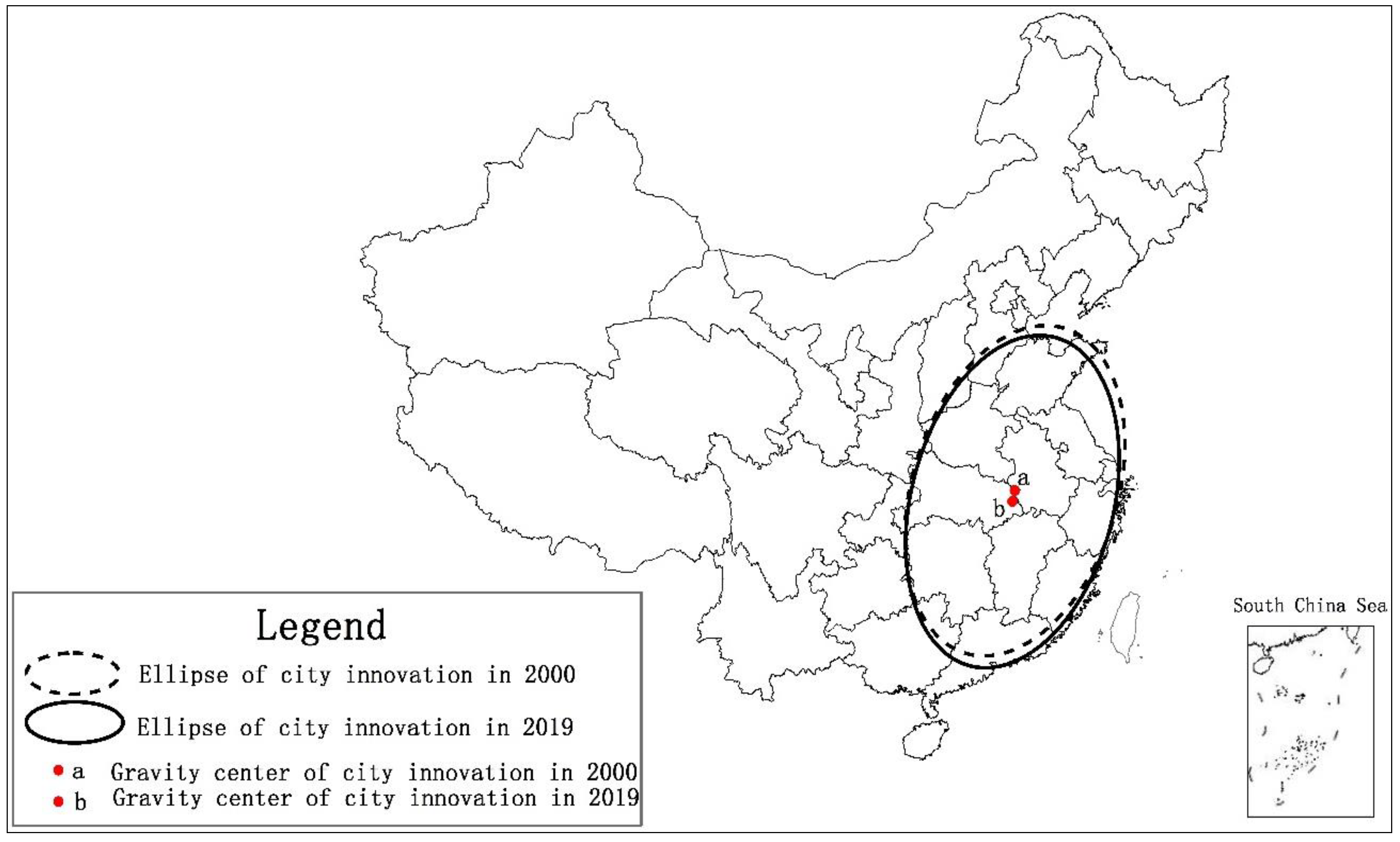
Space–time compression is a very abstract concept. Here, the SDE method was used to intuitively reflect the process of space–time compression. Figure 2 shows the ellipses created by SDE and the centers of gravity, calculated based on the number of invention patents of 279 prefecture-level cities in 2010 and 2019. As shown in Figure 2 below, from 2010 to 2019, the spatial center of gravity of city innovation moved to the southwest. The ellipse also showed a similar trajectory of movement. It can be seen that the introduction of HSR changed the spatial pattern of urban innovation, causing the center of gravity to move towards the southwest.
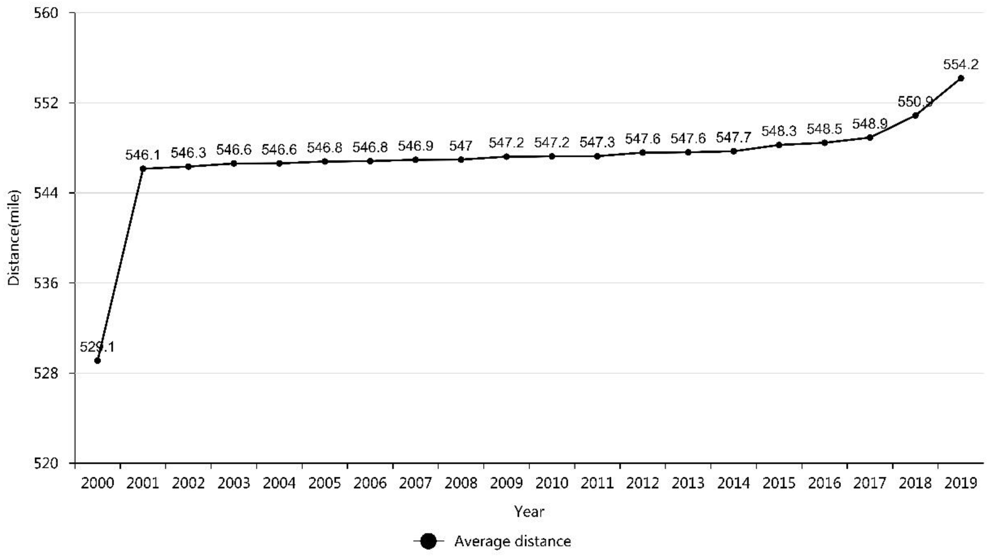
However, according to Figure 2, the process of space–time compression cannot be tested directly. The traditional measurement of space–time compression is also static and partial [31,40,46]. It is a challenging task to comprehensively measure the compression process of the social space–time pattern. To test the social space–time compression process, the following steps are required: first, calculate the center of gravity of the city’s innovation for each year; second, calculate the geographical distance from the spatial center of gravity to each city in each year; third, calculate the average distance from the spatial center of gravity to each city in each year. Finally, based on the variation in this average distance over time in a year, the presence of space–time compression is judged and tested. This principle is similar to compressing a plastic cup filled with water by hand. The greater the compression, the more water overflows from the plastic cup. Therefore, the degree of compression of a plastic cup can be measured by measuring the amount of overflowing water, which is the reverse side of plastic cup compression. This is the method of reverse measurement and testing. This analogy of the plastic cup is actually consistent with Newton and Kant’s argument that space is a container [82]. Following the same principle here, we can measure the degree of space–time compression by measuring the change in the average distance from the spatial center of gravity of city innovation to each city. This average distance actually measures the spillover of knowledge from the core to the periphery of city innovation, which is the reverse side of the physical space–time compression due to the availability of convenient transportation. This average distance becomes increasingly larger over time, indicating increasingly stronger space–time compression. The average distance from the spatial center of city innovation to each city is summarized in Figure 3.
As shown in Figure 3, the average distance showed a continuous upward trend since 2000. This indicates that with the successive introduction of HSR and the increase in the mileage of HSR, the compressibility of time and space was strengthened. After 2001, the average distance showed a steady and continuous upward trend, whereas, after 2016, the growth trend of the average distance was markedly accelerated. This shows that after 2016, there was a certain accumulation of HSR mileage and a leap from quantitative to qualitative change, which led to the acceleration and intensification of space–time compression. The impact of space–time compression on regional urban innovation systems is also demonstrated graphically in Figure 4.
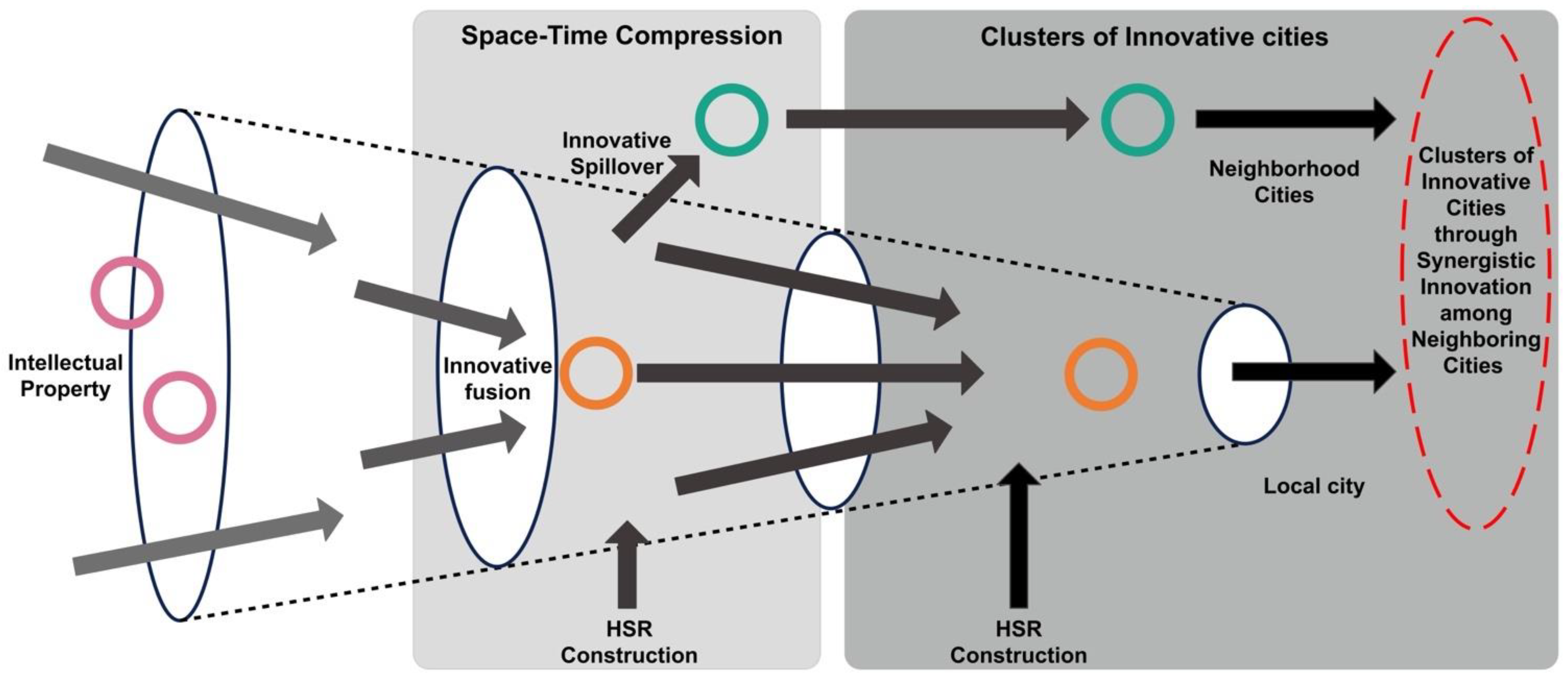
In Figure 4, the small circles represent the innovation elements of the city and the ellipses represent the innovation system within the city. The red-dashed ellipse represents a larger picture of the overall innovation system, including the innovation system of the city under study and the neighboring cities. With the advancement of space–time compression brought about by the construction of HSR, the innovation elements of the city are rapidly fissioned and continue to spill outward, thus influencing the innovation of other neighboring cities. Space–time compression leads to closer spatial and temporal distances between neighboring cities, reducing the cost of collaborative innovation between cities and creating a clustering effect of innovative cities. It is evident that space–time compression affects not only intra-city innovation systems but also cross-city innovation systems. Therefore, it is necessary to have a larger systematic view of urban innovation systems that can include both local and nearby urban innovation systems. This is a holistic, big-picture systematic view.
Furthermore, it must be noted that this is still a dynamic system. The space–time compression brought about by the introduction and construction of high-speed rail leads to a fusion of innovation systems within cities, allowing urban innovation to focus more on technological areas related to core competencies. At the same time, space–time compression also leads to the fission of urban innovation systems, and some innovation elements spill over to neighboring cities, leading to the formation of regional innovation synergy. As demonstrated in Figure 4, this dynamic mechanism is an iterative process, leading to the continuous fusion and fission of urban innovation systems and eventually to the organic integration of intra-city and cross-city innovation systems and the emergence of innovative urban agglomerations.
5.2. Empirical Results
Figure 3 intuitively illustrates the space–time compression process that occurs in city innovation. However, the question of whether this space–time compression is driven by the introduction and development of HSR requires further research and testing. Here, this was tested empirically by means of the SDiD method. The empirical results are reported in Table 2. Model 1 in Table 2 is the model with fixed effects, whereas Models 2, 3, and 4 in Table 2 are models with random effects. In Model 2, only the year was fixed. In Model 3, the year and city were fixed. In Model 4, the year, city, and province were fixed. The Hausman test was insignificant, indicating that the model with random effects here was much better than the model with fixed effects. The empirical results are reported and summarized in Table 2.
As shown in Table 2, the coefficients of the key variable (DID) were significant in all four models. Thus, Hypothesis 1 was confirmed. The number of patented inventions in cities increased with the introduction of HSR. That is to say, the introduction of HSR enhanced the innovation capability of cities. This finding is obviously consistent with the research results of Agrawal, et al. [83] regarding highway construction, which showed that transport infrastructure may lead to an increase in regional patenting. The introduction of HSR facilitated the flow of talent between cities along the route, thereby increasing the likelihood that innovators in different cities would engage in collaborative innovation to improve their innovation capabilities [53]. With the introduction of HSR, researchers often use HSR instead of flying for intercity transportation, which reduces the cost of transportation between cities, and this decrease in transportation cost has a pivotal role in promoting the production and reconstruction of scientific knowledge [84]. HSR certainly facilitates face-to-face communication among scientists in different cities, which is considered to be one of the most important and lasting drivers of knowledge diffusion and innovation [85]. These are driving forces of urban innovation due to the space–time compression brought about by the introduction of HSR.
Distance is a natural measure of information asymmetry and a natural factor that hinders the diffusion of innovation [50,86]. Although the geographical location cannot be changed, the development of HSR has greatly reduced city accessibility times through space–time compression and has helped to promote city innovation. This is predicted by the theory of space–time compression [17,31,87]. In this regard, Drolc, et al. [87] once urged researchers to take the effects of time and space seriously. However, space–time compression may also be a double-edged sword. Although space–time compression can have a positive effect on innovation, it can also introduce some negative effects. Harvey [15], a proponent of the concept of space–time compression, had a clear understanding of this concept and criticized the many drawbacks brought about by space–time compression for society [44]. Therefore, the compression of time and space needs to be viewed dialectically.
The possible impact of space–time compression caused by HSR on city innovation also needs to be viewed dialectically. As can be seen in Table 2, the regression coefficients of the spatial lag term in all four models were significant and negative. Thus, Hypothesis 2 was confirmed. In other words, there was a negative spillover effect of inter-city innovation. The introduction of HSR has promoted the process of regional integration [37]. The innovation gradient formed by the difference in innovation levels between regional central cities and peripheral cities tends to cause the transfer of innovative elements, such as human capital, transportation conditions, funds, and information from peripheral cities to central cities [18,19,56]. As a result, the innovative development of central cities inhibits the innovative development of peripheral cities and ultimately enhances the polarization of regional innovation [59,60,61]. In other words, this has a siphon effect on surrounding cities or cities with gaps in their innovation capabilities, thus inhibiting the improvement of innovation levels in other cities [58]. The space–time compression caused by the introduction of HSR is likely to lead to a polarization of “the strongest and the weakest” in urban innovation. The so-called Matthew effect in city innovation is not necessarily good for regional innovation and development [88].
In addition, in this study we found that the number of employees in scientific technological research and the integrated technical services industry, scientific expenditure, the number of college students per 10,000 people, the number of R&D personnel, and the export value of goods contributed to promoting city innovation. However, the number of ordinary colleges and universities had a negative and significant impact on city innovation. The number of foreign-invested enterprises, the gross industrial output value of domestic-funded enterprises, and the impact of GDP per capita on city innovation were not significant.
5.3. Placebo Test
To test the validity of the difference-in-differences model, placebo tests are often conducted, using false treatment times rather than real treatment times. Here, two false HSR introduction times were constructed, one with the introduction of HSR one year in advance and the other with the introduction of HSR one year later. According to the two false HSR introduction times, the regression and simulation of the difference-in-differences models were carried out according to Formula (1). In the case of both false HSR introduction time models, the regression coefficients of DID were significant, which showed that the introduction of HSR was not a factor leading to increased urban innovation but merely a proxy variable for other factors reflecting inter-city gaps. In the case of both false HSR introduction time models, one of the regression coefficients of DID was not significant, which showed that the introduction of HSR was a factor contributing to the increase in city innovation. In other words, the improvement in city innovation capabilities could be attributed to the introduction of HSR. These empirical results are reported in Table 3.
According to Models 5 and 6 in Table 3, the regression coefficient of DID was not significant if the introduction time of HSR was delayed by one year. This indicates that the artificial delay in the introduction of the HSR by one year did not affect city innovation, and that the variable of HSR introduction time was not a proxy variable for other factors. In other words, it is reasonable to attribute the improvement of city innovation capabilities to the introduction of HSR.
5.4. Robustness Test: Spatial Error
Robustness testing of the spatial difference-in-differences model needed to be carried out in relation to multiple aspects. One of the most important aspects is to see if the empirical results would change if the settings of the spatial model were to change. The empirical results in Table 2 were obtained based on the spatial lag model. Unlike the previous method, the spatial error model was used here to test whether these results were still valid. In particular, this was achieved by removing the spatial lag term from Formula (1) and then assuming that the error term had a spatial effect: . The empirical results are summarized in Table 4, where Model 11 and Model 12 are placebo tests.
Comparing the empirical results of Model 9 and Model 10 in Table 4 with those of Models 1 and 4 in Table 2, they are essentially the same. In these four models, it is clear that the coefficients of DID are all significantly positive. In addition, the values in Table 2 are all significantly negative. Similarly, the values in Table 4 are consistently significantly negative. This consistency shows that the negative spatial spillover effect of urban innovation was universal. Based on the placebo test, the empirical results of Model 11 and Model 12 in Table 4 were consistent with those of Models 5 and 6 in Table 3, and this indicates that the findings of this study were robust.
5.5. Robustness Tests: Different Spatial Weight Matrices
The test of the robustness of the SDiD model also includes the investigation of whether the empirical results would change as a result of changes in the spatial weight matrix. The spatial distance, in the previous part of this paper, was defined as the gap in the average annual number of city patents granted. Next, the spatial distance was defined as the gap in the average annual number of city patents filed. The empirical results are reported in Table 5, and the detailed empirical results are summarized in Appendix A.
The results of Models 13 and 14 in Table 5 are consistent with those of Models 1 and 4 in Table 2. Based on the placebo test, the results of Models 15 and 16 in Table 5 are consistent with those of Models 5 and 6 in Table 3. The empirical results were similar in that spatial distance could also be defined in terms of the gap in the city’s annual average GDP per capita. The empirical results are summarized in Table 6, and the detailed empirical results are reported in Appendix B.
It can be seen that despite the change in the definition of spatial distance, the results of this study did not change significantly. In other words, the adjustment and changing of the spatial weight matrix did not affect the results of this study, which further illustrates the robustness of the results of this study. Regarding endogeneity problems, as shown in the tests presented above, various types of control variables and fixed-effects models were adopted to address the potential problem of omitted variables. These treatments have controlled the endogeneity problem to some extent.
6. Conclusions
In this paper, the introduction of HSR in China was used as a treatment in a quasi-natural experiment and panel data from 279 prefecture-level cities from 2000 to 2019 was investigated to empirically test the city innovation hypothesis in relation to transportation improvement from the perspective of space–time compression. In this study, we adopted an inverse measurement method to measure physical space–time compression by calculating the average spatial distance from each city’s innovation spatial center to each city. The average distance was found to increase year by year, which implies that the production of HSR networks led to physical space–time compression between cities and also led to an overflow of city innovation. This study also showed that the introduction of HSR was beneficial to face-to-face communication between people, which promoted the dissemination of “soft information”, accelerated knowledge spillover, and was able to significantly improve the level of city innovation. However, the introduction of HSR could also lead to the transfer of innovation factors from cities with weaker innovation capabilities to cities with stronger innovation capabilities, resulting in a negative spillover effect. As a policy implication, the results of this paper suggest that the construction of HSR networks within city agglomerations should be strengthened to form an innovative development space, with city agglomerations as the mainstay of this approach. Central cities have already been connected to the national high-speed railway network. The government should make full use of this advantage to further promote the ability of central cities to radiate and facilitate the development of small- and medium-sized cities with weak innovation capabilities.
However, this study also has some limitations. For example, the samples studied were all prefecture-level cities, excluding smaller county-level cities; the measurement indicators of city innovation were relatively simple and singular; and international comparative studies were lacking. These are some possible directions for future research. Before concluding this paper, it is necessary to emphasize the difference between space–time compression and spacetime compression. Spacetime is a concept related to time and space in quantum physics [89]. However, this concept was gradually introduced into the social sciences [90]. Currently, no research has been published on how to distinguish the difference between space–time compression and spacetime compression and how to evaluate the impact of spacetime compression. This is also an important direction for future research.
Funding
This research was funded by the Social Science Foundation of China grant number 17BSH122 And The APC was funded by the Social Science Foundation of China.
Data Availability Statement
The data presented in this study are available on request from the corresponding author.
Acknowledgments
The authors gratefully acknowledge the Social Science Foundation of China (17BSH122) for the support provided to this research.
Conflicts of Interest
The authors declare no conflict of interest.
Appendix A

Table A1.
Empirical results of robustness tests of another measure of innovation distance.
| NIP | Placebo Test: One Year after | |||
|---|---|---|---|---|
| Model 13 Fixed-Effects | Model 14 Random-Effects | Model 15 Fixed-Effects | Model 16 Random-Effects | |
| DID | 229.241 **(2.07) | 212.685 *(1.93) | 104.648(0.86) | 107.879(0.89) |
| NES | 193.138 ***(2.78) | 298.423 ***(4.62) | 190.205 ***(2.74) | 295.661 ***(4.57) |
| SE | 5.168 ***(6.11) | 5.292 ***(6.28) | 5.135 ***(6.07) | 5.266 ***(6.24) |
| NCS | 0.253 **(2.29) | 0.274 ***(2.5) | 0.255 **(2.3) | 0.274 **(2.5) |
| NCU | −37.009 ***(−10.63) | −32.779 ***(−9.45) | −35.962 ***(−10.43) | −31.814 ***(−9.26) |
| NRD | 0.004(0.87) | 0.02 ***(5.61) | 0.004(0.92) | 0.02 ***(5.65) |
| EVG | 0.47 *(1.85) | 0.958 ***(12.92) | 0.468 *(1.84) | 0.954 ***(12.88) |
| NFI | −0.084(−0.69) | −0.079(−0.66) | −0.075(−0.6) | −0.072(−0.6) |
| TVD | −0.004(−0.35) | −0.014(−1.25) | −0.003(−0.25) | −0.013(−1.16) |
| PGDP | −0.001(−1.42) | −0.001(−1.4) | −0.001(−1.43) | −0.001(−1.42) |
| _cons | 5622.767 ***(10.2) | 5607.706 ***(10.18) | ||
| −4.717 ***(−16.08) | −2.726 ***(−13.74) | −4.715 ***(−16.08) | −2.722 ***(−13.74) | |
| Sigma_u | 1127.713 | 1126.325 | ||
| Sigma_e | 715.213 | 718.57 | 715.451 | 718.808 |
| Province FE | YES | YES | YES | YES |
| City FE | YES | YES | YES | YES |
| Year FE | YES | YES | YES | YES |
| Hausman Test | 356.45 *** | −522.67 *** | ||
| Log likelihood | −42,350 | −45,160 | −42,350 | −45,160 |
| Wald χ2 | 464.86 *** | 1365.58 *** | 461.09 *** | 1365.02 *** |
| Pseudo R2 | 0.659 | 0.702 | 0.665 | 0.7 |
| Wald test of spatial terms | 258.48 *** | 188.89 *** | 258.43 *** | 188.8 *** |
Note: *, **, and *** indicate statistical significance at 0.1, 0.05, and 0.01.
Appendix B
Table A2.
Empirical results of robustness tests of economic distance.
| NIP | Placebo Test: One Year after | |||
|---|---|---|---|---|
| Model 17 Fixed-Effects | Model 18 Random-Effects | Model 19 Fixed-Effects | Model 20 Random-Effects | |
| DID | 217.778 *(1.93) | 185.077 *(1.66) | 98.356(0.73) | 78.848(0.65) |
| NES | 183.04 ***(2.6) | 331.962 ***(5.24) | 180.211 ***(2.56) | 329.595 ***(5.43) |
| SE | 5.12 ***(5.64) | 4.877 ***(5.46) | 5.102 ***(5.61) | 4.857 **(2.48) |
| NCS | 0.27 **(2.37) | 0.327 ***(2.94) | 0.272 **(2.36) | 0.328 ***(2.94) |
| NCU | −38.039 ***(−10.63) | −30.517 ***(−8.61) | −37.114 ***(−10.46) | −29.711 ***(−8.45) |
| NRD | 0.008 **(1.97) | 0.027 ***(7.89) | 0.009 **(2.01) | 0.027 ***(7.93) |
| EVG | 0.664 **(2.57) | 0.654 ***(10.03) | 0.663 **(2.56) | 0.651 ***(9.99) |
| NFI | −0.068(−0.52) | −0.041(−0.32) | −0.058(−0.44) | −0.035(−0.27) |
| TVD | −0.013(−1.17) | −0.016(−1.48) | −0.012(−1.1) | −0.016(−1.41) |
| PGDP | −0.001(−0.95) | −0.001(−0.69) | −0.001(−1.01) | −0.001(−0.74) |
| _cons | −225.333(−0.78) | −232.287(−0.81) | ||
| −2.867 ***(−18.44) | −0.985 ***(−6.68) | −2.867 ***(−18.42) | −0.985 ***(−6.68) | |
| Sigma_u | 930.796 | 929.433 | ||
| Sigma_e | 720.044 | 724.012 | 720.261 | 724.226 |
| Province FE | YES | YES | YES | YES |
| City FE | YES | YES | YES | YES |
| Year FE | YES | YES | YES | YES |
| Hausman Test | 379.35 *** | 358.68 *** | ||
| Log likelihood | −42,420 | −45,160 | −42,420 | −45,160 |
| Wald χ2 | 940.66 *** | 1744.32 *** | 937.02 *** | 1745.74 *** |
| Pseudo R2 | 0.501 | 0.765 | 0.506 | 0.765 |
| Wald test of spatial terms | 339.87 *** | 44.61 *** | 339.28 *** | 44.64 *** |
Note: *, **, and *** indicate statistical significance at 0.1, 0.05, and 0.01.
References
- Liu, Y.; Zhang, X.; Pan, X.; Ma, X.; Tang, M. The spatial integration and coordinated industrial development of urban agglomerations in the Yangtze River Economic Belt, China. Cities 2020, 104, 102801. [Google Scholar] [CrossRef]
- Comunian, R. Rethinking the Creative City: The Role of Complexity, Networks and Interactions in the Urban Creative Economy. Urban Stud. 2015, 48, 1157–1179. [Google Scholar] [CrossRef]
- Ni, P.; Kamiya, M.; Shen, L.; Gong, W.; Xu, H. Reviews of Global Urban Competitiveness 2017–2018 Driving Force, Agglomeration, Connectivity and the New Global City. In House Prices: Changing the City World; Ni, P., Kamiya, M., Wang, H., Eds.; Springer: Clam, Switzerland, 2019; pp. 49–131. [Google Scholar]
- UN. The 2018 Revision of the World Urbanization Prospects; The Population Division of the United Nations Department of Economic and Social Affairs (UN DESA): New York, NY, USA, 2018. [Google Scholar]
- Feldman, M.P.; Audretsch, D.B. Innovation in cities: Science-based diversity, specialization and localized competition. Eur. Econ. Rev. 1999, 43, 409–429. [Google Scholar] [CrossRef]
- Acs, Z.J. Innovation and the Growth of Cities. Contrib. Econ. Anal. 2010, 266, 635–658. [Google Scholar]
- Visvizi, A.; Lytras, M.; Damiani, E.; Mathkour, H. Policy making for smart cities: Innovation and social inclusive economic growth for sustainability. J. Sci. Technol. Policy Manag. 2018, 9, 126–133. [Google Scholar] [CrossRef] [Green Version]
- Forman, C.; Goldfarb, A.; Greenstein, S. How did location affect adoption of the commercial Internet? Global village vs. urban leadership—ScienceDirect. J. Urban Econ. 2005, 58, 389–420. [Google Scholar] [CrossRef]
- Bedir, M.; Hilgefort, J. The global village. Archit. Rev. 2019, 244, 24–27. [Google Scholar]
- Acuto, M.; Leffel, B. Understanding the global ecosystem of city networks. Urban Stud. 2021, 58, 1758–1774. [Google Scholar] [CrossRef]
- Jenkins, P.; Wilkinson, P. Assessing the Growing Impact of the Global Economy on Urban Development in Southern African Cities: Case Studies in Maputo and Cape Town. Cities 2002, 19, 33–47. [Google Scholar] [CrossRef]
- Dvir, R.; Pasher, E. Innovation engines for knowledge cities: An innovation ecology perspective. J. Knowl. Manag. 2004, 8, 16–27. [Google Scholar] [CrossRef] [Green Version]
- Yao, L.; Li, J.; Li, J. Urban innovation and intercity patent collaboration: A network analysis of China’s national innovation system. Technol. Forecast. Soc. Chang. 2020, 160, 120185. [Google Scholar] [CrossRef]
- Boikova, M.; Ilyina, I.; Salazkin, M. Urban Futures: Cities as Agents of Globalization and Innovation. Foresight STI Gov. 2011, 5, 32–48. [Google Scholar] [CrossRef]
- Harvey, D. The Condition of Postmodernity an Enquiry into the Origins of Cultural Change; Wiley-Blackwell: Oxford, UK, 1989. [Google Scholar]
- Jin, B.; Yang, W.; Li, X.; Sha, J.; Wang, X. A literature review on the space of flows. Arab. J. Geosci. 2021, 14, 1–24. [Google Scholar] [CrossRef]
- Janelle, D.G. Time, Space, and the Human Geographies of Opportunity. In Time, Space, and the Human Geographies of Opportunity; Wuppuluri, S., Ghirardi, G., Eds.; Springer: Cham, Switzerland, 2017; pp. 487–501. [Google Scholar]
- An, Y.; Wei, Y.D.; Yuan, F.; Chen, W. Impacts of high-speed rails on urban networks and regional development: A study of the Yangtze River Delta, China. Int. J. Sustain. Transp. 2021, 16, 483–495. [Google Scholar] [CrossRef]
- Zhang, X.; Wu, W.; Zhou, Z.; Yuan, L. Geographic proximity, information flows and corporate innovation: Evidence from the high-speed rail construction in China. Pac.-Basin Financ. J. 2020, 61, 101342. [Google Scholar] [CrossRef]
- Coto-Millán, P.; Inglada, V.; Rey, B. Effects of network economies in high-speed rail: The Spanish case. Ann. Reg. Sci. 2007, 41, 911–925. [Google Scholar] [CrossRef]
- Shi, W.; Lin, K.-C.; McLaughlin, H.; Qi, G.; Jin, M. Spatial distribution of job opportunities in China: Evidence from the introduction of the high-speed rail. Transp. Res. Part A Policy Pract. 2020, 133, 138–147. [Google Scholar] [CrossRef]
- Ahlfeldt, G.M.; Feddersen, A. From periphery to core: Measuring agglomeration effects using high-speed rail. J. Econ. Geogr. 2018, 18, 355–390. [Google Scholar] [CrossRef]
- Komikado, H.; Morikawa, S.; Bhatt, A.; Kato, H. High-speed rail, inter-regional accessibility, and regional innovation: Evidence from Japan. Technol. Forecast. Soc. Chang. 2021, 167, 120697. [Google Scholar] [CrossRef]
- Dobruszkes, F.; Dehon, C.; Givoni, M. Does European high-speed rail affect the current level of air services? An EU-wide analysis. Transp. Res. Part A Policy Pract. 2014, 69, 461–475. [Google Scholar] [CrossRef]
- Gao, Y.; Zheng, J. The impact of high-speed rail on innovation: An empirical test of the companion innovation hypothesis of transportation improvement with China’s manufacturing firms. World Dev. 2020, 127, 104838. [Google Scholar] [CrossRef]
- Burström, T.; Peltonen, J. The role of knowledge-intense high-impact firms in city innovation systems. Innovation 2018, 20, 377–392. [Google Scholar] [CrossRef]
- Maye, D. ‘Smart food city’: Conceptual relations between smart city planning, urban food system. City Cult. Soc. 2019, 16, 18–24. [Google Scholar] [CrossRef]
- Andion, C.; Alperstedt, G.D.; Graeff, J.F.; Ronconi, L. Social innovation ecosystems and sustainability in cities: A study in Florianópolis, Brazil. Environ. Dev. Sustain. 2022, 24, 1259–1281. [Google Scholar] [CrossRef]
- Linde, L.; Sjödin, D.; Parida, V.; Wincent, J. Dynamic capabilities for ecosystem orchestration A capability-based framework for smart city innovation initiatives. Technol. Forecast. Soc. Chang. 2021, 166, 120614. [Google Scholar] [CrossRef]
- Garcia, B.C.; Chavez, D. Network-based innovation systems: A capital base for the Monterrey city-region, Mexico. Expert Syst. Appl. 2014, 41, 5636–5646. [Google Scholar] [CrossRef]
- Janelle, D.G. Central place development in a time–space framework. Prof. Geogr. 1968, 20, 5–10. [Google Scholar] [CrossRef] [Green Version]
- Liang, Y.; Zhou, K.; Li, X.; Zhou, Z.; Sun, W.; Zeng, J. Effectiveness of high-speed railway on regional economic growth for less developed areas. J. Transp. Geogr. 2020, 82, 102621. [Google Scholar] [CrossRef]
- Xu, Z.; Sun, T. The Siphon effects of transportation infrastructure on internal migration: Evidence from China’s HSR network. Appl. Econ. Lett. 2021, 28, 1066–1070. [Google Scholar] [CrossRef]
- Lu, Y.; Cheng, S. China’s total high-speed railway mileage to reach 39,000 kilometers by year end. People’s Daily, 26 May 2020; p. 4. [Google Scholar]
- Jia, S.; Zhou, C.; Qin, C. No difference in effect of high-speed rail on regional economic growth based on match effect perspective? Transp. Res. Part A Policy Pract. 2017, 106, 144–157. [Google Scholar] [CrossRef]
- Zhang, Y.; Liu, J.; Wang, B. The impact of High-Speed Rails on urban expansion: An investigation using an SDID with dynamic effects method. Socio-Econ. Plan. Sci. 2022, 82, 101294. [Google Scholar] [CrossRef]
- Jiao, J.; Wang, J.; Jin, F. Impacts of high-speed rail lines on the city network in China. J. Transp. Geogr. 2017, 60, 257–266. [Google Scholar] [CrossRef]
- Chou, J.-S.; Chien, Y.-L.; Nguyen, N.-M.; Truong, D.-N. Pricing policy of floating ticket fare for riding high speed rail based on time-space compression. Transp. Policy 2018, 69, 179–192. [Google Scholar] [CrossRef]
- Spiekermann, K.; Wegener, M. The shrinking continent: New time—space maps of Europe. Environ. Plan. B Plan. Des. 1994, 21, 653–673. [Google Scholar] [CrossRef]
- Gutiérrez, J.; González, R.; Gómez, G. The European high-speed train network: Predicted effects on accessibility patterns. J. Transp. Geogr. 1996, 4, 227–238. [Google Scholar] [CrossRef]
- Janelle, D.G. Time–space Convergence. In Handbook of Research Methods and Applications in Spatially Integrated Social Science; Stimson, R., Ed.; Edward Elgar Publishing, Inc.: Northampton, UK, 2014; pp. 43–60. [Google Scholar]
- McKenzie, R.D. The Metropolitan Community; McGraw-Hill Book: New York, NY, USA, 1933. [Google Scholar]
- Castells, M. The Informational City: Economic Restructuring and Urban Development; Wiley-Blackwell: Oxford, UK, 1989. [Google Scholar]
- Sheppard, E. David Harvey and Dialectical Space-Time. In David Harvey: A Critical Reader; Castree, N., Gregory, D., Eds.; Blackwell Publishing Ltd.: Oxford, UK, 2006. [Google Scholar]
- Hyman, G.; Mayhew, L. Advances in travel geometry and urban modelling. GeoJournal 2004, 59, 191–207. [Google Scholar] [CrossRef]
- Vickerman, R.; Spiekermann, K.; Wegener, M. Accessibility and Economic Development in Europe. Reg. Stud. 1999, 33, 1–15. [Google Scholar] [CrossRef]
- Lefebvre, H. The Production of Space; Wiley-Blackwell: Hoboken, NJ, USA, 1992. [Google Scholar]
- Bosch, S.; Schmidt, M. Wonderland of technology? How energy landscapes reveal inequalities and injustices of the German Energiewende. Energy Res. Soc. Sci. 2020, 70, 101733. [Google Scholar] [CrossRef]
- Westlund, H. A brief history of time, space, and growth: Waldo Tobler’s first law of geography revisited. Ann. Reg. Sci. 2013, 51, 917–924. [Google Scholar] [CrossRef]
- Graevenitz, G.; Graham, S.J.H.; Myers, A.F. Distance (still) hampers diffusion of innovations. Reg. Stud. 2022, 56, 227–241. [Google Scholar] [CrossRef]
- Breschi, S.; Lissoni, F. Mobility of skilled workers and co-invention networks: An anatomy of localized knowledge flows. J. Econ. Geogr. 2009, 9, 439–468. [Google Scholar] [CrossRef] [Green Version]
- Wei, H.; Su, Y.S. The effect of institutional proximity in non-local university–industry collaborations: An analysis based on Chinese patent data. Res. Policy 2013, 42, 454–464. [Google Scholar]
- Dong, X.; Zheng, S.; Kahn, M.E. The role of transportation speed in facilitating high skilled teamwork across cities. J. Urban Econ. 2020, 115, 103212. [Google Scholar] [CrossRef]
- Cai, Y.; Tian, X.; Xia, H. Location, Proximity, and M&A Transactions. J. Econ. Manag. Strategy 2016, 25, 688–719. [Google Scholar]
- Duguet, E.; Macgarvie, M. How well do patent citations measure flows of technology? Evidence from French innovation surveys. Econ. Innov. New Technol. 2005, 14, 375–393. [Google Scholar] [CrossRef]
- Francis, B.B.; Hasan, I.; John, K.; Waisman, M. Urban agglomeration and CEO compensation. J. Financ. Quant. Anal. 2016, 51, 1925–1953. [Google Scholar] [CrossRef] [Green Version]
- Qin, Y. ‘No county left behind?’ The distributional impact of high-speed rail upgrades in China. J. Econ. Geogr. 2017, 17, 489–520. [Google Scholar] [CrossRef] [Green Version]
- Wang, Y.; Liang, S.; Kong, D.; Wang, Q. High-speed rail, small city, and cost of debt: Firm-level evidence. Pac.-Basin Financ. J. 2019, 57, 101194. [Google Scholar] [CrossRef]
- Thompson, A.C. Does public infrastructure affect economic activity?: Evidence from the rural interstate highway system. Reg. Sci. Urban Econ. 2000, 30, 457–490. [Google Scholar]
- Faber, B. Trade Integration, Market Size, and Industrialization: Evidence from China’s National Trunk Highway System. Rev. Econ. Stud. 2014, 81, 1046–1070. [Google Scholar] [CrossRef] [Green Version]
- Hodgson, C. The effect of transport infrastructure on the location of economic activity: Railroads and post offices in the American West. J. Urban Econ. 2018, 104, 59–76. [Google Scholar] [CrossRef]
- Gu, J. Spatiotemporal context and firm performance: The mediating effect of strategic interaction. Growth Chang. 2021, 52, 371–391. [Google Scholar] [CrossRef]
- Gu, J. Spatial Dynamics between Firm Sales and Environmental Responsibility: The Mediating Role of Corporate Innovation. Sustainability 2021, 13, 1648. [Google Scholar] [CrossRef]
- Anselin, L.; Griffith, D.A. Do Spatial Effects Really Matter in Regression Analysis? Pap. Reg. Sci. 1988, 65, 11–34. [Google Scholar] [CrossRef]
- Zhang, G.; Chen, X. The value of invention patents in China: Country origin and technology field differences. China Econ. Rev. 2012, 23, 357–370. [Google Scholar]
- Parker, R.A.; Ridge, C.; Cong, C.; Appelbaum, R. China’s Nanotechnology Patent Landscape: An Analysis of Invention Patents Filed with the State Intellectual Property Office. Nanotechnol. Law Bus. 2009, 6, 524–539. [Google Scholar]
- Castaldi, C.; Los, B. Geographical patterns in US inventive activity 1977–1998: The “regional inversion” was underestimated. Res. Policy 2017, 46, 1187–1197. [Google Scholar] [CrossRef]
- Gong, J. Clarifying the Standard Deviational Ellipse. Geogr. Anal. 2002, 34, 155–167. [Google Scholar] [CrossRef]
- Gu, J. Spatiotemporal dynamics of the patent race: Empirical evidence from listed companies in China. Asian J. Technol. Innov. 2020, 30, 106–133. [Google Scholar] [CrossRef]
- Gu, J. Determinants of biopharmaceutical R&D expenditures in China: The impact of spatiotemporal context. Scientometrics 2021, 6, 1–21. [Google Scholar]
- Wang, B.; Shi, W.; Miao, Z. Confidence Analysis of Standard Deviational Ellipse and Its Extension into Higher Dimensional Euclidean Space. PLoS ONE 2015, 10, e0118537. [Google Scholar] [CrossRef] [PubMed]
- Gu, J. Spatial Interactions and the Commercialisation of Academic Patents: The Chinese Experience. Sci. Technol. Soc. 2022, 27, 543–562. [Google Scholar] [CrossRef]
- O’Neill, S.; Kreif, N.; Grieve, R.; Sutton, M.; Sekhon, J.S. Estimating causal effects: Considering three alternatives to difference-in-differences estimation. Health Serv. Outcomes Res. Methodol. 2016, 16, 1–21. [Google Scholar] [CrossRef] [PubMed] [Green Version]
- Bonhomme, S.; Sauder, U. Recovering Distributions in Difference-in-Differences Models: A Comparison of Selective and Comprehensive Schooling. Rev. Econ. Stat. 2011, 93, 479–494. [Google Scholar] [CrossRef]
- Heckert, M. A Spatial Difference-in-Differences Approach to Studying the Effect of Greening Vacant Land on Property Values. Cityscape 2015, 17, 51–60. [Google Scholar]
- Gu, J. Spatial recruiting competition in Chinese higher education system. High. Educ. 2012, 63, 165–185. [Google Scholar] [CrossRef]
- Kosfeld, R.; Mitze, T.; Rode, J.; Wlde, K. The Covid-19 containment effects of public health measures A spatial difference-in-differences approach. J. Reg. Sci. 2021, 61, 799–825. [Google Scholar] [CrossRef]
- Jia, R.; Shao, S.; Yang, L. High-speed rail and CO2 emissions in urban China: A spatial difference-in-differences approach. Energy Econ. 2021, 99, 1873–6181. [Google Scholar] [CrossRef]
- Gu, J. Effects of Patent Policy on Outputs and Commercialization of Academic Patents in China: A Spatial Difference-in-Differences Analysis. Sustainability 2021, 13, 13459. [Google Scholar] [CrossRef]
- Anselin, L.; Florax, R.J.G.M.; Rey, S.J. Advances in Spatial Econometrics: Methodology, Tools and Applications; Springer: Berlin/Heidelberg, Germany, 2004. [Google Scholar]
- Sage, J.L.; Pace, R.K. Introduction to Spatial Econometrics; Chapman and Hall, CRC: New York, NY, USA, 2009. [Google Scholar]
- Friedman, M. Newton and Kant on Absolute Space: From Theology to Transcendental Philosophy. In Constituting Objectivity: Transcendental Perspectives on Modern Physics; Bitbol, M., Kerszberg, P., Petitot, J., Eds.; Springer: Clam, Switzerland, 2009; pp. 35–50. [Google Scholar]
- Agrawal, A.; Galasso, A.; Oettl, A. Roads and Innovation. Rev. Econ. Stat. 2017, 99, 417–434. [Google Scholar] [CrossRef]
- Catalini, C.; Fons-Rosen, C.; Gaull, P. Did Cheaper Flights Change the Direction of Science? SSRN Electron. J. 2016, 3, 1–27. [Google Scholar] [CrossRef] [Green Version]
- Antonelli, C. Collective knowledge communication and innovation: The evidence of technological districts. Reg. Stud. 2000, 34, 535–547. [Google Scholar] [CrossRef]
- Holm, E.J.; Jung, H.; Welch, E.W. The impacts of foreignness and cultural distance on commercialization of patents. J. Technol. Transf. 2021, 46, 29–61. [Google Scholar] [CrossRef]
- Drolc, C.A.; Gandrud, C.; Williams, L.K. Taking Time (and Space) Seriously: How Scholars Falsely Infer Policy Diffusion from Model Misspecification. Policy Stud. J. 2021, 49, 484–515. [Google Scholar] [CrossRef]
- Bonitz, M.; Bruckner, E.; Scharnhorst, A. Characteristics and impact of the Matthew Effect for Countries. Scientometrics 1997, 40, 407–422. [Google Scholar] [CrossRef]
- Amati, D.; Ciafaloni, M.; Veneziano, G. Can spacetime be probed below the string size? Phys. Lett. B 1989, 216, 41–47. [Google Scholar] [CrossRef]
- Janelle, K.-H. Constructing Carbon Market Spacetime: Climate Change and the Onset of Neo-Modernity. Ann. Assoc. Am. Geogr. 2010, 100, 953–962. [Google Scholar]
Figure 1.
Conceptual framework for the effect of HSR on city innovation.

Figure 2.
Center of gravity and ellipse of city innovation in 2010 and 2019.

Figure 3.
Average distance from the spatial center to each city in different years.

Figure 4.
Mechanisms of space–time compression’s effect on urban innovation.

Table 1.
Sample size and descriptive statistics of variables.
| Variable | Obs | Mean | S.D. | Min | Max |
|---|---|---|---|---|---|
| NIP | 5580 | 940.118 | 2438.795 | 1.000 | 33,202.000 |
| DID | 5580 | 0.090 | 0.147 | −0.090 | 0.229 |
| NES | 5580 | 0.426 | 0.863 | 0.010 | 7.360 |
| SE | 5580 | 4.285 | 17.186 | 0.000 | 554.982 |
| NCS | 5580 | 182.200 | 217.131 | 1.900 | 1293.700 |
| NCU | 5580 | 6.483 | 11.114 | 1.000 | 84.000 |
| NRD | 5580 | 16,758.450 | 29,455.000 | 14.000 | 281,369.000 |
| EVG | 5580 | 494.182 | 1558.180 | 0.003 | 16,708.950 |
| NFI | 5580 | 80.720 | 231.414 | 0.000 | 3818.000 |
| TVD | 5580 | 1522.297 | 2114.499 | 0.601 | 16,046.310 |
| PGDP | 5580 | 32,501.820 | 30,261.460 | 99.000 | 467,749.000 |
Table 2.
Empirical results of empirical estimations.
| NIP | NIP | |||
|---|---|---|---|---|
| Model 1 Fixed-Effect | Model 2 Random-Effect | Model 3 Random-Effect | Model 4 Random-Effect | |
| DID | 225.816 **(2.02) | 208.793 *(1.91) | 231.129 **(2.11) | 229.308 **(2.1) |
| NES | 211.458 ***(3.02) | 400.495 ***(6.47) | 287.366 ***(4.49) | 247.927 ***(3.85) |
| SE | 5.06 ***(5.94) | 4.759 ***(5.69) | 4.897 ***(5.86) | 4.735 ***(5.66) |
| NCS | 0.262 **(2.35) | 0.358 **(3.32) | 0.274 **(2.52) | 0.281 **(2.59) |
| NCU | −37.222 ***(−10.62) | −28.482 ***(−8.41) | −32.117 ***(−9.39) | −32.319 ***(−9.44) |
| NRD | 0.009 **(2.16) | 0.022 ***(6.22) | 0.018 ***(4.91) | 0.018 ***(5.04) |
| EVG | 0.713 ***(2.79) | 0.923 ***(12.18) | 0.968 ***(13.11) | 1.078 ***(13.75) |
| NFI | 0.004(0.03) | −0.121(−1.01) | −0.123(−1.03) | −0.111(−0.93) |
| TVD | −0.013(−1.15) | −0.014(−1.28) | −0.01(−0.95) | −0.008(−0.65) |
| PGDP | −0.001(−0.79) | −0.001(−1.65) | −0.001(−1.63) | −0.001(−1.59) |
| _cons | 7139.197 ***(13.98) | 6711.118(13.87) | 7058.596(11.42) | |
| −1.007 ***(−10.58) | −3.326 ***(−14.46) | −3.145 ***(−14.36) | −3.414 ***(−14.54) | |
| Sigma_u | 1285.512 | 1231.867 | 1168.933 | |
| Sigma_e | 720.213 | 713.062 | 712.189 | 711.507 |
| Province FE | YES | NO | NO | YES |
| City FE | YES | NO | YES | YES |
| Year FE | YES | YES | YES | YES |
| Hausman Test | −18.00 | |||
| Log likelihood | −42,420 | −45,150 | −45,130 | −45,110 |
| Wald χ2 | 315.49 *** | 1138.92 *** | 1222.72 *** | 1334.9 *** |
| Pseudo R2 | 0.66 | 0.588 | 0.61 | 0.659 |
| Wald test of spatial terms | 111.96 *** | 209.05 *** | 206.21 *** | 211.52 *** |
Note: *, **, and *** in Table 2 indicate statistical significance at 0.1, 0.05, and 0.01.
Table 3.
Empirical results of placebo tests.
| Placebo Test: One Year after | Placebo Test: One Year before | |||
|---|---|---|---|---|
| Model 5 Fixed-Effects | Model 6 Random-Effects | Model 7 Fixed-Effects | Model 8 Random-Effects | |
| DID | 88.556(0.72) | 141.953 (1.18) | 238.841 **(2.11) | 234.39 **(2.12) |
| NES | 208.645 ***(2.98) | 244.87 ***(3.8) | 210.906 ***(3.02) | 247.483 ***(3.84) |
| SE | 5.028 ***(5.9) | 4.709 ***(5.63) | 5.047 ***(5.93) | 4.721 ***(5.64) |
| NCS | 0.264 **(2.37) | 0.281 **(2.59) | 0.263 **(2.36) | 0.282 **(2.6) |
| NCU | −36.193 ***(−10.43) | −31.276 ***(−9.22) | −37.269 ***(−10.63) | −32.332 ***(−9.44) |
| NRD | 0.009 **(2.21) | 0.018 ***(5.08) | 0.009 **(2.15) | 0.018 ***(5.03) |
| EVG | 0.71 ***(2.78) | 1.074 ***(13.91) | 0.713 ***(2.8) | 1.078 ***(13.95) |
| NFI | 0.015(0.12) | −0.107(−0.89) | 0.003(0.02) | −0.111(−0.93) |
| TVD | −0.012(−1.05) | −0.006(−0.56) | −0.013(−1.18) | −0.007(−0.67) |
| PGDP | −0.001(−0.8) | −0.001(−1.61) | −0.001(−0.77) | −0.001(−1.57) |
| _cons | 7044.466 ***(11.4) | 6711.118(13.87) | 7053.312 ***(11.41) | |
| −1.007 ***(−10.57) | −3.412 ***(−11.4) | −1.007 ***(−10.57) | −3.412 ***(−14.54) | |
| Sigma_u | 1167.455 | 1168.783 | ||
| Sigma_e | 720.457 | 711.752 | 720.189 | 711.503 |
| Province FE | YES | YES | YES | YES |
| City FE | YES | YES | YES | YES |
| Year FE | YES | YES | YES | YES |
| Hausman Test | −15.85 | −18.01 | ||
| Log likelihood | −42,420 | −45,110 | −42,420 | −45,110 |
| Wald χ2 | 311.58 *** | 1333.82 *** | 315.75 *** | 1335.43 *** |
| Pseudo R2 | 0.662 | 0.56 | 0.66 | 0.659 |
| Wald test of spatial terms | 111.73 *** | 211.05 *** | 111.75 *** | 211.45 *** |
Note: **, and *** in Table 3 indicate statistical significance at 0.05, and 0.01.
Table 4.
Robustness test results for spatial errors.
| NIP | Placebo Test: One Year after | |||
|---|---|---|---|---|
| Model 9 Fixed-Effects | Model 10 Random-Effects | Model 11 Fixed-Effects | Model 12 Random-Effects | |
| DID | 234.708 **(2.1) | 191.143 *(1.73) | 157.217(1.3) | 122.776(1.02) |
| NES | 187.335 ***(2.71) | 332.589 ***(5.3) | 183.694 ***(2.66) | 330.092 ***(5.26) |
| SE | 0.731(0.554) | 2.995 **(2.49) | 0.713(0.58) | 2.991 **(2.48) |
| NCS | 0.28 **(2.5) | 0.345 ***(3.13) | 0.28 **(2.5) | 0.345 ***(3.13) |
| NCU | −37.923 ***(−10.4) | −29.117 ***(−8.04) | −37.071 ***(−10.22) | −28.407 ***(−7.89) |
| NRD | −0.004(−0.88) | 0.022 ***(6.18) | −0.004(−0.85) | 0.022 ***(6.22) |
| EVG | 0.51 **(1.97) | 0.729 ***(10.68) | 0.519 **(1.98) | 0.728 ***(10.66) |
| NFI | −0.153(−1.06) | −0.062(−0.45) | −0.171(−1.17) | −0.073(−0.53) |
| TVD | 0.002(0.17) | −0.003(−0.22) | 0.002(0.19) | −0.002(−0.29) |
| PGDP | −0.001(−1.49) | −0.001(−1.16) | −0.001(−1.52) | −0.001(−1.19) |
| _cons | −163.003(−0.56) | −170.351(−0.58) | ||
| −1.172 ***(−23.72) | −1.905 ***(−27.73) | −1.173 ***(−23.81) | −1.905 ***(−27.73) | |
| Sigma_u | 949.316 | 948.241 | ||
| Sigma_e | 708.411 | 711.129 | 708.586 | 711.299 |
| Province FE | YES | YES | YES | YES |
| City FE | YES | YES | YES | YES |
| Year FE | YES | YES | YES | YES |
| Hausman Test | 402.03 *** | 391.33 *** | ||
| Log likelihood | −42340 | −45080 | −42340 | −45080 |
| Wald χ2 | 880.89 *** | 2769.5 *** | 878.32 *** | 2769.48 *** |
| Pseudo R2 | 0.23 | 0.759 | 0.237 | 0.759 |
| Wald test of spatial terms | 562.52 *** | 769.06 *** | 566.8 *** | 769.13 *** |
Note: *, **, and *** in Table 4 indicate statistical significance at 0.1, 0.05, and 0.01.
Table 5.
Robustness test for another measure of innovation distance.
| NIP | Placebo Test: One Year after | |||
|---|---|---|---|---|
| Model 13 Fixed-Effects | Model 14 Random-Effects | Model 15 Fixed-Effects | Model 16 Random-Effects | |
| DID | 229.241 **(2.07) | 212.685 *(1.93) | 104.648(0.86) | 107.879(0.89) |
| −4.717 ***(−16.08) | −2.726 ***(−13.74) | −4.715 ***(−16.08) | −2.722 ***(−13.74) | |
| Province FE | YES | YES | YES | YES |
| City FE | YES | YES | YES | YES |
| Year FE | YES | YES | YES | YES |
| Hausman Test | 356.45 *** | −522.67 *** | ||
| Log likelihood | −42,350 | −45,160 | −42,350 | −45,160 |
| Wald χ2 | 464.86 *** | 1365.58 *** | 461.09 *** | 1365.02 *** |
| Pseudo R2 | 0.659 | 0.702 | 0.665 | 0.7 |
| Wald test of spatial terms | 258.48 *** | 188.89 *** | 258.43 *** | 188.8 *** |
Note: *, **, and *** in Table 5 indicate statistical significance at 0.1, 0.05, and 0.01.
Table 6.
Robustness test of economic distance.
| NIP | Placebo Test: One Year after | |||
|---|---|---|---|---|
| Model 17 Fixed-Effects | Model 18 Random-Effects | Model 19 Fixed-Effects | MODEL 20 Random-Effects | |
| DID | 217.778 *(1.93) | 185.077 *(1.66) | 98.356(0.73) | 78.848(0.65) |
| −2.867 ***(−18.44) | −0.985 ***(−6.68) | −2.867 ***(−18.42) | −0.985 ***(−6.68) | |
| Province FE | YES | YES | YES | YES |
| City FE | YES | YES | YES | YES |
| Year FE | YES | YES | YES | YES |
| Hausman Test | 379.35 *** | 358.68 *** | ||
| Log likelihood | −42,420 | −45,160 | −42,420 | −45,160 |
| Wald χ2 | 940.66 *** | 1744.32 *** | 937.02 *** | 1745.74 *** |
| Pseudo R2 | 0.501 | 0.765 | 0.506 | 0.765 |
| Wald test of spatial terms | 339.87 *** | 44.61 *** | 339.28 *** | 44.64 *** |
Note: * and *** in Table 6 indicate statistical significance at 0.1, and 0.01.
Disclaimer/Publisher’s Note: The statements, opinions and data contained in all publications are solely those of the individual author(s) and contributor(s) and not of MDPI and/or the editor(s). MDPI and/or the editor(s) disclaim responsibility for any injury to people or property resulting from any ideas, methods, instructions or products referred to in the content. |
© 2023 by the author. Licensee MDPI, Basel, Switzerland. This article is an open access article distributed under the terms and conditions of the Creative Commons Attribution (CC BY) license (https://creativecommons.org/licenses/by/4.0/).
Share and Cite
MDPI and ACS Style
Gu, J. High-Speed Rails and City Innovation System: Empirical Evidence from China. Systems 2023, 11, 24. https://doi.org/10.3390/systems11010024
AMA Style
Gu J. High-Speed Rails and City Innovation System: Empirical Evidence from China. Systems. 2023; 11(1):24. https://doi.org/10.3390/systems11010024
Chicago/Turabian StyleGu, Jiafeng. 2023. "High-Speed Rails and City Innovation System: Empirical Evidence from China" Systems 11, no. 1: 24. https://doi.org/10.3390/systems11010024
Note that from the first issue of 2016, this journal uses article numbers instead of page numbers. See further details here.