
A Time Series Model Based on Deep Learning and Integrated Indicator Selection Method for Forecasting Stock Prices and Evaluating Trading Profits

Abstract
:1. Introduction
- (1)
- Screen technical indicators as research variables from the literature review, and then transfer the four basic information (opening, highest, lowest, and closing price) of stock trading into the technical indicators;
- (2)
- Find the key variables using an integrated indicator selection method (IISM) to synthesize the chosen variable of support vector machines (linear and radial basis function), gene expression programming, multilayer perceptron regression, and generalized regression neural network;
- (3)
- Apply LSTM and GRU to build time series models for forecasting stock prices and compare with the listing methods, and we use one-step ahead forecasting to accurately reflect the trading situations of investors in the stock market;
- (4)
- Propose two trading policies to compare their profits with the listing methods, and the results can provide investors with a reference to the direction of future investment strategies.
2. Related Work
2.1. Technical Indicators
2.2. Indicator Selection
- (1)
- The wrapper method uses the predictive model to evaluate a subset of indicators, and each new subset is used to train a model. Because wrapper methods train a new model for each subset, they are very computationally expensive but usually provide the best performing set of indicators for that particular type of model or typical problem. In traditional regression analysis, the most popular form of indicator selection is stepwise regression, which is a wrapper technique.
- (2)
- The filter method uses a proxy instead of error rates to evaluate a subset of indicators. This method was chosen for fast computation while still capturing the usefulness of the indicator set. Commonly used methods include mutual information, Pearson correlation coefficient, etc. Filters are generally less computationally intensive than wrappers, and many filter methods provide an indicator ranking. One other popular approach is the recursive feature elimination algorithm [27] commonly used with support vector machines to repeatedly build a model and remove indicators with low weights.
- (3)
- Embedded methods are an all-encompassing set of techniques that perform indicator selection during model building. These methods tend to fall between filters and wrappers in terms of computational complexity.
- (1)
- Multilayer perceptron regression
- (2)
- Support vector regression
- (3)
- Generalized regression neural network
- (4)
- Gene expression programming
2.3. Time Series Deep Learning Algorithm
2.3.1. Long Short-Term Memory
2.3.2. Gated Recurrent Unit
3. Proposed Method
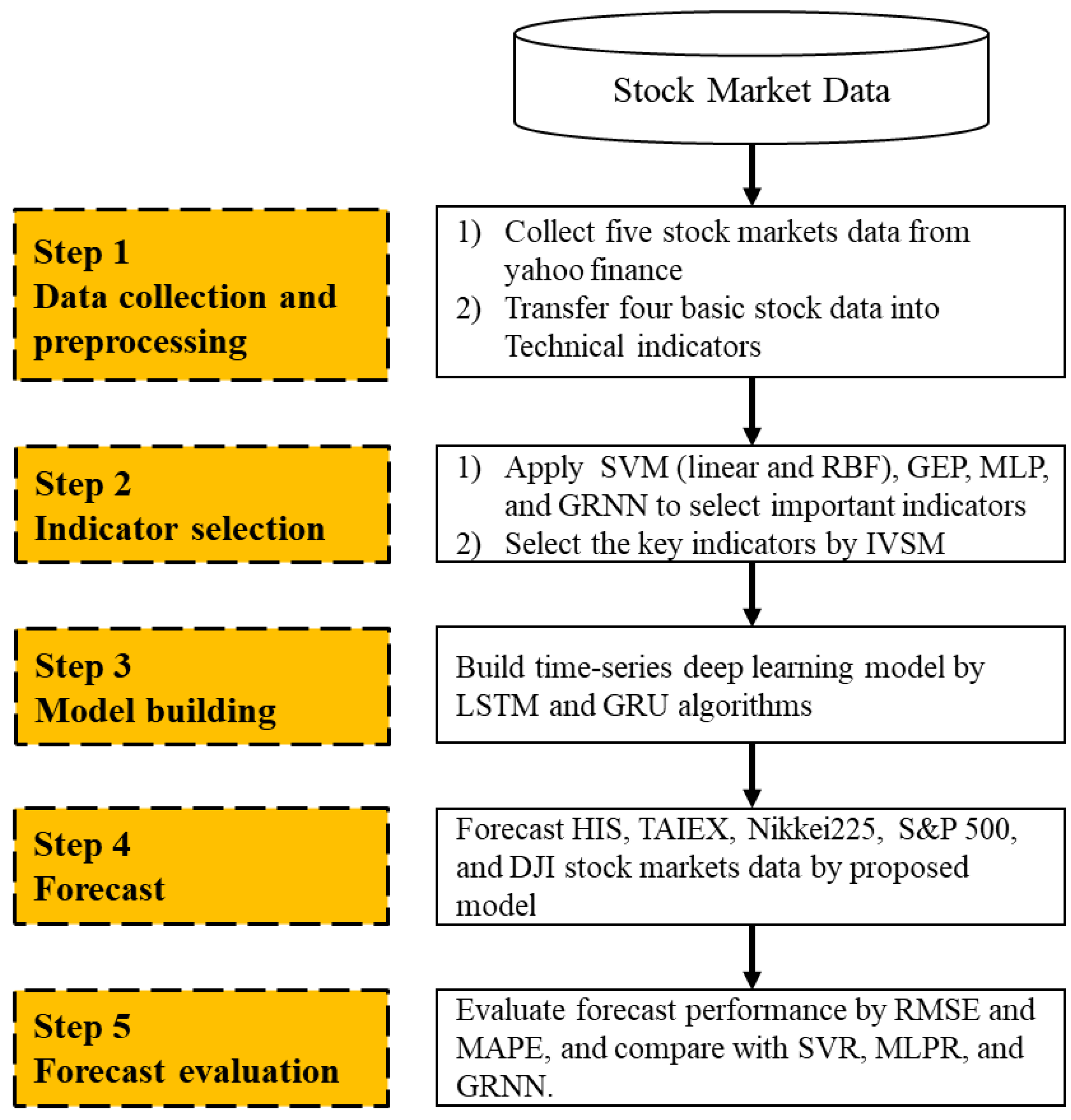
3.1. Proposed Computational Steps
- Step 1: Data collection and preprocessing
- Step 2: Indicator selection
- Step 3: Model building
- Step 4: Forecast
- Step 5: Forecast evaluation
3.2. Proposed Trading Policy
| Algorithm 1: Proposed Trading “Policy 1” |
| Input: forecast_close, actual_close, actual_open, forecast_length Output: profit
|
4. Experiments and Results
4.1. Experimental Environment
4.2. Experiment and Comparison
- (A)
- Key indicators
- (B) Descriptive statistics
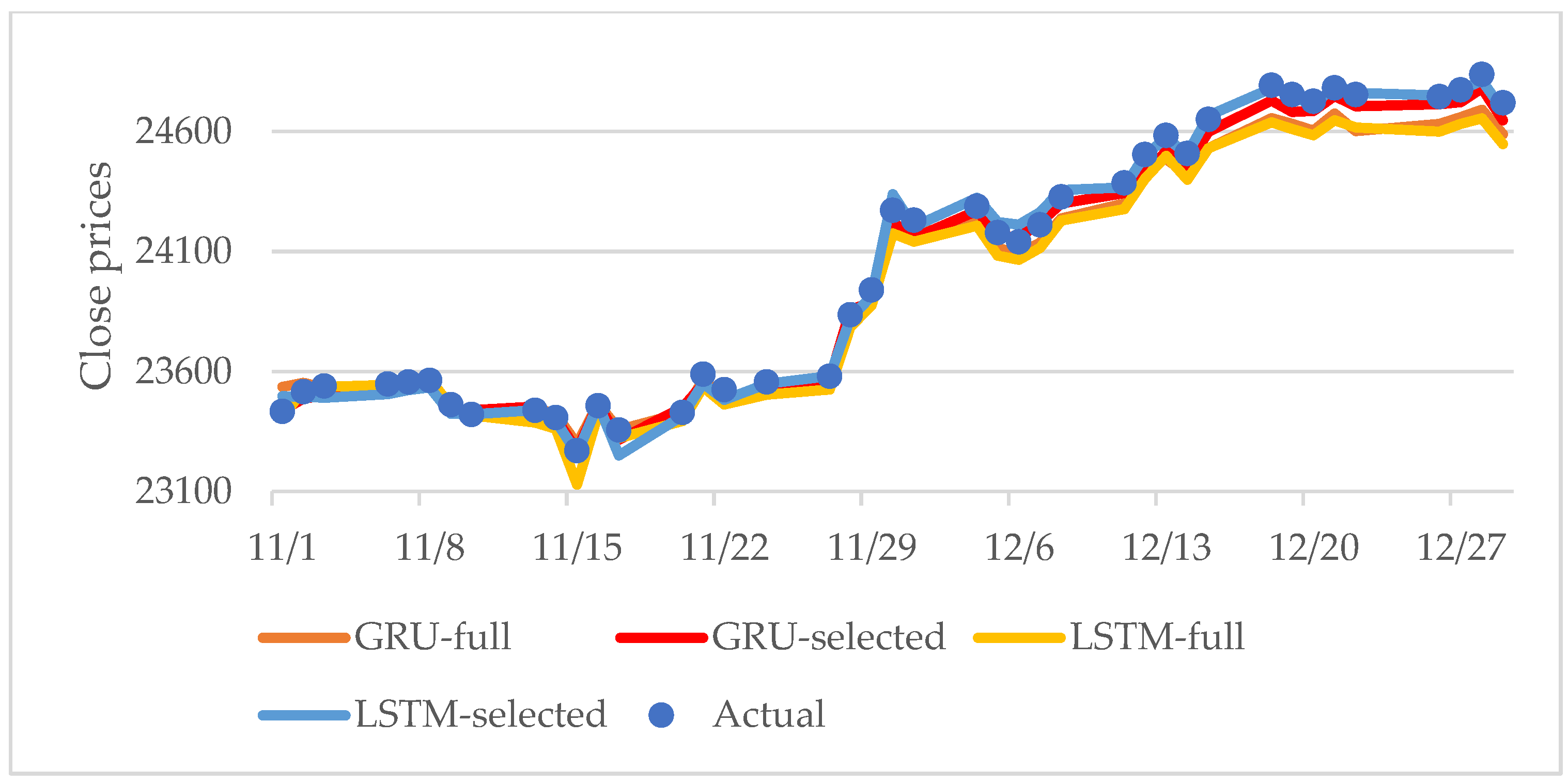
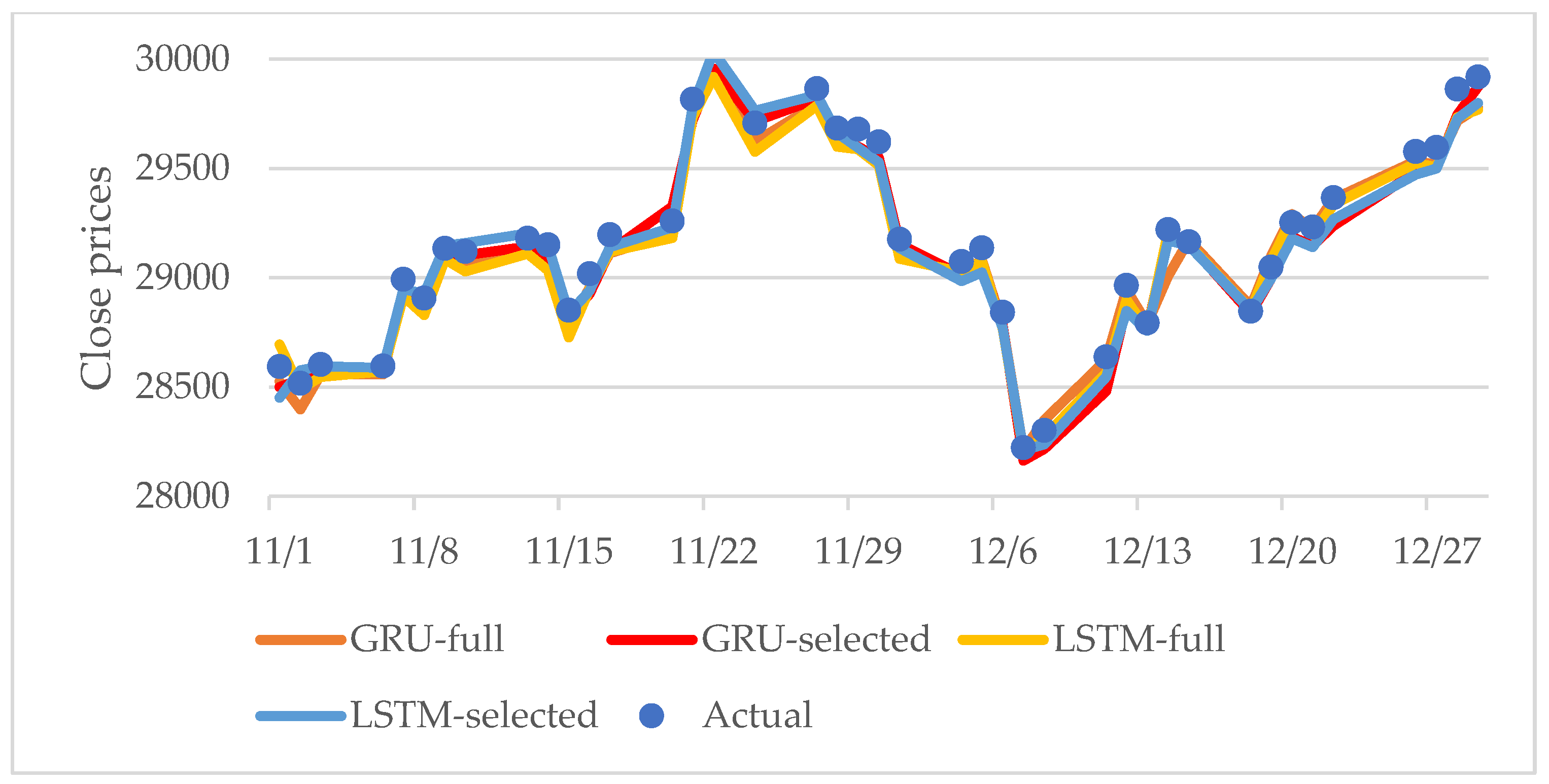
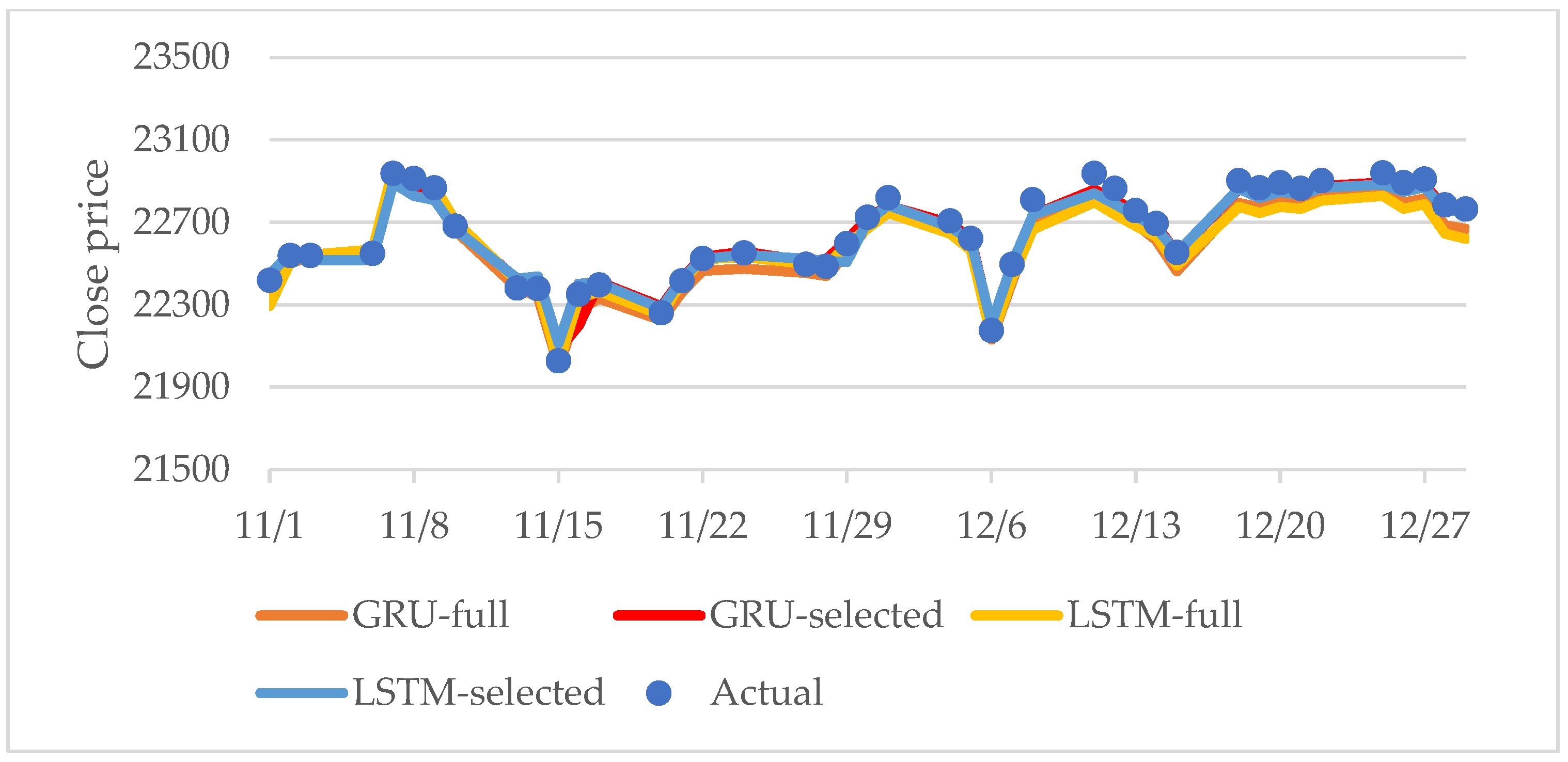
- (C) Forecast comparison
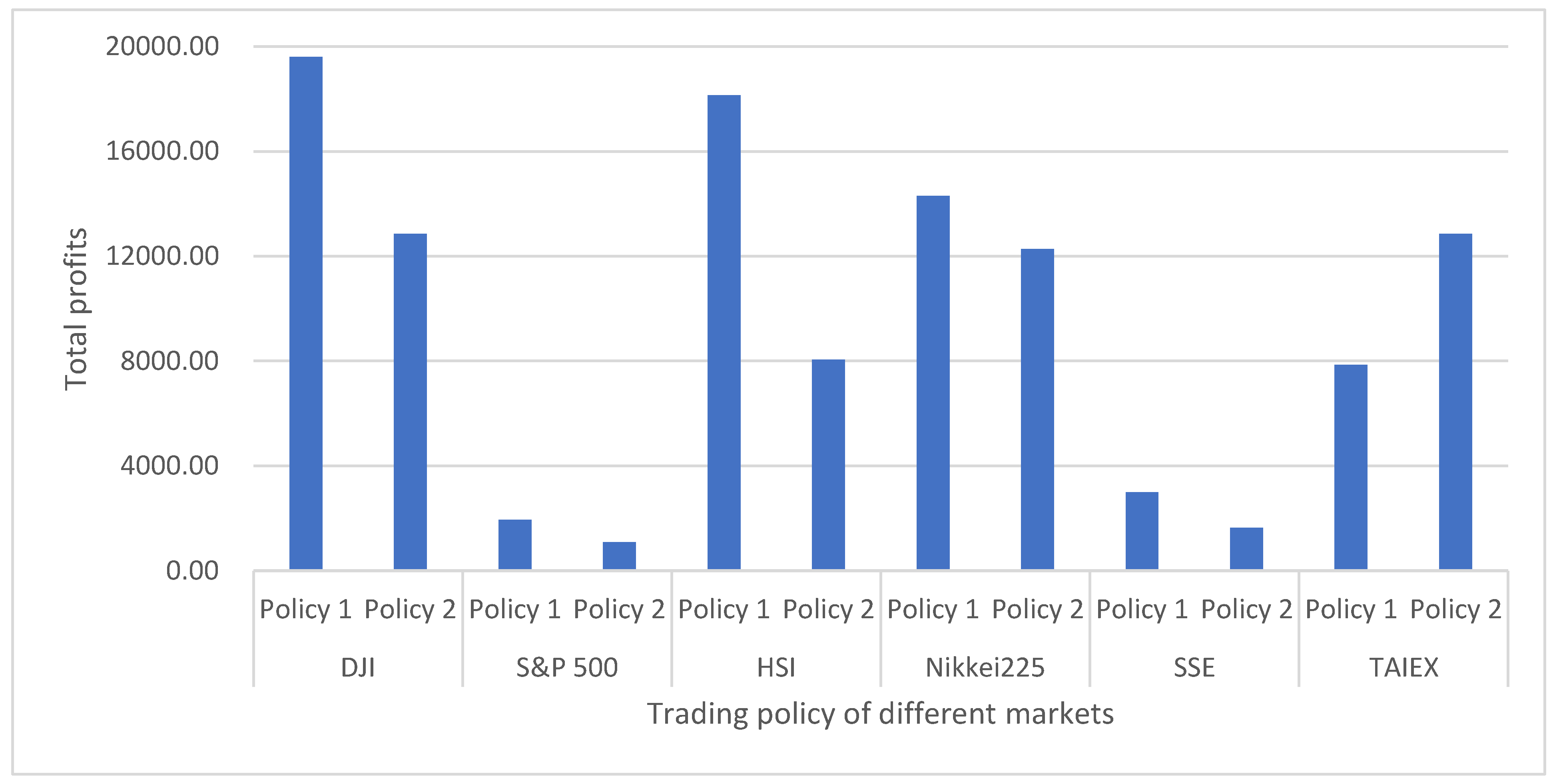
4.3. Profit Comparison
4.4. Discussion and Practical Applicability
- (1)
- Selecting key indicators
- (2)
- Fluctuation and forecast ability
- (3)
- LSTM and GRU advantages
- (4)
- Trading policy
- (5)
- Research hypothesis
- (6)
- Practical applicability
- From the market profits perspective and each year’s investment in six markets, we find the benchmarks as follows.
- (i)
- In terms of profits of six markets, we see that the Dow Jones stock market has the most profits, as shown in Table 11, and then we set the Dow Jones stock market as the benchmark.
- (ii)
- From profits of each year for six markets (as Table 9), we observe that 2019 (HSI, GRU_full), 2018 (DJI, GRU_selected), 2017 (HSI, LSTM_selected), 2016 (Nikkei, GRU_selected), 2015 (DJI, LSTM_selected), 2014 (HSI, LSTM_selected), 2013 (HIS, GRU_selected), 2012 (Nikkei, GRU_full), 2011 (DJI, GRU_selected) can be marked as benchmarks.
- Based on the results of this study, we provide four suggestions for investors as references.
- (i)
- Consider the eight technical indicators (LAG, EMA, MA, BIAS, MO, BB, DIF, and MCAD) and add their own practical experience in analyzing stock price trends.
- (ii)
- Apply GRU combined with the selected key indicators to forecast stock prices because the proposed model can accelerate execution and reduce memory consumption.
- (iii)
- Use one step ahead to forecast stock prices because it can accurately reflect the trading situations of investors in the stock market.
- (iv)
- Employ the proposed trading policy 1 in the six stock markets and could consider the proposed trading policy 2 in the TAIEX stock market.
- (7)
- Opportunity costs
5. Conclusions
- (1)
- This study collects technical indicators that have appeared in recent high-quality journals and financial market transactions, and then we summarize the technical indicators that frequently recur in the collected literature as the technical indicators of this study.
- (2)
- This paper proposes the IISM method to integrate the results of MLPR, SVR, GRNN, and GEP indicator selection and find 15 key technical indicators. These 15 indicators can be summarized as eight technical indicators: LAG, EMA, MA, BIAS, MO, BB, DIF, and MCAD.
- (3)
- This study proposes the combined LSTM and GRU models with the selected key indicators are better than the listing methods in a large fluctuation of stock markets, and we use one-step ahead forecasting to accurately reflect investors’ trading situations in the stock market.
- (4)
- Two trading strategies are proposed, and their profits are compared with the listing methods. The results can provide investors with a reference for future investment.
Author Contributions
Funding
Data Availability Statement
Conflicts of Interest
Abbreviations
| Adam | adaptive moment estimation |
| ANN | artificial neuro network |
| AR | autoregressive |
| ARIMA | autoregressive integrated moving average |
| BB | Bollinger band |
| BIAS | bias lags |
| DEM | Demand index |
| DIF | difference |
| DJI | Dow Jones industrial average |
| DL | deep learning |
| EMA | exponential moving average |
| EMH | efficient market hypothesis |
| GEP | gene expression programming |
| GRNN | generalized regression neural network |
| GRU | gated recurrent units |
| HSI | Hang Seng index |
| I | integral |
| IISM | integrated indicator selection method |
| IVSM | integrated support vector machine |
| K%D | stochastic line |
| LAG | lag period |
| LSTM | long short-term memory |
| MA | moving average |
| MACD | moving average convergence and divergence |
| MAPE | mean absolute percentage error |
| MLP | multilayer perceptron |
| MLPR | multilayer perceptron regression |
| MO | momentum |
| Nikkei 225 | Nikkei average index |
| OSC | Oscillator |
| PROC | price rate of change |
| PSY | psychological line |
| RBF | radial basis function |
| RDP | relative differences in percentage |
| RMSE | root mean square error |
| RNN | recurrent neural network |
| RSI | relative strength index |
| S&P 500 | Standard & Poor’s index |
| SSE | Shanghai Stock Exchange (China A Shares). |
| SVM | support vector machine |
| SVR | support vector regression |
| TAIEX | Taiwan weighted index |
| Volume | basic trading volume |
| WMS%R | William indicator |
Appendix A

| Stock Index | Description |
|---|---|
| HSI | The HSI is an important indicator that reflects the Hong Kong stock market, and the index is calculated from the market value of fifty constituent stocks of the Hang Seng Index. |
| TAIEX | TAIEX is a weighted index of Taiwan, which is regarded as an indicator of the trend of Taiwan’s economy. |
| Nikkei 225 | Nikkei 225 is a stock price index of 225 varieties of the Tokyo Stock Exchange. |
| S&P 500 | The US Standard & Poor 500 is the average record of the US stock market since 1957, covering 500 listed companies in the US. |
| DJI | The Dow Jones industrial average includes the 30 largest and most well-known listed companies in the United States. |
| SSE | The Shanghai Stock Exchange (SSE) is one of the two Chinese A shares. |
| Indicator | Description | Reference |
|---|---|---|
| MA(5) MA(20) | Moving average is used to underline the direction of a trend and smooth out price and volume fluctuations, and it is defined in the following: MA(n) = , where n = 5, and 20. | Kannan et al. [57] |
| BB up BB down | A Bollinger band defined by a set of trend lines plotted two standard deviations (positively and negatively) away from a simple moving average (MA) of a security’s price. | Leung and Chong [20] |
| RDP(1) | The actual closing price is transformed into a relative difference in the percentage of the price, and it is defined in the following formula: RDP(1) = . | Tay and Cao [1] |
| BIAS(6) BIAS(12) BIAS(24) | Bias ratio is the difference between closing price and moving average, and it is defined in the following formula: , where t = 6, 12, and 24. | Chang et al. [21] |
| RSI | The relative strength index shows the most recent stock profit and loss comparison, and the purpose is to determine the overbought and oversold conditions of assets. | Tsai et al. [19] |
| EMA(12) EMA(26) | The exponential moving average is calculated by the weighted average from the current price to the past price, and it is defined as follows: α = . | Nakano et al. [58] |
| MACD (DEM) DIF OSC | Moving average convergence/divergence shows the difference between the fast and slow exponential moving average of the closing price, and MACD is composed of three elements: difference (DIF), Demand index (DEM, signal line also called MACD), Oscillator (OSC). They are defined as follows: DIF , and . | Ahmar [22] |
| PSY(12) PSY(24) | The psychological line is a ratio of rising over a period, and it reflects the purchasing power relative to the sales ability. It is defined as follows: PSY(N) = , where N = 12, and 24. | Lai et al. [23] |
| WMS%R | Williams %R is a momentum indicator range from 0 to −100, and it is used to measure overbought and oversold levels. Williams %R can be used to find market entry and exit points, and this indicator is very similar to the stochastic %K and %D. | Naik and Mohan [59] |
| Stochastic K% Stochastic D% | Stochastic oscillator %K and %D are momentum indicators, which can show the position relative to the high/low range over a period of time. | Chang and Fan [60] |
| PROC | Percentage of price change measures the percentage change in price between the current price and the price of a certain number of periods ago. | Anish and Majhi [61] |
| MO(1) | Momentum measures the amount of change in security prices in a given time and displays the rate of change in stock prices, and its formula is defined as follows: . | Tanaka-Yamawaki et al. [62] |
| LAG(1) | The first-order lag period, and the formula is defined as follows: LAG(1) = Price(t−1). | Chen et al. [12] |
| Volume | Trading volume is a measure of the completed transactions of specific security within a specific period of time. It measures two very important factors: market activity and liquidity. | Ahmar [22] |
References
- Tay, F.E.H.; Cao, L. Application of support vector machines in financial time series forecasting. Omega 2001, 29, 309–317. [Google Scholar] [CrossRef]
- Fama, E.F. Random Walk in Stock Market Prices. Financ. Anal. J. 1995, 51, 75–80. [Google Scholar] [CrossRef] [Green Version]
- Abu-Mostafa, Y.S.; Atiya, A.F. Introduction to financial forecasting. Appl. Intell. 1996, 6, 205–213. [Google Scholar] [CrossRef]
- Ariyo, A.A.; Adewumi, A.O.; Ayo, C.K. Stock price prediction using the ARIMA model. In Proceedings of the 2014 UKSim-AMSS 16th International Conference on Computer Modelling and Simulation, Cambridge, UK, 26–28 March 2014; pp. 106–112. [Google Scholar] [CrossRef] [Green Version]
- Bao, W.; Yue, J.; Rao, Y. A deep learning framework for financial time series using stacked autoencoders and long-short term memory. PLoS ONE 2017, 12, e0180944. [Google Scholar] [CrossRef] [Green Version]
- Barak, S.; Modarres, M. Developing an approach to evaluate stocks by forecasting effective features with data mining methods. Expert Syst. Appl. 2015, 42, 1325–1339. [Google Scholar] [CrossRef]
- Chen, K.; Zhou, Y.; Dai, F. A LSTM-based method for stock returns prediction: A case study of China stock market. In Proceedings of the 2015 IEEE International Conference on Big Data (Big Data), Santa Clara, CA, USA, 29 October–1 November 2015; pp. 2823–2824. [Google Scholar] [CrossRef]
- Chong, E.; Han, C.; Park, F.C. Deep learning networks for stock market analysis and prediction: Methodology, data representations, and case studies. Expert Syst. Appl. 2017, 83, 187–205. [Google Scholar] [CrossRef] [Green Version]
- Fischer, T.; Krauss, C. Deep learning with long short-term memory networks for financial market predictions. Eur. J. Oper. Res. 2018, 270, 654–669. [Google Scholar] [CrossRef] [Green Version]
- Nassirtoussi, A.K.; Aghabozorgi, S.; Wah, T.Y.; Ngo, D.C.L. Text mining of news-headlines for FOREX market prediction: A multilayer dimension reduction algorithm with semantics and sentiment. Expert Syst. Appl. 2015, 42, 306–324. [Google Scholar] [CrossRef]
- Nobre, J.; Neves, R.F. Combining principal component analysis, discrete wavelet transform and XGBoost to trade in the financial markets. Expert Syst. Appl. 2019, 125, 181–194. [Google Scholar] [CrossRef]
- Chen, T.L.; Cheng, C.H.; Liu, J.W. A Causal Time-Series Model Based on Multilayer Perceptron Regression for Forecasting Taiwan Stock Index. Int. J. Inf. Technol. Decis. Mak. 2019, 18, 1967–1987. [Google Scholar] [CrossRef]
- Franses, P.H.; Ghijsels, H. Additive outliers, GARCH and forecasting volatility. Int. J. Forecast. 1999, 15, 1–9. [Google Scholar] [CrossRef]
- Zhang, J.; Xie, Y.; Li, Y.; Shen, C.; Xi, Y. COVID-19 Screening on Chest X-ray Images Using Deep Learning based Anomaly Detection. arXiv 2020, arXiv:2003.12338. [Google Scholar]
- Cowles, A., 3rd. Can Stock Market Forecasters Forecast? Econometrica 1933, 1, 309–324. [Google Scholar] [CrossRef] [Green Version]
- Neely, C.J.; Rapach, D.E.; Tu, J.; Zhou, G. Forecasting the equity risk premium: The role of technical indicators. Manag. Sci. 2014, 60, 1772–1791. [Google Scholar] [CrossRef] [Green Version]
- Peng, Y.; Albuquerque, P.H.M.; Kimura, H.; Saavedra, C.A.P.B. Feature selection and deep neural networks for stock price direction forecasting using technical analysis indicators. Mach. Learn. Appl. 2021, 5, 100060. [Google Scholar] [CrossRef]
- Wang, Y.; Liu, L.; Wu, C. Forecasting commodity prices out-of-sample: Can technical indicators help? Int. J. Forecast. 2020, 36, 666–683. [Google Scholar] [CrossRef]
- Tsai, C.F.; Lin, Y.C.; Yen, D.C.; Chen, Y.M. Predicting stock returns by classifier ensembles. Appl. Soft Comput. 2011, 11, 2452–2459. [Google Scholar] [CrossRef]
- Leung, J.M.J.; Chong, T.T.L. An empirical comparison of moving average envelopes and Bollinger Bands. Appl. Econ. Lett. 2003, 10, 339–341. [Google Scholar] [CrossRef]
- Chang, P.C.; Liao, T.W.; Lin, J.J.; Fan, C.Y. A dynamic threshold decision system for stock trading signal detection. Appl. Soft Comput. 2011, 11, 3998–4010. [Google Scholar] [CrossRef]
- Ahmar, A.S. Sutte Indicator: A Technical Indicator in Stock Market. Int. J. Econ. Financ. Issues 2017, 7, 223–226. Available online: https://dergipark.org.tr/en/pub/ijefi/issue/32035/354468 (accessed on 10 July 2021).
- Lai, H.W.; Chen, C.W.; Huang, C.S. Technical analysis, investment psychology, and liquidity provision: Evidence from the Taiwan stock market. Emerg. Mark. Financ. Trade 2010, 46, 18–38. [Google Scholar] [CrossRef]
- Verleysen, M.; François, D. The curse of dimensionality in data mining and time series prediction. In Computational Intelligence and Bioinspired Systems, Proceedings of the International Work-Conference on Artificial Neural Networks, Warsaw, Poland, 10–15 September 2005; Lecture Notes in Computer, Science; Cabestany, J., Prieto, A., Sandoval, F., Eds.; Springer: Berlin/Heidelberg, Germany, 2005; Volume 3512, pp. 758–770. [Google Scholar] [CrossRef]
- Chandrashekar, G.; Sahin, F. A survey on feature selection methods. Comput. Electr. Eng. 2014, 40, 16–28. [Google Scholar] [CrossRef]
- Guyon, I.; Elisseeff, A. An Introduction of Variable and Feature Selection. J. Mach. Learn. Res. 2003, 3, 1157–1182. [Google Scholar]
- Guyon, I.; Weston, J.; Barnhill, S.; Vapnik, V. Gene selection for cancer classification using support vector machines. Mach. Learn. 2002, 46, 389–422. [Google Scholar] [CrossRef]
- Van Der Malsburg, C.; Rosenblatt, F. Principles of neurodynamics: Perceptrons and the theory of brain mechanisms. In Brain Theory; Palm, G., Aertsen, A., Eds.; Springer: Berlin/Heidelberg, Germany, 1986; pp. 245–248. [Google Scholar] [CrossRef]
- Sezer, O.B.; Gudelek, M.U.; Ozbayoglu, A.M. Financial time series forecasting with deep learning: A systematic literature review: 2005–2019. Appl. Soft Comput. 2020, 90, 106181. [Google Scholar] [CrossRef] [Green Version]
- Lee, S.-J.; Tseng, C.-H.; Lin, G.T.–R.; Yang, Y.; Yang, P.; Muhammad, K.; Pandey, H.M. A dimension-reduction based multilayer perception method for supporting the medical decision making. Pattern Recognit. Lett. 2020, 131, 15–22. [Google Scholar] [CrossRef]
- Cortes, C.; Vapnik, V. Support vector machine. Mach. Learn. 1995, 20, 273–297. [Google Scholar] [CrossRef]
- Yang, H.; Chan, L.; King, I. Support vector machine regression for volatile stock market prediction. In Intelligent Data Engineering and Automated Learning—IDEAL 2002, Proceedings of the International Conference on Intelligent Data Engineering and Automated Learning, Manchester, UK, 24–26 November 2002; Yin, H., Allinson, N., Freeman, R., Keane, J., Hubbard, S., Eds.; Lecture Notes in Computer Science; Springer: Berlin/Heidelberg, Germany, 2002; Volume 2412, p. 2412. [Google Scholar] [CrossRef]
- Karmy, J.P.; Maldonado, S. Hierarchical time series forecasting via support vector regression in the European travel retail industry. Expert Syst. Appl. 2019, 137, 59–73. [Google Scholar] [CrossRef]
- Crone, S.F.; Guajardo, J.; Weber, R. The impact of preprocessing on support vector regression and neural networks in time series prediction. In Proceedings of the International Conference on Data Mining DMIN’06, Las Vegas, NV, USA, 26–29 June 2006; CSREA: Providence, RI, USA; pp. 37–42. [Google Scholar]
- Specht, D.F. A general regression neural network. IEEE Trans. Neural Netw. 1991, 2, 568–576. [Google Scholar] [CrossRef] [Green Version]
- Ferreira, C. Gene Expression Programming: A New Adaptive Algorithm for Solving Problems. arXiv 2001, arXiv:0102027. [Google Scholar] [CrossRef]
- Wang, B.; Li, T.; Yan, Z.; Zhang, G.; Lu, J. Deep PIPE: A distribution-free uncertainty quantification approach for time series forecasting. Neurocomputing 2020, 397, 11–19. [Google Scholar] [CrossRef]
- Box, G.E.P.; Jenkins, G.M. Time Series Analysis: Forecasting and Control; Holden-Day: San Francisco, CA, USA, 1976. [Google Scholar]
- Hyndman, R.J.; Athanasopoulos, G. Forecasting: Principles and Practice, 3rd ed.; OTexts: Melbourne, Australia, 2021. [Google Scholar]
- Hochreiter, S.; Schmidhuber, J. Long short-term memory. Neural Comput. 1997, 9, 1735–1780. [Google Scholar] [CrossRef]
- Kim, T.; Kim, H.Y. Forecasting stock prices with a feature fusion LSTM-CNN model using different representations of the same data. PLoS ONE 2019, 14, e0212320. [Google Scholar] [CrossRef] [Green Version]
- Cho, K.; van Merrienboer, B.; Bahdanau, D.; Bengio, Y. On the properties of neural machine translation: Encoder-decoder approaches. arXiv 2014, arXiv:1409.1259. [Google Scholar] [CrossRef]
- Wang, W.; Yang, N.; Wei, F.; Chang, B.; Zhou, M. R-NET: Machine Reading Comprehension with Self-Matching Networks; Technical Report 5; Natural Language Computer Group, Microsoft Research Asia: Beijing, China, 2017. [Google Scholar]
- Man, J.; Dong, H.; Yang, X.; Meng, Z.; Jia, L.; Qin, Y.; Xin, G. GCG: Graph Convolutional network and gated recurrent unit method for high-speed train axle temperature forecasting. Mech. Syst. Signal Process. 2022, 163, 108102. [Google Scholar] [CrossRef]
- Tan, C.N.W. A hybrid financial trading system incorporating chaos theory, statistical and artificial intelligence/soft computing methods. In Proceedings of the Queensland Finance Conference, Brisbane, Australia, 30 September–1 October 1999; Available online: http://machine-learning.martinsewell.com/ann/Tan99.pdf (accessed on 1 July 2021).
- The PyData Development Team, Python Programming Language. Available online: https://pypi.org/project/pandas-datareader/ (accessed on 1 July 2021).
- Yahoo Finance. Available online: https://finance.yahoo.com/ (accessed on 10 July 2021).
- Financial Transactions Taxes around the World. Available online: https://cepr.net/report/financial-transactions-taxes-around-the-world/ (accessed on 10 November 2022).
- Chen, Y.S.; Cheng, C.H.; Chiu, C.L.; Huang, S.T. A study of ANFIS-based multi-factor time series models for forecasting stock index. Appl. Intell. 2016, 45, 277–292. [Google Scholar] [CrossRef]
- Chang, C.-C.; Lin, C.-J. LIBSVM: A library for support vector machines. ACM Trans. Intell. Syst. Technol. 2011, 2, 1–27. [Google Scholar] [CrossRef]
- Busch, T.; Christensen, B.J.; Nielsen, M.Ø. The role of implied volatility in forecasting future realized volatility and jumps in foreign exchange, stock, and bond markets. J. Econom. 2011, 160, 48–57. [Google Scholar] [CrossRef]
- Ending 10-Year Financial Crisis. 2017. Available online: https://www.marketwatch.com/story/financial-crisis-is-now-officially-over-and-heres-the-chart-that-proves-it-2017-12-01 (accessed on 10 July 2021).
- China’s Stock Market Crash: One Year Later. 2016. Available online: https://www.forbes.com/sites/sarahsu/2016/07/13/chinas-stock-market-crash-one-year-later/?sh=63a9e1335503 (accessed on 10 July 2021).
- LeCun, Y.; Bengio, Y.; Hinton, G. Deep learning. Nature 2015, 521, 436–444. [Google Scholar] [CrossRef]
- Shi, Y.; Li, W.; Zhu, L.; Guo, K.; Cambria, E. Stock trading rule discovery with double deep Q-network. Appl. Soft Comput. 2021, 107, 107320. [Google Scholar] [CrossRef]
- Du, N.; Yan, Y.; Qin, Z. Analysis of financing strategy in coopetition supply chain with opportunity cost. Eur. J. Oper. Res. 2022, 305, 85–100. [Google Scholar] [CrossRef]
- Kannan, K.S.; Sekar, P.S.; Sathik, M.M.; Arumugam, P. Financial stock market forecast using data mining techniques. In Proceedings of the International Multiconference of Engineers and Computer Scientists, Hong Kong, China, 17–19 March 2010. [Google Scholar]
- Nakano, M.; Takahashi, A.; Takahashi, S. Generalized exponential moving average (EMA) model with particle filtering and anomaly detection. Expert Syst. Appl. 2017, 73, 187–200. [Google Scholar] [CrossRef]
- Naik, N.; Mohan, B.R. Optimal feature selection of technical indicator and stock prediction using machine learning technique. In Proceedings of the International Conference on Emerging Technologies in Computer Engineering, Jaipur, India, 1–2 February 2019; Springer: Singapore, 2019; pp. 261–268. [Google Scholar] [CrossRef]
- Chang, P.C.; Fan, C.Y. A hybrid system integrating a wavelet and TSK fuzzy rules for stock price forecasting. IEEE Trans. Syst. Man Cybern. Part C Appl. Rev. 2008, 38, 802–815. [Google Scholar] [CrossRef]
- Anish, C.M.; Majhi, B. Hybrid nonlinear adaptive scheme for stock market prediction using feedback FLANN and factor analysis. J. Korean Stat. Soc. 2016, 45, 64–76. [Google Scholar] [CrossRef]
- Tanaka-Yamawaki, M.; Tokuoka, S. Adaptive use of technical indicators for the prediction of intra-day stock prices. Phys. A Stat. Mech. Appl. 2007, 383, 125–133. [Google Scholar] [CrossRef]


| Indicators | SVM-Linear | SVM-RBF | MLPR | GRNN | GEP | IISM |
|---|---|---|---|---|---|---|
| Volume | ||||||
| MA(5) | ✕ | ✕ | ||||
| MA(20) | ✕ | ✕ | ||||
| BB up | ✕ | ✕ | ||||
| BB down | ✕ | ✕ | ✕ | |||
| RSI | ||||||
| EMA(12) | ✕ | ✕ | ✕ | |||
| EMA(26) | ✕ | ✕ | ||||
| DIF | ✕ | ✕ | ||||
| DEM | ||||||
| OSC | ✕ | ✕ | ||||
| RDP | ✕ | ✕ | ||||
| BIAS(6) | ✕ | ✕ | ||||
| BIAS(12) | ✕ | ✕ | ||||
| BIAS(24) | ✕ | ✕ | ||||
| PSY(12) | ||||||
| PSY(24) | ||||||
| W%R | ||||||
| %K | ||||||
| %D | ||||||
| PROC | ||||||
| MO(1) | ✕ | ✕ | ✕ | ✕ | ||
| LAG(1) | ✕ | ✕ | ✕ | ✕ | ✕ |
| Algorithm | Parameter | Reference |
|---|---|---|
| LSTM | # layers: [1, 5]; #nodes per layer: [30, 70]; batch size = [64, 128]; activation function: relu; learning rate: [0.001, 0.1]; epochs: [50, 80]; optimizer: Adam. | Kim and Kim [41] |
| GRU | # layers: [1, 5]; #nodes per layer: 50; batch size= 100; learning rate: [0.001, 0.1]; epochs = 100; optimizer: Adam. | Wang et al. [43] |
| SVR | kernel function: RBF; epsilon = 0.001; gamma = 1/n (n = #variables); C = 1. | Chang and Lin [50] |
| MLPR | activation function: sigmoid; loss function: square error; learning rate = 0.001; hidden layer sizes = 200. | Lee et al. [30] |
| GRNN | Spread of radial basis functions = 0.25; batch size = 64; epochs = 50. | Specht [35] |
| Indicator | DJI | S&P 500 | HSI | Nikkei 225 | SSE | TAIEX | Total |
|---|---|---|---|---|---|---|---|
| LAG | 9 | 9 | 9 | 9 | 9 | 9 | 54 |
| EMA(26) | 9 | 9 | 9 | 8 | 9 | 9 | 53 |
| EMA(12) | 8 | 9 | 9 | 8 | 9 | 9 | 52 |
| MA(5) | 8 | 8 | 7 | 8 | 9 | 7 | 47 |
| BIAS(24) | 7 | 8 | 8 | 7 | 9 | 5 | 44 |
| MO | 6 | 8 | 6 | 7 | 9 | 6 | 42 |
| MA(20) | 7 | 7 | 6 | 6 | 9 | 6 | 41 |
| BB up | 8 | 7 | 7 | 3 | 9 | 5 | 39 |
| BIAS(6) | 7 | 7 | 6 | 5 | 9 | 5 | 39 |
| BB down | 7 | 6 | 6 | 3 | 9 | 6 | 37 |
| DIF | 5 | 6 | 6 | 5 | 9 | 3 | 34 |
| BIAS(12) | 8 | 5 | 4 | 4 | 9 | 2 | 32 |
| DEM | 5 | 4 | 3 | 5 | 9 | 4 | 30 |
| OSC | 6 | 2 | 5 | 1 | 9 | 4 | 27 |
| RDP | 4 | 3 | 2 | 2 | 9 | 2 | 22 |
| %D | 1 | 0 | 0 | 1 | 9 | 0 | 11 |
| PSY(24) | 0 | 1 | 0 | 0 | 9 | 0 | 10 |
| W%R | 0 | 0 | 0 | 1 | 9 | 0 | 10 |
| PROC | 1 | 0 | 0 | 0 | 9 | 0 | 10 |
| PSY(12) | 0 | 0 | 0 | 0 | 9 | 0 | 9 |
| RSI | 0 | 0 | 0 | 0 | 9 | 0 | 9 |
| Volume | 0 | 0 | 0 | 0 | 9 | 0 | 9 |
| %K | 0 | 0 | 0 | 0 | 9 | 0 | 9 |
| Stock | Year | Range | Standard Deviation | Max | Min |
|---|---|---|---|---|---|
| DJI | 2019 | 5959.04 | 1073.00 | 28,645.26 | 22,686.22 |
| 2018 | 5036.19 | 829.17 | 26,828.39 | 21,792.20 | |
| 2017 | 5105.11 | 1322.01 | 24,837.51 | 19,732.40 | |
| 2016 | 4314.44 | 942.76 | 19,974.62 | 15,660.18 | |
| 2015 | 2645.95 | 554.69 | 18,312.39 | 15,666.44 | |
| 2014 | 2680.91 | 552.71 | 18,053.71 | 15,372.80 | |
| 2013 | 3247.81 | 715.71 | 16,576.66 | 13,328.85 | |
| 2012 | 1508.69 | 319.39 | 13,610.15 | 12,101.46 | |
| 2011 | 2155.24 | 490.41 | 12,810.54 | 10,655.30 | |
| S&P 500 | 2019 | 792.13 | 150.67 | 3240.02 | 2447.89 |
| 2018 | 579.65 | 100.41 | 2930.75 | 2351.10 | |
| 2017 | 432.33 | 109.42 | 2690.16 | 2257.83 | |
| 2016 | 442.64 | 101.43 | 2271.72 | 1829.08 | |
| 2015 | 263.21 | 54.89 | 2130.82 | 1867.61 | |
| 2014 | 348.68 | 79.57 | 2090.57 | 1741.89 | |
| 2013 | 391.21 | 99.24 | 1848.36 | 1457.15 | |
| 2012 | 188.71 | 46.63 | 1465.77 | 1277.06 | |
| 2011 | 264.38 | 62.55 | 1363.61 | 1099.23 | |
| HSI | 2019 | 5093.13 | 1247.35 | 30,157.49 | 25,064.36 |
| 2018 | 8568.59 | 2208.93 | 33,154.12 | 24,585.53 | |
| 2017 | 7869.02 | 2134.01 | 30,003.49 | 22,134.47 | |
| 2016 | 5780.12 | 1457.07 | 24,099.70 | 18,319.58 | |
| 2015 | 7886.15 | 2119.41 | 28,442.75 | 20,556.60 | |
| 2014 | 4135.79 | 912.62 | 25,317.95 | 21,182.16 | |
| 2013 | 4224.57 | 877.13 | 24,038.55 | 19,813.98 | |
| 2012 | 4481.00 | 1085.94 | 22,666.59 | 18,185.59 | |
| 2011 | 8169.35 | 2196.81 | 24,419.62 | 16,250.27 | |
| Nikkei 225 | 2019 | 4504.16 | 992.54 | 24,066.12 | 19,561.96 |
| 2018 | 5114.88 | 855.80 | 24,270.62 | 19,155.74 | |
| 2017 | 4603.55 | 1278.82 | 22,939.18 | 18,335.63 | |
| 2016 | 4542.51 | 918.94 | 19,494.53 | 14,952.02 | |
| 2015 | 4072.07 | 1073.36 | 20,868.03 | 16,795.96 | |
| 2014 | 4025.48 | 998.47 | 17,935.64 | 13,910.16 | |
| 2013 | 5804.32 | 1436.01 | 16,291.31 | 10,486.99 | |
| 2012 | 2099.55 | 487.39 | 10,395.18 | 8295.63 | |
| 2011 | 2697.52 | 738.56 | 10,857.53 | 8160.01 | |
| SSE | 2019 | 932.18 | 242.61 | 3201.55 | 2269.37 |
| 2018 | 525.64 | 143.53 | 2577.60 | 2051.96 | |
| 2017 | 507.63 | 116.28 | 2548.30 | 2040.67 | |
| 2016 | 1305.66 | 303.04 | 3389.40 | 2083.74 | |
| 2015 | 2344.22 | 559.22 | 5410.86 | 3066.64 | |
| 2014 | 739.56 | 140.37 | 3518.54 | 2778.98 | |
| 2013 | 414.04 | 102.66 | 3610.86 | 3196.82 | |
| 2012 | 1128.30 | 310.97 | 3728.35 | 2600.05 | |
| 2011 | 845.47 | 165.05 | 3425.90 | 2580.43 | |
| TAIEX | 2019 | 2739.94 | 569.97 | 12,122.45 | 9382.51 |
| 2018 | 1774.12 | 490.46 | 11,253.11 | 9478.99 | |
| 2017 | 1581.69 | 422.65 | 10,854.57 | 9272.88 | |
| 2016 | 1728.67 | 445.92 | 9392.68 | 7664.01 | |
| 2015 | 2562.78 | 605.50 | 9973.12 | 7410.34 | |
| 2014 | 1304.69 | 302.98 | 9569.17 | 8264.48 | |
| 2013 | 1006.79 | 227.44 | 8623.43 | 7616.64 | |
| 2012 | 1249.38 | 296.45 | 8144.04 | 6894.66 | |
| 2011 | 2512.02 | 765.29 | 9145.35 | 6633.33 |
| Stock | Year | LSTM | GRU | MLPR | SVR | GRNN |
|---|---|---|---|---|---|---|
| DJI | 2019 | 97.3619 | 51.7777 | 99.1505 | 226.4525 | 124.4413 |
| 2018 | 42.0281 | 22.5761 | 85.8237 | 353.1809 | 71.8418 | |
| 2017 | 173.9153 | 143.5100 | 657.7406 | 157.9160 | 388.5301 | |
| 2016 | 101.4298 | 74.8453 | 443.3431 | 194.2021 | 155.9858 | |
| 2015 | 91.3310 | 65.6631 | 169.0027 | 175.3816 | 155.0431 | |
| 2014 | 135.6274 | 72.8003 | 693.7565 | 86.8626 | 243.2861 | |
| 2013 | 213.4277 | 111.6285 | 884.4591 | 171.4828 | 370.3082 | |
| 2012 | 157.5769 | 107.6936 | 589.0921 | 72.2888 | 324.3755 | |
| 2011 | 163.9555 | 145.9973 | 847.9486 | 108.9804 | 463.2501 | |
| SD | 52.3746 | 41.6598 | 313.0758 | 84.8945 | 136.8538 | |
| S&P 500 | 2019 | 10.8071 | 6.9224 | 14.8007 | 31.3726 | 13.4845 |
| 2018 | 9.7608 | 8.4751 | 16.3937 | 37.4393 | 11.1921 | |
| 2017 | 20.7944 | 17.0222 | 75.1404 | 16.3912 | 32.1713 | |
| 2016 | 12.8238 | 11.8668 | 48.6820 | 21.0041 | 23.8996 | |
| 2015 | 8.5625 | 4.7605 | 16.9509 | 13.3877 | 12.9853 | |
| 2014 | 15.0190 | 9.2067 | 49.3075 | 9.8192 | 30.7069 | |
| 2013 | 18.6915 | 15.7309 | 70.7076 | 11.9496 | 24.8363 | |
| 2012 | 18.2398 | 12.5796 | 81.8002 | 11.6478 | 39.9090 | |
| 2011 | 18.1740 | 22.4596 | 98.1309 | 18.8881 | 66.5393 | |
| SD | 4.4508 | 5.5588 | 31.2213 | 9.5091 | 17.3052 | |
| HSI | 2019 | 316.9949 | 217.2492 | 557.9458 | 477.9190 | 212.4031 |
| 2018 | 185.3658 | 95.9802 | 767.6190 | 433.5593 | 340.4732 | |
| 2017 | 141.1722 | 95.2021 | 300.0138 | 129.3764 | 208.6685 | |
| 2016 | 95.1898 | 43.1952 | 223.9472 | 535.1239 | 213.4665 | |
| 2015 | 184.5437 | 188.1598 | 481.0047 | 604.0904 | 313.1186 | |
| 2014 | 109.6587 | 91.7758 | 433.2478 | 307.7025 | 274.8683 | |
| 2013 | 224.3597 | 168.7230 | 1016.1220 | 306.6685 | 637.5018 | |
| 2012 | 233.5597 | 191.6585 | 732.3858 | 508.6721 | 372.1900 | |
| 2011 | 144.0242 | 73.4858 | 203.8428 | 533.7443 | 234.6301 | |
| SD | 69.4365 | 62.1009 | 273.6097 | 150.4325 | 136.0408 | |
| Nikkei 225 | 2019 | 57.9599 | 49.4894 | 295.3367 | 298.1137 | 127.5387 |
| 2018 | 83.2773 | 53.3905 | 153.3542 | 378.5275 | 130.4394 | |
| 2017 | 280.9825 | 144.6442 | 774.5934 | 242.1133 | 578.4405 | |
| 2016 | 211.8529 | 164.1940 | 848.6051 | 294.3882 | 221.5481 | |
| 2015 | 111.8379 | 80.5574 | 211.7121 | 153.1162 | 208.9622 | |
| 2014 | 133.0059 | 89.6691 | 617.4355 | 337.1630 | 348.4478 | |
| 2013 | 200.3073 | 127.0322 | 856.7085 | 281.9635 | 216.8408 | |
| 2012 | 236.8379 | 113.0469 | 531.5152 | 174.4274 | 299.8980 | |
| 2011 | 162.6647 | 79.9200 | 570.1168 | 150.0313 | 245.8809 | |
| SD | 74.1970 | 39.7276 | 268.0202 | 82.2947 | 137.4483 | |
| SSE | 2019 | 29.7301 | 29.8800 | 102.2900 | 46.4902 | 49.1010 |
| 2018 | 16.6400 | 9.5300 | 56.5405 | 33.2105 | 36.1930 | |
| 2017 | 12.8203 | 7.2902 | 14.4606 | 19.4130 | 25.1405 | |
| 2016 | 80.2800 | 74.4705 | 261.64004 | 95.9004 | 124.8202 | |
| 2015 | 55.0205 | 50.8807 | 122.0101 | 60.94002 | 127.8201 | |
| 2014 | 125.4506 | 135.0509 | 71.02005 | 132.1605 | 63.0908 | |
| 2013 | 15.4007 | 8.2401 | 45.8104 | 9.2109 | 18.4502 | |
| 2012 | 24.7209 | 16.3103 | 164.9102 | 28.1808 | 55.5603 | |
| 2011 | 21.0502 | 10.0505 | 22.9203 | 15.2001 | 23.6804 | |
| SD | 38.2229 | 43.1155 | 78.7323 | 41.1520 | 41.4547 | |
| TAIEX | 2019 | 88.0367 | 69.5280 | 291.3393 | 179.6965 | 126.4247 |
| 2018 | 24.2061 | 20.9176 | 79.3684 | 140.0722 | 37.6275 | |
| 2017 | 34.6116 | 15.3331 | 94.6621 | 52.0253 | 56.1027 | |
| 2016 | 36.7029 | 20.0098 | 48.8579 | 84.0364 | 52.4923 | |
| 2015 | 53.9813 | 62.6681 | 97.3140 | 233.4626 | 79.0019 | |
| 2014 | 50.4800 | 32.5281 | 133.7349 | 72.2410 | 62.0565 | |
| 2013 | 48.2094 | 28.3626 | 210.3101 | 61.7355 | 107.9973 | |
| 2012 | 80.5682 | 62.4979 | 217.3168 | 62.0967 | 73.5255 | |
| 2011 | 88.6460 | 52.7298 | 351.2767 | 163.2088 | 207.7405 | |
| SD | 24.0609 | 21.2576 | 104.0482 | 64.7495 | 52.4165 |
| Stock | Year | LSTM | GRU | ANN | SVR | GRNN |
|---|---|---|---|---|---|---|
| DJI | 2019 | 0.1051 | 0.1158 | 0.6568 | 0.7015 | 0.7491 |
| 2018 | 0.1953 | 0.1572 | 0.4546 | 0.7782 | 0.4487 | |
| 2017 | 0.3311 | 0.2634 | 3.6491 | 0.6251 | 2.3657 | |
| 2016 | 0.2907 | 0.2432 | 2.1435 | 0.8352 | 0.6351 | |
| 2015 | 0.0905 | 0.0771 | 0.8452 | 0.8191 | 0.7899 | |
| 2014 | 0.1822 | 0.2006 | 3.3667 | 0.4347 | 1.1278 | |
| 2013 | 0.6415 | 0.7449 | 3.1898 | 0.8959 | 1.2641 | |
| 2012 | 0.0910 | 0.0665 | 1.6236 | 0.4177 | 0.9468 | |
| 2011 | 0.1101 | 0.1060 | 2.6720 | 0.7453 | 1.6184 | |
| SD | 0.1787 | 0.2092 | 1.2300 | 0.1712 | 0.5896 | |
| S&P 500 | 2019 | 0.1511 | 0.2004 | 0.9556 | 0.9748 | 0.8918 |
| 2018 | 0.1682 | 0.1678 | 0.7579 | 1.0429 | 0.6841 | |
| 2017 | 0.3972 | 0.3504 | 3.8025 | 0.5921 | 1.6733 | |
| 2016 | 0.1344 | 0.1441 | 2.0330 | 0.6904 | 0.9894 | |
| 2015 | 0.0510 | 0.0599 | 0.6382 | 0.4788 | 0.5160 | |
| 2014 | 0.2001 | 0.1994 | 1.9914 | 0.4613 | 1.2606 | |
| 2013 | 0.7209 | 0.6858 | 2.4623 | 0.6467 | 0.8736 | |
| 2012 | 0.4888 | 0.5340 | 2.3192 | 0.6147 | 1.0757 | |
| 2011 | 0.1129 | 0.0901 | 2.8558 | 1.1333 | 2.0764 | |
| SD | 0.2202 | 0.2126 | 1.0478 | 0.2490 | 0.4908 | |
| HSI | 2019 | 0.1384 | 0.1036 | 2.1647 | 1.2084 | 0.9528 |
| 2018 | 0.2050 | 0.2921 | 2.9759 | 1.2321 | 1.4674 | |
| 2017 | 0.2332 | 0.2135 | 0.9965 | 0.4194 | 0.7106 | |
| 2016 | 0.1815 | 0.2036 | 0.7085 | 1.9868 | 0.7770 | |
| 2015 | 0.2332 | 0.1306 | 1.2792 | 1.8978 | 1.2360 | |
| 2014 | 0.0763 | 0.0947 | 1.4285 | 0.9783 | 1.0791 | |
| 213 | 0.0969 | 0.0858 | 2.8139 | 0.9257 | 2.0501 | |
| 2012 | 0.1771 | 0.2735 | 1.8250 | 1.6783 | 0.9846 | |
| 2011 | 0.5332 | 0.3242 | 0.6181 | 2.0762 | 0.6318 | |
| SD | 0.1338 | 0.0916 | 0.8641 | 0.5648 | 0.4425 | |
| Nikkei 225 | 2019 | 0.1613 | 0.1411 | 2.5424 | 1.0870 | 1.3619 |
| 2018 | 0.2111 | 0.1214 | 1.1613 | 1.1312 | 1.1193 | |
| 2017 | 0.2701 | 0.2704 | 4.8013 | 0.8888 | 3.5028 | |
| 2016 | 0.4086 | 0.2662 | 3.8207 | 1.2244 | 0.9434 | |
| 2015 | 0.1041 | 0.1206 | 0.8710 | 0.6558 | 0.7938 | |
| 2014 | 0.5697 | 0.3586 | 3.1157 | 1.7105 | 1.6490 | |
| 2013 | 0.9969 | 0.9339 | 2.4652 | 1.7248 | 0.6712 | |
| 2012 | 0.3959 | 0.4214 | 1.5005 | 1.2973 | 0.9242 | |
| 2011 | 0.2169 | 0.1640 | 1.7010 | 1.2880 | 0.7987 | |
| SD | 0.2757 | 0.2571 | 1.2979 | 0.3463 | 0.8790 | |
| SSE | 2019 | 0.9508 | 0.7708 | 3.6202 | 0.9202 | 1.6802 |
| 2018 | 0.6302 | 0.3205 | 2.2905 | 0.3503 | 1.3810 | |
| 2017 | 0.4700 | 0.2206 | 0.4306 | 0.2705 | 0.9405 | |
| 2016 | 2.3406 | 2.1907 | 8.5308 | 2.8108 | 4.1704 | |
| 2015 | 1.2205 | 0.8401 | 2.3502 | 0.8409 | 3.2108 | |
| 2014 | 3.7007 | 3.9608 | 1.8803 | 3.9505 | 1.7520 | |
| 2013 | 0.3802 | 0.1905 | 1.0205 | 0.2701 | 0.4610 | |
| 2012 | 0.7106 | 0.3704 | 4.8008 | 0.4504 | 1.8406 | |
| 2011 | 0.5804 | 0.2203 | 0.5904 | 0.2702 | 0.6407 | |
| SD | 1.1047 | 1.2742 | 2.5611 | 1.3321 | 1.2082 | |
| TAIEX | 2019 | 0.1695 | 0.1864 | 3.2778 | 1.4569 | 1.5666 |
| 2018 | 0.8192 | 0.3551 | 0.7126 | 1.0899 | 0.4074 | |
| 2017 | 0.1392 | 0.1012 | 0.8084 | 0.4337 | 0.5350 | |
| 2016 | 0.1375 | 0.0834 | 0.4093 | 0.8133 | 0.4694 | |
| 2015 | 0.1101 | 0.0985 | 0.7987 | 1.9712 | 0.7389 | |
| 2014 | 0.1093 | 0.0988 | 1.0634 | 0.5856 | 0.5825 | |
| 2013 | 0.0894 | 0.0824 | 1.3757 | 0.6958 | 0.7831 | |
| 2012 | 0.0671 | 0.0549 | 1.3385 | 0.6743 | 0.5374 | |
| 2011 | 0.3384 | 0.5618 | 2.3551 | 1.6077 | 1.5320 | |
| SD | 0.2381 | 0.1697 | 0.9150 | 0.5295 | 0.4440 |
| Stock | Year | LSTM-Full | GRU-Full | LSTM-Selected | GRU-Selected |
|---|---|---|---|---|---|
| DJI | 2019 | 97.3619 | 51.7777 | 39.4330 | 18.0759 |
| 2018 | 42.0281 | 22.5761 | 62.7818 | 40.2506 | |
| 2017 | 173.9153 | 143.5100 | 34.4491 | 41.3938 | |
| 2016 | 101.4298 | 74.8453 | 42.9884 | 30.4705 | |
| 2015 | 91.3310 | 65.6631 | 36.3502 | 13.1950 | |
| 2014 | 135.6274 | 72.8003 | 35.2509 | 32.6963 | |
| 2013 | 213.4277 | 111.6285 | 100.2916 | 115.1564 | |
| 2012 | 157.5769 | 107.6936 | 14.6597 | 10.8675 | |
| 2011 | 163.9555 | 145.9973 | 23.7257 | 27.5259 | |
| S&P 500 | 2019 | 10.8071 | 6.9224 | 5.0976 | 5.5951 |
| 2018 | 9.7608 | 8.4751 | 7.9615 | 9.7416 | |
| 2017 | 20.7944 | 17.0222 | 6.0058 | 6.0531 | |
| 2016 | 12.8238 | 11.8668 | 3.3366 | 3.5705 | |
| 2015 | 8.5625 | 4.7605 | 1.8520 | 2.2277 | |
| 2014 | 15.0190 | 9.2067 | 4.4741 | 3.2928 | |
| 2013 | 18.6915 | 15.7309 | 14.6395 | 13.6991 | |
| 2012 | 18.2398 | 12.5796 | 7.0778 | 6.4937 | |
| 2011 | 18.1740 | 22.4596 | 3.8991 | 4.1650 | |
| HSI | 2019 | 316.9949 | 217.2492 | 21.1144 | 48.3584 |
| 2018 | 185.3658 | 95.9802 | 70.2325 | 84.2238 | |
| 2017 | 141.1722 | 95.2021 | 70.5882 | 69.1719 | |
| 2016 | 95.1898 | 43.1952 | 28.9528 | 32.5897 | |
| 2015 | 184.5437 | 188.1598 | 89.5827 | 114.8543 | |
| 2014 | 109.6587 | 91.7758 | 16.8223 | 19.8055 | |
| 2013 | 224.3597 | 168.7230 | 26.0976 | 24.1908 | |
| 2012 | 233.5597 | 191.6585 | 41.6625 | 53.0337 | |
| 2011 | 144.0242 | 73.4858 | 129.4525 | 77.7150 | |
| Nikkei 225 | 2019 | 57.9599 | 49.4894 | 39.6594 | 33.4971 |
| 2018 | 83.2773 | 53.3905 | 71.2000 | 41.0710 | |
| 2017 | 280.9825 | 144.6442 | 44.6268 | 38.6920 | |
| 2016 | 211.8529 | 164.1940 | 34.4573 | 27.7233 | |
| 2015 | 111.8379 | 80.5574 | 28.2564 | 34.6977 | |
| 2014 | 133.0059 | 89.6691 | 90.9622 | 35.0952 | |
| 2013 | 200.3073 | 127.0322 | 122.6082 | 119.8622 | |
| 2012 | 236.8379 | 113.0469 | 45.8351 | 45.5138 | |
| 2011 | 162.6647 | 79.9200 | 32.0047 | 19.7709 | |
| TAIEX | 2019 | 88.0367 | 69.5280 | 14.3573 | 10.5428 |
| 2018 | 24.2061 | 20.9176 | 60.1481 | 39.2575 | |
| 2017 | 34.6116 | 15.3331 | 13.7590 | 10.3119 | |
| 2016 | 36.7029 | 20.0098 | 14.0579 | 13.1937 | |
| 2015 | 53.9813 | 62.6681 | 17.3921 | 18.3855 | |
| 2014 | 50.4800 | 32.5281 | 12.4865 | 10.9234 | |
| 2013 | 48.2094 | 28.3626 | 7.9346 | 6.3685 | |
| 2012 | 80.5682 | 62.4979 | 5.1908 | 5.5051 | |
| 2011 | 88.6460 | 52.7298 | 23.5639 | 16.0520 |
| Stock | Year | LSTM-Full | GRU-Full | LSTM-Selected | GRU-Selected |
|---|---|---|---|---|---|
| DJI | 2019 | 0.1051 | 0.1158 | 0.1033 | 0.0501 |
| 2018 | 0.1953 | 0.1572 | 0.1560 | 0.1067 | |
| 2017 | 0.3311 | 0.2634 | 0.1079 | 0.1454 | |
| 2016 | 0.2907 | 0.2432 | 0.1787 | 0.1240 | |
| 2015 | 0.0905 | 0.0771 | 0.1358 | 0.0557 | |
| 2014 | 0.1822 | 0.2006 | 0.1683 | 0.1583 | |
| 2013 | 0.6415 | 0.7449 | 0.6043 | 0.7138 | |
| 2012 | 0.0910 | 0.0665 | 0.0799 | 0.0683 | |
| 2011 | 0.1101 | 0.1060 | 0.0857 | 0.0893 | |
| S&P 500 | 2019 | 0.1511 | 0.2004 | 0.1335 | 0.1400 |
| 2018 | 0.1682 | 0.1678 | 0.2243 | 0.2201 | |
| 2017 | 0.3972 | 0.3504 | 0.2133 | 0.2233 | |
| 2016 | 0.1344 | 0.1441 | 0.1216 | 0.1262 | |
| 2015 | 0.0510 | 0.0599 | 0.0554 | 0.0515 | |
| 2014 | 0.2001 | 0.1994 | 0.1788 | 0.1373 | |
| 2013 | 0.7209 | 0.6858 | 0.7956 | 0.7517 | |
| 2012 | 0.4888 | 0.5340 | 0.4268 | 0.3999 | |
| 2011 | 0.1129 | 0.0901 | 0.1578 | 0.1435 | |
| HSI | 2019 | 0.1384 | 0.1036 | 0.0638 | 0.1076 |
| 2018 | 0.2050 | 0.2921 | 0.1826 | 0.2240 | |
| 2017 | 0.2332 | 0.2135 | 0.2009 | 0.2047 | |
| 2016 | 0.1815 | 0.2036 | 0.1012 | 0.1083 | |
| 2015 | 0.2332 | 0.1306 | 0.2846 | 0.3230 | |
| 2014 | 0.0763 | 0.0947 | 0.0546 | 0.0656 | |
| 2013 | 0.0969 | 0.0858 | 0.0776 | 0.0692 | |
| 2012 | 0.1771 | 0.2735 | 0.1153 | 0.1311 | |
| 2011 | 0.5332 | 0.3242 | 0.6327 | 0.3682 | |
| Nikkei 225 | 2019 | 0.1613 | 0.1411 | 0.1363 | 0.1093 |
| 2018 | 0.2111 | 0.1214 | 0.2125 | 0.1433 | |
| 2017 | 0.2701 | 0.2704 | 0.1624 | 0.1229 | |
| 2016 | 0.4086 | 0.2662 | 0.1496 | 0.1180 | |
| 2015 | 0.1041 | 0.1206 | 0.0968 | 0.0837 | |
| 2014 | 0.5697 | 0.3586 | 0.4120 | 0.1755 | |
| 2013 | 0.9969 | 0.9339 | 0.7753 | 0.7625 | |
| 2012 | 0.3959 | 0.4214 | 0.4155 | 0.4266 | |
| 2011 | 0.2169 | 0.1640 | 0.2083 | 0.1130 | |
| TAIEX | 2019 | 0.1695 | 0.1864 | 0.1036 | 0.0716 |
| 2018 | 0.8192 | 0.3551 | 0.5626 | 0.3792 | |
| 2017 | 0.1392 | 0.1012 | 0.1063 | 0.0853 | |
| 2016 | 0.1375 | 0.0834 | 0.1223 | 0.1160 | |
| 2015 | 0.1101 | 0.0985 | 0.1431 | 0.1707 | |
| 2014 | 0.1093 | 0.0988 | 0.0961 | 0.0796 | |
| 2013 | 0.0894 | 0.0824 | 0.0707 | 0.0503 | |
| 2012 | 0.0671 | 0.0549 | 0.0489 | 0.0454 | |
| 2011 | 0.3384 | 0.5618 | 0.2544 | 0.1642 |
| Proposed Policy 1 | Chen et al. [49] | ||||||||
|---|---|---|---|---|---|---|---|---|---|
| Stock | Year | LSTM-Full | GRU- Full | LSTM-Selected | GRU- Selected | LSTM- Full | GRU- Full | LSTM-Selected | GRU-Selected |
| DJI | 2019 | 1828.63 | 1911.68 | 2001.95 | 2081.5 | 235 | 80.85 | −74.39 | 17.71 |
| 2018 | 3966.93 | 3966.93 | 3930.42 | 4172.18 | −1761.72 | −1761.72 | −1961.34 | −1940.46 | |
| 2017 | 1304.95 | 1373.47 | 1842.46 | 1857.07 | 588.71 | 679.32 | 262.89 | 396.67 | |
| 2016 | 1753.32 | 1970.62 | 2052.63 | 2052.63 | 720.81 | 620.26 | 505.48 | 505.48 | |
| 2015 | 2442.15 | 2523.83 | 2543.06 | 2527.03 | −192.31 | 142.26 | 95.69 | 48.79 | |
| 2014 | 1533.01 | 1609.62 | 1649.53 | 1635.59 | −6.42 | 102.36 | −233.14 | −192.55 | |
| 2013 | 1181.16 | 647.62 | 1197.27 | 1110.71 | 945.74 | 899.78 | 994.36 | 1008.68 | |
| 2012 | 1310.74 | 1328.9 | 1302.07 | 1327.45 | −153.88 | −227.91 | −79.15 | −212.08 | |
| 2011 | 2845.55 | 2845.55 | 2845.55 | 2845.55 | 487.71 | 487.71 | 487.71 | 487.71 | |
| Total profits | 18,166.44 | 18,178.22 | 19,364.94 | 19,609.71 | 863.64 | 1022.91 | −1.89 | 119.95 | |
| S&P 500 | 2019 | 180.21 | 182.84 | 200.39 | 206.26 | 56.45 | 44.61 | 45.19 | 14.86 |
| 2018 | 389.39 | 368.66 | 382.33 | 381.54 | −210.01 | −250.15 | −252.98 | −230.61 | |
| 2017 | 93.46 | 97.78 | 129.4 | 126.35 | 74.71 | 91.39 | 87.91 | 73.98 | |
| 2016 | 200.06 | 217.75 | 202.53 | 214.25 | 65.72 | 54.93 | 66.37 | 76.7 | |
| 2015 | 273.71 | 271.58 | 276.79 | 279.56 | 20.15 | 10.45 | 19.42 | −2.44 | |
| 2014 | 179.03 | 197.42 | 200.92 | 202.51 | 0.97 | −12.69 | −9.36 | −2.24 | |
| 2013 | 104.79 | 106.96 | 81.2 | 99.05 | 82.73 | 51.83 | 62.67 | 59.39 | |
| 2012 | 112.64 | 123.65 | 127.77 | 123.65 | 15.13 | 48.99 | 48.51 | 48.99 | |
| 2011 | 307.54 | 307.54 | 307.54 | 307.54 | 29.31 | 29.31 | 29.31 | 29.31 | |
| Total profits | 1840.83 | 1874.18 | 1908.87 | 1940.71 | 135.16 | 68.67 | 97.04 | 67.94 | |
| HSI | 2019 | 2878.16 | 3058.05 | 2932.43 | 2932.43 | −276.97 | −337.24 | −435.56 | −435.56 |
| 2018 | 1442.04 | 2707.35 | 2327.51 | 2327.51 | 1007.54 | 245.08 | 281.12 | 281.12 | |
| 2017 | 3277.88 | 3634.35 | 3685.06 | 3653.09 | 949.21 | 421.51 | 64.77 | 462.69 | |
| 2016 | 825.43 | 1164.43 | 802.81 | 1072.72 | 292.04 | −105.18 | −27.91 | −45.56 | |
| 2015 | 1362.01 | 1567.74 | 1896.69 | 1698.64 | −401.41 | −439.75 | −1572 | −623.46 | |
| 2014 | 2700.4 | 2575.46 | 2708.37 | 2404.08 | −729.01 | −476.59 | −460.94 | 159.06 | |
| 213 | 2315.67 | 2382.22 | 2613.98 | 2627.76 | −641.34 | −660.71 | −758.12 | −727.59 | |
| 2012 | 1548.58 | 1343.78 | 1627.59 | 1627.59 | 1086.02 | 1221.07 | 1060.1 | 1060.1 | |
| 2011 | −634.31 | −729.28 | −447.14 | −334.34 | 1423.7 | 1563.58 | 703.06 | 604.56 | |
| Total profits | 15,715.86 | 17,704.1 | 18,147.3 | 18,009.48 | 2709.78 | 1431.77 | −1145.48 | 735.36 | |
| Nikkei 225 | 2019 | 1205.64 | 1566.93 | 1566.93 | 1455.57 | 568.56 | −29.73 | −29.73 | −170.19 |
| 2018 | 1380.33 | 1380.33 | 1380.33 | 1380.33 | −844.02 | −844.02 | −844.02 | −844.02 | |
| 2017 | 1840.52 | 1838.23 | 1982.01 | 1982.01 | −655.92 | −764.03 | 19.43 | 19.43 | |
| 2016 | 2059.62 | 2077.07 | 2256.51 | 2357.82 | 1388.79 | 475.41 | 525.45 | 324.97 | |
| 2015 | 1098.54 | 1105.11 | 1300.86 | 1098.54 | 265.5 | 339.9 | −124.84 | 265.5 | |
| 2014 | 1427.47 | 1427.47 | 1819 | 2036.34 | 58.49 | 58.49 | −110.76 | −20.66 | |
| 2013 | 2256.07 | 1812.01 | 2581.67 | 2581.67 | 1039.68 | 1390.03 | 834.88 | 834.88 | |
| 2012 | 1631.5 | 1476.85 | 1367.58 | 1321.53 | −54.05 | 183.14 | 212.98 | 259.46 | |
| 2011 | −59.02 | −58.85 | 26.34 | 84.72 | 287.02 | 231.32 | 197.79 | 173.06 | |
| Total profits | 12,840.67 | 12,625.15 | 14,281.23 | 14,298.53 | 2054.05 | 1040.51 | 681.18 | 842.43 | |
| SSE | 2019 | 250.54 | 282.72 | 250.54 | 282.72 | 11.89 | 62.36 | 11.89 | 62.36 |
| 2018 | 183.54 | 213.35 | 183.54 | 213.35 | 56.28 | 35.14 | 56.28 | 35.14 | |
| 2017 | 270.79 | 327.99 | 270.79 | 327.99 | 41.65 | 31.07 | 41.65 | 31.07 | |
| 2016 | −19.21 | −19.21 | −19.21 | −19.21 | 0 | 0 | 0 | 0 | |
| 2015 | 811.58 | 864.26 | 811.58 | 864.26 | 104.45 | 332.34 | 104.45 | 332.34 | |
| 2014 | 613.8 | 624.07 | 613.8 | 624.07 | 812.45 | 615.36 | 812.45 | 615.36 | |
| 2013 | 234.96 | 227.43 | 234.96 | 227.43 | −76.08 | −83.38 | −76.08 | −83.38 | |
| 2012 | 282.71 | 374.65 | 282.71 | 374.65 | 138.62 | 201.24 | 138.62 | 201.24 | |
| 2011 | 74.04 | 101.71 | 74.04 | 101.71 | −75.86 | −176.1 | −75.86 | −176.1 | |
| Total profits | 2702.75 | 2996.97 | 2702.75 | 2996.97 | 1013.4 | 1018.03 | 1013.4 | 1018.03 | |
| TAI EX | 2019 | 1066.93 | 1066.93 | 1141.44 | 1165.49 | 85.9 | 85.9 | −84.08 | −27.04 |
| 2018 | 518.36 | 728.57 | 633.34 | 710.03 | −233.82 | −158.82 | −232.62 | −182.66 | |
| 2017 | 739.83 | 739.55 | 739.55 | 739.55 | −278.3 | −266.04 | −266.04 | −266.04 | |
| 2016 | 797.78 | 759.92 | 759.94 | 759.94 | 264.03 | 385.72 | 293.59 | 293.59 | |
| 2015 | 811.38 | 858.27 | 910.81 | 910.81 | −171.34 | −97.85 | −255.8 | −255.8 | |
| 2014 | 856.22 | 905.73 | 822.03 | 878.43 | −139.81 | −97.2 | −48.31 | −185.67 | |
| 2013 | 756.75 | 735.25 | 735.25 | 735.25 | −96.94 | −74.88 | −74.88 | −74.88 | |
| 2012 | 860.95 | 860.95 | 893.85 | 893.85 | 12.05 | 12.05 | −64.45 | −64.45 | |
| 2011 | 899.29 | 950.3 | 861.81 | 1063.82 | −532.03 | −197.26 | −378 | −527.5 | |
| Total profits | 7307.49 | 7605.47 | 7498.02 | 7857.17 | −1090.26 | −408.38 | −1110.59 | −1290.45 | |
| Proposed Policy 2 | Chen et al. [49] | ||||||||
|---|---|---|---|---|---|---|---|---|---|
| Stock | Year | LSTM-Full | GRU- Full | LSTM-Selected | GRU-Selected | LSTM- Full | GRU- Full | LSTM-Selected | GRU-Selected |
| DJI | 2019 | 815.08 | 815.08 | 815.08 | 815.08 | 1105.49 | 1105.49 | 1105.49 | 1105.49 |
| 2018 | 2855.51 | 2855.51 | 2855.51 | 2855.51 | −1419.78 | −1419.78 | −1419.78 | −2219.14 | |
| 2017 | 0 | 0 | 1224.44 | 1224.44 | 1202.96 | 1202.96 | 1139.75 | 1139.75 | |
| 2016 | 1881.49 | 1881.49 | 1838.53 | 1838.53 | 1471.85 | 1664.63 | 1406.66 | 1406.66 | |
| 2015 | 1121.66 | 1001.92 | 1143.49 | 1295.74 | 42.72 | −7.72 | −7.72 | −193.06 | |
| 2014 | 918.5 | 918.5 | 1330.73 | 918.5 | −8.7 | −8.7 | −78.64 | −8.7 | |
| 2013 | 635.81 | 0 | 635.81 | 635.81 | 926.43 | 937.54 | 926.43 | 926.43 | |
| 2012 | 504.85 | 373.15 | 504.85 | 504.85 | 23.88 | 60.59 | 60.59 | 60.59 | |
| 2011 | 2498.46 | 2498.46 | 2498.46 | 2498.46 | 922.13 | 922.13 | 922.13 | 532.89 | |
| Total profits | 11,231.36 | 10,344.11 | 12,846.9 | 12,586.92 | 4266.98 | 4457.14 | 4054.91 | 2750.91 | |
| S&P 500 | 2019 | 0 | 0 | 0 | 0 | 152.51 | 152.51 | 152.51 | 152.51 |
| 2018 | 305.3 | 305.3 | 305.3 | 325.47 | −175.88 | −145.68 | −145.68 | −178.97 | |
| 2017 | 0 | 0 | 0 | 0 | 93.76 | 93.76 | 93.76 | 93.76 | |
| 2016 | 169.64 | 167.76 | 151.02 | 151.02 | 128.01 | 128.01 | 123.79 | 123.79 | |
| 2015 | 142.26 | 142.26 | 142.26 | 142.26 | −3.2 | −3.2 | −3.2 | −3.2 | |
| 2014 | 114.72 | 114.72 | 114.72 | 114.72 | 10.49 | 10.49 | 10.49 | 10.49 | |
| 2013 | 0 | 0 | 21.14 | 0 | 80.43 | 80.43 | 79.15 | 80.43 | |
| 2012 | 86.91 | 86.59 | 76.54 | 76.54 | 5.62 | 5.62 | 5.62 | 5.62 | |
| 2011 | 274.79 | 274.79 | 274.79 | 274.79 | 83.23 | 83.23 | 83.23 | 83.33 | |
| Total profits | 1093.62 | 1091.42 | 1085.77 | 1084.8 | 374.97 | 405.17 | 399.67 | 367.76 | |
| HSI | 2019 | 1442.25 | 1342.06 | 1934.99 | 1934.99 | −271.47 | −271.47 | −267.83 | −616.54 |
| 2018 | 1062.56 | 1062.56 | 1062.56 | 803.38 | 652.05 | 120.39 | 120.39 | 120.39 | |
| 2017 | 1117.53 | 1574.3 | 424.62 | 424.62 | 1357.55 | 1147.8 | 1357.55 | 1357.55 | |
| 2016 | 18.85 | 275.06 | 18.85 | 18.85 | −500.54 | −536.71 | −500.54 | −500.54 | |
| 2015 | 563.29 | 614.02 | 614.02 | 457.34 | −401.1 | −1002.74 | −1002.74 | −913.05 | |
| 2014 | 1279.77 | 1481.01 | 1481.01 | 1481.01 | −257.49 | −257.49 | −257.49 | −257.49 | |
| 213 | 1103.92 | 1078.54 | 1103.92 | 1103.92 | −404.14 | −404.14 | −404.14 | −404.14 | |
| 2012 | 1042.38 | 1386.94 | 1293.61 | 1528.18 | 795.51 | 690.58 | 1223.52 | 690.58 | |
| 2011 | 418.15 | −986.98 | −781.59 | −594.12 | 96.07 | 696.72 | 348.77 | 674.45 | |
| Total profits | 8048.7 | 7827.51 | 7151.99 | 7158.17 | 1066.44 | 182.94 | 617.49 | 151.21 | |
| Nikkei 225 | 2019 | 28.32 | 280.83 | 28.32 | 440 | 423.55 | 623.69 | 623.69 | 773.38 |
| 2018 | 1709.29 | 1639.18 | 1709.29 | 2136.43 | −2634.28 | −2486.75 | −2634.28 | −2572.33 | |
| 2017 | 1233.86 | 1004.22 | 1153.3 | 603.15 | −109.13 | −75.36 | −203.01 | −157.33 | |
| 2016 | 2669.31 | 2894.1 | 2894.1 | 2894.1 | 1728.3 | 1728.3 | 1569.64 | 1569.64 | |
| 2015 | 1106.94 | 1338.86 | 1127.46 | 1127.46 | 43.97 | 84.28 | −12.39 | −161.58 | |
| 2014 | 1295.43 | 1702.46 | 1276.76 | 1702.46 | −27.31 | −157.56 | 262.86 | −112.08 | |
| 2013 | 884.13 | 2245.34 | 2205.41 | 2285.13 | 1838.47 | 1550.93 | 1550.93 | 1550.93 | |
| 2012 | 1083.57 | 1083.57 | 1083.57 | 1083.57 | 1135.14 | 1135.14 | 1135.14 | 1135.14 | |
| 2011 | 124.99 | −2.33 | −444.19 | −2.33 | −82.05 | 172.59 | 234.36 | 172.59 | |
| Total profits | 10,135.84 | 12,186.23 | 11,034.02 | 12,269.97 | 2316.66 | 2575.26 | 2526.94 | 2198.36 | |
| SSE | 2019 | 119.07 | 159.15 | 119.07 | 159.15 | 11.89 | 62.36 | 11.89 | 62.36 |
| 2018 | −69.85 | 40.23 | −69.85 | 40.23 | 56.28 | 35.14 | 56.28 | 35.14 | |
| 2017 | 0 | 0 | 0 | 0 | 41.65 | 31.07 | 41.65 | 31.07 | |
| 2016 | −19.21 | −19.21 | −19.21 | −19.21 | 0 | 0 | 0 | 0 | |
| 2015 | 679.14 | 694.13 | 679.14 | 694.13 | 104.45 | 332.34 | 104.45 | 332.34 | |
| 2014 | 148.76 | 381.47 | 148.76 | 381.47 | 812.45 | 615.36 | 812.45 | 615.36 | |
| 2013 | 90.79 | 172.18 | 90.79 | 172.18 | −76.08 | −83.38 | −76.08 | −83.38 | |
| 2012 | 221.84 | 258.75 | 221.84 | 258.75 | 138.62 | 201.24 | 138.62 | 201.24 | |
| 2011 | 56.03 | −54.91 | 56.03 | −54.91 | −75.86 | −176.1 | −75.86 | −176.1 | |
| Total profits | 1226.57 | 1631.79 | 1226.57 | 1631.79 | 1013.4 | 1018.03 | 1013.4 | 1018.03 | |
| TAI EX | 2019 | 118.61 | 118.61 | 370.82 | 815.08 | 353.11 | 353.11 | 236.36 | 236.36 |
| 2018 | 31.09 | 183.38 | 31.09 | 2855.51 | 55.44 | −122.04 | 79.2 | −174.16 | |
| 2017 | 0 | 0 | 0 | 1224.44 | −145.65 | −145.65 | −145.65 | −145.65 | |
| 2016 | 292.02 | 274.03 | 124.73 | 1838.53 | 206.51 | 219.63 | 282.41 | 254.82 | |
| 2015 | 478.14 | 478.14 | 662.21 | 1143.49 | −401.68 | −401.68 | −401.68 | −344.35 | |
| 2014 | 684.28 | 590.32 | 590.32 | 1330.73 | −33.11 | 60.3 | 85.07 | 85.07 | |
| 2013 | 0 | 0 | 0 | 635.81 | 257.37 | 257.37 | 257.37 | 196.86 | |
| 2012 | 551.9 | 641.79 | 551.9 | 504.85 | 310.6 | 367.48 | 300.58 | 367.48 | |
| 2011 | 326.58 | 550.54 | 341.63 | 2498.46 | −266.33 | −580.46 | −713.06 | −409.22 | |
| Total profits | 2482.62 | 2836.81 | 2672.7 | 12,846.9 | 336.26 | 8.06 | −19.4 | 67.21 | |
| Market | Trading Policy | Total Profits | The Best Combined Model |
|---|---|---|---|
| DJI | Policy 1 | 19,609.71 | GRU-selected |
| Policy 2 | 12,846.90 | LSTM-selected | |
| S&P 500 | Policy 1 | 1940.71 | GRU-selected |
| Policy 2 | 1093.62 | LSTM-full | |
| HSI | Policy 1 | 18,147.30 | LSTM-selected |
| Policy 2 | 8048.70 | LSTM-full | |
| Nikkei 225 | Policy 1 | 14,298.53 | GRU-selected |
| Policy 2 | 12,269.97 | GRU-selected | |
| SSE | Policy 1 | 2996.97 | GRU-full |
| Policy 2 | 1631.79 | GRU-full | |
| TAIEX | Policy 1 | 7857.17 | GRU-selected |
| Policy 2 | 12,846.90 | GRU-selected |
| Market | Total Profits | Opportunity Cost | 2018 | Opportunity Cost |
|---|---|---|---|---|
| DJI | 19,609.71 | No investing in DJI | 4172.18 | No investing in DJI |
| S&P 500 | 1940.71 | −17,669.00 | 389.39 | −3782.79 |
| HSI | 18,147.30 | −1462.41 | 2707.35 | −1464.83 |
| Nikkei 225 | 14,298.53 | −5311.18 | 1380.33 | −2791.85 |
| SSE | 2996.97 | −16,612.74 | 213.35 | −3958.83 |
| TAIEX | 7857.17 | −11,752.54 | 728.57 | −3443.61 |
Publisher’s Note: MDPI stays neutral with regard to jurisdictional claims in published maps and institutional affiliations. |
© 2022 by the authors. Licensee MDPI, Basel, Switzerland. This article is an open access article distributed under the terms and conditions of the Creative Commons Attribution (CC BY) license (https://creativecommons.org/licenses/by/4.0/).
Share and Cite
Cheng, C.-H.; Tsai, M.-C.; Chang, C. A Time Series Model Based on Deep Learning and Integrated Indicator Selection Method for Forecasting Stock Prices and Evaluating Trading Profits. Systems 2022, 10, 243. https://doi.org/10.3390/systems10060243
Cheng C-H, Tsai M-C, Chang C. A Time Series Model Based on Deep Learning and Integrated Indicator Selection Method for Forecasting Stock Prices and Evaluating Trading Profits. Systems. 2022; 10(6):243. https://doi.org/10.3390/systems10060243
Chicago/Turabian StyleCheng, Ching-Hsue, Ming-Chi Tsai, and Chin Chang. 2022. "A Time Series Model Based on Deep Learning and Integrated Indicator Selection Method for Forecasting Stock Prices and Evaluating Trading Profits" Systems 10, no. 6: 243. https://doi.org/10.3390/systems10060243