
Propagation Dynamics of an Epidemic Model with Heterogeneous Control Strategies on Complex Networks

1
Department of Computer Science, Shanghai University of Engineering Science, Shanghai 201620, China
2
College of Media Engineering, Communication University of Zhejiang, Hangzhou 310018, China
3
Key Lab of Film and TV Media Technology of Zhejiang Province, Hangzhou 310018, China
4
Computational Communication Collaboratory, Nanjing University, Nanjing 210023, China
*
Authors to whom correspondence should be addressed.
†
These authors contributed equally to this work.
Symmetry 2024, 16(2), 166; https://doi.org/10.3390/sym16020166
Submission received: 4 January 2024
/
Revised: 26 January 2024
/
Accepted: 29 January 2024
/
Published: 31 January 2024
(This article belongs to the Special Issue Advances in Symmetry and Complex Systems)
Abstract
:Complex network theory involves network structure and dynamics; dynamics on networks and interactions between networks; and dynamics developed over a network. As a typical application of complex networks, the dynamics of disease spreading and control strategies on networks have attracted widespread attention from researchers. We investigate the dynamics and optimal control for an epidemic model with demographics and heterogeneous asymmetric control strategies (immunization and quarantine) on complex networks. We derive the epidemic threshold and study the global stability of disease-free and endemic equilibria based on different methods. The results show that the disease-free equilibrium cannot undergo a Hopf bifurcation. We further study the optimal control strategy for the complex system and obtain its existence and uniqueness. Numerical simulations are conducted on scale-free networks to validate and supplement the theoretical results. The numerical results indicate that the asymmetric control strategies regarding time and degree of node for populations are superior to symmetric control strategies when considering control cost and the effectiveness of controlling infectious diseases. Meanwhile, the advantages of the optimal control strategy through comparisons with various baseline immunization and quarantine schemes are also shown.
1. Introduction
The prevalence and outbreak of infectious diseases are always important issues affecting the national economy and people’s livelihoods. Research on the transmission mechanism and dynamics of infectious diseases has attracted the attention of many scholars. Specifically, mathematical models have been a potent tool for forecasting the trajectory of infectious diseases and evaluating different prevention and control measures [1,2]. Through the application of optimal control theory and qualitative assessment of mathematical models, the effective management, reduction, and potential eradication of an infectious disease can be achieved [3,4,5,6]. Based on different mechanisms of disease transmission, Kermack and McKendrick introduced the SIS and SIR epidemic models [7,8,9]. Subsequent to their work, a variety of epidemic models have emerged to shed light on the progression of various diseases and to offer insightful control measures.
Any research progress on epidemic transmission dynamics and control measures may have a significant impact on the prevention and control of infectious diseases, and this topic has attracted widespread attention in scientific research [10,11,12]. During the spread of infectious diseases, the infected transmission mainly occurs through contact between susceptible and infected individuals. Therefore, quarantine, which prevents this contact, has become a commonly employed strategy for controlling disease. In the past two decades, some important methods [13,14,15,16] have been introduced to control outbreaks of infectious diseases on the assumption of a uniformly mixing population, which show that the quarantine rate might be a factor contributing to the observed sustained oscillations in some directly transmitted viral diseases. Since Barabási and Albert [17] proposed a scale-free network model, in which the degree distribution follows a power-law distribution, researchers have gradually focused on the study of transmission and control strategies of infectious diseases on complex networks and obtained a lot of useful and insightful results. The most influential results are the SIS and SIR epidemic models established by Pastor Satoras and Vespigani [18] through mean field theory, which indicate that the epidemic threshold of a disease will tend to 0 when the network scale is large enough. Furthermore, there are many results in theoretical research on disease control strategies on heterogeneous networks. Many researchers have introduced quarantine compartments Q into some epidemic models (e.g., SIS model [10,19,20], SIR model [10], SIRS model [21], SEIR model [22,23], etc.) on scale-free networks; these results all suggest that the epidemic threshold of a disease is closely linked to the network’s structural characteristics and quarantine rate, and the heterogeneity of networks and higher infectivity increase the risk of disease transmission, while quarantine measures help to prevent infection. Therefore, constructing a network-based transmission model can more realistically reflect the propagation laws of infectious diseases in real contact networks and explore the coupling effects between network structure, epidemic dynamics, and control strategies of diseases. However, those models either ignore the demographics or assume that infectious disease control strategies may maintain symmetry among individuals, that is, the control strategy for the nodes in the network is uniform.
Control measures for infectious diseases may maintain symmetry in time by taking the same measure with the same strength at different time points. This can include isolation, social distancing, or other control measures. Such strategies can effectively reduce the scale of infection. However, relying solely on the best uniform control measures feasible given economic, social, or other constraints may not be sufficient to achieve the disease control goals. An attractive alternative approach is the use of optimal control theory to employ time-varying control within certain bounds to strike a balance between control objectives and the associated costs. Optimal control applications in epidemic dynamics have primarily concentrated on homogeneous contact networks [24,25,26,27,28,29]. Recently, many intriguing works on the optimal control of epidemics on heterogeneous networks have emerged [21,30,31,32,33,34,35,36,37]. Li et al. presented a nonlinear SIQS epidemic model of networks and explored the issue of optimal quarantine control to minimize the cost of control measures [34]. Zhang et al. examined the optimal control of an SIQRS model that includes vaccination in a network and studied the effects of different control strategies [36]. Yang et al. investigated the stability and optimal control of SIS epidemic systems in directed networks [37]. However, these contributions were restricted to an optimal control strategy for isolation and did not compare results with other forms of heterogeneous isolation strategies.
The above works provide strong theoretical supports for the prevention of infectious diseases through isolation measures. However, appropriate vaccination for susceptible individuals is also crucial for preventing and controlling infection. Based on the above considerations, we study an SIS epidemic model with heterogeneous immunization for susceptible individuals and quarantine for infected individuals, while also considering the demographics of individuals on heterogeneous networks. The organization of this paper is as follows. In Section 2, we introduce an SIQS model with heterogeneous asymmetric control strategies. Traditional infectious disease control strategies maintain the symmetry principle that the quarantine rate of an infected node is constant across individuals. By heterogeneous asymmetric control strategies, we mean that the quarantine and immunization rates of an infected node are not constant but are related to the node degree. In other words, the control strategy on the network is not uniform, and instead, different control strategies are formulated based on degree, on complex networks, and in this section, we state our assumptions. In Section 3, we obtain the equilibria and basic reproduction number. The main results are shown in Section 4, where the uniform persistence and global stability of the disease-free and endemic equilibria of a system are analyzed by different mathematical methods. The optimal time-varying quarantine control for the model is considered in Section 5. In Section 6, some numerical simulations are conducted to illustrate and supplement the analysis results. Finally, a brief conclusion is given in Section 7.
2. Description and Formation of Epidemic Models
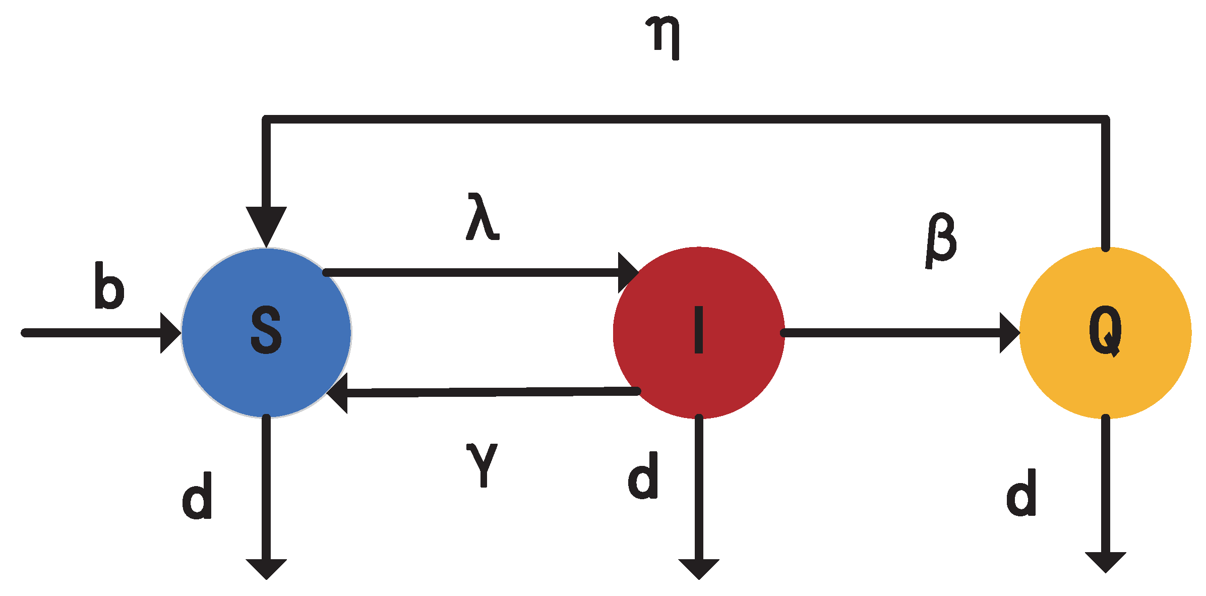
Guided by the symmetry of the contact mode on real contact networks when diseases spread, we consider a population situated on an undirected complex network N. Every node has three optional states: the susceptible state (S), quarantined state (Q), and infected state (I) [20]. We divided the population into n groups. Let , , and denote the densities of susceptible, infected, and quarantine nodes (individuals) with connectivity (degree) k at time t, respectively. The mechanism of our model mainly involves three factors. A schematic diagram is shown in Figure 1, and the meanings of the parameters are listed in Table 1. These factors are as follows:
- (1)
- Birth and death: Each vacant node i in the network randomly selects a neighbor. If the neighbor is a vacant node, the state of i remains unchanged. If the neighbor is a nonvacant node, the vacant node i will be activated to generate a new susceptible node at the birth rate b. Each nonvacant node becomes a vacant node at a natural death rate d per unit time. We assume that each nonvacant node has the same birth contact ability A (where ) due to physiological constraints.
- (2)
- Immunization and quarantine (): At each time step, susceptible individuals with degree k are immunized at the immune rate . The infected nodes with degree k will be quarantined at rate . The quarantined individuals will recover to a susceptible node at rate . Nodes with the same degree have identical quarantine and immunization strategies, while those with different degrees have different strategies.
- (3)
- SIS epidemic framework: Infection : At the initial moment, some nodes are randomly selected as infected nodes. At each time step, the possibility that each infected node i will connect to its neighboring nodes is , where represents the infectivity of infected nodes with degree k, and [38,39,40], = A [41], = [42], = [43]. If an infected node i interacts with a susceptible node j along a connecting edge, node j has a possibility of being infected by i at a transmission rate . For a node with degree k, the overall transmission rate is .
Recovery : Each infected node reverts to being susceptible at recovery rate .
According to the above assumptions, the model is as follows:
with initial conditions , , , , 2, …, n, where stands for the probability that a link which originates from a node with degree k points to an infected node. denotes the probability that a node of degree k has a reproductive contact with an individual neighbor. The denotes the possibility of selecting a neighbor with degree i of an empty node to activate it. On uncorrelated networks, the likelihood is independent of the connectedness of the originating node of the link. Thus, we note , . The average density of susceptible, infected, and quarantined nodes is , , and .
Let denote the density of individuals of degree k at time t, and We develop the equation for as
According to Ref. [44], we obtain when , and no other dynamic patterns are present; when , , where , .
Given that the original system and the limiting system exhibit identical long-term dynamic characteristics, in order to better analyze the stability of the model, we consider the limit system of (1) under the condition of and based on the analysis of . The corresponding limiting systems of model (1) are formulated as follows:
with initial conditions .
The following proposition shows that the state space of the solutions of system (3) is positively invariant.
Proposition 1.
If is a solution to system (3) that meets the initial conditions, then , and for any , i.e., Γ is positively invariant.
Proof.
∀. Thus, , and so we have .
We find that . By and Equation (2), the evolution of is derived by the following equation:
We have . Then, from system (2), we also acquire
Obviously, , and
Then, we verify for any . If not, because , there exists a and , satisfying
It is evident that for any , ; therefore, we have
Because , we obtain . On the other hand, for any , , we attain
That is to say, . When ,
Then, we acquire . It is contradictory; hence, for any k and . We also can obtain , and . That completes the proof. □
3. Equilibria and Basic Reproduction Number
In this section, the basic reproduction number is determined, which is the average number of new infections generated by a single newly infected individual throughout the entire infection period [19]. Considering the equivalent system,
Proposition 1 can show that is positively invariant for system (4). All viable steady states of system (4) satisfy the following equation:
In particular, there exists a disease-free equilibrium of (4) , and the positive equilibrium , where satisfies
The basic reproduction number can be determined according to the following theorem:
Theorem 1.
Define the basic reproduction number
There always exists a disease-free equilibrium . If and only if , the system (4) has unique positive equilibrium point , which satisfies
Proof.
Equation (6) implies that
Remark 1.
Without losing generality, we know that there always exists constant , , , , that satisfy
Then, let , we can obtain Based on [18], we can find when the network size is large enough and the second-order moment of degree ; then, can always be guaranteed to be greater than 1 and the disease will persist. Therefore, the topology of the network, such as the average degree and the second moment of degree , has an important impact on the epidemic threshold of infectious diseases.
4. Stability Analysis for SIQS Model
4.1. Stability Analysis of Disease-Free Equilibrium
Firstly, it is proved that the disease-free equilibrium (DFE) is locally asymptotically stable by the same method used in [45] by the following theorem.
Theorem 2.
Proof.
The Jacobian matrix of system (4) at is
where is the zero matrix of order n, , , is the identity matrix, and
where . Let .
Subsequently, the system (4) can be reformulated in a vector format as
Let represent a column vector and ,
The eigenvalues of matrix A are determined by . It is obvious that the characteristic equation has n multiple roots from . Other eigenvalues of matrix A are determined by . Through some elementary transformations, can be changed to
- Case 1
- If then we obtain
- Case 2
- If , since the sum of all eigenvalues is equal to the trace of the matrix, when , , and , .
Furthermore, because , we have . Since all the eigenvalues of matrix A are negative, the equilibrium point of system (4) is locally asymptotically stable when . □
Then, we get the global asymptotic stability of .
Theorem 3.
4.2. Global Stability of Endemic Equilibrium
In this section, we seek to study the conditions for the uniform persistence of disease, which is important in proving the global stability of endemic equilibrium . We obtain the uniform persistence based on Theorem 4.2 of Ref. [46]. The result of uniform persistence is shown in the following Lemma.
Lemma 1.
Proof.
Based on Theorem 4.2 of [46], we need to verify that all hypotheses for system (4) are satisfied. By setting , Condition (1) is fulfilled. Condition (2) is evidently met. For Condition (3), notice that is irreducible and whenever ; hence, there exists a positive eigenvector of , and its corresponding eigenvalue is () when , . Let ; then, we note , and it satisfies . Let ; for any , one has . Thus, Condition (3) is verified. Since every part of is negative and , Condition (4) is satisfied. To confirm Condition (5), we set . If , then
Given that every term in the above sum is non-negative, one has for all . Therefore, the only invariant set corresponding to (11) that is contained within G is . Condition (5) is satisfied. All conditions are satisfied, and the proof of uniform persistence is completed. □
From Lemma 1, it is clear that if , the infection will always exist. The following theorem shows the global stability of endemic equilibrium.
Theorem 4.
Suppose that is a solution of system (4), satisfying the initial condition. If , then , , that is to say, the endemic equilibrium is globally attractive.
Proof.
Firstly, from Lemma 1 and for any , we find that there exists such that, for t that is sufficiently large, and are satisfied. Hence, when , we obtain . Then, from system (4), we obtain
For any given constant , there exists a , when , such that
Then, from the second equation of system (4), we have
Hence, for any given constant , there exists a , such that
On the other hand, from the first equation of system (4), it can be inferred that
Hence, for any given constant , there exists a , such that,
Next, following from the second equation of system (4), we also obtain
Similarly, for any given constant , there exists a such that
Hence, , there exists a such that,
Thus,
and for any given constant , there exists a such that,
Consequently, one obtains that
Hence, for any given constant , there exists a such that
Again, one has
For any given constant , there exists a such that
It is clear that
Similarly, the calculation’s step m can be executed, resulting in four sequences. , , , are obtained as follows:
It is clear that
We find that are monotone increasing sequences and are strictly monotone decreasing sequences. It is clear that
Since all are bounded monotonic sequences, the sequential limits exist. Let
5. The Optimal Control for the SIQS Model
In this section, we study the optimal control for system (1). To meet the control objective and minimize control expenses at the same time, a viable approach to targeting epidemic outbreaks is by implementing time-varying control using optimal control theory for various infectious diseases, for example, the results in Culshaw et al. [47], Chen et al. [48], and Abboubakar et al. [49]. The aim of this section is to identify the optimal quarantine measures for controlling the transmission of diseases.
First, we introduce a time-varying control rate representing the percentage of infected individuals with degree k being quarantined. Hence, system (3) can be written as
We note the quarantine functions are bounded, Lebesgue integrable functions. Since our aim is both to reduce the scale of infection and to control its strength, we consider the following objective functional associated with the model in the control set . denotes a positive weight parameter. The objective (cost) functional is given by
In order to solve the optimal control problem, the existence of an optimal control must be assured. We applied Corollary 4.1 in Ref. [50] to prove the existence of the solution, which is shown in the proof of Theorem 5.
Theorem 5.
For the objective functional associated with model (18) defined in Ω, there exists an optimal quarantine strategy , minimizing .
Proof.
(i) Clearly, for any , the is a nonempty set of Lebesgue integrable functions. (ii) It is obvious that the solutions are bounded, ensuring the boundedness and convexity of the admissible control set. (iii) Model (18) can be written as
where is the right side of system (18), and , . It follows that
For any , since and the boundedness of the solution, there exists a constant such that . Then, there exists a positive constant M to guarantee the inequality is satisfied. (iv) Letting and , we obtain . (v) There exist , , such that .
By utilizing the results of Ref. [50], we find that there exists an optimal control , minimizing . The proof is completed. □
The solution to the optimal control problem is determined through Pontryagin’s minimum principle [50]. We note the Hamiltonian H as
If is an optimal solution of the optimal control problem, then there exists a nontrivial vector function , , satisfying the following equalities:
It follows from the derivation above that
Now the necessary conditions are implemented on the Hamiltonian H in (21) and we obtain the following results.
Theorem 6.
For a given optimal control solution and the corresponding system solution , , there is an adjacency function that satisfies the following conditions:
with conditions = = = 0. Furthermore, the optimal control is given by
Proof.
We apply the necessary conditions in the Pontryagin maximum principle with Hamiltonian function (21) to derive the adjoint variables determined by the following equations.
By the optimal conditions, we have
It follows that . Using the property of the control space, we obtain
Then, we have the optimal control in compact notation,
That completes the proof. □
6. Simulations
In this section, we conduct some numerical simulations to validate and supplement our theoretical results and to study the impact of the parameters on the dynamics of disease in order to find better control strategies. We first verify and supplement the stability results of system (1) by applying the Ode45 function in Matlab to numerically solve differential equations. It is based on the Runge Kutta method, which can efficiently solve ordinary differential equations and rigid differential equations. Next, we depict the numerical results of the optimal control problem by a combination of forward and backward difference approximation in Matlab to solve the optimal control problem. The numerical simulations include three parts. The first part is to verify the main theoretical results (Theorems 1–4) including the epidemic threshold and global stability, shown in Figure 2 and Figure 3. In the second part, we provide discussion and simulations to show the effectiveness of different immunity and quarantine strategies with degree, as shown in Figure 4 and Figure 5. The numerical simulation in the third part demonstrates the effectiveness of the optimal control method that was proven in Section 5, as shown in Figure 6 and Figure 7. We construct a BA (Barabási–Albert) scale-free network [17], which satisfies a power-law degree distribution . The network size N is set as 1000, = 80. This network evolved from the initial network with a size of , and during each time step, a new node with edges was added to the network. We note that .
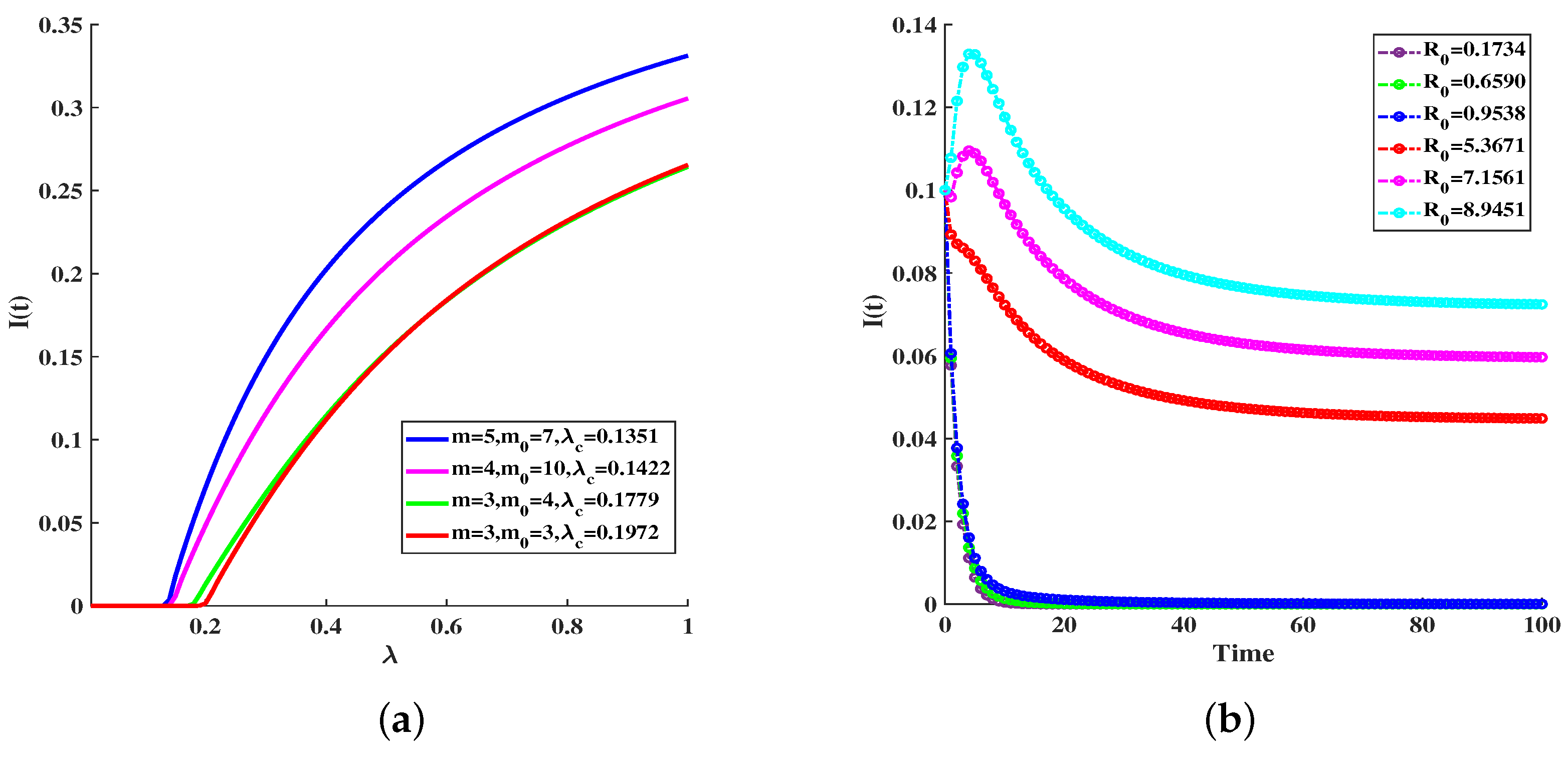
(I) Firstly, we perform some simulations in Figure 2 to verify the important results of global stability of equilibria. We denote
Figure 2a shows the relationship between and infectious rate on several different networks. Based on the basic reproduction number , we find that the epidemic threshold of the disease is , where , , , , , . One can see that the epidemic threshold is consistent with our theoretical results. Figure 2b and Table 2 verify the results of Theorems 3 and 4, i.e., if , the disease-free equilibrium is globally stable, and if , then the endemic equilibrium persists and is globally stable, where ; ; ; ; ; = 0.01, 0.038, 0.055, 0.21, 0.28, 0.35; and = 0.36, 0.36, 0.36, 0.18, 0.18, 0.18. Figure 2b shows that the disease-free equilibrium cannot undergo a Hopf bifurcation.
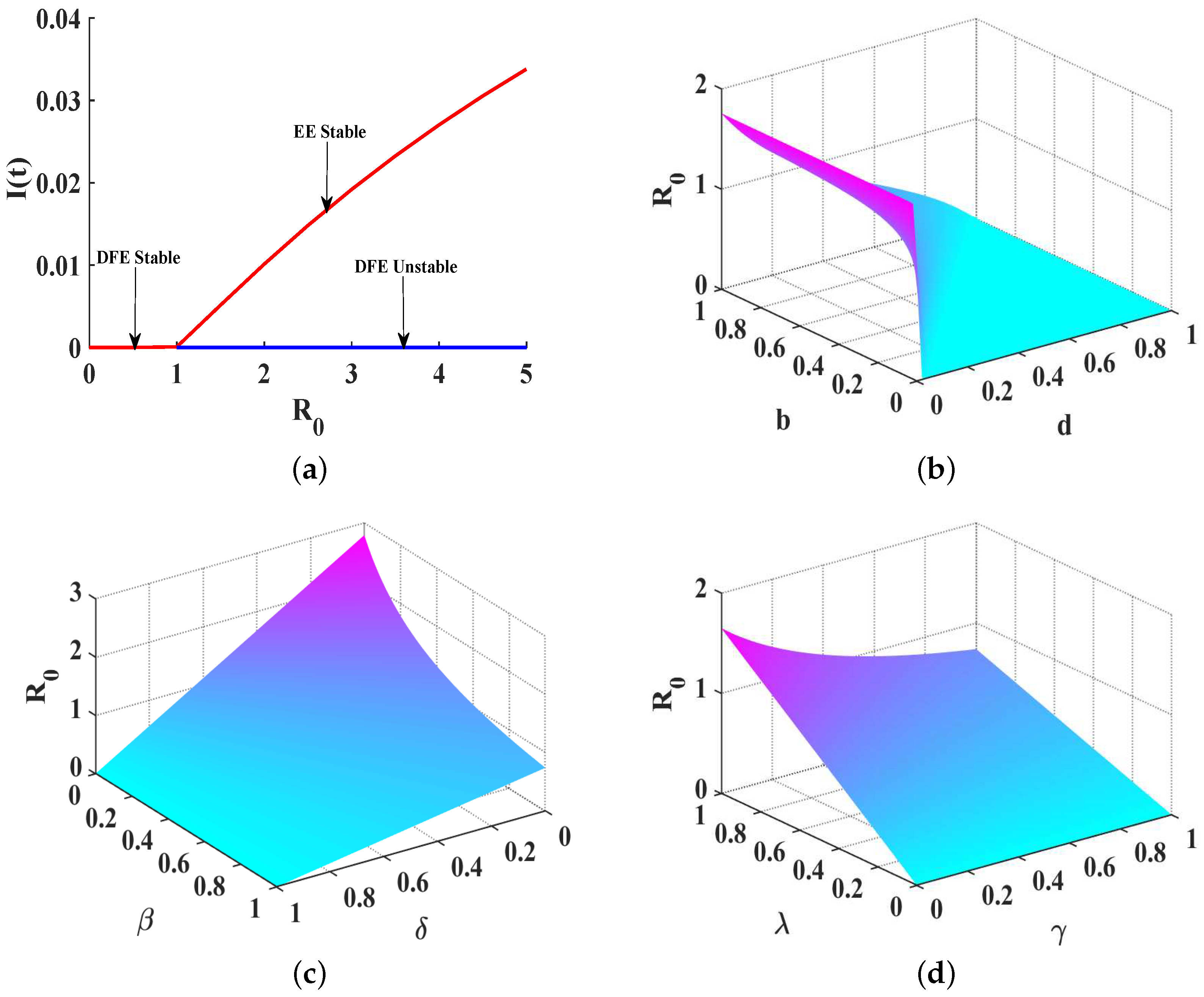
Figure 3a shows a bifurcation diagram of model system (3). It clearly appears that model system (3) exhibits a forward bifurcation, that is, the disease-free equilibrium is stable if , while if , the disease-free equilibrium is unstable, and there exists a unique endemic equilibrium which is stable. This result is consistent with the result shown in Figure 2b.
We conduct a parameter sensitivity analysis on the basic reproduction number , where
Then, let , we can obtain
This indicates that the basic reproduction number increases with the decreases in quarantine rate , immunization rate , and recovery rate , and increases with the increase in infection rate .
Without losing generality, let , . We depict the relationship between the and parameters in Figure 3b–d, which are consistent with the analysis results. Figure 3b shows that is positively correlated with the birth rate b and negatively correlated with the death rate d.
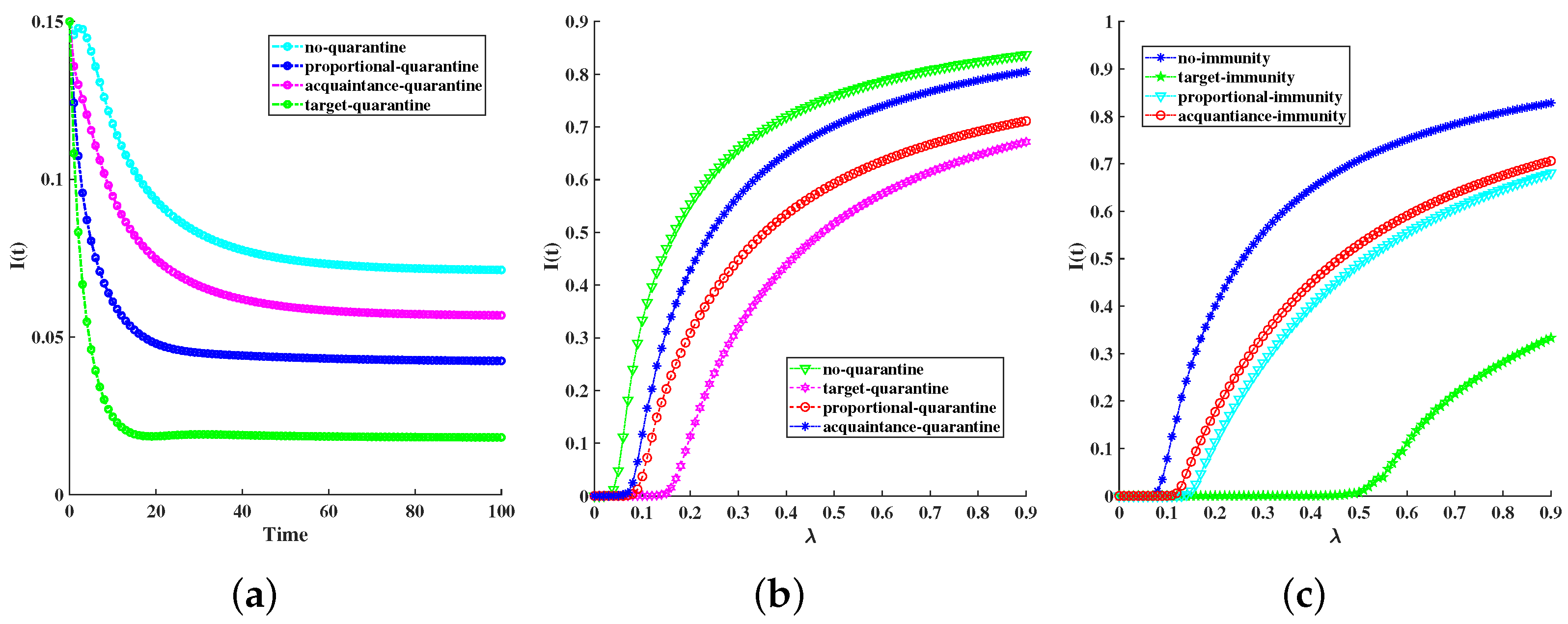
(II) Secondly, we depict the effectiveness of the immune and quarantining control strategies in Figure 4 and Figure 5. In this part, we also discuss the SIQS model (1) on the network with various immunization (proportional immunization strategy , target immunization strategy , acquaintance immunization strategy ) schemes based on [51] and define quarantine schemes of infected individuals (proportional quarantine strategy , target quarantine strategy , acquaintance quarantining strategy ) according to various immunization schemes. Then, we define the heterogeneous quarantine rate as follows:
Proportional quarantine strategy: Denote the average quarantine rate of proportional quarantine , . In randomly selecting one infected node for isolation, we find the quarantine rate is independent of the degree of the node, which is also a situation discussed in many papers.
Target quarantine strategy: We can devise a quarantine strategy for the infected nodes according to the definition of immunization [51]. Introduce an upper threshold , such that all infected nodes with connectivity are priority quarantined, i.e., we define the quarantine rate by
where , and , where is the average quarantine rate of target quarantine.
Acquaintance quarantining strategy: Select a random portion p from the N nodes. The likelihood of quarantining an infected node with degree k is given by ; therefore, . We note that denotes the average quarantine rate of acquaintance quarantine, where .
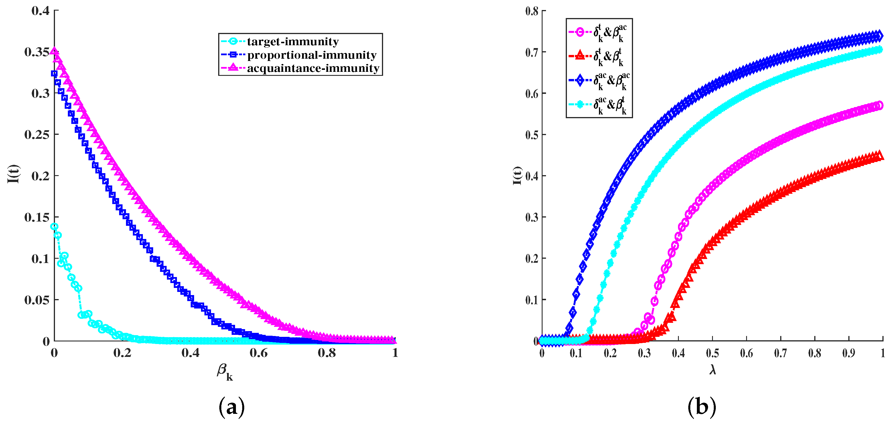
Figure 4a shows the under different quarantining control strategies; the target quarantine strategy is the most effective in controlling disease. Figure 4b compares the effectiveness of different quarantine strategies. From Figure 4a,b and Table 3, we find that the target quarantine strategy has better effectiveness than others. Figure 4c shows the effectiveness of different immunity strategies; it shows that all three immunization schemes are effective compared to the case without any immunization, and the targeted immunization scheme is more efficient than the proportional scheme discussed.
Figure 5a depicts the average infectious density with respect to quarantine rate under different immunity strategies. It also shows that the target strategy is better than the proportional and acquaintance strategies. We further show the average infectious density with respect to infected rate for the target and acquaintance immunization schemes and quarantine strategies in Figure 5b. We find that the targeted immunity and the target quarantine strategy have better effectiveness than others.
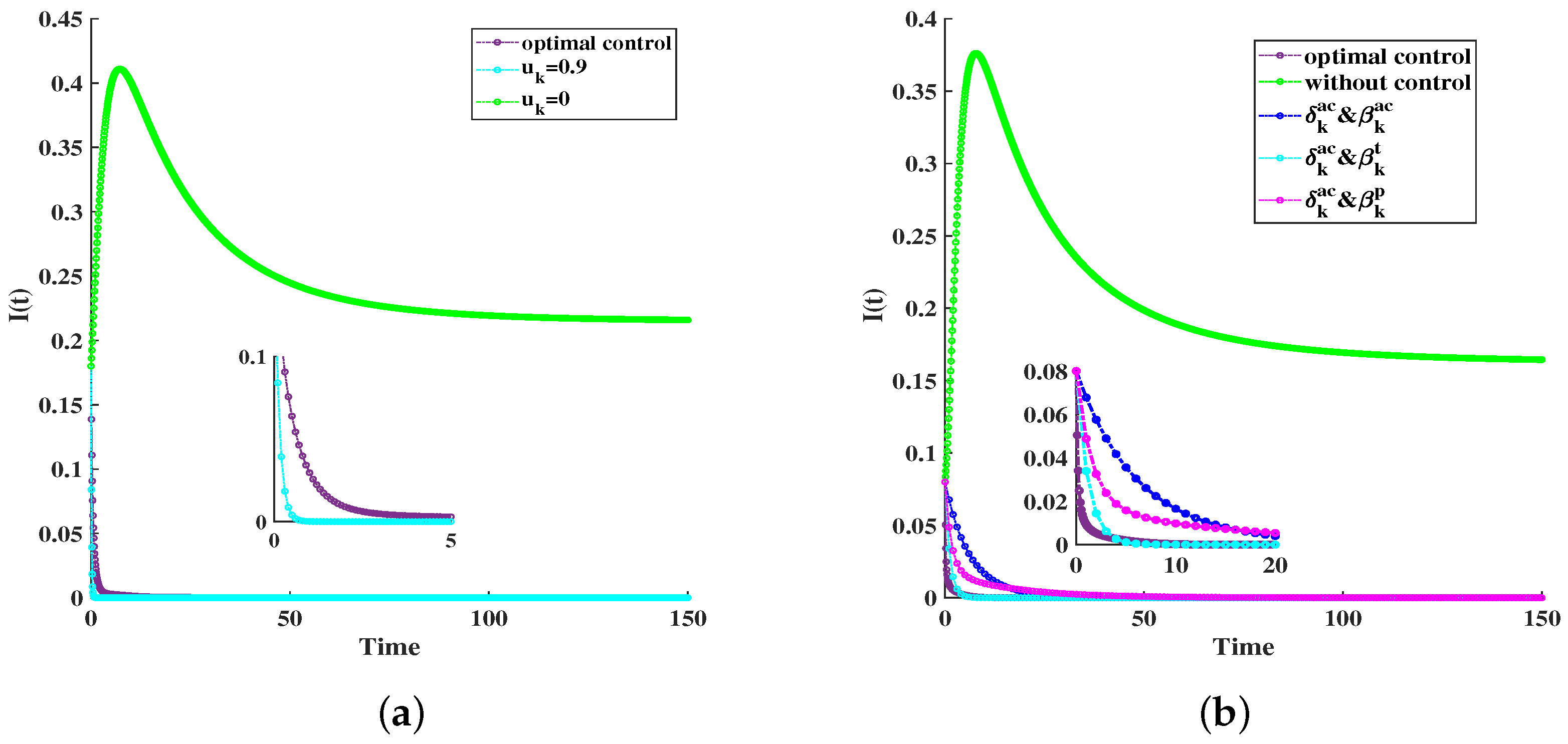
(III) Thirdly, we analyze and illustrate the optimal control and various quarantine schemes by numerical simulations, as shown in Figure 6 and Figure 7. In Figure 6, we depict under different control strategies. In order to provide a clearer representation of the findings in Figure 6a, we additionally compute the objective function values for diverse control approaches, as shown in Table 4. In the absence of any control strategy (i.e., ), the infection ultimately breaks out and reaches a stable level of infection. We also set a fixed control strategy compared with the optimal control strategy, finding that if we want to obtain better results than the optimal control strategy, it will usually lead to a significant increase in control costs (i.e., ). In Figure 6b, we compare, the effects of optimal control, without control, and acquaintance immunity, combining these with multiple quarantine strategies for infectious disease control. Compared with other strategies, the optimal control strategy has the best control effect.
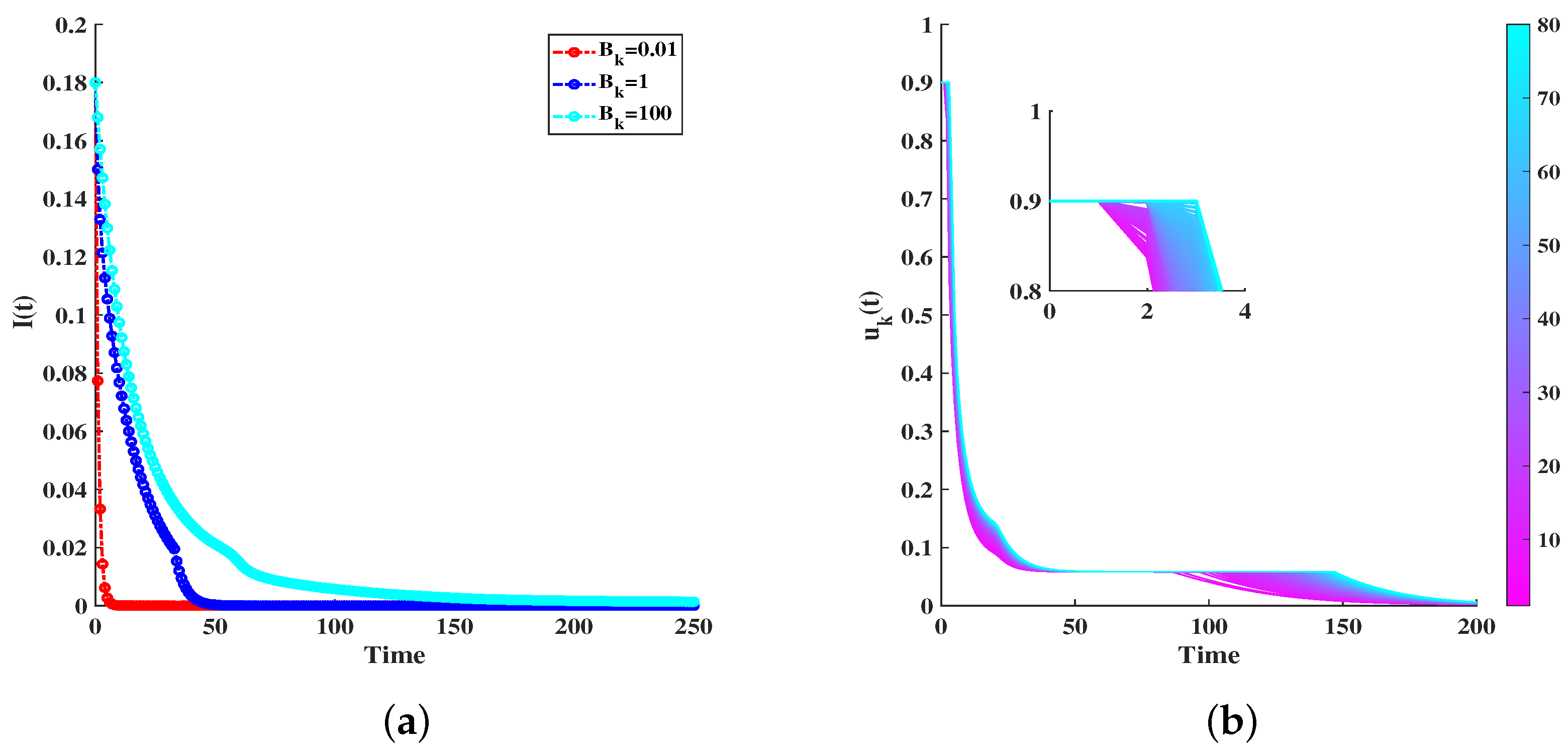
Figure 7a illustrates the under optimal control under three cases: low cost at , moderate cost at , and high cost at . Even under high costs, as seen in the third scenario, the scale of infection can be notably curtailed through optimal control. Figure 7b displays the fluctuation of across varying degrees under optimal regulation. It is evident that tends to escalate as the degree rises. It indicates a higher level of infection, resulting in a higher value of .
7. Conclusions
We proposed an SIQS epidemic model with heterogeneous immune and quarantine measures on heterogeneous networks. We performed a detailed mathematical analysis of our system, which showed that the basic reproduction number is collectively determined by the infection rate and the effectiveness of disease control measures. Specifically, when , the disease-free equilibrium exhibits global asymptotic stability. When , the endemic equilibrium demonstrates both local and global asymptotic stability. At the same time, we conducted an in-depth theoretical examination of system (1) to tackle the optimal quarantine control issue, confirming the presence of optimal solutions. We hope this result can provide some ideas for solving the optimal solution of asymmetric quarantine strategies on heterogeneous networks. We defined different forms of quarantine measures, which are asymmetric quarantine strategies related in degree, and numerically simulated the effectiveness of a combination of different quarantine strategies and immune schemes in controlling diseases. Our findings indicate that the implementation of any control strategy can have a favorable impact on the magnitude of an epidemic outbreak, with the optimal control being particularly effective. Among them, the effect of a target quarantine scheme can be comparable to the effect of optimal control. However, target isolation requires knowing the degree of all nodes in the network, which has a significant cost and workload. Therefore, in order to achieve the control goal and reduce the control cost at the same time, the optimal control strategy considering the asymmetry of control measures related in degree and time is shown to be superior to the symmetric control strategies.
A variety of control strategies, such as quarantine and immune schemes, can be employed for the effective management, mitigation, and potential eradication of infectious diseases. This paper can contribute to an understanding of the dynamics of infectious disease with control measures. However, our paper is not based on a specific infectious disease, so there are still certain limitations in providing a specific basis for public health prevention measures. Studying the control measures for a specific disease based on disease data will be meaningful work.
Author Contributions
Conceptualization, S.C. and K.-K.S.; methodology, S.C., Y.W. and L.L.; software, S.C., Y.W. and L.L.; validation, S.C. and Y.W.; formal analysis, S.C. and K.-K.S.; writing—original draft preparation, Y.W. and S.C.; writing—review and editing, Y.W., S.C., D.Y. and K.-K.S.; visualization, Y.W., S.C. and K.-K.S.; supervision, K.-K.S.; funding acquisition, D.Y. All authors have read and agreed to the published version of the manuscript.
Funding
This work is supported by the National Social Science Funds of China (Grant No. 22BSH025), National Natural Science Foundation of China (Grant No. 62303303 and Grant No. 61803047), Major Project of The National Social Science Foundation of China (19ZDA149, 19ZDA324), and Fundamental Research Funds for the Central Universities (14370119, 14390110). Ke-Ke Shang is supported by the Jiangsu Qing Lan Project.
Data Availability Statement
No new data were created in this study. Data sharing is not applicable to this article.
Acknowledgments
We acknowledge the Theoretical Physics of Complex Systems Center (Nanjing University). We are deeply grateful to Jack Murdoch Moore, a native English speaker, for his significant contributions in revising and enhancing our paper. His Google Scholar profile: https://scholar.google.com/citations?user=AFDBPpYAAAAJ&hl=en (accessed on 26 January 2024). His personal website: https://jackmurdochmoore.github.io/JackMurdochMoore/ (accessed on 26 January 2024).
Conflicts of Interest
The authors declare no conflicts of interest.
References
- Yang, B.; Shang, K.K.; Michael, S.; Chao, N.P. Information overload: How hot topics distract from news—COVID-19 spread in the US. Natl. Sci. Open 2023, 2, 20220051. [Google Scholar] [CrossRef]
- Jose, S.A.; Raja, R.; Omede, B.; Agarwal, R.P.; Alzabut, J.; Cao, J.; Balas, V. Mathematical modeling on co-infection: Transmission dynamics of Zika virus and Dengue fever. Nonlinear Dyn. 2023, 111, 4879–4914. [Google Scholar] [CrossRef]
- Peter, O.J.; Afolabi, O.A.; Victor, A.A.; Akpan, C.E.; Oguntolu, F.A. Mathematical model for the control of measles. J. Appl. Sci. Environ. Manag. 2018, 22, 571–576. [Google Scholar] [CrossRef]
- Fraser, C.; Donnelly, C.A.; Cauchemez, S.; Hanage, W.P.; Van Kerkhove, M.D.; Hollingsworth, T.D.; Griffin, J.; Baggaley, R.F.; Jenkins, H.E.; Lyons, E.J.; et al. Pandemic potential of a strain of influenza A (H1N1): Early findings. Science 2009, 324, 1557–1561. [Google Scholar] [CrossRef]
- Lipsitch, M.; Cohen, T.; Cooper, B.; Robins, J.M.; Ma, S.; James, L.; Gopalakrishna, G.; Chew, S.K.; Tan, C.C.; Samore, M.H.; et al. Transmission dynamics and control of severe acute respiratory syndrome. Science 2003, 300, 1966–1970. [Google Scholar] [CrossRef] [PubMed]
- Cai, L.M.; Li, Z.Q.; Song, X.Y. Global analysis of an epidemic model with vaccination. J. Appl. Math. Comput. 2018, 57, 605–628. [Google Scholar] [CrossRef] [PubMed]
- Kermack, W.O.; McKendrick, A.G. A contribution to the mathematical theory of epidemics. Proc. R. Soc. Lond. Ser. Contain. Pap. Math. Phys. Character 1927, 115, 700–721. [Google Scholar]
- Kermack, W.O.; McKendrick, A.G. Contributions to the mathematical theory of epidemics. II.The problem of endemicity. Proc. R. Soc. Lond. Ser. Contain. Pap. Math. Phys. Character 1932, 138, 55–83. [Google Scholar]
- Kermack, W.O.; McKendrick, A.G. Contributions to the mathematical theory of epidemics. III.Further studies of the problem of endemicity. Proc. R. Soc. Lond. Ser. Contain. Pap. Math. Phys. Character 1933, 141, 94–122. [Google Scholar]
- Chen, S.S.; Small, M.; Fu, X.C. Global stability of epidemic models with imperfect vaccination and quarantine on scale-free networks. IEEE Trans. Netw. Sci. Eng. 2019, 7, 1583–1596. [Google Scholar] [CrossRef]
- Peter, O.J.; Adebisi, A.F.; Ajisope, M.O.; Ajibade, F.O.; Abioye, A.I.; Oguntolu, F.A. Global stability analysis of typhoid fever model. Adv. Syst. Sci. Appl. 2020, 20, 20–31. [Google Scholar]
- Jose, S.A.; Raja, R.; Dianavinnarasi, J.; Baleanu, D.; Jirawattanapanit, A. Mathematical modeling of chickenpox in Phuket: Efficacy of precautionary measures and bifurcation analysis. Biomed. Signal Process. Control 2023, 84, 104714. [Google Scholar] [CrossRef]
- Hethcote, H.; Zhi En, M.; Sheng Bing, L. Effects of quarantine in six endemic models for infectious diseases. Math. Biosci. 2002, 180, 141–160. [Google Scholar] [CrossRef] [PubMed]
- Suo, Y.H. Asymptotical Stability of an SIQS Epidemic Model with Age Dependence and Generally Nonlinear Contact Rate. Appl. Mech. Mater. 2011, 58, 292–297. [Google Scholar] [CrossRef]
- Wei, F.Y.; Chen, F.X. Stochastic permanence of an SIQS epidemic model with saturated incidence and independent random perturbations. Phys. A Stat. Mech. Its Appl. 2016, 453, 99–107. [Google Scholar] [CrossRef]
- Zhang, X.B.; Liu, R.J. The stationary distribution of a stochastic SIQS epidemic model with varying total population size. Appl. Math. Lett. 2021, 116, 106974. [Google Scholar] [CrossRef]
- Barabási, A.L.; Albert, R. Emergence of scaling in random networks. Science 1999, 509–512, 286. [Google Scholar] [CrossRef]
- Pastor-Satorras, R.; Vespignani, A. Epidemic dynamics and endemic states in complex networks. Phys. Rev. E 2001, 63, 066117. [Google Scholar] [CrossRef]
- Cheng, X.X.; Wang, Y.; Huang, G. Global dynamics of a network-based SIQS epidemic model with nonmonotone incidence rate. Chaos Solitons Fractals 2021, 153, 111502. [Google Scholar] [CrossRef]
- Zhao, R.D.; Liu, Q.M.; Sun, M.C. Dynamical behavior of a stochastic SIQS epidemic model on scale-free networks. J. Appl. Math. Comput. 2022, 68, 813–838. [Google Scholar] [CrossRef]
- Li, T.; Wang, Y.M.; Guan, Z.H. Spreading dynamics of a SIQRS epidemic model on scale-free networks. Commun. Nonlinear Sci. Numer. Simul. 2014, 19, 686–692. [Google Scholar] [CrossRef]
- Kang, H.Y.; Liu, K.H.; Fu, X.C. Dynamics of an epidemic model with quarantine on scale-free networks. Phys. Lett. A 2017, 381, 3945–3951. [Google Scholar] [CrossRef]
- Wang, H.Y.; Moore, J.M.; Small, M.; Wang, J.; Yang, H.; Gu, C. Epidemic dynamics on higher-dimensional small world networks. Appl. Math. Comput. 2022, 421, 126911. [Google Scholar] [CrossRef]
- Iacoviello, D.; Stasio, N. Optimal control for SIRC epidemic outbreak. Comput. Methods Programs Biomed. 2013, 110, 333–342. [Google Scholar] [CrossRef]
- Buonomo, B.; Lacitignola, D.; Vargas-De-León, C. Qualitative analysis and optimal control of an epidemic model with vaccination and treatment. Math. Comput. Simul. 2014, 100, 88–102. [Google Scholar] [CrossRef]
- Kandhway, K.; Kuri, J. How to run a campaign: Optimal control of SIS and SIR information epidemics. Appl. Math. Comput. 2014, 231, 79–92. [Google Scholar] [CrossRef]
- Kandhway, K.; Kuri, J. Optimal control of information epidemics modeled as Maki Thompson rumors. Commun. Nonlinear Sci. Numer. Simul. 2014, 19, 4135–4147. [Google Scholar] [CrossRef]
- Jang, J.; Kwon, H.D.; Lee, J. Optimal control problem of an SIR reaction–diffusion model with inequality constraints. Math. Comput. Simul. 2020, 171, 136–151. [Google Scholar] [CrossRef]
- Wang, B.; Tian, X.H.; Xu, R.; Song, C.W. Threshold dynamics and optimal control of a dengue epidemic model with time delay and saturated incidence. J. Appl. Math. Comput. 2023, 69, 871–893. [Google Scholar] [CrossRef]
- Chen, L.J.; Sun, J.T. Global stability and optimal control of an SIRS epidemic model on heterogeneous networks. Phys. A Stat. Mech. Its Appl. 2014, 410, 196–204. [Google Scholar] [CrossRef]
- Chen, L.J.; Sun, J.T. Optimal vaccination and treatment of an epidemic network model. Phys. Lett. A 2014, 378, 3028–3036. [Google Scholar] [CrossRef]
- Xu, D.G.; Xu, X.Y.; Xie, Y.F.; Yang, C.H. Optimal control of an SIVRS epidemic spreading model with virus variation based on complex networks. Commun. Nonlinear Sci. Numer. Simul. 2017, 48, 200–210. [Google Scholar] [CrossRef]
- Jia, N.; Ding, L.; Liu, Y.J.; Hu, P. Global stability and optimal control of epidemic spreading on multiplex networks with nonlinear mutual interaction. Phys. A Stat. Mech. Its Appl. 2018, 502, 93–105. [Google Scholar] [CrossRef]
- Li, K.Z.; Zhu, G.H.; Ma, Z.J.; Chen, L.J. Dynamic stability of an SIQS epidemic network and its optimal control. Commun. Nonlinear Sci. Numer. Simul. 2019, 66, 84–95. [Google Scholar] [CrossRef]
- Wei, X.D.; Xu, G.C.; Zhou, W.S. Global stability of endemic equilibrium for a SIQRS epidemic model on complex networks. Phys. A Stat. Mech. Its Appl. 2018, 512, 203–214. [Google Scholar] [CrossRef]
- Zhang, L.; Liu, M.X.; Xie, B.L. Optimal control of an SIQRS epidemic model with three measures on networks. Nonlinear Dyn. 2021, 103, 2097–2107. [Google Scholar] [CrossRef]
- Yang, P.; Jia, J.B.; Shi, W.; Feng, J.W.; Fu, X.C. Stability analysis and optimal control in an epidemic model on directed complex networks with nonlinear incidence. Commun. Nonlinear Sci. Numer. Simul. 2023, 121, 107206. [Google Scholar] [CrossRef]
- Pastor-Satorras, R.; Vespignani, A. Epidemic dynamics in finite size scale-free networks. Phys. Rev. E 2002, 65, 035108. [Google Scholar] [CrossRef]
- Moreno, Y.; Pastor-Satorras, R.; Vespignani, A. Epidemic outbreaks in complex heterogeneous networks. Eur. Phys. J.-Condens. Matter Complex Syst. 2002, 26, 521–529. [Google Scholar] [CrossRef]
- Wang, L.; Dai, G.Z. Global stability of virus spreading in complex heterogeneous networks. SIAM J. Appl. Math. 2008, 68, 1495–1502. [Google Scholar] [CrossRef]
- Yang, R.; Wang, B.H.; Ren, J.; Bai, W.J.; Shi, Z.W.; Wang, W.X.; Zhou, T. Epidemic spreading on heterogeneous networks with identical infectivity. Phys. Lett. A 2007, 364, 189–193. [Google Scholar] [CrossRef]
- Chu, X.W.; Zhang, Z.Z.; Guan, J.H.; Zhou, S.G. Epidemic spreading with nonlinear infectivity in weighted scale-free networks. Phys. A Stat. Mech. Its Appl. 2011, 390, 471–481. [Google Scholar] [CrossRef]
- Zhang, H.F.; Fu, X.C. Spreading of epidemics on scale-free networks with nonlinear infectivity. Nonlinear Anal. Theory Methods Appl. 2009, 70, 3273–3278. [Google Scholar] [CrossRef]
- Zhu, G.H.; Chen, G.R.; Xu, X.J.; Fu, X.C. Epidemic spreading on contact networks with adaptive weights. J. Theor. Biol. 2013, 317, 133–139. [Google Scholar] [CrossRef] [PubMed]
- Liu, X.N.; Takeuchi, Y.; Iwami, S. SVIR epidemic models with vaccination strategies. J. Theor. Biol. 2008, 253, 1–11. [Google Scholar] [CrossRef] [PubMed]
- Lajmanovich, A.; Yorke, J.A. A deterministic model for gonorrhea in a nonhomogeneous population. Math. Biosci. 1976, 28, 221–236. [Google Scholar] [CrossRef]
- Culshaw, R.V.; Ruan, S.; Spiteri, R.J. Optimal HIV treatment by maximising immune response. J. Math. Biol. 2004, 48, 545–562. [Google Scholar] [CrossRef] [PubMed]
- Chen, P.Y.; Cheng, S.M.; Chen, K.C. Optimal control of epidemic information dissemination over networks. IEEE Trans. Cybern. 2014, 44, 2316–2328. [Google Scholar] [CrossRef]
- Abboubakar, H.; Guidzavai, A.K.; Yangla, J.; Damakoa, I.; Mouangue, R. Mathematical modeling and projections of a vector-borne disease with optimal control strategies: A case study of the Chikungunya in Chad. Chaos Solitons Fractals 2021, 150, 111197. [Google Scholar] [CrossRef]
- Fleming, W.; Rishel, R. Deterministic and Stochastic Optimal Control; Springer: Berlin/Heidelberg, Germany, 1975; p. 222. [Google Scholar]
- Fu, X.C.; Small, M.; Walker, D.M.; Zhang, H.F. Epidemic dynamics on scale-free networks with piecewise linear infectivity and immunization. Phys. Rev. E 2008, 77, 036113. [Google Scholar] [CrossRef]
Figure 1.
The block diagram of the SIQS model. Here S, I, and Q represent susceptible, infected, and quarantined states.
Figure 1.
The block diagram of the SIQS model. Here S, I, and Q represent susceptible, infected, and quarantined states.

Figure 2.
(a) The with respect to and the structure of a network with different parameters m and . denotes the theoretical epidemic threshold. Other parameter settings are as follows: , , , , , . (b) The average infected density under different parameters: 0.01, 0.038, 0.055, 0.21, 0.28, 0.3; = 0.36, 0.36, 0.36, 0.18, 0.18, 0.18; ; ; ; ; and , which correspond to = 0.1734, 0.6590, 0.9538 < 1; = 5.3671, 7.1561, 8.9451 > 1.

Figure 3.
(a) Bifurcation diagram of model system (1). EE is the endemic equilibrium , DFE is the disease-free equilibrium : , , , , , . (b–d) The combined influence of parameters on . (b) The relationship between and b, d: , , , , . (c) The relationship between and , : , , , , . (d) The relationship between and ,: , , , , .

Figure 4.
(a) under different quarantining control strategies: no quarantine (cyan line), acquaintance quarantine (magenta line), proportional quarantine (blue line), target quarantine (green line): , , , , , (b) The epidemic threshold under different quarantine control strategies: no quarantine (green line), target quarantine (magenta line), acquaintance quarantine (blue line), proportional quarantine (red line): , , , , , , , . (c) The epidemic threshold under different immunization strategies: no immunity (blue line), target immunity (green line), proportional immunity (cyan line), acquaintance immunity (red line): , , , , , , , , .

Figure 5.
The effectiveness of combination immunization and quarantine control strategies: , , , , , . (a) Different immunization strategies with respect to quarantine rate: , , ; acquaintance immunization (magenta line), proportional immunization (blue line), target immunization (cyan line). (b) Comparison of different combination control strategies: , , , , , ; target immunization and target quarantine (red line); target immunization and acquaintance quarantine (magenta line); acquaintance immunization and target quarantine (cyan line); acquaintance immunization and acquaintance quarantine (blue line).

Figure 6.
(a) The average density under different control strategies. The lines with different colors correspond to different optimal control strategies: optimal control (purple line); (cyan line); (green line). Other parameter settings are as follows: , , , , , . (b) Comparison of optimal control and combined heterogeneous control strategies, without control (green line); acquaintance immunization and acquaintance quarantine (blue line); acquaintance immunization and proportional quarantine (magenta line); acquaintance immunization and target quarantine (cyan line); optimal control (purple line): , , , , , , , , .

Figure 7.
(a) under optimal control with varying weights. Low costs: (red line); moderate costs: (blue line); high costs: (cyan line). Other parameters are fixed as , , , , , . (b) The quarantine rates for any degree. Other parameters are fixed as , , , , , .
Figure 7.
(a) under optimal control with varying weights. Low costs: (red line); moderate costs: (blue line); high costs: (cyan line). Other parameters are fixed as , , , , , . (b) The quarantine rates for any degree. Other parameters are fixed as , , , , , .


Table 1.
Symbols employed in models.
| Symbols | Description |
|---|---|
| Proportion of nodes with degree k. | |
| Average degree . | |
| n | Maximum degree. |
| b | Birth rate. |
| d | Natural death rate. |
| Fertile contact probability between a node with degree k and its neighbors. | |
| Transmission rate of infected nodes with degree k. | |
| Vaccination rate of susceptible nodes with degree k. | |
| Quarantine rate of infected nodes with degree k. | |
| Recovery rate of infected nodes. | |
| Recovery rate of quarantined nodes. |
Table 2.
Final infection scale under different in Figure 2b.
Table 2.
Final infection scale under different in Figure 2b.
| Basic reproduction number | 0.1734 | 0.6590 | 0.9538 | 5.3671 | 7.1561 | 8.9451 |
| Final infection scale | 0 | 0 | 0 | 0.0449 | 0.0597 | 0.0724 |
Table 3.
Final infection scale and under different control strategies in Figure 4a,b.
Table 3.
Final infection scale and under different control strategies in Figure 4a,b.
| Quarantining Control Strategies | Final Infection Scale | Epidemic Threshold |
|---|---|---|
| No quarantine | 0.0713 | 0.0468 |
| Acquaintance quarantine | 0.0568 | 0.0724 |
| Proportional quarantine | 0.0424 | 0.0798 |
| Target quarantine | 0.0182 | 0.1483 |
Table 4.
The values of under different control strategies.
| Optimal Control | Max Control | No Control |
|---|---|---|
Disclaimer/Publisher’s Note: The statements, opinions and data contained in all publications are solely those of the individual author(s) and contributor(s) and not of MDPI and/or the editor(s). MDPI and/or the editor(s) disclaim responsibility for any injury to people or property resulting from any ideas, methods, instructions or products referred to in the content. |
© 2024 by the authors. Licensee MDPI, Basel, Switzerland. This article is an open access article distributed under the terms and conditions of the Creative Commons Attribution (CC BY) license (https://creativecommons.org/licenses/by/4.0/).
Share and Cite
MDPI and ACS Style
Wang, Y.; Chen, S.; Yu, D.; Liu, L.; Shang, K.-K. Propagation Dynamics of an Epidemic Model with Heterogeneous Control Strategies on Complex Networks. Symmetry 2024, 16, 166. https://doi.org/10.3390/sym16020166
AMA Style
Wang Y, Chen S, Yu D, Liu L, Shang K-K. Propagation Dynamics of an Epidemic Model with Heterogeneous Control Strategies on Complex Networks. Symmetry. 2024; 16(2):166. https://doi.org/10.3390/sym16020166
Chicago/Turabian StyleWang, Yan, Shanshan Chen, Dingguo Yu, Lixiang Liu, and Ke-Ke Shang. 2024. "Propagation Dynamics of an Epidemic Model with Heterogeneous Control Strategies on Complex Networks" Symmetry 16, no. 2: 166. https://doi.org/10.3390/sym16020166
Note that from the first issue of 2016, this journal uses article numbers instead of page numbers. See further details here.