Attack–Defense Confrontation Analysis and Optimal Defense Strategy Selection Using Hybrid Game Theoretic Methods

Abstract

False data injection attacks are executed in the electricity markets of smart grid systems for financial benefits. The attackers can maximize their profits through modifying the estimated transmission power and changing the prices of market electricity. As a response, defenders need to minimize expected load losses and generator trips through load and power generation adjustments. The selection of strategies of the attacking and defending sides turns out to be a symmetric game process. This article proposes a hybrid game theory method for analyzing the attack–defense confrontation: firstly, a micro-grid-based power market model considering false data injection attacks is established using the Nash equilibrium method; secondly, the attack–defense game function is constructed and solved via the Stackelberg equilibrium algorithm. The Markov game algorithm and distributed learning algorithm are used to update equilibrium function; finally, a dynamic game behavior model of the two players is constructed through simulating the attack–defense probability. The evolutionary game method is used to select the optimal defense strategy for dynamic probability changes. Modified IEEE standard bus systems are illustrated to certify the effectiveness of the proposed model.

1. Introduction

Recently, smart grid (SG) systems with networking characteristics and uncertainty distributed power supplies have become increasingly complex [1]. Cyber-attack problems have become the main security issue for the reliability and security of SG operation [2]. False data injection (FDI) attacks are able to bypass the online monitoring of state estimation, steal energy, and gain economic benefits through false scheduling [3]. Attackers establish their own behavior through monitoring and injecting attacks, which may interfere with operations and modify estimated transmission power [4]. The payoff function is established to maximize their economic benefit with the least attack cost [5]. Meanwhile, the defenders of the system need to establish corresponding multi-level defense measures to deal with attacks and mitigate risks. The payoff function of defenders is established to minimize expected load losses and generator trips based on the current attack situations [6]. The selection of strategies by the attackers and defenders whose motives and emergency responses are contradictory can be modeled with a symmetric game process [7]. The game method is constructed to admit equilibrium to enable the two players to maximize their respective minimum rewards [8].

Relying on the ability to make multifaceted decisions on power grid security issues, game theory is widely applied in the field of network security [9,10,11,12,13,14,15,16]. In [9], a security resource allocation game model is established to discuss the load redistribution attacks problem. Both system operators and attackers maximize their own payoffs through selecting the optimal strategy; in [10], the game composed of attackers and defenders is constructed with a probability-weighting algorithm, and the optimal investment strategies of the players are obtained using the Nash Equilibrium. However, refs. [9,10] are inadequate in describing how both offensive and defensive strategies change with each other; ref. [11] investigates the Stackelberg game through having legitimate launchers act as leaders, and disruptors acting as followers. A genetic algorithm was used to obtain the optimal frequency hopping speed and optimal transmission power; ref. [12] formulates a Stackelberg game model through making the Cloud provider the leader and making attackers the second player, and obtains the utility function through applying artificial neural networks. Refs. [11,12] establish the master–slave change of offensive and defensive strategies. However, the model lacks in describing the cumulative profits in a dynamic, changing game process; ref. [13] establishes a Markov anti-attack model, compares the effectiveness of network space simulation defense under different attack types, and uses dynamic games with incomplete information to determine the optimal strategy; ref. [14] formulates a multistage optimization model for the deployment of a mobile target defense mechanism under a Markov decision, maximizing the profits under environmental constraints. However, each iteration solution of [13,14] depends on the revenue in the current unit time, ignoring the previous revenue, bringing in an exponential increase in complex calculations; in [15], a Markovian–Stackelberg game is proposed to simulate the sequential actions of attackers and defenders, and a secure constrained optimal power flow is given, which preserves the safety margin of key components to minimize the power outage scale and potential future risks; in [16], the adversarial interaction of the attacker and defender is modeled as a resource-constrained game, and a linear-time algorithm is used to obtain the optimal defense strategy. However, the game process in the above works assumes that both sides (attacker and defender) of the game are in pure rationality. In practice, the players will constantly adjust their strategies and dynamically pursue profits. Therefore, common rational game models overlook the limitations of bounded rationality, which can lead to deviations between attack and defense behaviors and actual situations, thereby weakening the accuracy and guiding value of security defense strategy selection methods. Regarding the above problem, evolutionary game method [17] is put in to analyze the ability of limited rationality in offensive and defensive behavior. The evolutionary game takes bounded rational players as the basis of game analysis. Based on the idea of biological dynamic evolution, it depicts both sides of attack and defense through a learning mechanism, and constantly improves the internal drive of behavior strategy [18,19]. The evolutionary game in the above works has established the evolutionary game between attackers and defenders according to system dynamics. The goal of optimal overall network performance is achieved. However, the method of solving evolutionary game equilibrium and the specific strategy selection method are not designed, which makes it difficult to guide the security defense decision.

Therefore, in view of the selection of the security defense strategy in network attack–defense confrontation, this paper analyzes the evolutionary trend of offensive and defensive behavior from limited rationality in reality. On this basis, the evolutionary stability strategy solution method is proposed to achieve the selection of optimal defense strategies. At the same time, low-income players in the game process are constantly learning from the strategies of the high-income players. This reflects the dynamic evolutionary trend of offensive and defensive confrontation under bounded rationality constraints. In addition, the law of forming an evolutionary stable equilibrium in different situations is also analyzed and summarized.

Further, this article considers the impact of the optimized output of micro-grid (MG) energy management on the dynamic strategy selection of two participants. The MG combines distributed energy, storage devices, and corresponding loads in a reduced space through advanced control systems [20]. The MG can participate in the electricity market through online trading with the main power grid, and can also operate independently in island mode to balance internal supply and demand [21,22]. The MG has played an increasingly important role in maintaining the power balance of the entire SG power system and reducing generation costs. The optimal operation results of the electricity market and generation output are considered in the game equilibrium solution.

The main contributions of this paper are listed as follows:

(1)

MG-based electricity markets model of an SG power system is considered for FDI attacks. The electricity market is established with a double-sided bidding mechanism using the Nash equilibrium game theory.

(2)

A hybrid game model of payoff function between attack and defense is established. Game theoretic methods are proposed to discuss the interaction behavior between attack and defense sides.

(3)

The benefits according to attack and defense strategies are quantified using the evolutionary game method, and the dynamic evolutionary learning of attack and defense probability is discussed.

(4)

The optimal defense strategy is selected after the evolutionary stable equilibrium solution is solved, and the dynamic confrontation trend of both sides is studied.

This article proposes a hybrid game theory method for analyzing the attack–defense confrontation: firstly, a micro-grid-based power market model considering false data injection attacks is established using the Nash equilibrium method; secondly, the attack–defense game function is constructed and solved via the Stackelberg equilibrium algorithm. The Markov game algorithm and distributed learning algorithm are used to update equilibrium function; finally, a dynamic game behavior model of the two players is constructed through simulating the attack–defense probability. The evolutionary game method is used to select the optimal defense strategy for dynamic probability changes.

The rest of this paper is organized as follows: The power market attack model with micro-grid participation is provided in Section 2; in Section 3, the game model of payoff function between attack and defense is established. Game theoretic methods are proposed to discuss the interaction behavior between the attacking and defending sides. An attack–defense evolutionary game model is constructed to obtain optimal strategies against the dynamic changing probability in Section 4. The optimal selection strategies for the defender are also listed in this section; numerical examples and discussions of the modified IEEE standards for 14 bus systems and 118 bus systems are presented in Section 5; the concluding remarks and future works are submitted in Section 6.

2. Electricity Markets Attack Model

In an electricity power market, the net power injection is expressed as the difference between generation and load. The state variable $x$ is expressed by the relationship between power generation vector $P$ and demand vector $L$ as below.

$$x={\left[L^T,P^T\right]}^T$$

(1)

Then the line flow vector $F$ will be expressed as below.

$$F=H_{f}x=H_f{\left[L^T,P^T\right]}^T$$

(2)

$H_f$ is the measurement matrix of the distribution factor for the transmission line flow vector.

In an FDI attack process, attackers modify node prices to gain profits in the electricity market [23]. In this section, we will introduce the general structure of MG-based electricity market models and discuss real-time market attack models. The price is determined using a DC model that ignores reactive power and marginal losses.

2.1. Electricity Markets Model with MGs

In the electricity market, MGs, as participants who pursue maximum profits through exchanging electricity, can establish a bidirectional bidding mechanism model through calculating the market clearing price (MCP) and location marginal price (LMP) [24]. The Nash equilibrium game theory [25] is proposed in this section to make decisions on bidding and quotation strategies.

(1)

Strategy for MGs: In the bidding process, the strategy of participants is formulated based on the range of power generation capacity in a specific strategic space:

$$P_{{MG}_i,\tau }\in \left\{{\Phi }_{{MG}_i,\tau }=\left[P_{{MG}_i,\tau }^{\min },P_{{MG}_i,\tau }^{\max }\right]\right\}$$

(3)

where $P_{{MG}_{i^{\prime }},\tau }$ is the generation scheduling of the $i^{\prime }\mathrm{th}$ MG player ${MG}_{i^{\prime },\tau }$, $i^{\prime }=\left(1,2,\dots ,M_g\right)$. $P_{{MG}_{i^{\prime }},s}^{\min }$ and $P_{{MG}_{i^{\prime }},s}^{\max }$ are the minimum and maximum capacities of $P_{{MG}_{i^{\prime }},\tau }$.

(2)

Bidding profit function $B_{i^{\prime }\tau }\left(P_{{MG}_{i^{\prime }},\tau }\right)$ for the $i^{\prime }\mathrm{th}$ player:

$$B_{i^{\prime }\tau }\left(P_{{MG}_{i^{\prime }},\tau }\right)={\lambda }_{ref,i^{\prime }\tau }{P}_{{MG}_{i^{\prime }},\tau }-(1+{\theta }_{i^{\prime }\tau })C_{i^{\prime }\tau }\left(P_{{MG}_{i^{\prime }},\tau }\right)$$

(4)

where $C_{i^{\prime }\tau }\left(P_{{MG}_{i^{\prime }},\tau }\right)=a_{0i^{\prime }\tau }+a_{1i^{\prime }\tau }{P}_{{MG}_{i^{\prime }},\tau }+a_{2i^{\prime }\tau }{P}_{{MG}_{i^{\prime }},\tau }^2$. $a_{0i^{\prime }\tau }$, $a_{1i^{\prime }\tau }$, and $a_{2i^{\prime }\tau }$ are cost coefficients. ${\theta }_{i^{\prime }\tau }$ is the scale factor of each player adding to the bidding cost function. ${\lambda }_{ref,i^{\prime }\tau }$ stands for the market unified trading price for players during the bidding period. In the day-ahead market, the problem is solved in a linearized DC model as below.

$$\begin{array}{l}\mathrm{maxmize} B_{i^{\prime }\tau }\left(P_{{MG}_{i^{\prime }},\tau }\right)\\ subject to {\displaystyle \sum _{i^{\prime }=1}^{M_g}{P}_{{MG}_{i^{\prime }},\tau }}+{\displaystyle \sum _{i^{\prime }=1}^{M_g}{P}_{exchange{i}^{\prime },\tau }}={\displaystyle \sum _{j^{\prime }=1}^D{L}_{j^{\prime }\tau }}\\ P_{{MG}_{i^{\prime }},\tau }^{\min }\le P_{{MG}_{i^{\prime }},\tau }\le P_{{MG}_{i^{\prime }},\tau }^{\max } \end{array}$$

(5)

where $M_g$ is the number of buses. $P_{{MG}_{i^{\prime }},\tau }$ is the generation at bus $i^{\prime }$. $D$ is the number of loads. $P_{exchange{i}^{\prime },\tau }$ is the transmitted power from/to the main grid. $L_{j^{\prime }\tau }$ is the forecast load at bus $j^{\prime }$. $P_{{MG}_{i^{\prime }},\tau }^{\min }$ and $P_{{MG}_{i^{\prime }},\tau }^{\max }$ are the lower and upper capacity bounds of $P_{{MG}_{i^{\prime }},\tau }$. The Lagrangian function for real-time optimal problems can be constructed as follows:

$$L_{Lagrange{i}^{\prime },\tau }\left(P_{{MG}_{i^{\prime }},\tau }\right)=B_{i^{\prime }\tau }\left(P_{{MG}_{i^{\prime }},\tau }\right)+{\mu }_{i^{\prime }\tau }\left(P_{{MG}_{i^{\prime }},\tau }^{\min }-P_{{MG}_{i^{\prime }},\tau }\right)+{\upsilon }_{i^{\prime }\tau }\left(P_{{MG}_{i^{\prime }},\tau }-P_{{MG}_{i^{\prime }},\tau }^{\max }\right)$$

(6)

where ${\mu }_{i^{\prime }\tau }$ and ${\upsilon }_{i^{\prime }\tau }$ denote the Lagrangian multipliers for the upper and lower limits of generator capacity.

(3)

Nash equilibrium game: The Nash equilibrium $\left(P_{MG1,\tau },P_{MG2,\tau },\dots ,P_{MG{M}_g,\tau }\right)$ means that when $P_{{MG}_{i^{\prime }},\tau }$ is implemented in the game, no player can gain additional profits through changing their power generation scheduling. The strategy set of all players can be calculated through the following optimal iterations:

$$\frac{\partial L_{Lagrange{i}^{\prime },\tau }\left(P_{{MG}_{i^{\prime }},\tau }\right)}{\partial P_{{MG}_{i^{\prime }},\tau }}=\frac{\partial B_{i^{\prime }\tau }\left(P_{{MG}_{i^{\prime }},\tau }\right)}{\partial P_{{MG}_{i^{\prime }},\tau }}-{\mu }_{i^{\prime }\tau }+{\upsilon }_{i^{\prime }\tau } =0$$

(7)

After the above optimal function is calculated, the MCP of the $i^{\prime }\mathrm{th}$ MG can be obtained when ${\mu }_{i^{\prime }\tau }$ and ${\upsilon }_{i^{\prime }\tau }$ converge into an allowed range [26]:

$${\lambda }_{ref,i^{\prime }\tau }=(1+{\theta }_{i^{\prime }\tau })\left(a_{1i^{\prime }\tau }+a_{2i^{\prime }\tau }{P}_{{MG}_{i^{\prime }},\tau }\right)$$

(8)

where ${\lambda }_{ref,i^{\prime }\tau }$ is the day-ahead locational marginal price of the $i\mathrm{th}$ player. The MCP ${\lambda }_{ref,\tau }$ can be represented as the highest bid price for all players during the bidding period:

$${\lambda }_{ref,\tau }=\max \left\{{\lambda }_{ref,i^{\prime }\tau }, i^{\prime }=\left\{1,2,\dots ,M_g\right\}\right\}$$

(9)

2.2. Attack Model of the Real-Time Market

In the real-time market, due to the randomness and real-time dynamic characteristics of load demand, the runtime state is different from the optimal value:

$$x^{*}=x+{\omega }^{*}$$

(10)

$$F^{*}=H_f{x}^{*}=H_{f}x+{\omega }_f$$

(11)

where $x^{*}$ and $F^{*}$ are the state variables and line flow vector in real time. ${\omega }^{*}$ and ${\omega }_f$ are the measurement noise. The attacker manipulates the electricity prices through modifying the power flow measurement with a vector of false data. With the correction of power flow, the economic dispatch of the power system will also change. The attack will succeed when the following physical characteristics of the system are met:

$$\Delta F=H_f\Delta x=H_f{\left[\Delta L^T,\Delta P^T\right]}^T$$

(12)

The strategy equation of attackers in real-time electricity trading can be expressed as follows:

$$\Delta {\displaystyle \sum _{i=1}^M{U}_{g,it}{P}_{g,it}}-\Delta L_{it}+\Delta P_{buy,it}-\Delta P_{sell,it}=0$$

(13)

$$\Delta F_{lt}=H_f\Delta x_t=\left|\Delta P_{it}\right|=\left|\Delta P_{jt}\right|$$

(14)

where $\Delta p_{g,it}$ is the change in injection power at node $i$ and $U_{g,it}$ is the scale factor. $\Delta P_{buy,it}$ and $\Delta P_{sell,it}$ are the change powers for buying and selling, respectively. $\Delta P_{it}$ and $\Delta P_{jt}$ represent changes of power in node $i$ and $j$, respectively. $\Delta F_{lt}$ is the change in branch power flow $l$. The LMP ${\lambda }_{lmp,t}$ can be obtained through calculating the minimum cost added in the power system:

$${\lambda }_{lmp,t}={\lambda }_{ref,\tau }+\frac{\partial P_{loss,t}}{\partial P_{i,t}}{\lambda }_{ref,\tau }+{\lambda }_{congestion,t}$$

(15)

where ${\lambda }_{ref,\tau }$ is the reference marginal obtained from (9). $\frac{\partial P_{loss,t}}{\partial P_{i,t}}{\lambda }_{ref,\tau }$ is the marginal loss component. ${\lambda }_{congestion,t}$ is the congestion component, which is further explained. ${P_{it}}^{*}$, ${L_{jt}}^{*}$, and ${F_{lt}}^{*}$ are defined as the optimal values of solution $P_{it}$, $L_{jt}$, and $F_{lt}$ observed in the day-ahead market. ${\widehat{P}}_{it}$ and ${\widehat{L}}_{jt}$ are the real-time state variables. The economic dispatch model can be obtained as follows:

$$\begin{array}{ll}\hfill \underset{P_{g,it}}{\mathrm{minimize}}& {\displaystyle \sum _{i=1}^N{\displaystyle \sum _{t=1}^T{C}_{it}\left({\widehat{P}}_{g,it}+\Delta {\widehat{P}}_{g,it}+\Delta P_{sell,it}\right)}} \hfill \\ \hfill subject to& {\displaystyle \sum _{i=1}^N{\displaystyle \sum _{t=1}^T\left(\Delta {\widehat{P}}_{g,it} +\Delta P_{buy,it}-\Delta P_{sell,it}\right)}} =0\hfill \\ & \Delta P_{g,it}^{\min }\le \Delta {\widehat{P}}_{g,it}\le \Delta P_{g,it}^{\max }\hfill \\ & {\displaystyle \sum _{i=1}^N{\displaystyle \sum _{t=1}^T\Delta P_{it}}}={\displaystyle \sum _{j=1}^N{\displaystyle \sum _{t=1}^T\Delta L_{jt}}}\hfill \\ & \Delta F_{lt}\le 0 \forall l_{congset}\in \left\{l_{+}:{\widehat{F}}_{lt}\ge F_{lt}^{\max }\right\}\hfill \\ & \Delta F_{lt}\ge 0 \forall l_{congset}\in \left\{l_{-}:{\widehat{F}}_{lt}\le F_{lt}^{\min }\right\}\hfill \end{array}$$

(16)

where $\Delta P_{it}={\widehat{P}}_{it}-P_{it}^{*}$, $\Delta L_{jt}={\widehat{L}}_{jt}-L_{jt}^{*}$. If the estimated power flow exceeds the line flow limit, the line is defined as congested. $\Delta F_l$ is discussed during line congestion $l_{congset}$. The real-time Lagrange function is described in (17).

$$\begin{array}{ll}\hfill L_{Lagrange,t}^{\prime }& ={\displaystyle \sum _{i=1}^N{C}_{it}\left(\Delta P_{it}\right)}-{\displaystyle \sum _{j=1}^N{C}_{jt}\left(\Delta L_{jt}\right)} -\lambda \left({\displaystyle \sum _{i=1}^N\Delta P_{it}}-{\displaystyle \sum _{j=1}^N\Delta L_{jt}}\right)\hfill \\ & +{\displaystyle \sum _{i=1}^N{\mu }_{it}^{\max }\left(\Delta P_{it}-\Delta P_{it}^{\max }\right)} +{\displaystyle \sum _{i=1}^N{\upsilon }_{it}^{\min }\left(\Delta P_{it}^{\min }-\Delta P_{it}\right)}+{\displaystyle \sum _{l\in l_{+}}{\eta }_{l+}}\Delta F_{lt}+{\displaystyle \sum _{l\in l_{-}}{\eta }_{l-}}\left(-\Delta F_{lt}\right)\hfill \end{array}$$

(17)

where ${\lambda }_{congestion,t}=H_{jt}^T{\displaystyle \sum _l\left({\eta }_{l+}-{\eta }_{l-}\right)}$. ${\mu }_{it}^{\max }$ and ${\upsilon }_{it}^{\min }$ are the multipliers of the upper and lower limits of generator capacity. Solve (17) and calculate the Lagrange multiplier, and ${\lambda }_{lmp,jt}$ in the real-time market will be obtained in (18). In the DC lossless model, $\frac{\partial F_{lt}}{\partial L_{jt}}=H_{ljt}$, and then ${\lambda }_{lmp,jt}$ can be obtained in (19).

$${\lambda }_{lmp,jt}=\frac{\partial L_{Lagrange,t}^{\prime }}{\partial L_{jt}}={\lambda }_{ref,\tau }+{\displaystyle \sum _l\left({\eta }_{l+}-{\eta }_{l-}\right)}\frac{\partial F_{lt}}{\partial L_{jt}}$$

(18)

$${\lambda }_{lmp,jt}={\lambda }_{ref,\tau }+H_{jt}^T{\displaystyle \sum _l\left({\eta }_{l+}-{\eta }_{l-}\right)}$$

(19)

where $H_{ljt}$ is the element on the $l\mathrm{th}$ row and $j\mathrm{th}$ column of matrix $H_{jt}$. ${\eta }_{l+}$ and ${\eta }_{l-}$ are the multipliers of the maximum and minimum limits of power flow at line $l$, respectively. It is clear that when ${\eta }_{l+}={\eta }_{l-}$ and ${\lambda }_{lmp,jt}={\lambda }_{ref,\tau }$, the congested routes have been alleviated. Assuming the attacker purchases electricity $P_l$ at bus $i$ with prices ${\lambda }_{ref,is}$ in the current market, and sells it at bus $j$ with prices ${\lambda }_{ref,js}$; then purchases equal quantities of electricity at bus $j$ with prices ${\lambda }_{lmp,jt}$ in the real-time market and sells it at bus $i$ with prices ${\lambda }_{lmp,it}$, the profit of the attacker can be obtained when the value of the following formula is positive:

$${\mathrm{Profit}}_{\mathrm{att}}=\left({\lambda }_{ref,i\tau }-{\lambda }_{ref,j\tau }\right)P_l+\left({\lambda }_{lmp,jt}-{\lambda }_{lmp,it}\right)P_l$$

(20)

3. Behavior Model of Attackers and Defenders

In the attack and defense game model, attackers formulate allocation strategies for attack resources to achieve higher economic benefits. The defender then reduces the loss of the power grid to the minimum through the method of power flow distribution and generator output dispatching. In this section, the payoff game model of attackers and defenders with objective function are provided.

3.1. Attack Payoff Modeling

Electrical equipment is protected by hardware and software protection systems. The ultimate goal of the attack is to cause varying degrees of damage, such as a power outage within the system, through executing erroneous destructive variables on the system control. The motive of the attacker is to pay little cost and obtain as much revenue as possible. Usually, the rational attacker will choose the best strategy to achieve the target according to the profit and loss principle. Then, the payoff for an attacker $U_A$ can be expressed as follows:

$$\max U_A=\max \left({\mathrm{Profit}}_{\mathrm{att}}-{\mathrm{EL}}_{\mathrm{att}}\right)$$

(21)

where ${\mathrm{EL}}_{att}$ is the expected loss when implementing an attack. In this paper, the illustrative model in [27] is employed to establish the success attack function. The cost of attack efforts can be described as follows:

$${\mathrm{EL}}_{\mathrm{att}}=C_{a1}{P}_{\mathrm{Esc}}+C_{a2}{P}_{\mathrm{Suc}|\mathrm{Esc}}$$

(22)

where $P\left\{\mathrm{Escape} \mathrm{detection}\right\}=\exp \left(-\frac{A\cdot D}{\sqrt{V}}\right)$ is the probability of an attacker escaping detection when executing an attack. V is the number of known vulnerabilities for an attacker in the system. A is the number of available exploits of vulnerabilities for the attacker. D is the selection number of defenses by defenders against the attack. $P\left\{\mathrm{Success}|\mathrm{Escape} \mathrm{detection}\right\}=\frac{A^2}{A^2+D^2}$ represents the probability that an attack can be successfully executed without being detected. The probability of obtaining a successful attack is as below.

$$P_{\mathrm{Suc}}=P_{\mathrm{Esc}}\cdot P_{\mathrm{Suc}|\mathrm{Esc}}=\exp \left(-\frac{A_N\cdot D_N}{\sqrt{V_N}}\right)\cdot \left(\frac{A_N^2}{A_N^2+D_N^2}\right)$$

(23)

$V_N$, $A_N$, and $D_N$ are influenced by the skill levels of attackers and defenders, respectively. $C_{a1}$ and $C_{a2}$ are the costs of conducting attacks. $C_{a1}$ is the escaping detection cost that ties to the technical difficulty and duration of protective measures against attacking targets. $C_{a2}$ is the succeeding attack cost, responding to a defense adjustment after an attack.

3.2. Defense Payoff Modeling

The defense reaction is made through readjusting the generator output to maintain system balance. When it still cannot meet the load demand, measures of shedding loads are taken to prevent cascading failures of the power grid and ensure the stable operation of the power grid. The defense model is quantified with an objective function while expecting the minimal cost of shedding loads and generator tripping. The defender’s payoff function can be expressed as follows:

$$\min U_D=\min \left\{\left(C_D+C_G\right)P_{\mathrm{Suc}}+C_M\left(P_{\mathrm{Esc}}-P_{\mathrm{Suc}|\mathrm{Esc}}\right)\right\}$$

(24)

where $C_D$ and $C_G$ are the costs for load loss and generator tripping after the attack is successful established. $C_M$ is the maintenance cost of protection against a successful attack. The system operator minimizes the system operation cost considering operating constraints (25)–(28).

$$0\le {\displaystyle \sum _{j=1}^N{\displaystyle \sum _{t=1}^T{S}_{jt}}}\le {\displaystyle \sum _{j=1}^N{\displaystyle \sum _{t=1}^T\left(L_{jt}+\Delta L_{jt}\right)}}$$

(25)

$$P_{G,it}= {\displaystyle \sum _{i=1}^N{\displaystyle \sum _{t=1}^T\left(1-b_{G,it}\right)}}{P}_G^C, b_{G,it}\in \left\{0,1\right\}$$

(26)

$$P_i={\displaystyle \sum _{i=1}^N{\displaystyle \sum _{j=1}^N{V}_i{V}_j}\left(g_{ij}\cos {\theta }_{ij}+b_{ij}\sin {\theta }_{ij}\right)}$$

(27)

$$\left(P_i-\Delta P_i\right)-{\displaystyle \sum _{i=1}^N{\displaystyle \sum _{j=1}^N{V}_i{b}_{ij}{V}_j}\left({\theta }_{ij}-\Delta {\theta }_{ij}\right)}=0$$

(28)

(25)–(28) show the operating and capacity constraints of load and generator, where $S_{jt}$ is the shedding load of bus $i$ at time $t$. ${\theta }_{ij}={\theta }_i-{\theta }_j$ is the voltage phase angle difference between bus $i$ and $j$. $P_{G,it}$ is the tripped generators of bus $i$ at time $t$. $P_G^C$ is the capacity of generator $G$. $b_{G,it}$ is a binary variable indicating whether the generator has tripped. $V_i$ and $V_i$ are the plural voltages of bus $i$ and bus $j$. $P_i$ and $\Delta P_i$ are the active injection power and power change of node $i$. $b_{ij}$ and $g_{ij}$ are the susceptance and conductance between bus $i$ and $j$.

3.3. Hybrid Game Method

In this section, a hybrid game model is proposed to describe the interaction process of attack and defense competition. The game model played over a finite state space, defined as $\left(S,{\Omega }_A,{\Omega }_D,U_A,U_D,p_A,q_D\right)$, with the players of attacker and defender. The components in the game model are described as follows:

(1)

${\Omega }_A=\left({\Omega }_{A1},{\Omega }_{A2},\dots ,{\Omega }_{An}\right)$ represents the game strategy space of attackers;

(2)

${\Omega }_D=\left({\Omega }_{D1},{\Omega }_{D2},\dots ,{\Omega }_{Dm}\right)$ represents the game strategy space of defenders; n and m are the numbers of offense and defense, respectively, and n, m $\ge$ 2;

(3)

$U_A=\left(U_{A1},U_{A2},\dots ,U_{An}\right)$ represents the payoff function of attackers corresponding to the strategies of $\left({\Omega }_A,{\Omega }_D\right)$;

(4)

$U_D=\left(U_{D1},U_{D2},\dots ,U_{Dm}\right)$ is the payoff function of defenders;

(5)

$p_A=\left(p_{A1},p_{A2},\dots ,p_{An}\right)$ is the probability of attackers corresponding to $\left({\Omega }_A,{\Omega }_D\right)$;

(6)

$q_D=\left(q_{D1},q_{D2},\dots ,q_{Dm}\right)$ is the probability of defenders

where $S$ is the state space of the game.

3.3.1. Stackelberg Equilibrium

In the attack–defense confrontation, the attacker makes the strategy of obtaining higher economic benefits with a lower cost of attacking. The defender takes the defense strategy through reducing the loss. In the attack–defense confrontation, each player aims to maximize their rewards while keeping the rewards of other players minimal. (21) and (24) become a Stackelberg equilibrium problem.

Let ${\beta }^{*}$ be a solution for (21) and ${\eta }^{*}$ be a solution for (24). Then, the point (${\beta }^{*},{\eta }^{*}$) becomes a Stackelberg equilibrium solution of the proposed game model, if for any ($\beta ,\eta$) with $\beta \ge 0$ and $\eta \ge 0$, the following conditions are satisfied:

$$\max U_A\left({\beta }^{*},{\eta }^{*}\right)\ge \max U_A\left(\beta ,{\eta }^{*}\right)$$

(29)

$$\min U_D\left({\eta }^{*},{\eta }_{-}^{*},{\beta }^{*}\right)\le \min U_D\left(\eta ,{\eta }_{-}^{*},{\beta }^{*}\right)$$

(30)

where ${\eta }_{-}^{*}$ is the other equilibrium strategies. When all game participants’ strategies are in Stackelberg balance, the effectiveness of all players’ profits reach the maximum, and any participants cannot achieve greater benefits through changing their own strategies alone.

3.3.2. Markov Game Solution

In the network attack–defense confrontation, different participants have different levels of security knowledge, leading to different decision making. Meanwhile, with the time going on and the driving force of the learning mechanism, low-income participants continue to learn the strategies of the high-income participants and improve their behaviors. The dynamic game process of the attack and defense depends on the previous game process and the actions taken by all players. In this section, we use the minmax method of the Markov game and Q-learning algorithm in [28] with expected immediate rewards and expected long-term rewards equations to update the payoff functions. The optimal discounted sum of expected rewards for the attacker under a pair of strategies $\left({\Omega }_A,{\Omega }_D\right)$ can be represented as follows:

$$Q_A\left(s,{\Omega }_A,{\Omega }_D\right)=R_A\left(s,{\Omega }_A,{\Omega }_D\right)+\gamma {\displaystyle \sum _{s^{\prime }}T}\left(s,{\Omega }_A,{\Omega }_D,s^{\prime }\right)V_A\left(s^{\prime }\right)$$

(31)

$$V_A\left(s^{\prime }\right)=\underset{{\Omega }_D}{\min }\underset{p_A}{\max }{Q}_A\left(s,{\Omega }_A,{\Omega }_D\right)p_A$$

(32)

where $s,s^{\prime }\in S$. $0\le \gamma \le 1$ is a discount factor, which gives the discount factor of future rewards on the optimal decision. $R_A\left(s,{\Omega }_A,{\Omega }_D\right)$ and $R_D\left(s,{\Omega }_A,{\Omega }_D\right)$ are the expected immediate rewards for the attacker and defender in state $s$. $V_A\left(s^{\prime }\right)$ is the payoff function for the attacker in state $s^{\prime }$. Similarly, the optimal discounted sum of expected rewards function for the defender is obtained:

$$Q_D\left(s,{\Omega }_A,{\Omega }_D\right)=R_D\left(s,{\Omega }_A,{\Omega }_D\right)+\gamma {\displaystyle \sum _{s^{\prime }}T}\left(s,{\Omega }_A,{\Omega }_D,s^{\prime }\right)V_D\left(s^{\prime }\right)$$

(33)

$$V_D\left(s^{\prime }\right)=\underset{{\Omega }_A}{\min }\underset{q_D}{\max }{Q}_D\left(s,{\Omega }_A,{\Omega }_D\right)q_D$$

(34)

where $Q_A\left(s,{\Omega }_A,{\Omega }_D\right)$ and $Q_D\left(s,{\Omega }_A,{\Omega }_D\right)$ are the expected long-term rewards for the attacker and defender in state $s$. $V_D\left(s^{\prime }\right)$ is the payoff function for the defender in state $s^{\prime }$. $T\left(s,{\Omega }_A,{\Omega }_D,s^{\prime }\right)$ is the probability of the state transition from $s$ to $s^{\prime }$.

3.3.3. Distributed Learning Algorithm

The payoff function is updated and iterated through the Markov game algorithm. However, each iteration depends on the reward obtained at the current time step, ignoring previous rewards obtained. To find the optimal equilibrium of the Markov game, in this subsection, a distributed learning algorithm is provided. The algorithm updates the mixed strategy vectors according to the framework of learning automata as below.

$$q^{\left(\omega \right)}\left(t+1\right)=q^{\left(\omega \right)}\left(t\right)+\epsilon r_{\omega }\left(t\right)\left(e^{\left(\omega \right)}\left(t\right)-q^{\left(\omega \right)}\left(t\right)\right)$$

(35)

In this subsection, each player $\omega$ firstly initializes the strategy vector $q^{\left(\omega \right)}\left(t\right)$ at time instant $t$. Then, each player randomly and independently selects a strategy based on the probability distribution of their strategy vector. The set of actions taken by players at different times results in a reward for each player expressed as $r_{\omega }\left(t\right)$. $\epsilon$ is an arbitrarily small positive constant. $e^{\left(\omega \right)}\left(t\right)$ is a column vector with a length equal to the size of the player’s action set $\omega$. The updated strategies are employed in the Markov game equations and Stackelberg game equations for the optimal equilibrium.

4. Design of the ADEG strategy

In the game process, the probability of both sides adopting different strategies varies. As the attack is random and the probability changes with time under a learning mechanism, the selection of attack/defense strategy forms a dynamic change process. In order to simulate the dynamic game process and obtain the optimal defense strategy against differential attack strategies, this section designs an attack–defense evolutionary game (ADEG) model to discuss the dynamic changes in the probability of players with complete and partial system information.

4.1. ADEG Model and Analysis

4.1.1. ADEG Model Construction

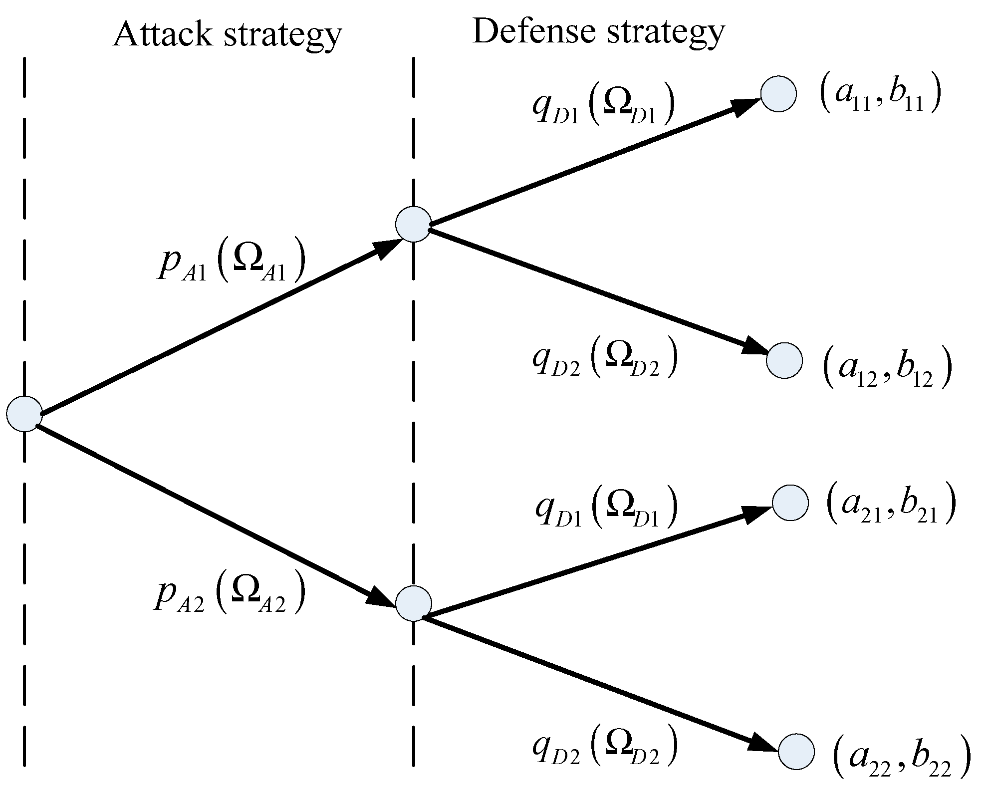
In this section, it is assumed that the attacker selects two attack strategies dynamically, and the defender selects two strategies for defense accordingly. Define $\left(a_{uv},b_{uv}\right)$ as the attack and defense payoffs when they take $\left({\Omega }_{Au},{\Omega }_{Dv}\right)$. The dynamic change rate is expressed by the solution of the replication dynamic equation.

(1)

Profits of all the players:

$$U_{Au}={\displaystyle \sum _{v=1}^m{q}_{Dv}{a}_{uv}},\overline{U_A}={\displaystyle \sum _{u=1}^n{p}_{Au}{U}_{Au}}$$

(36)

$$U_{Dv}={\displaystyle \sum _{u=1}^n{p}_{Au}{b}_{uv}},\overline{U_D}={\displaystyle \sum _{v=1}^m{q}_{Dv}{U}_{Dv}}$$

(37)

where $U_{Au}$ and $U_{Dv}$ are the expected profits for the attacker and defender. $\overline{U_A}$ and $\overline{U_D}$ are the corresponding average profits.

(2)

Replication dynamic equations for the profits:

$$\frac{d{p}_{Au}}{dt}=p_{Au}\left(U_{Au}-\overline{U_A}\right)$$

(38)

$$\frac{d{q}_{Dv}}{dt}=q_{Dv}\left(U_{Dv}-\overline{U_D}\right)$$

(39)

(3)

Stable equilibrium solution:

$$\left\{\begin{array}{l}\frac{d{p}_{Au}}{dt}=0\\ \frac{d{q}_{Dv}}{dt}=0\end{array}\right.$$

(40)

4.1.2. Evolutionary Stable Solution

In this section, a specific example with four strategies (${\Omega }_{A1}$, ${\Omega }_{D1}$), (${\Omega }_{A1}$, ${\Omega }_{D2}$), (${\Omega }_{A2}$, ${\Omega }_{D1}$), and (${\Omega }_{A2}$, ${\Omega }_{D2}$) are given for the solution of evolutionary stable equilibrium. The attacking and defending sides choose strategies with different probabilities, and generate different benefits. The game tree is shown in Figure 1.

The process of solution for the defenders and attackers can be described as follows:

(1)

Expected and average profit of a defender:

$$U_{D1}=p_{A1}{b}_{11}+p_{A2}{b}_{21}$$

(41)

$$U_{D2}=p_{A1}{b}_{12}+p_{A2}{b}_{22}$$

(42)

$${\overline{U}}_D=q_{D1}{U}_{D1}+q_{D2}{U}_{D2}$$

(43)

where $U_{D1}$ and $U_{D2}$ represent the expected profits in defense strategies 1 and 2, respectively; ${\overline{U}}_D$ represents the average profit of the defender. The replication dynamic equation of the defender over time can be represented by (44).

$$\left\{\begin{array}{l}\frac{d{q}_{D1}(t)}{dt}=q_{D1}(U_{D1}-{\overline{U}}_D)\\ \frac{d{q}_{D2}(t)}{dt}=q_{D2}(U_{D2}-{\overline{U}}_D)\end{array}\right.$$

(44)

(2)

Expected and average profit of an attacker:

$$U_{A1}=q_{D1}{a}_{11}+q_{D2}{a}_{21}$$

(45)

$$U_{A2}=q_{D1}{a}_{12}+q_{D2}{a}_{22}$$

(46)

$${\overline{U}}_A=p_{A1}{U}_{A1}+p_{A2}{U}_{A2}$$

(47)

where $U_{A1}$ and $U_{A2}$ are the expected profits in attack strategies 1 and 2, respectively; ${\overline{U}}_A$ represents the average profit of the attacker. The replication dynamic equation of the attacker over time can be represented by (48).

$$\left\{\begin{array}{l}\frac{d{p}_{A1}(t)}{dt}=p_{A1}(U_{A1}-{\overline{U}}_A)\\ \frac{d{p}_{A2}(t)}{dt}=p_{A2}(U_{A2}-{\overline{U}}_A)\end{array}\right.$$

(48)

(3)

Based on the proposed ADEG model, when $\left\{\begin{array}{l}\frac{d{q}_{D1}(t)}{dt}=-\frac{d{q}_{D2}(t)}{dt}\\ \frac{d{p}_{A1}(t)}{dt}=-\frac{d{p}_{A2}(t)}{dt}\end{array}\right.$ is satisfied, the solution can be obtained only through calculating $\left\{\begin{array}{l}\frac{d{q}_{D1}(t)}{dt}=0\\ \frac{d{p}_{A1}(t)}{dt}=0\end{array}\right.$. Through the equations, five sets of solutions for $p_{A1}$ and $q_{D1}$ can be obtained in

Table 1. Selection of the attack and defense strategies for solutions.

RDE Solutions	Defense Strategy	With Probability	Attack Strategy	With Probability
$p_{A1}=0$, $q_{D1}=0$	${\Omega }_{D1}$	0	${\Omega }_{A1}$	0
$p_{A1}=0$, $q_{D1}=1$	${\Omega }_{D2}$	1	${\Omega }_{A1}$	0
$p_{A1}=1$, $q_{D1}=0$	${\Omega }_{D1}$	0	${\Omega }_{A2}$	1
$p_{A1}=1$, $q_{D1}=1$	${\Omega }_{D2}$	1	${\Omega }_{A2}$	1
$p_{A1}=\frac{b_{22}-b_{21}}{b_{11}-b_{21}-b_{12}+b_{22}}$, $q_{D1}=\frac{a_{22}-a_{21}}{a_{11}-a_{21}-a_{12}+a_{22}}$	${\Omega }_{D1}$, ${\Omega }_{D2}$	$\begin{array}{l}(\frac{a_{22}-a_{21}}{a_{11}-a_{21}-a_{12}+a_{22}},\\ 1-\frac{a_{22}-a_{21}}{a_{11}-a_{21}-a_{12}+a_{22}})\end{array}$	${\Omega }_{A1}$, ${\Omega }_{A2}$	$\begin{array}{l}(\frac{b_{22}-b_{21}}{b_{11}-b_{21}-b_{12}+b_{22}},\\ 1-\frac{b_{22}-b_{21}}{b_{11}-b_{21}-b_{12}+b_{22}})\end{array}$

.

4.2. ADEG-Based Optimal Defense Strategy Selection

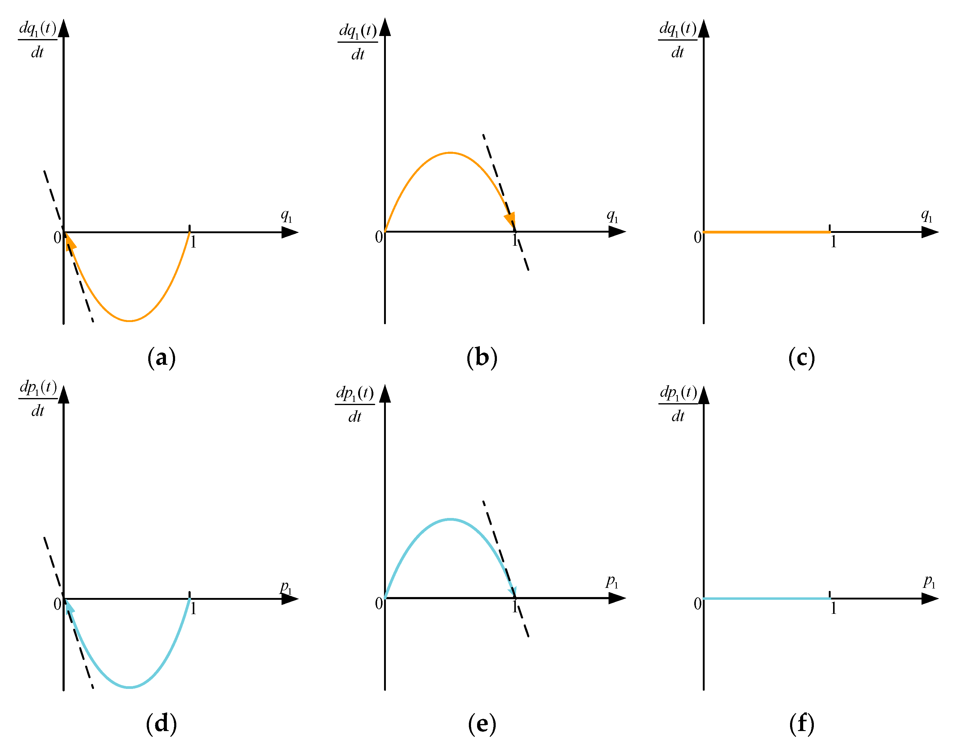
In addition to the defense strategy that the defender can choose according to the attack probability, it can also influence the attack probability selection and send messages to the attacker. In this section, the dynamic relationship between the two players is discussed through the evolutionary stable equilibrium solutions. The replication dynamic model with three situations is shown in Figure 2.

(1)

For the defender, when $p_{A1}=\frac{b_{22}-b_{21}}{b_{11}-b_{21}-b_{12}+b_{22}}$, with any probability selection of defense strategy $q_{D1}$, there is $\frac{d{q}_{D1}(t)}{dt}=0$. However, once the value of $p_{A1}$ shifts, $\frac{d{q}_{D1}(t)}{dt}$ will change dramatically, indicating that the state represented by the graph is not stable; once $p_{A1}\ne \frac{b_{22}-b_{21}}{b_{11}-b_{21}-b_{12}+b_{22}}$, $q_{D1}=0$ and $q_{D1}=1$ are two stable states. According to these, when $p_{A1}>\frac{b_{22}-b_{21}}{b_{11}-b_{21}-b_{12}+b_{22}}$, $q_{D1}=0$ is the evolution stable strategy; when $p_{A1}<\frac{b_{22}-b_{21}}{b_{11}-b_{21}-b_{12}+b_{22}}$, $q_{D1}=1$ is the strategy.

(2)

For the attacker, when $q_{D1}>\frac{a_{22}-a_{21}}{a_{11}-a_{21}-a_{12}+a_{22}}$, $p_{A1}=1$ is the strategy; when $q_{D1}<\frac{a_{22}-a_{21}}{a_{11}-a_{21}-a_{12}+a_{22}}$, $p_{A1}=0$ is the strategy; when $q_{D1}=\frac{a_{22}-a_{21}}{a_{11}-a_{21}-a_{12}+a_{22}}$, for any $p_{A1}$, there is $\frac{d{p}_{A1}(t)}{dt}=0$. However, once the value of $q_{D1}$ is shifted, $\frac{d{p}_{A1}(t)}{dt}$ will undergo significant changes, leading to an unstable state.

Define $p_A$, $q_D$ as the selection probability of attack strategies and defense strategies. After the update of the proposed hybrid game method above, the final optimal objective function of game model can be obtained as follows:

$$\max p_A\left[U_A^{*}\left({\beta }^{*},{\eta }^{*}\right)\right]\ge \max p_A\left[U_A^{*}\left(\beta ,{\eta }^{*}\right)\right]$$

(49)

$$\min q_D\left[U_D^{*}\left({\eta }^{*},{\eta }_{-}^{*},{\beta }^{*}\right)\right]\le \min q_D\left[U_D^{*}\left(\eta ,{\eta }_{-}^{*},{\beta }^{*}\right)\right]$$

(50)

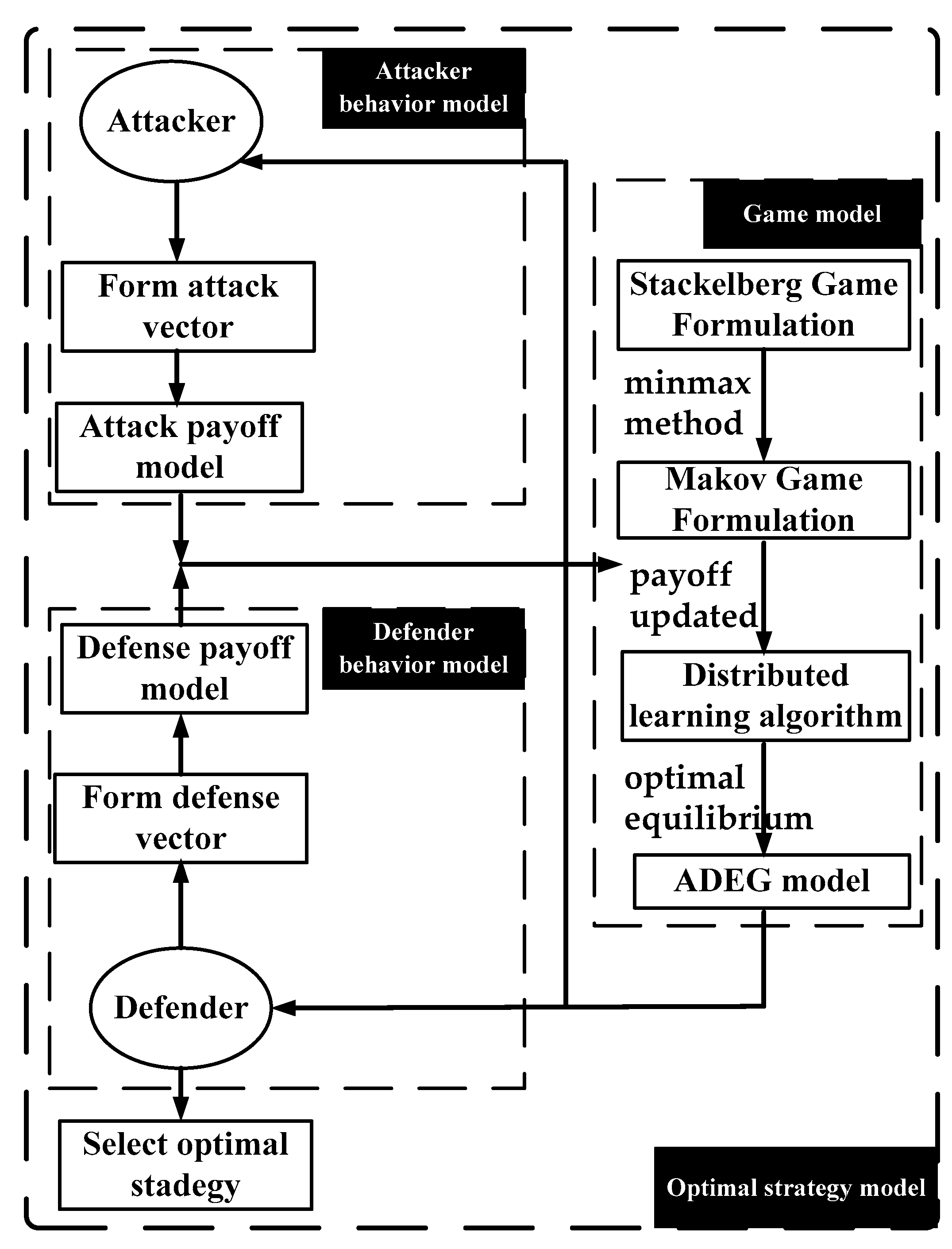
The attack–defense strategies are developed based on simulated probabilities, providing a new defense strategy selection probability in advance to cope with possible attack situations. The simplified process of obtaining the optimal defense strategy is shown in Algorithm 1.

Algorithm 1. Process of obtaining the optimal defense strategy

Phase 1-:

(1) Define the state space of power grid $S$.

(2) Define attacker’s and defender’s strategy space ${\Omega }_A$, ${\Omega }_D$.

(3) Derive state transition matrix $T\left(s,{\Omega }_A,{\Omega }_D,s^{\prime }\right)$.

(4) Find the Stackelberg equilibrium solution (${\beta }^{*},{\eta }^{*}$).

(5) Obtain the expected rewards from the attacker and defender $R_A\left(s,{\Omega }_A,{\Omega }_D\right)$, $R_D\left(s,{\Omega }_A,{\Omega }_D\right)$ according to (${\beta }^{*},{\eta }^{*}$).

Phase 2-

(1) Set initial    $Q_A\left(s,{\Omega }_A,{\Omega }_D\right)$, $Q_D\left(s,{\Omega }_A,{\Omega }_D\right)$, $V_A\left(s^{\prime }\right)$, $V_D\left(s^{\prime }\right)$

(2) Initialize $q^{\left(\omega \right)}\left(0\right)$.

while Not Converged do

Collect the payoff $r_{\omega }\left(t\right)$

Update the strategy $q^{\left(\omega \right)}\left(t+1\right)=q^{\left(\omega \right)}\left(t\right)+\epsilon r_{\omega }\left(t\right)\left(e^{\left(\omega \right)}\left(t\right)-q^{\left(\omega \right)}\left(t\right)\right)$

Check Convergence

if Converged then

break

end if

end while

(3) Return the strategy vector $q^{\left(\omega \right)}\left(t\right)$.

(4) Update $Q_A\left(s,{\Omega }_A,{\Omega }_D\right)$, $Q_D\left(s,{\Omega }_A,{\Omega }_D\right)$ according to (31), (33).

(5) Update $V_A\left(s^{\prime }\right)$, $V_D\left(s^{\prime }\right)$ according to (32), (34).

(6) Define the ADEG model.

(7) Calculate the replication dynamic equation of both of the players.

(8) Derive the optimal Stackelberg equilibrium solution according to (49), (50).

(9) Derive the final optimal strategy of the defenders through solving the equilibrium solution.

The simplified process of obtaining the optimal network defense strategy based on the hybrid game algorithm is shown in Figure 3.

5. Discussion

In this section, a simulation case is constructed to demonstrate the electricity markets attack case in an SG with MGs connected. We will verify the proposed network attack and defense game model and discuss the optimal operation. In this section, we introduced simulations using IEEE 14 bus systems and IEEE 118 bus systems.

5.1. Optimal Attack–Defense Strategies Game Model

According to the above model, system dynamics are used to verify the effect of the ADEG model. In this paper, the evolutionary stable solution is in four situations of $p_A=0, q_D=0$; $p_A=0, q_D=1$; $p_A=1, q_D=0$; and $p_A=1, q_D=1$. The two attack–defense strategies selection with different initial probabilities are listed in

Table 2. Attack strategies selection.

Initial Attack Strategies	Attacked Line	Power Flow (MW)		Attack Level (%)	Initial Probability
		Without Attack	With Attack
${\Omega }_{A1}$	2–3	54.7	27.35	50	$p_A=1$
${\Omega }_{A2}$	2–3, 4–5	54.7	49.3	10	$p_A=0$
${\Omega }_{A1}$, ${\Omega }_{A2}$	2–3, 4–5	54.7	43.9	20	$p_A=0.4$
${\Omega }_{A1}$, ${\Omega }_{A2}$	2–3	54.7	16.41	80	$p_A=0.6$

and

Table 3. Defense strategies selection.

Initial Defense Strategies	Detection Mode Selection		Initial Probability
	MGs in Grid-Connected Mode	Load Shedding
${\Omega }_{D1}$	with	without	$q_D=1$
${\Omega }_{D2}$	without	with	$q_D=0$
${\Omega }_{D1}$, ${\Omega }_{D2}$	with	with	$q_D=0.5$
${\Omega }_{D1}$, ${\Omega }_{D2}$	with	with	$q_D=0.6$

as below.

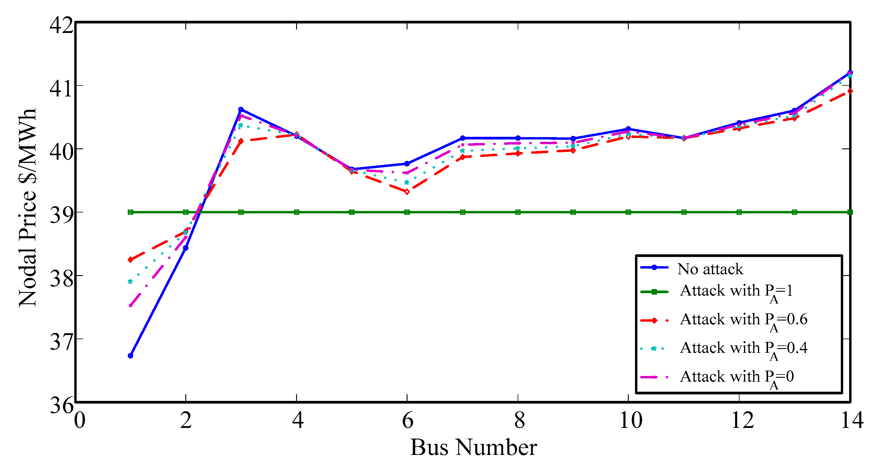
In the real-time market, prices will change after modifying the estimated line flow. The system power will be reduced below the thermal limit of the transmission line, and congested lines will be alleviated. The impact of different attack probabilities on LMP is shown in Figure 4. The proposed method will be validated using the MATPOWER 4.0 software package for age verification [29].

For further comparison, 100,000 experiments are generated in both transmission lines 2–3 and 4–5 of the IEEE-14 bus system. The ratio of attacks on two routes is 1:1. The detection performances of the four attack strategies are discussed and compared in

Table 4. Final detection result with ratio of 1:1.

Initial Attack Strategies	Detection Delay	Detection Rate
${\Omega }_{A1}$	28	85.03%
${\Omega }_{A2}$	12	90.98%
${\Omega }_{A1}$, ${\Omega }_{A2}$	9	92.01%
${\Omega }_{A1}$, ${\Omega }_{A2}$	10	95.35%

.

Based on the proposed game methods, the optimal payoff value of the two players under different game methods can be calculated and shown as follows.

5.1.1. Players with Complete Information

a.

IEEE 14-bus system

The proposed method was tested on an improved IEEE 14 bus testing system, where some of the generators were replaced by MGs with distributed and renewable generator units as well as storage units. The power value and demand are maintained under the same basic conditions as the IEEE standard 14 bus structure [30]. The system consists of one utility grid generator, four MGs, and eleven loads. MGs are located on buses 2, 3, 6, and 8, with 11 loads located on buses 2, 3, 4, 5, 6, 9, 10, 11, 12, 13, and 14. The game solution when the players obtain complete information is shown in

Table 5. Optimal attack–defense payoff value in 14-bus.

	Initial Probabilities		$\mathbf{Attack}\mathbf{Payoff}\left(\mathit{\$}\right)$		$\mathbf{Defense}\mathbf{Payoff}\left(\mathit{\$}\right)$
			$\mathbf{P}\mathbf{r}\mathbf{o}\mathbf{f}\mathbf{i}{\mathbf{t}}_{\mathbf{a}\mathbf{t}\mathbf{t}}$	$\mathbf{E}{\mathbf{L}}_{\mathbf{a}\mathbf{t}\mathbf{t}}$	${\mathit{C}}_{\mathit{D}} + {\mathit{C}}_{\mathit{G}}$	${\mathit{C}}_{\mathit{M}}$
Stackelberg method	$p_A=0$	$q_D=0$	29.38	6.35	27.32 + 0.85	5.06
	$p_A=0$	$q_D=1$	59.82	7.31	37.01 + 20.21	12.10
	$p_A=1$	$q_D=0$	67.33	13.06	32.09 + 10.50	14.88
	$p_A=1$	$q_D=1$	36.48	12.45	48.53 + 1.21	9.35
Markov Algorithm	$p_A=0$	$q_D=0$	34.41	8.25	28.44 + 0.91	5.73
	$p_A=0$	$q_D=1$	63.12	8.81	39.33 + 20.45	13.00
	$p_A=1$	$q_D=0$	37.52	12.50	49.44 + 1.81	10.01
	$p_A=1$	$q_D=1$	69.41	13.86	33.09 + 11.23	14.90
Proposed algorithm	$p_A=0$	$q_D=0$	33.31	7.05	27.00 + 0.71	5.01
	$p_A=0$	$q_D=1$	62.05	7.02	36.52 + 19.11	11.99
	$p_A=1$	$q_D=0$	36.88	10.50	46.55 + 1.05	9.12
	$p_A=1$	$q_D=1$	68.22	11.12	30.09 + 9.15	12.76

.

From Table 5, it can be concluded that:

(1)

When the attacker chooses ${\Omega }_{A1}$, the defender will choose ${\Omega }_{D1}$ to defend as the cost of $C_D$ in ${\Omega }_{D2}$ is high;

(2)

When the attacker chooses ${\Omega }_{A2}$, the defender will choose ${\Omega }_{D2}$ to defend as the cost $C_G$, $C_M$ in ${\Omega }_{D1}$ is high;

(3)

To achieve the best defense effect, the defender will choose ${\Omega }_{D1}$ when the attacker selects ${\Omega }_{A1}$, and the defender will choose ${\Omega }_{D2}$ when the attacker selects ${\Omega }_{A2}$;

(4)

When the players choose the Markov game algorithm, the profit values both increase, but the costs for both the players are also increased;

(5)

When the distributed learning algorithm is employed, the costs for two players are decreased obviously. The optimal payoff values are obtained.

Table 6. MG outputs (MW) under different initial probabilities in 14-bus.

	Pg2	Pg3	Pg6	Pg8
no attack	28.01	28.92	0.04	11.93
$p_A=0$, $q_D=0$	28	33.97	0.01	7.16
$p_A=0$, $q_D=1$	28	25.32	0.01	15.93
$p_A=1$, $q_D=0$	28	40.01	0.01	1.72
$p_A=1$, $q_D=1$	28	30	0	11.94

displays the different power generation outputs of MGs under different initial probabilities in the IEEE-14 system. Pg2~8 represent the generators of MG2~MG8:

(1)

When the defender chooses ${\Omega }_{D1}$, the power generation costs of MG2 and MG3 are low, thus the power generation is close to full output. The power generation of MG8 is lower, and MG6 keeps maintaining an isolated mode as the power generation cost is high.

(2)

When the attacker chooses ${\Omega }_{D2}$, the outputs of MG2 and MG6 remain at the same level of value. MG2 needs to purchase electricity to meet sudden changes in load demand, and MG8′s output decreases to prevent a sharp increase in the cost of the entire power system. It is obvious that when MG3 cannot purchase electricity, the output of MG8 increases sharply.

b.

IEEE 118-bus system

The IEEE 118-bus system includes 19 generators, 177 transmission lines, 9 transformers, and 91 loads [31]. The generator G1 is the reference bus, and G2–G19 that connected to buses 10, 12, 25, 26, 31, 46, 49, 54, 59, 61, 65, 66, 69, 80, 87, 89, 100, 103, and 111 are replaced by MGs. The game solution when the players obtain complete information is shown in

Table 7. Optimal attack–defense payoff value in 118-bus.

	Initial Probabilities		Attack Payoff $\left(\$\right)$		Defense Payoff $\left(\$\right)$
			${\mathbf{Profit}}_{\mathbf{a}\mathbf{t}\mathbf{t}}$	${\mathbf{EL}}_{\mathbf{a}\mathbf{t}\mathbf{t}}$	${\mathit{C}}_{\mathit{D}}+{\mathit{C}}_{\mathit{G}}$	${\mathit{C}}_{\mathit{M}}$
Stackelberg method	$p_A=0$	$q_D=0$	217.42	40.35	200.93 + 8.62	37.21
	$p_A=0$	$q_D=1$	415.31	46.52	215.66 + 140.37	76.06
	$p_A=1$	$q_D=0$	288.88	79.31	274.59 + 9.33	40.15
	$p_A=1$	$q_D=1$	428.51	80.92	212.11 + 70.38	80.75
Markov Algorithm	$p_A=0$	$q_D=0$	235.78	42.62	202.11 + 9.31	38.40
	$p_A=0$	$q_D=1$	438.42	48.11	227.72 + 142.15	78.11
	$p_A=1$	$q_D=0$	310.53	80.56	280.30 + 10.15	42.53
	$p_A=1$	$q_D=1$	451.66	83.33	223.11 + 70.56	81.15
Proposed algorithm	$p_A=0$	$q_D=0$	230.69	30.00	189.12 + 7.78	46.35
	$p_A=0$	$q_D=1$	421.83	32.45	205.38 + 130.96	78.12
	$p_A=1$	$q_D=0$	300.96	68.91	260.45 + 8.89	48.49
	$p_A=1$	$q_D=1$	440.72	70.83	208.30 + 68.55	89.70

.

From Table 7, it can be concluded that:

(1)

Compared with the IEEE-14 system, the effect of the distributed learning algorithm in the IEEE-118 system is better, but the computational complexity increases, thus the value of $C_M$ is higher;

(2)

The IEEE-118 system is more complex with many generators and loads, and $C_D$ and $C_G$ are higher, but the profit of the attacker is lower, and the defense effect is better;

(3)

The difference between defense cost is smaller in the IEEE-118 system, and the proposed game method is numerically better than other game methods at the equilibrium point, indicating that the method proposed in this paper is suitable for complex large systems.

5.1.2. Players with Partial Information

The optimal payoff value for the two players in partial information with system topology is shown in

Table 8. Optimal attack–defense payoff value.

	Initial Probabilities		$\mathbf{Attack}\mathbf{Payoff}\left(\mathit{\$}\right)$		$\mathbf{Defense}\mathbf{Payoff}\left(\mathit{\$}\right)$
			$\mathbf{P}\mathbf{r}\mathbf{o}\mathbf{f}\mathbf{i}{\mathbf{t}}_{\mathbf{a}\mathbf{t}\mathbf{t}}$	$\mathbf{E}{\mathbf{L}}_{\mathbf{a}\mathbf{t}\mathbf{t}}$	${\mathit{C}}_{\mathit{D}} + {\mathit{C}}_{\mathit{G}}$	${\mathit{C}}_{\mathit{M}}$
IEEE-14 system	$p_A=0.4$	$q_D=0.5$	28.12	5.11	24.00 + 6.15	7.12
	$p_A=0.4$	$q_D=0.6$	36.33	4.89	28.30 + 23.52	13.00
	$p_A=0.6$	$q_D=0.5$	29.00	8.32	44.12 + 8.35	11.54
	$p_A=0.6$	$q_D=0.6$	40.15	9.06	29.11 + 15.30	14.98
IEEE-118 system	$p_A=0.4$	$q_D=0.5$	189.45	20.83	170.35 + 14.56	50.34
	$p_A=0.4$	$q_D=0.6$	405.61	21.42	200.11 + 160.50	84.12
	$p_A=0.6$	$q_D=0.5$	289.33	60.35	230.25 + 16.35	50.66
	$p_A=0.6$	$q_D=0.6$	410.54	68.44	198.45 + 82.31	94.30

. The game solution is obtained in both the IEEE-14 system and the IEEE-118 system.

Table 9. MG outputs (MW) under different initial probabilities in 118-bus.

	Pg2	Pg3	Pg6	Pg8
no attack	28.01	28.92	0.04	11.93
$p_A=0.4,q_D=0.5$	28	29.99	0.01	12.58
$p_A=0.4,q_D=0.6$	28.01	29.99	0.04	13.15
$p_A=0.6,q_D=0.5$	28	40.01	0.01	11.68
$p_A=0.6,q_D=0.6$	28.01	40.01	0.04	14.10

shows the generation outputs of MGs considering different game methods.

From Table 8 and Table 9, it can be concluded that:

(1)

When the players have partial information, payoff on both sides is reduced, as the attack is not established completely and the defense is not using the optimal strategy;

(2)

In this situation, the cost of $C_G$ is higher than $C_D$, and defenders choose to readjust the generator output instead of shedding loads;

(3)

When the mixed strategy is chosen, the defense effect of the IEEE-118 system is better than the IEEE-14 system because the generator and load are more complex.

For maximum attack–defense benefits, the selection of the optimal defense strategy should refer to the continuous evolution of attack and defense probability. In the next subsection, the final defense strategy is established according to the ADEG model.

5.2. ADEG-Based Optimal Defense Strategy Selection

5.2.1. Effectiveness of the ADEG Model

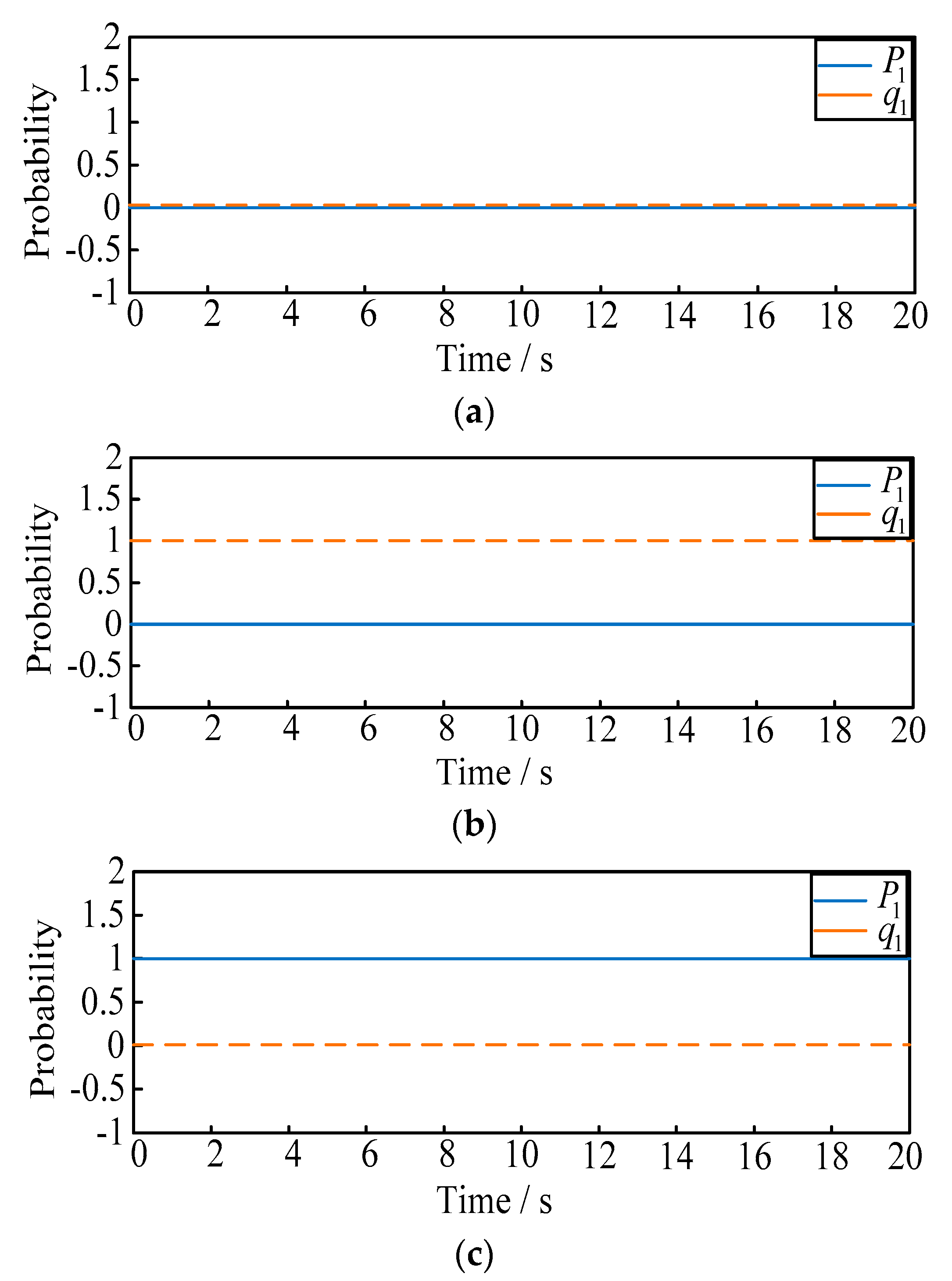
The purpose of this case is to verify the influence of the dynamic evolution of probability on the strategy, and the selection of the optimal defense strategies under different initial probabilities shown above. Based on the evolutionary stable solutions, experimental results of the evolution trend can be obtained as in Figure 5a–j.

(1)

From Figure 5a–d, when $p_A=1$ or $p_A=0$, the final selection probability of the attacker is always 1 or 0. Similarly when $q_D=1$ or $q_D=0$, the final selection probability of the defender is always 1 or 0;

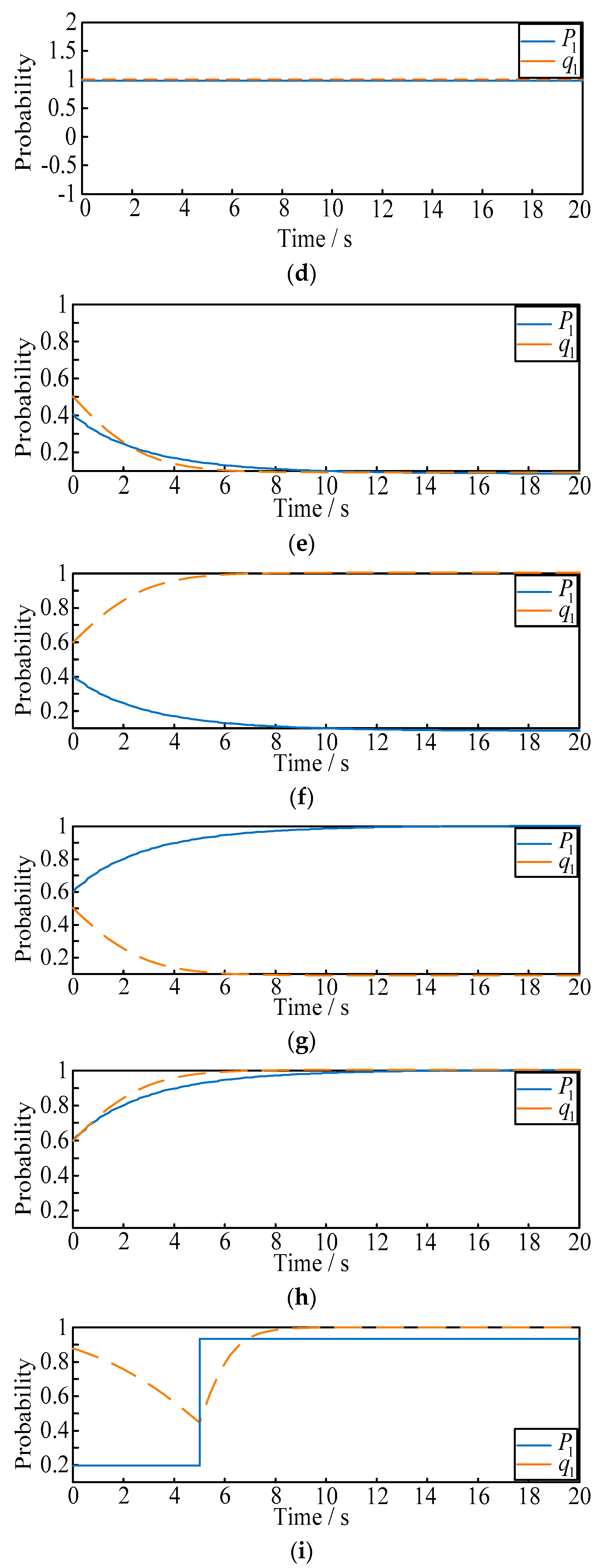
(2)

From Figure 5e–h, when the mixed probability strategies are selected, the stable solution will be $\frac{b_{22}-b_{21}}{b_{11}-b_{21}-b_{12}+b_{22}}=0.51$ and $\frac{a_{22}-a_{21}}{a_{11}-a_{21}-a_{12}+a_{22}}=0.59$. Then, when the initial attack probability is larger than 0.51, the final selection probability of the defender will eventually change to 1; when the initial attack probability is less than 0.51, the final selection probability of the defender will eventually change to 0. Similarly for the attacker, when the initial defense probability is larger than 0.59, the final selection probability of the attacker will eventually change to 1; when the initial defense probability is less than 0.59, the final selection probability of the attacker will eventually change to 0;

(3)

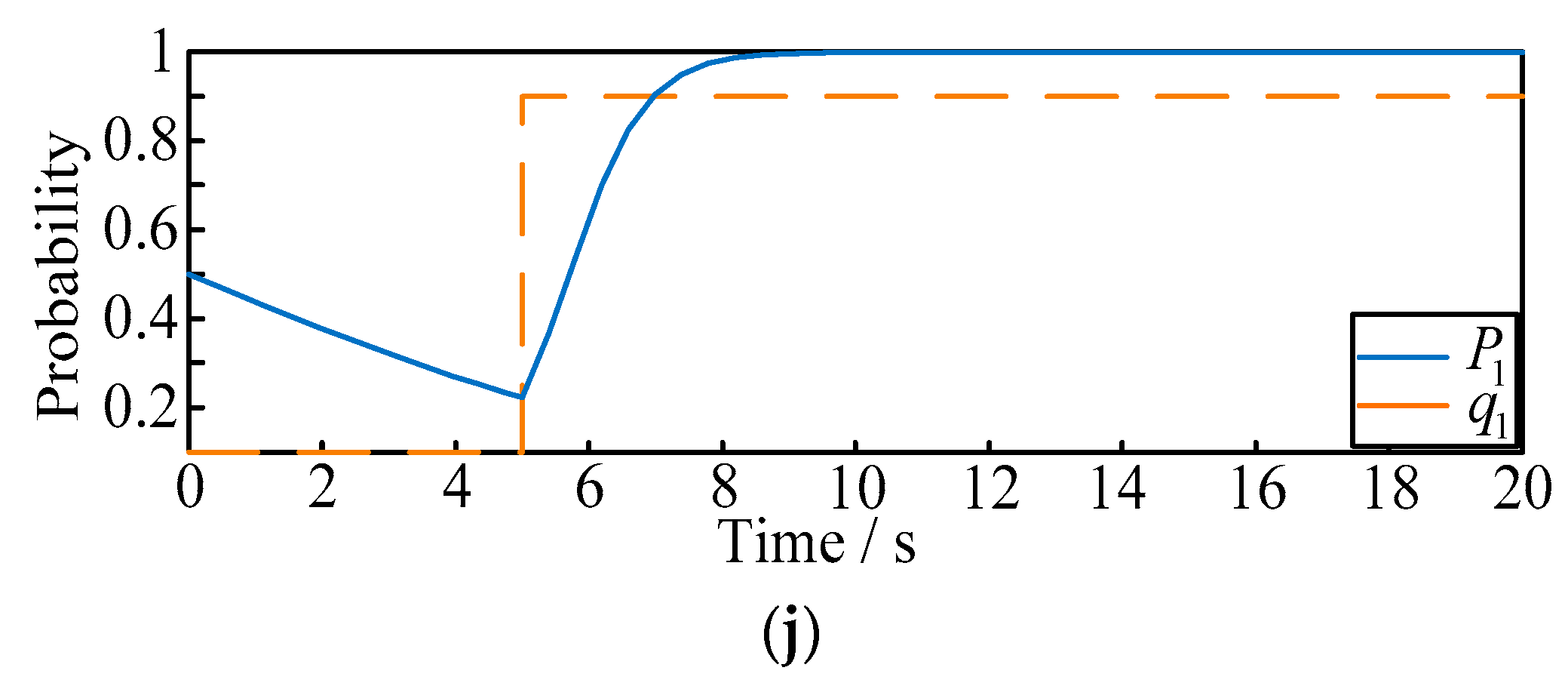
To further illustrate the dynamic effect of ADEG model, and verify the probability that the two players can be affected by each other, the following scenarios are proposed as shown in Figure 5i,j:

(a)

Situation 1: the initial probability of $p_A$ and $q_D$ are selected as fixed values of 0.2 and 0.9. When t = 5 s, we make $p_A$ suddenly rise to 0.8, and observe the variation of $q_D$;

(b)

Situation 2: the initial probability of $p_A$ and $q_D$ are selected as fixed values of 0.5 and 0. When t = 5 s, we make $q_D$ suddenly rise to 0.9, and observe the variation of $p_A$.

5.2.2. Final Defense Strategies Selection

From the cases, the conclusion can be drawn that the selection probability of attack and defense strategy will change in real time, and the two players will change the probability of the attack–defense strategy choice considering the current game situation. The purpose of the defender is to select the final optimal defense strategies according to the evolutionary stable solutions. Define ${\Omega }_{D1}=\left(q_D=0\right)$, ${\Omega }_{D2}=\left(q_D=1\right)$, then the final optimal defense strategies can be chosen as follows:

(1)

For the fixed value of the evolutionary stable solutions, the final optimal defense strategies are selected in

Table 10. Optimal defense strategies selection 1.

Initial Probabilities	Evolutionary Stable Solutions	Final Defense Strategies
$p_A=0,q_D=0$	$p_A=0,q_D=0$	${\Omega }_{D1}$
$p_A=0,q_D=1$	$p_A=0,q_D=1$	${\Omega }_{D2}$
$p_A=1,q_D=0$	$p_A=1,q_D=0$	${\Omega }_{D1}$
$p_A=1,q_D=1$	$p_A=1,q_D=1$	${\Omega }_{D2}$

;

(2)

For the mixed selection of initial probabilities, the final optimal defense strategies are selected in

Table 11. Optimal defense strategies selection 2.

Initial Probabilities	Evolutionary Stable Solutions	Final Defense Strategies
$p_A=0.4,q_D=0.5$	$p_A=0,q_D=0$	${\Omega }_{D1}$
$p_A=0.4,q_D=0.6$	$p_A=0,q_D=1$	${\Omega }_{D2}$
$p_A=0.6,q_D=0.5$	$p_A=1,q_D=0$	${\Omega }_{D1}$
$p_A=0.6,q_D=0.6$	$p_A=1,q_D=1$	${\Omega }_{D2}$

;

(3)

When the mixed selection of initial probabilities changes in real time, the final optimal defense strategies are selected in

Table 12. Optimal defense strategies selection 3.

Initial Probabilities	Probabilities Change	Final Defense Strategies
$p_A=0.4,q_D=0.5$	$p_A=0.5\to 0.9$	${\Omega }_{D1}\to {\Omega }_{D2}$
$p_A=0.4,q_D=0.6$	$p_A=0.6\to 0.2$	${\Omega }_{D2}\to {\Omega }_{D1}$
$p_A=0.6,q_D=0.5$	$p_A=0.5\to 0.9$	${\Omega }_{D1}\to {\Omega }_{D2}$
$p_A=0.6,q_D=0.6$	$p_A=0.6\to 0.2$	${\Omega }_{D2}\to {\Omega }_{D1}$

;

(4)

To illustrate the effectiveness of the ADEG model in selecting strategies, dynamic situations with a constant value of initial probabilities have been shown in

Table 13. Optimal defense strategies selection 4.

Initial Probabilities	Probabilities Change	Final Defense Strategies
$p_A=0.4$ (fixed value), $q_D=0.5$	$p_A=0.4\to 0.9$	${\Omega }_{D1}\to {\Omega }_{D2}$
$p_A=0.4$ (fixed t value), $q_D=0.6$	$p_A=0.4\to 0.1$	${\Omega }_{D1}\to {\Omega }_{D1}$
$p_A=0.6$ (fixed value), $q_D=0.5$	$p_A=0.6\to 0.1$	${\Omega }_{D2}\to {\Omega }_{D1}$
$p_A=0.6$ (fixed value), $q_D=0.6$	$p_A=0.6\to 0.9$	${\Omega }_{D2}\to {\Omega }_{D2}$

.

6. Conclusions

To analyze the dynamic game behavior of attackers and defenders in the electricity markets and choose the optimal defense strategy for the defender, this paper has carried out the following work through using hybrid game methods: firstly, the power market model with MG participation while considering FDI attack is established using the Nash equilibrium method. Influence on the impact of the optimization output for MGs energy management is discussed. Meanwhile, the behaviors of both the attackers and defenders are discussed. The payoff functions of the two players are constructed and solved via the Stackelberg equilibrium algorithm. The Markov game algorithm and distributed learning algorithm are used to update the payoff function; secondly, evolutionary game theory is used to discuss the dynamic game behavior of the two players, according to the analysis of the attack–defense probability. The optimal defense strategy is selected according to the dynamic changing probability; finally, based on the evolutionary stability strategy, the final optimal defense strategies selection algorithm is designed. The strategies are considered with different initial attack probabilities and evolutionary stable solutions. Modified IEEE standard bus systems are illustrated to certify the effectiveness of the proposed model. The simulation results have shown the game relationship between the benefits of both attack and defense sides, and the important role of the optimal output of MGs. In addition, the proposed ADEG model is proved to be effective with different initial probabilities, and the optimal defense strategy can be derived from the evolutionary model.

In the future, defense strategy selection when attacks are unpredictable will be studied.

References

- Shahid, K.; Nainar, K.; Olsen, R.L.; Iov, F.; Lyhne, M.; Morgante, G. On the Use of Common Information Model for Smart Grid Applications—A Conceptual Approach. IEEE Trans. Smart Grid 2021, 12, 5060–5072. [Google Scholar] [CrossRef]
- Habibi, M.R.; Baghaee, H.R.; Blaabjerg, F.; Dragičević, T. Secure MPC/ANN-Based False Data Injection Cyber-Attack Detection and Mitigation in DC Microgrids. IEEE Syst. J. 2022, 16, 1487–1498. [Google Scholar] [CrossRef]
- Li, B.; Lu, R.; Xiao, G.; Li, T.; Choo, K.-K.R. Detection of False Data Injection Attacks on Smart Grids: A Resilience-Enhanced Scheme. IEEE Trans. Power Syst. 2021, 37, 2679–2692. [Google Scholar] [CrossRef]
- Rodríguez, M.; Betarte, G.; Calegari, D. A Process Mining-based approach for Attacker Profiling. In Proceedings of the 2021 IEEE URUCON, Montevideo, Uruguay, 24–26 November 2021; pp. 425–429. [Google Scholar]
- Sandal, Y.S.; Pusane, A.E.; Kurt, G.K.; Benedetto, F. Reputation Based Attacker Identification Policy for Multi-Access Edge Computing in Internet of Things. IEEE Trans. Veh. Technol. 2020, 69, 15346–15356. [Google Scholar] [CrossRef]
- Rappoport, J.S. The Problem of Approach of Controlled Objects in Dynamic Game Problems with a Terminal Payoff Function. Cybern. Syst. Anal. 2020, 56, 820–834. [Google Scholar] [CrossRef]
- Zhang, B.; Dou, C.; Yue, D.; Park, J.H.; Zhang, Y.; Zhang, Z. Game and Dynamic Communication Path-Based Pricing Strategies for Microgrids under Communication Interruption. IEEE/CAA J. Autom. Sin. 2023, 10, 1032–1047. [Google Scholar] [CrossRef]
- Aydeger, A.; Manshaei, M.H.; Rahman, M.A.; Akkaya, K. Strategic Defense Against Stealthy Link Flooding Attacks: A Signaling Game Approach. IEEE Trans. Netw. Sci. Eng. 2021, 8, 751–764. [Google Scholar] [CrossRef]
- Liu, Z.; Wang, L. Defense Strategy Against Load Redistribution Attacks on Power Systems Considering Insider Threats. IEEE Trans. Smart Grid 2021, 12, 1529–1540. [Google Scholar] [CrossRef]
- Pirani, M.; Nekouei, E.; Sandberg, H.; Johansson, K.H. A Graph-Theoretic Equilibrium Analysis of Attacker-Defender Game on Consensus Dynamics under H2 Performance Metric. IEEE Trans. Netw. Sci. Eng. 2021, 8, 1991–2000. [Google Scholar] [CrossRef]
- Li, Y.; Bai, S.; Gao, Z. A Multi-Domain Anti-Jamming Strategy Using Stackelberg Game in Wireless Relay Networks. IEEE Access 2020, 8, 173609–173617. [Google Scholar] [CrossRef]
- Jakóbik, A. Stackelberg Game Modeling of Cloud Security Defending Strategy in the Case of Information Leaks and Corruption. Simul. Model. Pract. Theory 2020, 103, 102071. [Google Scholar] [CrossRef]
- Chen, Z.; Cui, G.; Zhang, L.; Yang, X.; Li, H.; Zhao, Y.; Ma, C.; Sun, T. Optimal Strategy for Cyberspace Mimic Defense Based on Game Theory. IEEE Access 2021, 9, 68376–68386. [Google Scholar] [CrossRef]
- Zhou, Y.; Cheng, G.; Zhao, Y.; Chen, Z.; Jiang, S. Toward Proactive and Efficient DDoS Mitigation in IIoT Systems: A Moving Target Defense Approach. IEEE Trans. Ind. Inform. 2022, 18, 2734–2744. [Google Scholar] [CrossRef]
- Zhang, Z.; Huang, S.; Chen, Y.; Li, B.; Mei, S. Cyber-Physical Coordinated Risk Mitigation in Smart Grids Based on Attack-Defense Game. IEEE Trans. Power Syst. 2022, 37, 530–542. [Google Scholar] [CrossRef]
- Emadi, H.; Clanin, J.; Hyder, B.; Khanna, K.; Govindarasu, M.; Bhattacharya, S. An Efficient Computational Strategy for Cyber-Physical Contingency Analysis in Smart Grids. In Proceedings of the 2021 IEEE Power & Energy Society General Meeting (PESGM), Washington, DC, USA, 26–29 July 2021; pp. 1–5. [Google Scholar]
- Shi, Y.; Rong, Z. Analysis of Q-Learning Like Algorithms Through Evolutionary Game Dynamics. IEEE Trans. Circuits Syst. II Express Briefs 2022, 69, 2463–2467. [Google Scholar] [CrossRef]
- Zhang, H.; Tan, J.; Liu, X.; Huang, S.; Hu, H.; Zhang, Y. Cybersecurity Threat Assessment Integrating Qualitative Differential and Evolutionary Games. IEEE Trans. Netw. Serv. Manag. 2022, 19, 3425–3437. [Google Scholar] [CrossRef]
- Chen, G.; Yu, Y. Convergence Analysis and Strategy Control of Evolutionary Games with Imitation Rule on Toroidal Grid. IEEE Trans. Autom. Control. 2023, 68, 8185–8192. [Google Scholar] [CrossRef]
- Zhang, B.; Dou, C.; Yue, D.; Zhang, Z.; Zhang, T. A Packet Loss-Dependent Event-Triggered Cyber-Physical Cooperative Control Strategy for Islanded Microgrid. IEEE Trans. Cybern. 2021, 51, 267–282. [Google Scholar] [CrossRef] [PubMed]
- Monica, P.; Kowsalya, M.; Guerrero, J.M. Logarithmic droop-based decentralized control of parallel converters for accurate current sharing in islanded DC microgrid applications. IET Renew. Power Gener. 2021, 15, 1240–1254. [Google Scholar]
- Mohammadhassani, A.; Teymouri, A.; Mehrizi-Sani, A.; Tehrani, K. Performance Evaluation of an Inverter-Based Microgrid Under Cyberattacks. In Proceedings of the 2020 IEEE 15th International Conference of System of Systems Engineering (SoSE), Budapest, Hungary, 2–4 June 2020. [Google Scholar] [CrossRef]
- Liu, C.; Zhou, M.; Wu, J.; Long, C.; Kundur, D. Financially Motivated FDI on SCED in Real-Time Electricity Markets: Attacks and Mitigation. IEEE Trans. Smart Grid 2019, 10, 1949–1959. [Google Scholar] [CrossRef]
- Hasankhani, A.; Hakimi, S.M. Stochastic energy management of smart microgrid with intermittent renewable energy resources in electricity market. Energy 2021, 219, 119668. [Google Scholar] [CrossRef]
- Razmi, P.; Buygi, M.O.; Esmalifalak, M. A Machine Learning Approach for Collusion Detection in Electricity Markets Based on Nash Equilibrium Theory. J. Mod. Power Syst. Clean Energy 2021, 9, 170–180. [Google Scholar] [CrossRef]
- Dou, C.; Yue, D.; Li, X.; Xue, Y. Mas-based management and control strategies for integrated hybrid energy system. IEEE Trans. Ind. Inform. 2016, 12, 1332–1349. [Google Scholar] [CrossRef]
- Major, J.A. Advanced techniques for modeling terrorism risk. J. Risk Financ. 2002, 4, 15–24. [Google Scholar] [CrossRef]
- Ma, C.Y.T.; Yau, D.K.Y.; Lou, X.; Rao, N.S. Markov Game Analysis for Attack-Defense of Power Networks under Possible Misinformation. IEEE Trans. Power Syst. 2012, 28, 1676–1686. [Google Scholar] [CrossRef]
- Zimmerman, R.D.; Murillo-Sanchez, C.E.; Thomas, R.J. MATPOWER: Steady-State Operations, Planning, and Analysis Tools for Power Systems Research and Education. IEEE Trans. Power Syst. 2011, 26, 12–19. [Google Scholar] [CrossRef]
- Foo Eddy, Y.S.; Gooi, H.B.; Chen, S.X. Multi-agent system for distributed management of microgrids. IEEE Trans. Power Syst. 2015, 30, 24–34. [Google Scholar] [CrossRef]
- Hassan, M.H.; Kamel, S.; El-Dabah, M.A.; Khurshaid, T.; Domínguez-García, J.L. Optimal Reactive Power Dispatch with Time-Varying Demand and Renewable Energy Uncertainty Using Rao-3 Algorithm. IEEE Access 2021, 9, 23264–23283. [Google Scholar] [CrossRef]
Figure 1.
The proposed attack–defense game tree.
Figure 2.
The replication dynamic model curve. (a) The variation of the defender when . (b) The variation of the defender when . (c) The variation of the defender when . (d) The variation of the attacker when . (e) The variation of the attacker when . (f) The variation of the attacker when .
Figure 3.
The selection of the optimal network defense strategy.
Figure 4.
LMPs with different attack probabilities.
Figure 5.
(a–d) The evolution curve of attack and defense strategies. (a) The evolution curve with the initial probability (). (b) The evolution curve with the initial probability (). (c) The evolution curve with the initial probability (). (d) The evolution curve with the initial probability (). (e–h). The evolution curve of attack and defense strategies. (e) The evolution curve with the initial probability (). (f) The evolution curve with the initial probability (). (g) The evolution curve with the initial probability (). (h) The evolution curve with the initial probability (). (i,j). Real-time evolution curve of attack and defense strategies. (i) The evolution curve in situation 1. (j) The evolution curve in situation 2.