

Shifting Pattern Biclustering and Boolean Reasoning Symmetry


1
Department of Computer Networks and Systems, Silesian University of Technology, ul. Akademicka 16, 44-100 Gliwice, Poland
2
Łukasiewicz Research Network—Institute of Innovative Technologies EMAG, ul. Leopolda 31, 40-189 Katowice, Poland
3
School of Engineering, Pablo de Olavide University, 41013 Seville, Spain
*
Author to whom correspondence should be addressed.
Symmetry 2023, 15(11), 1977; https://doi.org/10.3390/sym15111977
Submission received: 25 August 2023
/
Revised: 12 October 2023
/
Accepted: 23 October 2023
/
Published: 26 October 2023
(This article belongs to the Special Issue Machine Learning and Data Analysis II)
Abstract
:There are several goals of the two-dimensional data analysis: one may be interested in searching for groups of similar objects (clustering), another one may be focused on searching for some dependencies between a specified one and other variables (classification, regression, associate rules induction), and finally, some may be interested in serching for well-defined patterns in the data called biclusters. It was already proved that there exists a mathematically proven symmetry between some patterns in the matrix and implicants of data-defined Boolean function. This paper provides the new look for a specific pattern search—the pattern named the -shifting pattern. The shifting pattern is interesting, as it accounts for constant fluctuations in data, i.e., it captures situations in which all the values in the pattern move up or down for one dimension, maintaining the range amplitude for all the dimensions. Such a behavior is very common in real data, e.g., in the analysis of gene expression data. In such a domain, a subset of genes might go up or down for a subset of patients or experimental conditions, identifying functionally coherent categories. A -shifting pattern meets the necessity of shifting pattern induction together with the bias of the real values acquisition where the original shifts may be disturbed with some outer conditions. Experiments with a real dataset show the potential of our approach at finding biclusters with -shifting patterns, providing excellent performance. It was possible to find the pattern in the input data with . The experiments also revealed that -shifting patterns are quite difficult to be found by some well-known methods of biclustering, as these are not designed to focus on shifting patterns—results comparable due to had much more variability (in terms of ) than patterns found with Boolean reasoning.
1. Introduction
Biclustering is a two-dimensional clustering technique considered first by Morgan and Sonquist [1], and subsequently by Hartigan [2] and by Mirkin [3], although it was popularized by Cheng and Church [4] in the context of gene expression data analysis. It has an interesting property that is not fulfilled by clustering techniques: a value from the matrix (dataset) could belong to zero, one or more biclusters. In other words, the join of all the biclusters might not be the original dataset, and the intersection of two biclusters might not be empty. In many contexts, biclustering results are more appropriate, as they focus on more specific patterns (subsets of rows and columns, simultaneously) than those provided by clustering (row or column segmentation, independently). Apart from the fact that the computational complexity is higher than that of clustering (exponential), becoming a NP-hard problem [5], biclustering has captured the attention of the scientific community because it is able to search for more specific patterns in data (medical [6], environmental [7], biological [8], text mining [9,10], and many others [11]), discarding naturally what is not relevant for the goals [12].
In general, the extraction of biclusters from data is organized in two processes: the search for biclusters in the high-dimensional search space (exploration), and the selection of good biclusters by means of a quality function (exploitation). The goal is to find a sub-matrix that shows a behavioral pattern for rows and columns simultaneously. Patterns can adopt different structures, depending on the definition of behavior associated to the values within the bicluster [13]. However, there are two types of patterns that show special interest in nature: shifting and scaling patterns [14]. Most of the approaches for shifting pattern induction are based on a measure named Mean Square Residue () [4] and its variants [15,16,17,18], or on graph theory [19,20,21].
During the last two decades, different heuristics have been developed that provide sets of biclusters: based on graphs [5,22,23], uncovering structures by eigenvectors [24], based on evolutionary computation [25], ensemble methods [26], or scatter search [27], which are evaluated with some measure of quality [28,29,30,31]. However, they mainly focused on the type of bicluster (as defined in [13]) rather than on the type of pattern [14].
The process of searching for biclusters in data can be addressed with different paradigms. In the formal concept analysis realm [32], the extraction of the concept lattice is equivalent to finding inclusion-maximal biclusters in binary data. Similarly, the bicluster of ones in binary data, which refers to market basket analysis [33] (a special case of affinity analysis [34]), may be easily interpreted as frequent item sets. Also from the graph theory point of view, it may be interesting to detect such patterns in different graph describing matrices [35].
This work presents a new approach for pattern extraction based on a symmetry between searching for patterns in the data and Boolean reasoning [36]. Its novelty consists of two aspects: it extends both the general biclustering approach started in [37] for binary and discrete data and the later extended for continuous data, and it also provides the definition of a new type of bicluster named the -shifting pattern. The rationale behind the approach is based on the possibility of representing data differences as Boolean formulas, whose implicants (and prime implicants) encode the biclusters (such correspondence between biclusters and implicants is mathematically proven). In fact, shifting pattern induction is possible since Boolean reasoning provides the skills for finding all inclusion-maximal -shifting patterns.
The paper is organized as follows: firstly, a short introduction of the most important concepts and of several types of patterns, which might be the goal of the search; next, a brief presentation of the Boolean reasoning paradigm application to biclustering of continuous data; later, Section 4 provides the necessary definitions and theorems for finding constant and -shifting patterns; the experimental analysis of the approach on real data is provided next together with the description of the obtained results; finally, discussion and further work in the area of Boolean reasoning-based pattern induction are also presented.
2. Theoretical Background
2.1. Biclustering
Clustering is a technique of unsupervised data analysis, where the goal is to find similar groups of multidimensional objects, which are described by heterogeneous attributes. Considering the set of objects O, the result of clustering is the partition—in terms of mathematical definition—of O into a family of disjoint, nonempty subsets of O, whose union of all of them is O.
On the other hand, biclustering tries to find patterns in a two-dimensional matrix of scalars (homogeneous values from the same domain), whose patterns satisfy a well-defined criterion [38]. Therefore, biclustering results are not necessarily disjoint, and the union might not cover the original matrix.
Definition 1
(Matrix). A matrix (referring to the dataset) is defined as a tuple where are two finite sets referred to as the set of rows and the set of columns, respectively.
A matrix , is therefore defined by , ⋯, , , where each position contains a value from the same domain (a real value, in general):
Commonly, the indexes of and are natural numbers. However, in this paper, those natural indexes will be interpreted as nominal labels, so as the inclusion relation of row/column indexes is implicit. In other words, we do not keep the order of rows/columns but just use natural numbers as a row/column symbolic identifier.
Definition 2
(Bicluster). A bicluster is a 2-tuple =, =, where , and , and it satisfies .
Hereafter, for simplicity, the bicluster will be represented as a matrix of values or enumerating the subset of rows and columns as , and generically, with the expression . As and are subsets of and , respectively, empty biclusters will be identified when any of those subsets are empty.
Considering some criterion , it is possible to define the inclusion-maximal bicluster as follows:
Definition 3
(Inclusion-Maximal Bicluster). Let =, be a bicluster of the matrix whose elements satisfy the criterion . The bicluster is inclusion-maximal if there is neither nor such that any extended biclusters or still satisfy the criterion . In other words, subsets and are maximal subsets (in the sense of inclusion) of sets and , respectively.
The above definition is very important in the following because of the possibilities of the Boolean reasoning approach to find biclusters satisfying the stated criterion.
2.2. Bicluster Typology
The previous subsection has provided general definitions for biclustering, since they only address structure but not properties. Henceforth, depending on the type of input data domain, as well as the expectations of the data owner, it is possible to qualify the properties it must fulfill. For instance, for discrete data, the intuitive requirement is to contain constant values; and for binary matrices, the interest resides on biclusters of only ones. However, continuous-valued matrices are more complex and offer a number of patterns, among them:
- Tolerance bicluster
- Center-based bicluster
- Perfect bicluster, satisfying one of the following (the symbol represents addition or multiplication):
- –
- All the values are equal (equivalent to considering continuous data as discrete);
- –
- where is a typical value within the bicluster and is the adjustment for row ;
- –
- where is a typical value within the bicluster and is the adjustment for column ;
- –
- , which is a combination of the above two.
A special case of a perfect bicluster is called a shifting pattern (). Given its importance, an illustrative example of the shifting pattern is introduced next.
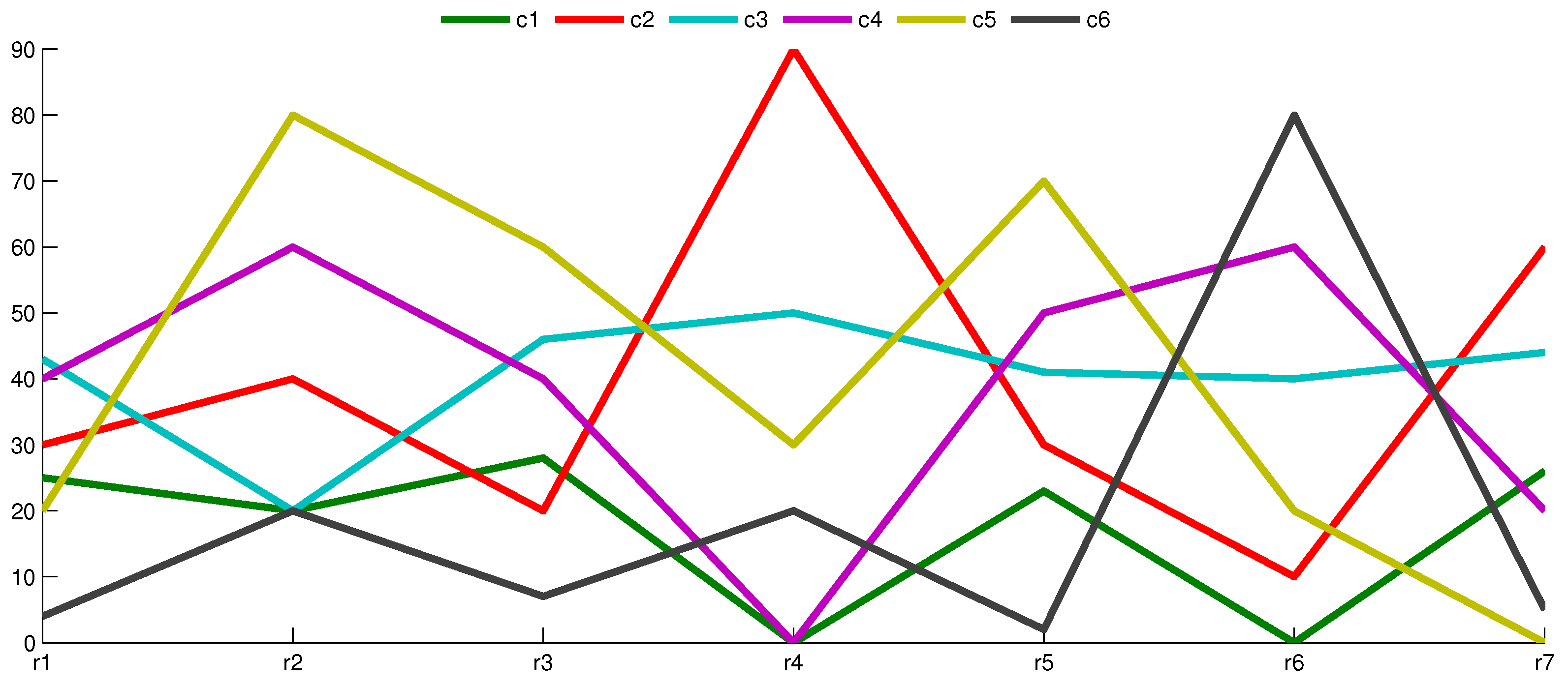
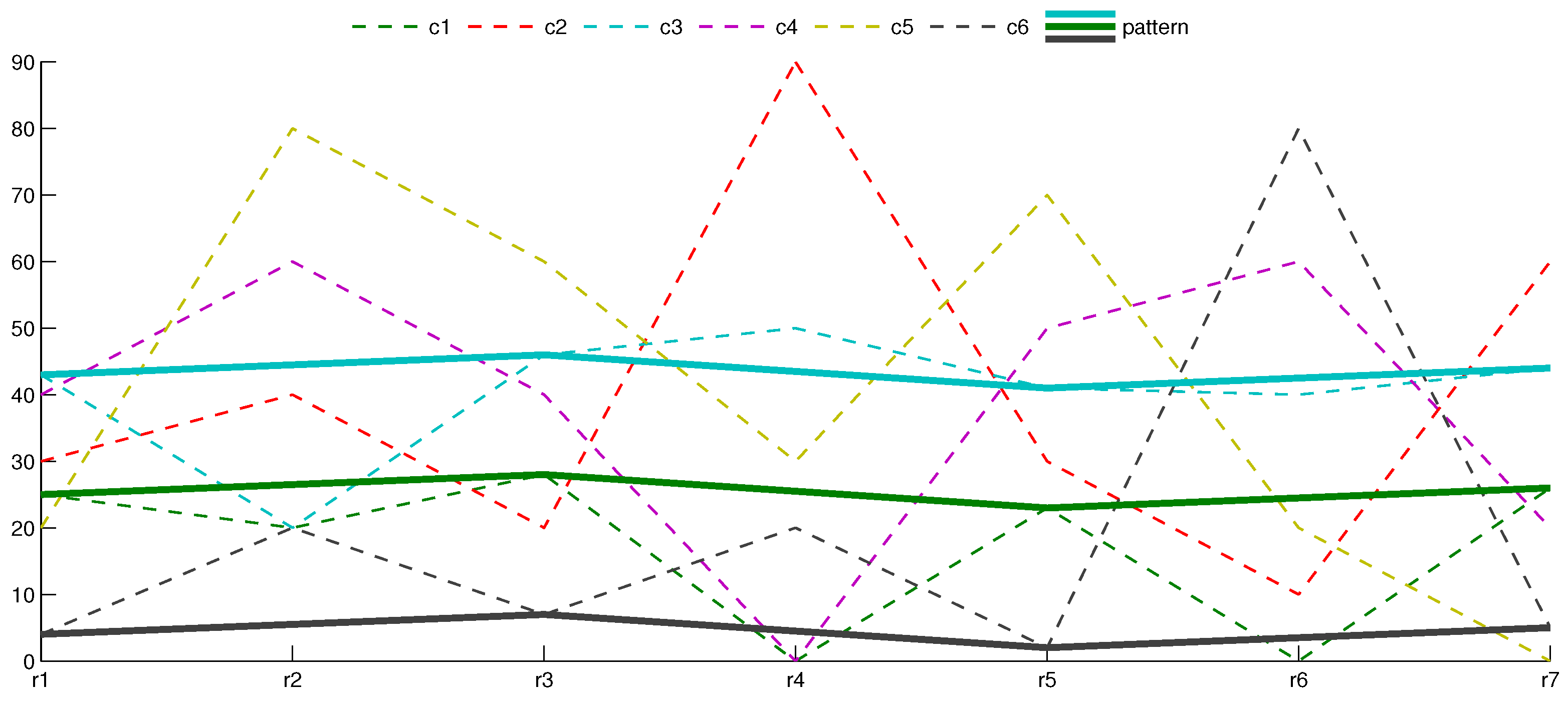
Let a matrix have seven rows (X axis values) and six columns (color lines), as depicted in Figure 1. Each column c of the data is presented as the line going through rows indicated in the X axis.
It is not so intuitive to discover hidden shifting patterns in Figure 1. However, at least one such pattern exists—, , —and it is highlighted in Figure 2 with solid lines over the dashed ones.
Due to the nature of data, which very frequently includes noise, perfect biclusters are not common in real-world data. Only an infinitesimal variation of a matrix value would cause the row and column where it is placed to not be both selected for a bicluster. Thus, a -shifting pattern emerges as an effective alternative to detect shifting patterns with small noise presence (a definition will be provided in Section 4.2).
3. Boolean Reasoning and Biclustering
The first applications of the Boolean reasoning paradigm in the domain of biclustering were published by Michalak and Ślȩzak [37], in which mathematical foundations were provided for discrete value matrices [39]. The intuitive generalization of such an approach for continuous data was also presented. However, both previous approaches did not deal with shifting patterns, as those addressed the search for global patterns, which fluctuate within a range (a global bandwidth). This work, instead, introduces a Boolean reasoning-based approach to search for -shifting patterns, which are much more interesting due to their usefulness in many domains (e.g., gene expression data analysis [14]).
Biclustering based on Boolean reasoning moves the search for biclusters to the aim of finding some Boolean formula implicants or prime implicants. The formal definition of the formula depends on the input data domain and the objective of the analysis (requirements of the searched pattern). However, the most important part of encoding data (construction of formula) and decoding results (interpretation of implicants) concerns the row/column and Boolean variable correspondence.
Definition 4
(Row/column corresponding Boolean variable). Let be a matrix of n rows () and m columns (). Let be a row of ; then, is its corresponding row Boolean variable. Similarly, let be a column in ; then, is its corresponding column Boolean variable.
For the sake of simplicity, apostrophes () will be removed from row/column Boolean variables, and the meaning will depend on the context (row/column or Boolean variable associated to the row/column, respectively).
Definition 5
(Bicluster and implicant correspondence). Let be a given matrix of n rows () and m columns (). Let =, be a bicluster of . The implicant is called the corresponding bicluster if it contains only the Boolean variables that correspond to rows such that and columns such that .
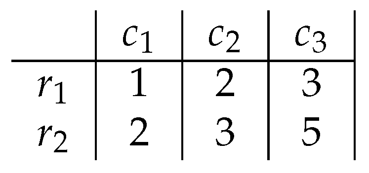
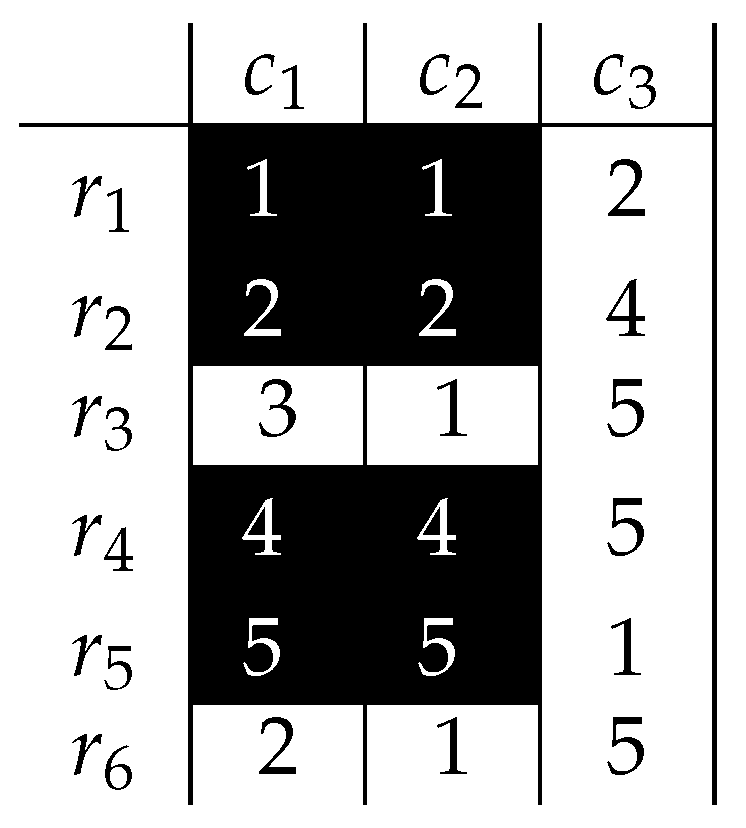
In order to illustrate how the Boolean reasoning can help finding biclusters, a simple example will be shown. The maximal absolute difference between any two cells in matrix (Figure 3) is equal to 4. The greatest absolute difference smaller than 4 is 3. The Boolean function, encoding the data, is a conjunction of clauses whose variables correspond to rows and columns of two cells that differ by more than 3. The only pair of cells whose difference exceeds 3 is and . The Conjunctive Normal Form (CNF) clause that encodes these cells with the row and column’s corresponding Boolean variables is . This clause is already in Disjunctive Normal Form (DNF) and consists of four prime implicants.
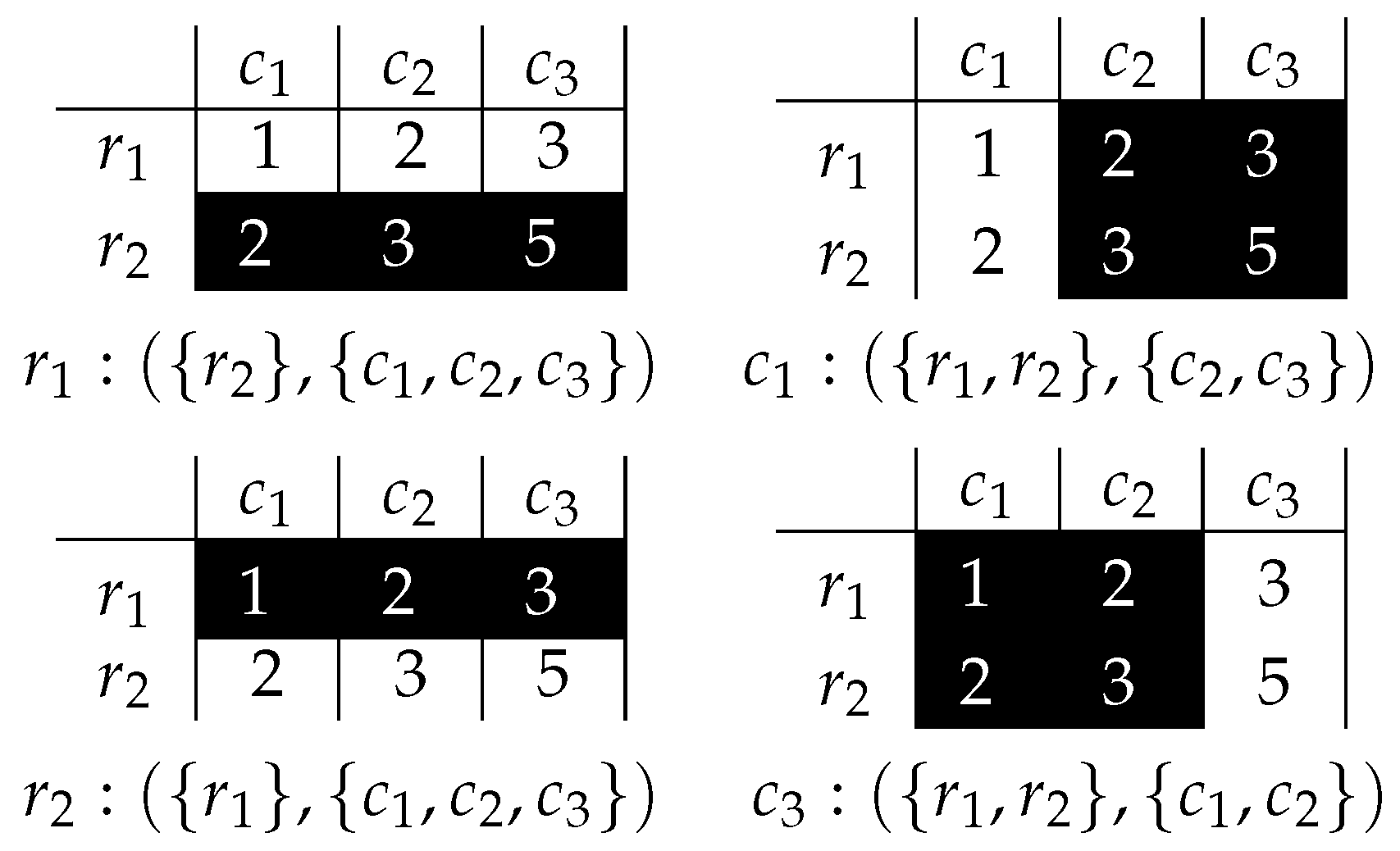
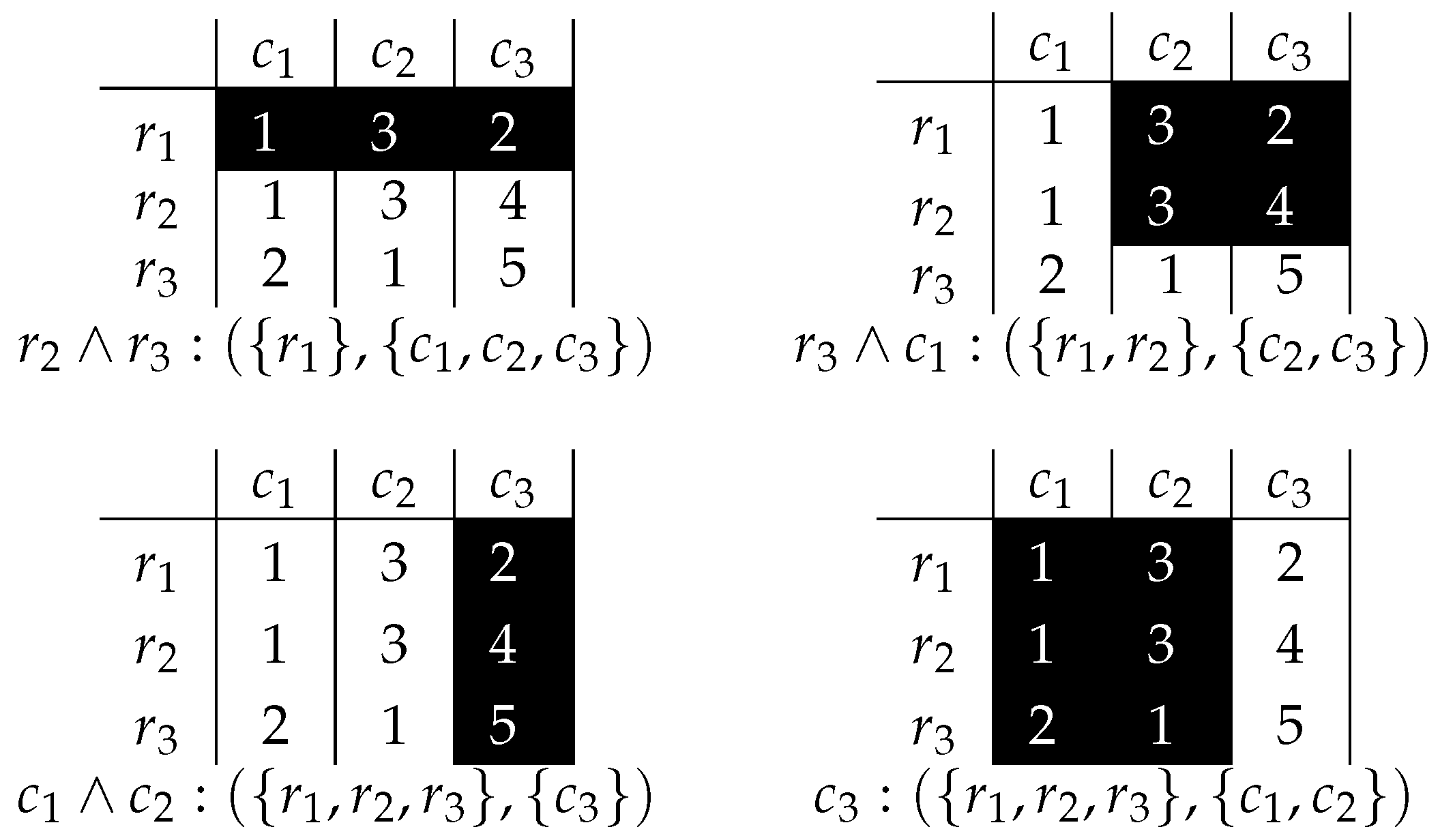
It was proven that biclusters associated with prime implicants are defined by variables that are not present in the prime implicants. From matrix and the function (pairs exceeding the value 3), several biclusters can be provided, as shown in Figure 4.
For example, the first implicant is , which corresponds to the bicluster formed by all the columns, and only the row . Also, there is neither a column nor a row that can be added to the bicluster without violating the defined property on the maximal absolute difference. The example reveals that it is possible to express global properties of biclusters in terms of Boolean reasoning. However, it becomes interesting to analyze only in-row absolute differences instead of global ones, as it implicitly considers the order of rows, what has important consequences for the analysis of data in several domains (e.g., venereal tumors [40], time-lagged data [41]).
The previous approach was successfully developed for finding constant biclusters in discrete and binary data [37] so as for finding biclusters of similar values in continuous data [42]. This work extends the research to address the search for biclusters in continuous data that include more sophisticated patterns (not only constant real values), and it requires new definitions, proofs and the methodology to validate the approach in the context of real-world problems.
4. Pattern Induction with Boolean Reasoning
The definitions to support the procedure of extracting biclusters in real-valued domains by means of Boolean reasoning will be presented next.
4.1. Constant Patterns
Definition 6
(Constant pattern) The bicluster is a constant pattern of matrix if and it satisfies .
Figure 5 presents the matrix of continuous values, containing the constant pattern , which has the same value for a subset of columns. Moreover, there are neither rows nor columns that can be added without violating the condition of inclusion-maximality (see Definition 3).
Boolean reasoning can help with finding all the patterns by defining the function that encodes all the pairs of cells (at each row independently) with different values.
Definition 7
(Boolean function that encodes all in-row absolute differences). Let be a matrix of rows and columns . The Boolean function that encodes all in-row pairs with different values is defined as follows:
where
such that
For the matrix in Figure 5, the Boolean function is:
and simplifying, in DNF:
The final form of has additionally introduced brackets for the better presentation of its prime implicants.
Prime implicants of the function encode the patterns in such a way that the pattern consists of both rows and columns whose corresponding Boolean variables are not present in the prime implicant.
The constant pattern shown in Figure 5 is easily identified by means of its prime implicant (), which is associated to the bicluster , in accordance to Definition 5. The first implicant and the last two and refer to single-column patterns. It might not be so intuitive that each column represents a pattern that only contains one column with all rows—although formally correct. Finally, the second implicant () refers to the empty pattern, which is still consistent with Definition 3.
The theorems that establish the relationship between implicants and constant patterns, and between prime implicants and inclusion-maximal constant patterns, respectively, are stated below.
Theorem 1
(Implicants and constant patterns). is an implicant of if is a constant pattern in .
Theorem 2
(Prime implicants and inclusion-maximal constant patterns). is a prime implicant of if is an inclusion-maximal constant pattern in .
The proofs of above theorems can be found in Appendix A.1.
4.2. -Shifting Patterns
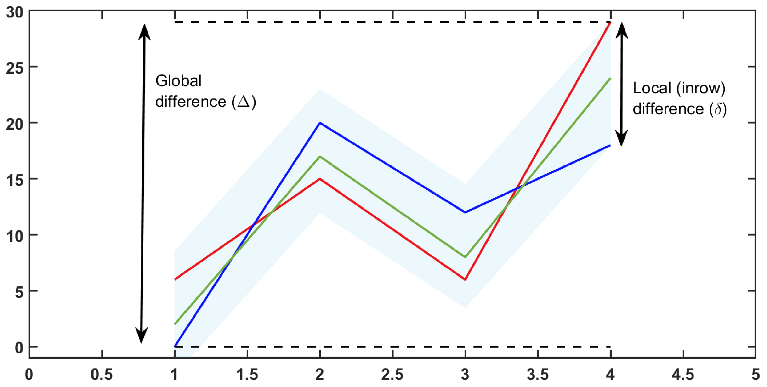
The shifting pattern is presented in Figure 2 as an analogy of shifting pattern in Figure 2. Each line of the pattern may be interpreted as the up–down shift of any of them. However, even a small change of any of the pattern series may cause the pattern to no longer be a shifting one. However, such a hidden pattern may be still of interest to the data owner. That leads us to the idea of the -shifting pattern that contains series that do not exceed a given threshold () of the difference between rows. A simple visualization is provided in Figure 6. The overall fluctuation of the pattern, containing three: red, green and blue lines, is , although it is more relevant to focus on the local fluctuation for each experimental condition illustrated by the blue shaded band whose difference is .
The concept of shifting pattern was introduced in Section 2.2, and it can be formally generalized in order to consider that the maximal absolute in-row difference between pairs of cells will not exceed a given threshold .
Definition 8
(-Shifting Pattern). A bicluster shows a-shifting pattern when:
It becomes intuitive (from the relationship between Definitions 6 and 7) that proper Boolean functions should be based on the negation of the condition in Equation (1)—the encoding of all in-row pairs that violate this condition.
Definition 9
(Boolean function that encodes all in-row absolute differences greater than ). Let be a matrix of rows and columns . The Boolean function that encodes all in-row pairs whose difference is not greater than δ is defined as follows:
where
such that
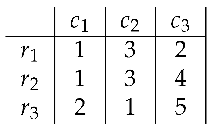
Figure 7 shows the matrix with three rows and three columns. To build the formula (to find inclusion-maximal -shifting patterns), all the pairs of cells whose absolute difference exceeds the value 2 should be found (at each row separately). The first row does not contain such pairs, so it does not generate any clause. There is one pair in the second row and whose absolute difference is 3. Such a pair is encoded with a disjunction of three Boolean variables that correspond to the row (2) and to the columns (1 and 3), so the clause has the following form: . All clauses are logically multiplied, so the final CNF expression looks as follows:
Transforming the CNF function into DNF would discover the presence of interesting prime implicants encoding -shifting patterns:
Finally, four prime implicants were found (Figure 8) associated with biclusters that are inclusion-maximal -shifting patterns and whose row differences do not exceed 2.
In short, it is possible to express the -shifting pattern induction in terms of Boolean reasoning-based functions, which is demonstrated in Theorems 3 and 4.
Theorem 3
(Implicants and -shifting patterns). is an implicant of if is a δ-shifting pattern in .
Theorem 4
(Prime implicants and inclusion-maximal -shifting patterns). is a prime implicant of if is an inclusion-maximal δ-shifting pattern in .
The proofs of the above theorems can be found in Appendix A.2.
The presented approach limits the search for patterns, since it depends on the choice of the value. The next subsection will provide strategies that avoid such a constraint.
5. Experimental Analysis
In order to show the quality of results, we have selected a well-known dataset related to central nervous system development, which consists of 9 conditions and 112 genes [43]. Genes were clustered into related expression patterns to infer regulatory origins and interactions between families across the transition of the rat cervical spinal cord from a primary to a highly differentiate state, which is determined by embryonic days 11 through 21 (E11–E21), postnatal days 0–14 (P0–P14), and adult (A) at 90 days. This work was one of the first to suggest that similarities in expression patterns might point to the existence of common regulatory structures, which is useful in defining roles for genes with unknown functions. The choice of the dataset is justified by its features to show empirically the validity of the proposed methodology, focusing on the quality of the results from the analytical perspective without elaborating on their biological interpretation.
The core experiments were performed as a Boolean reasoning-based constant and -shifting pattern induction. To emphasize the advantages of such an approach, the results of other biclustering techniques are also presented.
It is noteworthy that for such an exhaustive approach based on Theorems 2 and 4, there is no need to know the ground true position of patterns (which is very common in other approaches like [44] or [45]). An artificially inserted -shifting pattern into random data will always be found, or even better, an extension of the original pattern.
5.1. Boolean Reasoning-Based Experiments
A first analysis was conducted to visualize the distribution of all in-row absolute differences. Figure 9 shows the distribution (histogram) for all the 55,944 pairs, which provide 2667 unique differences, ranging from 0 (minimum) to 27.69 (maximum) with a mean of 0.88. About 8% of differences are not greater than 0.1, while 15% are greater than 0.2, 22% are greater than 0.3, and almost 55% do not exceed 1.0. This suggests that the range [0,0.4] for is very reasonable for further evaluation, as it is covering more than of the pairs.
For , a total of 257 constant patterns were discovered, including one empty pattern and 112 single-column ones (each one of them containing all the rows). These two special cases (empty and single-column) are always discovered—when they exist—by the methodology, as Boolean reasoning also considers these patterns as biclusters (theoretically they are indeed). From this point, these patterns will be omitted for greater values of , and we will focus on patterns with at least two rows and two columns, as they seem to be the smallest patterns that generalize interesting properties in both dimensions. Taking this into account, there are 27 constant patterns in data.
For , we discovered 1027 patterns, and these can fluctuate within that difference, behaving as shifting patterns. For , the number of patterns increases up to 2487, for , it increases up to 4027, and for , it increases up to 6943. The quality of biclusters was measured to ensure that an increase in size does not necessarily lead to a decrease in quality. As a balanced measure of size, we will use the harmonic diameter (d), defined as , where r and c are the number of rows and columns of the bicluster, respectively. This measure reflects partially the shape of the pattern. Patterns with similar (or comparable) areas may have quite different harmonic diameters. For instance, three patterns with an area equal to 20 ( and ) will have their d values equal to 1.9, 3.33, and 4.44, respectively. However, the third one has the highest generalization ability.
The Mean Squared Residue () has been chosen as a measure of quality for biclusters because it is able to identify correctly constant and shifting patterns in data [4,14]. A low value (close to 0) means that the shifting pattern has no noise, and a high value means that either the shifting pattern has much noise or it is involved in a more complex pattern (e.g., a scaling pattern).
Table 1 summarizes the results of biclusters containing shifting patterns obtained by varying the value of . The maximum values of the Mean Squared Residue and harmonic diameter are also shown, and there is no significant loss of quality measured by the while the value of increases.
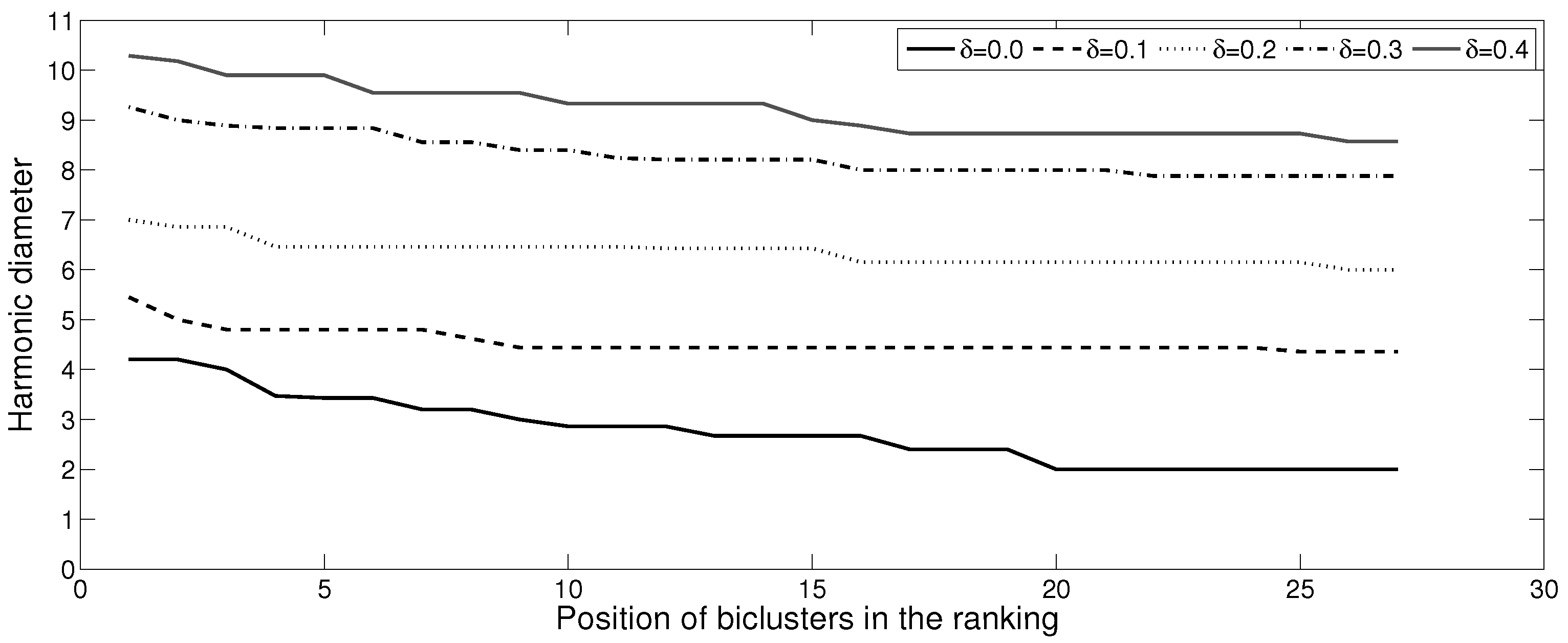
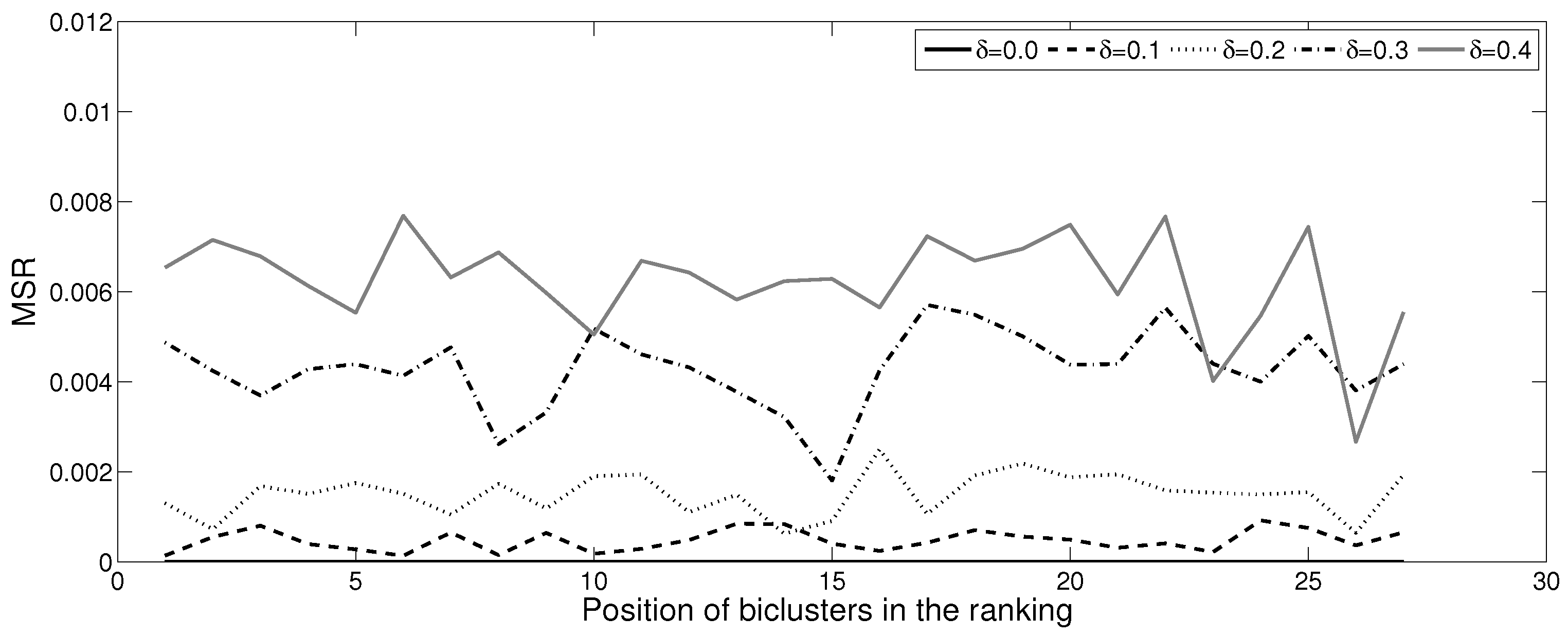
As only 27 meaningful patterns were found for (constant patterns), we have further limited the number of comparisons for the next values of with the goal of illustrating the good performance of the methodology regarding the size of biclusters (Figure 10). However, this increase in size has no negative effect on the quality of patterns, since the values of oscillate very little when the harmonic diameter increases (Figure 11), which remains very close to zero. Moreover, the level of of these 27 patterns is several times less than the maximal values presented in Table 1. In Figure 10 and Figure 11, the biclusters were decreasingly ordered by the harmonic diameter, so the X-axis represents the position of the bicluster in the ranking.
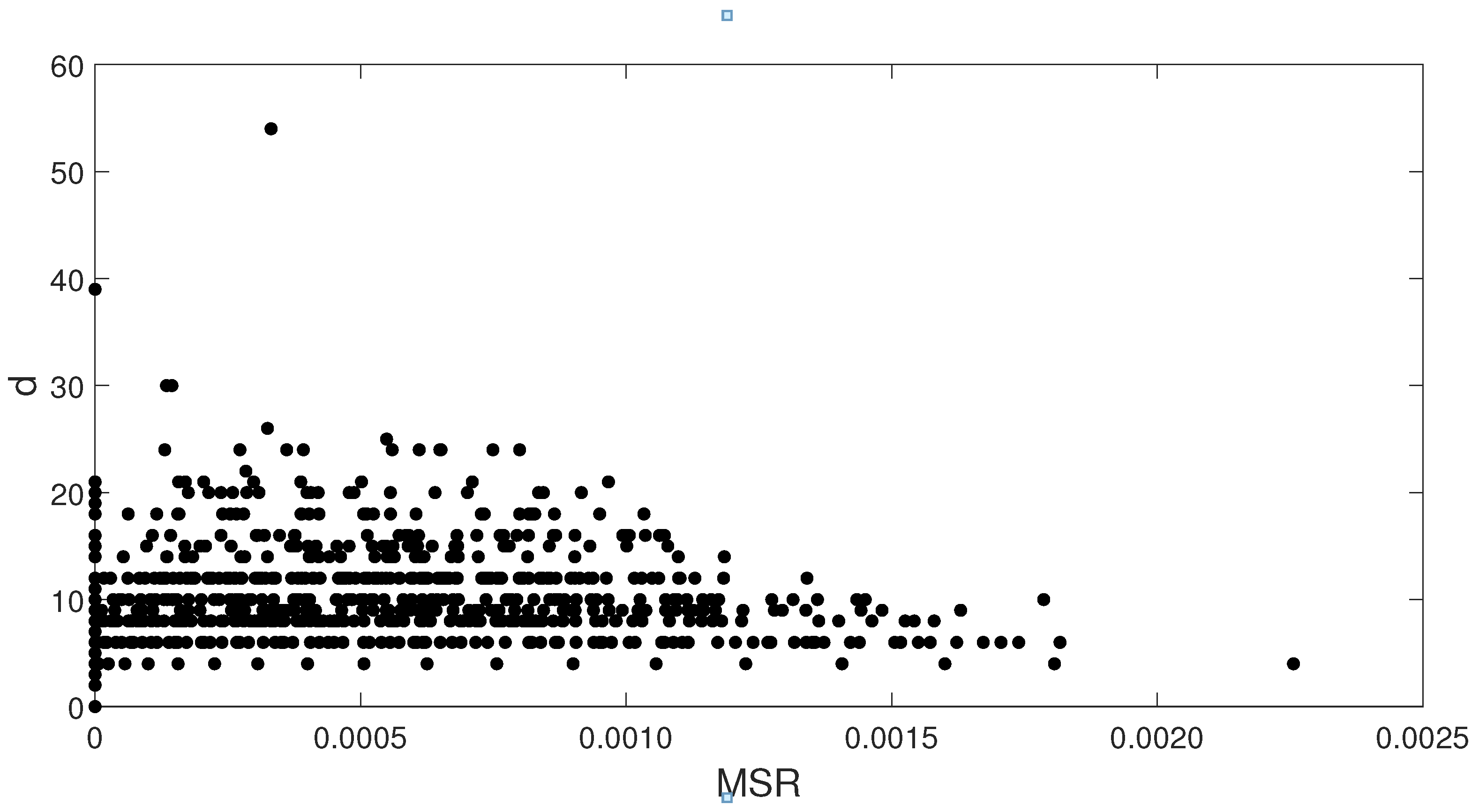
There exists a stable relationship between and d, since the variations in d do not necessarily lead to the same behavior in for (Figure 12). Thus, higher values of do not correspond to higher values of d, which suggests that larger patterns still have consistent in-row values, and this also occurs for greater values of .
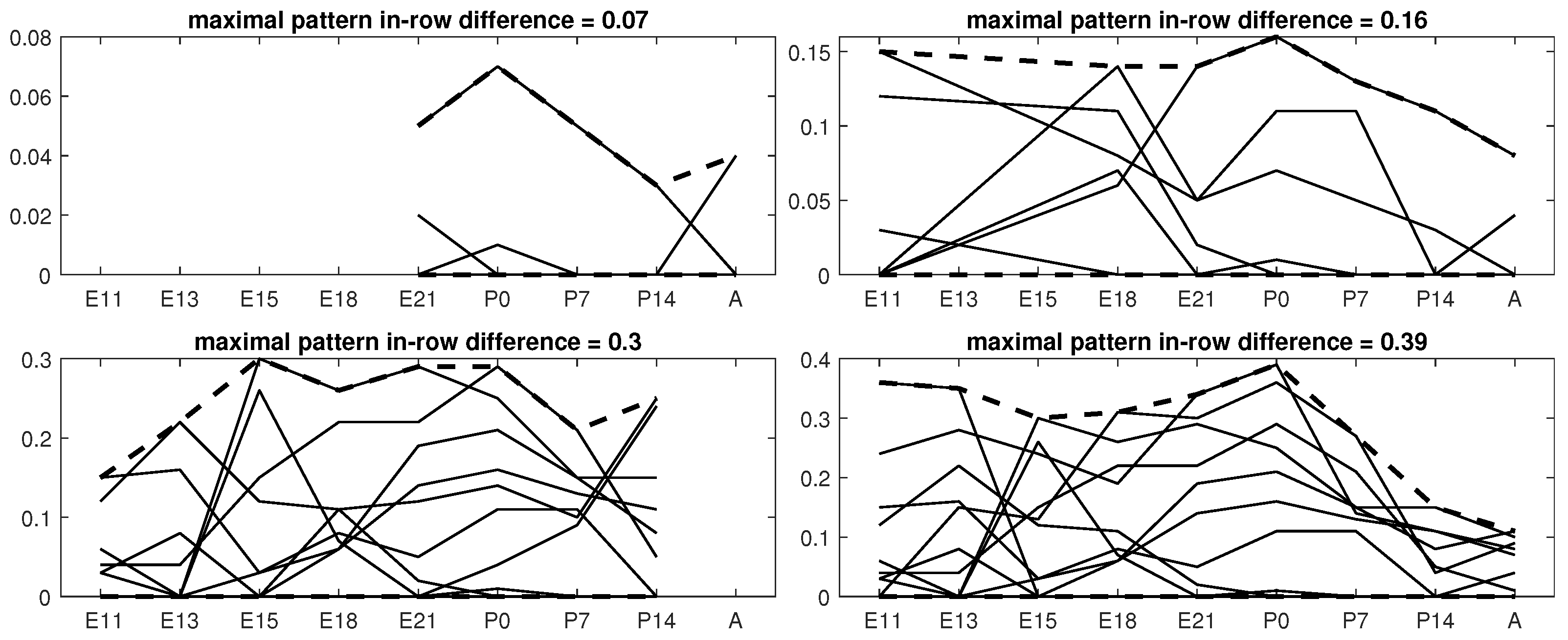
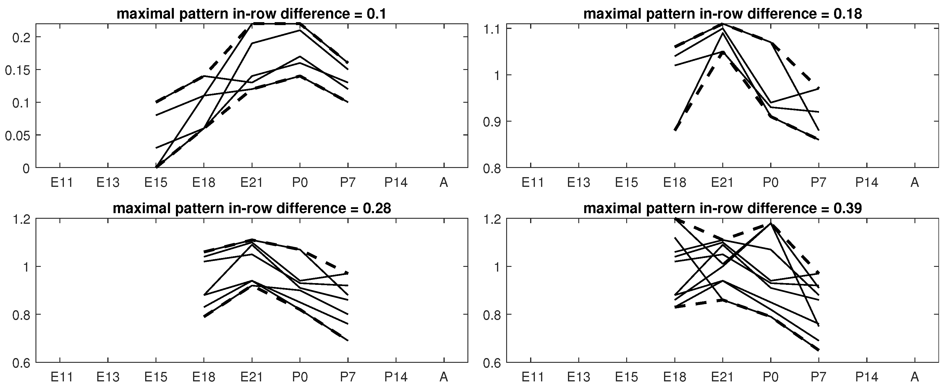
Examples of results for each value of will be shown in Figure 13 and Figure 14. Solid lines represent the behavior of each gene through the conditions. Additionally, the upper and lower bound of the pattern is marked with thicker dotted lines. The title of each subfigure indicates the maximal in-row difference of the pattern, which must be less than or equal to the value. A table is associated with each figure, in which details for each bicluster are presented.
The first group (Figure 13) shows the best bicluster (in terms of ) for each value of . Complementary information on each bicluster is presented in Table 2. The sizes of biclusters are slightly bigger as the value of increases, although with no significant impact on its quality, as the remains very close to zero. In this case, all the values within biclusters are very low, so it is not possible to appreciate great oscillations in behavior.
The approach does not only find biclusters whose lower bounds of the conditions are close to 0. The second group (Figure 14) shows four other biclusters with high fluctuations across the experimental conditions, which reveals important aspects related to gene regulation. The quality of biclusters (Table 3), measured by the , still remains very close to 0.
It is important to highlight that the lowest score indicates that the values fluctuate in unison with constant or shifting patterns. The values of calculated for the patterns presented in the previous tables are extremely low, taking into account that for a bicluster with values randomly and uniformly generated in the range of , the expected variance is . The ranges for the conditions vary from [0, 5.59] (E13) up to [0 27.69] (A), all of them starting from zero, so the expected is much higher than those depicted in Table 1 and thereby in Table 2 and Table 3.
There exist common rows and columns for two patterns, so their intersection is not an empty set (patterns overlap each other partially). Biclusters only focus on patterns (locally) and not on partitions (globally) as clusters. This is also noticed in the solutions: the eight biclusters displayed in both Figure 13 and Figure 14 use 61 rows (genes) in total; however, they only contain 27 unique rows. Irrelevant rows or columns would never appear in the solutions, satisfying the second property.
Finally, although it is out of the scope of this work to biologically analyze the quality of patterns, it is a general feature—extendable to other domains—that the behavior of genes (lines in the figures) presents fluctuations, which might reveal up- or down-regulation. This characteristic can be measured by the range coverage in terms of percentage, as this aspect is not usually illustrated in figures. For example, the bicluster displayed in Figure 14 for (bottom left) contains seven genes (lines), representing the behavior of those genes for four experimental conditions. Each gene has an original range of values, and it is desirable that the pattern contains a great part of that range, as it would include fluctuations instead of a flat behavior. The range coverage of that bicluster is, for each gene, 24.2%, 23.5%, 40%, 31.7%, 17.1%, 30.7%, and 10.1%, respectively, which indicates that when only using four out of nine experimental conditions, the pattern is substantially varying across the original range.
5.2. Biological Interpretation
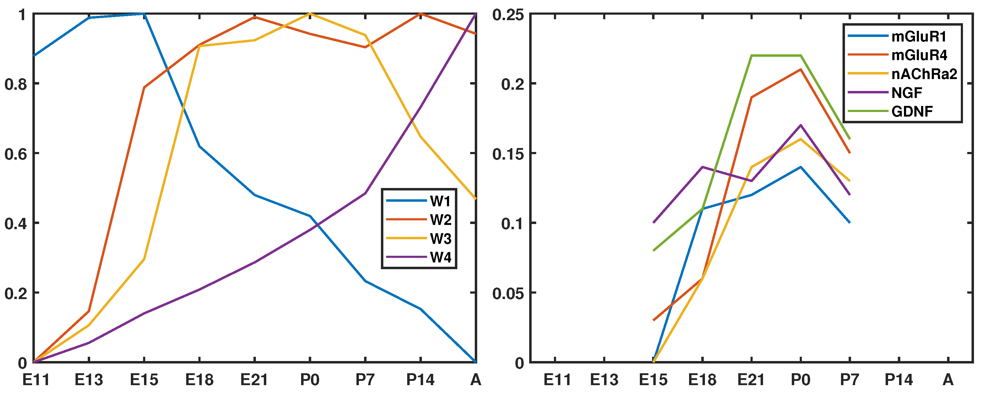
Originally, the 112 genes were grouped into four functional categories: Neuro-Grial Markers, Neurotransmitter Receptors, Peptide Signaling, and Diverse. A further inspection of data pointed out relationships between signaling gene families, providing six groups according to the averaged behavior across all the conditions (from E11 to A): four waves (W1–W4) characterizing distinct phases of development, a constant pattern, and the last group named other (six genes with no common behavior and not related to the other groups). In short, two types of clustering were taken into account by Wen et al. [43]: signaling gene families (without analyzing data) and pattern-based gene families (only observing the data for all the conditions). Genes fluctuating in parallel for specific temporal conditions could help understand the nature of complex developmental and degenerative disorders.
In order to highlight the usefulness of our approach, the solution provided in Figure 14 for = (upper left) reveals that it is possible to group genes with no signaling relationships and, above all, that were not grouped into any of the waves. Therefore, some genes from different functional categories could follow a pattern from a subset of experimental conditions (E15–P7) that were not identified in previous research because they do not share the same global pattern, i.e., waves depicted in Figure 15 (left). The bicluster illustrated in Figure 15 (right) suggests that there is a close correspondence in terms of coexpression of metabotropic glutamate and nicotinic acetylcholine receptors as well as glial-derived neurotrophic and nerve growth factors. This aspect motivates further biological research on why these functionally different genes, not present together in the same wave, are coexpressing within a certain time interval.
Our approach is able to find all existing -shifting patterns in the data. For instance, as shown in Table 1, the number of patterns extracted from data for equal to is 6943, each of which must be biologically validated (via public web services) to identify the most relevant ones related to biological mechanisms (common regulatory structures and pathways). On the other hand, most biclustering techniques do not provide all possible biclusters or, on the contrary, they are limited to a certain number of results. This situation would lead to a loss of potentially meaningful patterns from a biological validation perspective.
5.3. Comparative Analysis
Methods provided by the biclust package [46] for the R environment [47] were chosen. According to [4], we tried to find one pattern corresponding to the value from Table 2. That meant that for each search, a corresponding limit () should be used separately. The summary of results is presented in Table 4.
Taking into consideration the for the largest (in terms of d measure) results from Table 2, it must be stated that for the , the found pattern is much smaller () than the one found by the Boolean reasoning-based approach (). Moreover, there was still much space for pattern extension as its was equal to 0.02 and the limitation was 0.1. In the case of the second search, the patterns were comparable ( vs. ). However, the pattern found by the Boolean reasoning strategy had one more condition. For the next two cases, we observe that larger patterns do not follow the required constrain: 0.36 instead of 0.30 and 0.44 instead of 0.40. Concluding, searching for the -shifting pattern with the Cheng and Church strategy is not a suitable tool for such a purpose: the found patterns are smaller or its values exceed the required level for .
Another comparison was carried out with the Plaid Model biclustering [48] (the improved version of the approach presented in [49]). The pattern found with default parameters has only four genes and three conditions and . Changing the values of several method parameters such that max.layers as well as background, iter.startup, and iter.layer did not provide any better results as mentioned above. Concluding, finding -shifting patterns with this tool is even much more difficult than with the Cheng and Church approach.
Finally, the approach presented in [50], with the parameter setting proposed in [46], only provided a constant pattern of zeros (three genes and seven conditions), which is easily found by the Boolean reasoning approach. Many different parameter settings were not able to improve this result or even provided none bicluster.
6. Conclusions and Further Works
In this work, the problem of biclustering on real-valued data from the Boolean reasoning perspective is addressed. A new definition of pattern in continuous data is provided as well as how to search for them in terms of Boolean reasoning. Mathematical foundations are provided to support the use of Boolean concepts, in particular, the maximal-inclusion patterns, in the search for biclusters that include -shifting patterns.
While most algorithms use heuristic strategies to cope with the complexity of the biclustering problem and find biclusters that represent good (though not all) solutions, the presented approach always finds all the inclusion-maximal solutions for the threshold set for the -shifting pattern. Moreover, the presented theorems open the gates to some heuristic strategies for non-prime-implicant search, as the corresponding patterns will still have some of the desired properties but might not be inclusion-maximal, as it has already been pointed out [51,52].
Experiments on central nervous system development data suggest that the approach has excellent performance (measured by the mean squared residue) at finding large fluctuations of rows across columns (or vice versa) while maintaining small fluctuations of columns (or rows).
Finally, future research directions will tackle the search for scaling patterns, for which it has been already proven that the mean squared residue is not an appropriate measure to score the quality of patterns, especially when combined with shifting patterns.
Author Contributions
Conceptualization, M.M. and J.S.A.-R.; methodology, M.M.; software, M.M.; validation, M.M. and J.S.A.-R.; formal analysis, M.M.; investigation, M.M. and J.S.A.-R.; resources, M.M. and J.S.A.-R.; data curation, M.M. and J.S.A.-R.; writing—original draft preparation, M.M. and J.S.A.-R.; writing—review and editing, M.M. and J.S.A.-R.; visualization, M.M.; supervision, M.M. and J.S.A.-R.; project administration, M.M. and J.S.A.-R.; funding acquisition, M.M. All authors have read and agreed to the published version of the manuscript.
Funding
This work was supported by Grant PID2020-117759GB-I00 funded by MCIN/AEI/10.13039/501100011033, the Andalusian Plan for Research, Development and Innovation and the Department of Computer Networks and Systems (RAu9) at Silesian University of Technology.
Data Availability Statement
Conflicts of Interest
The authors declare no conflict of interest.
Appendix A. Theorems and Proofs
Appendix A.1. Proofs of Theorems for Constant Pattern Induction
Proof of Theorem 1.
(Implicants and constant patterns) is an implicant of if is a constant pattern in . □
⇒ Let be an implicant of and be not a constant pattern in . That means that there exists at least one pair of different columns and a row such that:
This in turn means that the clause is not satisfied by , which introduces the contradiction with the assumption.
⇐ Let be a constant pattern in and be not an implicant in . That means that there exists and such that
which makes the contradiction.
Proof of Theorem 2.
(Prime implicants and inclusion-maximal constant patterns) is a prime implicant of if is an inclusion-maximal constant pattern in . □
⇒ Let be a prime implicant of and be not an inclusion-maximal constant pattern in . That means that there exists at least one column or row such that or is also a constant pattern. However, on the basis of Theorem 1, or is also an implicant of , so cannot be the prime implicant, and it is in contradiction to the assumptions.
⇐ Let be an inclusion-maximal constant pattern in and be not a prime implicant in . That would mean that there exists or such that or is also an implicant of . This in turn means (Theorem 1) that or will be an inclusion-maximal constant pattern in , which makes a contradiction.
Appendix A.2. Proofs of Theorems for δ-Shifting Pattern Induction
Proof of Theorem 3.
(Implicants and -shifting patterns) is an implicant of if is a -shifting pattern in . □
⇒ Let be an implicant of and be not a -shifting pattern in . That means that there exists at least one pair of different columns and a row r such that:
This in turns means that the clause is not satisfied by , which introduces the contradiction with the assumption.
⇐ Let be a -shifting pattern in and be not an implicant in . That means that there exists and such that
which makes the contradiction.
Having proved the Theorem 3, it is possible to prove Theorem 4.
Proof of Theorem 4.
(Prime implicants and inclusion-maximal -shifting patterns) is a prime implicant of if is an inclusion-maximal -shifting pattern in . □
⇒ Let be a prime implicant of and be not an inclusion-maximal -shifting pattern in . That means that there exists at least one column or row such that or is also a -shifting pattern. However, on the basis of Theorem 3, or is also an implicant of , so cannot be the prime implicant, and it is in contradiction to the assumptions.
⇐ Let be an inclusion-maximal -shifting pattern in and be not a prime implicant in . That would mean that there exists or such that or is also an implicant of . This in turn means (Theorem 3) that or will be a -shifting pattern bicluster in , which makes a contradiction.
References
- Morgan, J.; Sonquist, J. Problems in the analysis of survey data, and a proposal. J. Am. Stat. Assoc. 1963, 58, 415–434. [Google Scholar] [CrossRef]
- Hartigan, J.A. Direct clustering of a data matrix. J. Am. Stat. Assoc. 1972, 67, 123–129. [Google Scholar] [CrossRef]
- Mirkin, B. Mathematical Classification and Clustering; Kluwer: Alphen aan den Rijn, The Netherlands, 1996. [Google Scholar]
- Cheng, Y.; Church, G.M. Biclustering of Expression Data. In Proceedings of the Eighth International Conference on Intelligent Systems for Molecular Biology; AAAI Press: Washington, DC, USA, 2000; pp. 93–103. [Google Scholar]
- Tanay, A.; Sharan, R.; Shamir, R. Discovering statistically significant biclusters in gene expression data. Bioinformatics 2002, 18, S136–S144. [Google Scholar] [CrossRef]
- Fernández, D.; Sram, R.J.; Dostal, M.; Pastorkova, A.; Gmuender, H.; Choi, H. Modeling Unobserved Heterogeneity in Susceptibility to Ambient Benzo[a]pyrene Concentration among Children with Allergic Asthma Using an Unsupervised Learning Algorithm. Int. J. Environ. Res. Public Health 2018, 15, 106. [Google Scholar] [CrossRef]
- Silva, M.G.; Madeira, S.C.; Henriques, R. Water Consumption Pattern Analysis Using Biclustering: When, Why and How. Water 2022, 14, 1954. [Google Scholar] [CrossRef]
- Yazdanparast, A.; Li, L.; Zhang, C.; Cheng, L. Bi-EB: Empirical Bayesian Biclustering for Multi-Omics Data Integration Pattern Identification among Species. Genes 2022, 13, 1982. [Google Scholar] [CrossRef]
- Chagoyen, M.; Carmona-Saez, P.; Shatkay, H.; Carazo, J.M.; Pascual-Montano, A. Discovering semantic features in the literature: A foundation for building functional associations. BMC Bioinform. 2006, 7, 41. [Google Scholar] [CrossRef] [PubMed]
- Orzechowski, P.; Boryczko, K. Text Mining with Hybrid Biclustering Algorithms. Lect. Notes Comput. Sci. 2016, 9693, 102–113. [Google Scholar]
- Busygin, S.; Prokopyev, O.; Pardalos, P.M. Biclustering in data mining. Comput. Oper. Res. 2008, 35, 2964–2987. [Google Scholar] [CrossRef]
- Pontes, B.; Giráldez, R.; Aguilar-Ruiz, J.S. Biclustering on expression data: A review. J. Biomed. Inform. 2015, 57, 163–180. [Google Scholar] [CrossRef]
- Madeira, S.C.; Oliveira, A. Biclustering algorithms for biological data analysis: A survey. IEEE/ACM Trans. Comput. Biol. Bioinform. 2004, 1, 24–45. [Google Scholar] [CrossRef] [PubMed]
- Aguilar-Ruiz, J.S. Shifting and scaling patterns from gene expression data. Bioinformatics 2005, 21, 3840–3845. [Google Scholar] [CrossRef] [PubMed]
- Ahmed, H.; Mahanta, P.; Bhattacharyya, D.; Kalita, J. Shifting-and-scaling correlation based biclustering algorithm. IEEE/ACM Trans. Comput. Biol. Bioinform. 2014, 11, 1239–1252. [Google Scholar] [CrossRef] [PubMed]
- Bryan, K.; Cunningham, P.; Bolshakova, N. Application of Simulated Annealing to the Biclustering of Gene Expression Data. IEEE Trans. Inf. Technol. Biomed. 2006, 10, 519–525. [Google Scholar] [CrossRef] [PubMed]
- Bryan, K.; Cunningham, P. Extending bicluster analysis to annotate unclassified ORFs and predict novel functional modules using expression data. BMC Genom. 2008, 9, S20. [Google Scholar] [CrossRef]
- Reiss, D.J.; Baliga, N.S.; Bonneau, R. Integrated biclustering of heterogeneous genome-wide datasets for the inference of global regulatory networks. BMC Bioinform. 2006, 7, 280. [Google Scholar] [CrossRef]
- Alzahrani, M.; Kuwahara, H.; Wang, W.; Gao, X. Gracob: A novel graph-based constant-column biclustering method for mining growth phenotype data. Bioinformatics 2017, 33, 2523–2531. [Google Scholar] [CrossRef]
- Karim, M.B.; Huang, M.; Ono, N.; Kanaya, S.; Altaf-Ul-Amin, M. BiClusO: A novel biclustering approach and its application to species-VOC relational data. IEEE/ACM Trans. Comput. Biol. Bioinform. 2020, 17, 1955–1965. [Google Scholar] [CrossRef]
- Li, G.; Ma, Q.; Tang, H.; Paterson, A.H.; Xu, Y. QUBIC: A qualitative biclustering algorithm for analyses of gene expression data. Nucleic Acids Res. 2009, 37, e101. [Google Scholar] [CrossRef]
- Denitto, M.; Farinelli, A.; Figueiredo, M.; Bicego, M. A biclustering approach based on factor graphs and the max-sum algorithm. Pattern Recognit. 2017, 62, 114–124. [Google Scholar] [CrossRef]
- Denitto, M.; Bicego, M.; Farinelli, A.; Figueiredo, M. Spike and slab biclustering. Pattern Recognit. 2017, 72, 186–195. [Google Scholar] [CrossRef]
- Kluger, Y.; Basri., R.; Chang, J.T.; Gerstein, M. Spectral biclustering of microarray data: Coclustering genes and conditions. Genome Res. 2003, 13, 703–716. [Google Scholar] [CrossRef]
- Mitra, S.; Banka, H. Multi-objective evolutionary biclustering of gene expression data. Pattern Recognit. 2006, 39, 2464–2477. [Google Scholar] [CrossRef]
- Hanczar, B.; Nadif, M. Ensemble methods for biclustering tasks. Pattern Recognit. 2012, 45, 3938–3949. [Google Scholar] [CrossRef]
- Nepomuceno, J.A.; Troncoso, A.; Aguilar-Ruiz, J.S. Biclustering of Gene Expression Data by Correlation-Based Scatter Search. BioData Min. 2011, 4, 3. [Google Scholar] [CrossRef]
- Banerjee, A.; Dhillon, I.; Ghosh, J.; Merugu, S.; Modha, D.S. A Generalized Maximum Entropy Approach to Bregman Co-clustering and Matrix Approximation. J. Mach. Learn. Res. 2007, 8, 1919–1986. [Google Scholar]
- Gupta, N.; Aggarwal, S. MIB: Using mutual information for biclustering gene expression data. Pattern Recognit. 2010, 43, 2692–2697. [Google Scholar] [CrossRef]
- Pontes, B.; Giráldez, R.; Aguilar-Ruiz, J. Quality Measures for Gene Expression Biclusters. PLoS ONE 2015, 10, e0115497. [Google Scholar] [CrossRef]
- Flores, J.L.; Inza, I.; Larrañaga, P.; Calvo, B. A new measure for gene expression biclustering based on non-parametric correlation. Comput. Methods Programs. Biomed. 2013, 112, 367–397. [Google Scholar] [CrossRef]
- Wille, R. Restructuring Lattice Theory: An Approach Based on Hierarchies of Concepts. In Proceedings of the Ordered Sets, Banff, AB, Canada, 28 August–12 September 1981; Rival, I., Ed.; Springer: Berlin/Heidelberg, Germany, 1982; pp. 445–470. [Google Scholar]
- Serin, A.; Vingron, M. DeBi: Discovering Differentially Expressed Biclusters using a Frequent Itemset Approach. Algorithms Mol. Biol. 2011, 6, 18. [Google Scholar] [CrossRef] [PubMed]
- Aguinis, H.; Forcum, L.E.; Joo, H. Using Market Basket Analysis in Management Research. J. Manag. 2013, 39, 1799–1824. [Google Scholar] [CrossRef]
- Tomescu, M.A.; Jäntschi, L.; Rotaru, D.I. Figures of Graph Partitioning by Counting, Sequence and Layer Matrices. Mathematics 2021, 9, 1419. [Google Scholar] [CrossRef]
- Brown, F.M. Boolean Reasoning; Springer: New York, NY, USA, 1990. [Google Scholar]
- Michalak, M.; Ślȩzak, D. Boolean Representation for Exact Biclustering. Fundam. Inform. 2018, 161, 275–297. [Google Scholar] [CrossRef]
- José-García, A.; Jacques, J.; Sobanski, V.; Dhaenens, C. Metaheuristic Biclustering Algorithms: From State-of-the-Art to Future Opportunities. ACM Comput. Surv. 2023, 56, 1–38. [Google Scholar] [CrossRef]
- van Uitert, M.; Meuleman, W.; Wessels, L.F.A. Biclustering Sparse Binary Genomic Data. J. Comput. Biol. 2008, 15, 1329–1345. [Google Scholar] [CrossRef]
- Chokeshaiusaha, K.; Puthier, D.; Nguyen, C.; Sudjaidee, P.; Sananmuang, T. Factor Analysis for Bicluster Acquisition (FABIA) revealed vincristine-sensitive transcript pattern of canine transmissible venereal tumors. Heliyon 2019, 5, e01558. [Google Scholar] [CrossRef]
- Gonçalves, J.P.; Madeira, S.C. LateBiclustering: Efficient Heuristic Algorithm for Time-Lagged Bicluster Identification. IEEE/ACM Trans. Comput. Biol. Bioinform. 2014, 11, 801–813. [Google Scholar] [CrossRef]
- Michalak, M. Induction of Centre—Based Biclusters in Terms of Boolean Reasoning. Adv. Intell. Syst. Comput. 2020, 1061, 239–248. [Google Scholar]
- Wen, X.; Fuhrman, S.; Michaels, G.S.; Carr, D.B.; Smith, S.; Barker, J.L.; Somogyi, R. Large-scale temporal gene expression mapping of central nervous system development. Proc. Natl. Acad. Sci. USA 1998, 95, 334–339. [Google Scholar] [CrossRef]
- Wang, Z.; Li, G.; Robinson, R.W.; Huang, X. UniBic: Sequential row-based biclustering algorithm for analysis of gene expression data. Sci. Rep. 2016, 6, 23466. [Google Scholar] [CrossRef]
- Liu, X.; Li, D.; Liu, J.; Su, Z.; Li, G. RecBic: A fast and accurate algorithm recognizing trend-preserving biclusters. Bioinformatics 2020, 36, 5054–5060. [Google Scholar] [CrossRef] [PubMed]
- biclust: BiCluster Algorithms. Available online: https://cran.r-project.org/web/packages/biclust/index.html (accessed on 1 October 2023).
- R Core Team. R: A Language and Environment for Statistical Computing; R Foundation for Statistical Computing: Vienna, Austria, 2014. [Google Scholar]
- Turner, H.; Bailey, T.; Krzanowski, W. Improved biclustering of microarray data demonstrated through systematic performance tests. Comput. Stat. Data Anal. 2005, 48, 235–254. [Google Scholar] [CrossRef]
- Lazzeroni, L.; Owen, A. Plaid Models for Gene Expression Data. Stat. Sin. 2002, 12, 61–86. [Google Scholar]
- Murali, T.M.; Kasif, S. Extracting Conserved Gene Expression Motifs from Gene Expression Data. In Proceedings of the Pacific Symposium Biocomputing, Kauai, HI, USA, 3–7 January 2003; pp. 77–88. [Google Scholar]
- Michalak, M.; Jaksik, R.; Ślȩzak, D. Heuristic Search of Exact Biclusters in Binary Data. Int. J. Appl. Math. Comput. Sci. 2020, 30, 161–171. [Google Scholar]
- Michalak, M. Hierarchical heuristics for Boolean-reasoning-based binary bicluster induction. Acta Inform. 2022, 59, 673–685. [Google Scholar] [CrossRef]
Figure 1.
Matrix presented as the set of column series.

Figure 2.
Shifting pattern within the data.

Figure 3.
A sample matrix .

Figure 4.
Biclusters identified by the prime implicants and the corresponding bicluster representation for matrix .
Figure 4.
Biclusters identified by the prime implicants and the corresponding bicluster representation for matrix .

Figure 5.
A sample matrix with a constant pattern.

Figure 6.
The -shifting pattern example.

Figure 7.
A sample matrix .

Figure 8.
Prime implicants of function .

Figure 9.
Histogram of all in-row absolute differences from data.

Figure 10.
Harmonic diameter of the 27 patterns ranked with highest d for every value of .

Figure 11.
of the 27 patterns ranked with the highest d for every value of .

Figure 12.
Relationship between the mean squared residue () and the harmonic diameter d for 0.1-shifting patterns.
Figure 12.
Relationship between the mean squared residue () and the harmonic diameter d for 0.1-shifting patterns.

Figure 13.
Best -shifting patterns (in terms of harmonic diameter) found for several levels of : (upper left), (upper right), (bottom left) and (bottom right). Upper and lower bound of the pattern is marked with thick dotted lines, while gene values through conditions are represented with thin solid lines.

Figure 14.
Additional -shifting patterns found for several levels of : (upper left), (upper right), (bottom left) and (bottom right). Solid lines represent the real pattern series while the dashed ones are boundaries of patterns.
Figure 14.
Additional -shifting patterns found for several levels of : (upper left), (upper right), (bottom left) and (bottom right). Solid lines represent the real pattern series while the dashed ones are boundaries of patterns.

Figure 15.
Four relevant waves identified by Wen et al. [43] (left); 0.1-shifting pattern provided by our approach (right).
Figure 15.
Four relevant waves identified by Wen et al. [43] (left); 0.1-shifting pattern provided by our approach (right).


Table 1.
Summary of -shifting patterns (not smaller than ) provided for several values of , including the highest value for the mean squared residue (worst case) and for the harmonic diameter.
Table 1.
Summary of -shifting patterns (not smaller than ) provided for several values of , including the highest value for the mean squared residue (worst case) and for the harmonic diameter.
| Number of Patterns | Max () | Max (d) | |
|---|---|---|---|
| 0.0 | 27 | 0.00000 | 4.20 |
| 0.1 | 1027 | 0.00226 | 5.45 |
| 0.2 | 2487 | 0.00951 | 7.00 |
| 0.3 | 4027 | 0.02102 | 9.26 |
| 0.4 | 6943 | 0.02976 | 10.29 |
Table 2.
Description of best -shifting patterns (in terms of harmonic diameter) for several levels of .
Table 2.
Description of best -shifting patterns (in terms of harmonic diameter) for several levels of .
| N. of Genes | N. of Cond. | Area | d | ||
|---|---|---|---|---|---|
| 6 | 5 | 30 | 0.00013 | 5.45 | |
| 7 | 7 | 49 | 0.00130 | 7.00 | |
| 11 | 8 | 88 | 0.00487 | 9.26 | |
| 12 | 9 | 108 | 0.00653 | 10.29 |
Table 3.
Description of other four -shifting patterns for several levels of .
| N. of Genes | N. of Cond. | Area | d | ||
|---|---|---|---|---|---|
| 5 | 5 | 25 | 0.00055 | 5.00 | |
| 4 | 4 | 16 | 0.00151 | 4.00 | |
| 4 | 7 | 28 | 0.00137 | 5.09 | |
| 4 | 9 | 36 | 0.00695 | 5.54 |
Table 4.
Results of Cheng and Church algorithm based on of widest results of Boolean reasoning-based approach and corresponding level of for a -shifting pattern.
Table 4.
Results of Cheng and Church algorithm based on of widest results of Boolean reasoning-based approach and corresponding level of for a -shifting pattern.
| N. of Genes | N. of Cond. | Area | d | ||
|---|---|---|---|---|---|
| 0.00013 | 3 | 5 | 15 | 0.02 | 3.75 |
| 0.00130 | 7 | 6 | 42 | 0.19 | 6.46 |
| 0.00487 | 14 | 8 | 112 | 0.36 | 10.18 |
| 0.00653 | 16 | 9 | 144 | 0.44 | 11.52 |
Disclaimer/Publisher’s Note: The statements, opinions and data contained in all publications are solely those of the individual author(s) and contributor(s) and not of MDPI and/or the editor(s). MDPI and/or the editor(s) disclaim responsibility for any injury to people or property resulting from any ideas, methods, instructions or products referred to in the content. |
© 2023 by the authors. Licensee MDPI, Basel, Switzerland. This article is an open access article distributed under the terms and conditions of the Creative Commons Attribution (CC BY) license (https://creativecommons.org/licenses/by/4.0/).
Share and Cite
MDPI and ACS Style
Michalak, M.; Aguilar-Ruiz, J.S. Shifting Pattern Biclustering and Boolean Reasoning Symmetry. Symmetry 2023, 15, 1977. https://doi.org/10.3390/sym15111977
AMA Style
Michalak M, Aguilar-Ruiz JS. Shifting Pattern Biclustering and Boolean Reasoning Symmetry. Symmetry. 2023; 15(11):1977. https://doi.org/10.3390/sym15111977
Chicago/Turabian StyleMichalak, Marcin, and Jesús S. Aguilar-Ruiz. 2023. "Shifting Pattern Biclustering and Boolean Reasoning Symmetry" Symmetry 15, no. 11: 1977. https://doi.org/10.3390/sym15111977
Note that from the first issue of 2016, this journal uses article numbers instead of page numbers. See further details here.