
Map Construction and Path Planning Method for Mobile Robots Based on Collision Probability Model

1
College of Geomatics and Geoinformation, Guilin University of Technology, Guilin 541004, China
2
Ecological Spatiotemporal Big Data Perception Service Laboratory, Guilin 541004, China
3
Guilin Agricultural Science Research Center, Guilin 541006, China
*
Author to whom correspondence should be addressed.
Symmetry 2023, 15(10), 1891; https://doi.org/10.3390/sym15101891
Submission received: 3 September 2023
/
Revised: 26 September 2023
/
Accepted: 29 September 2023
/
Published: 9 October 2023
(This article belongs to the Special Issue Computer Science and Symmetry/Asymmetry: Feature Papers)
Abstract
:A map construction method based on a collision probability model and an improved A* algorithm is proposed to address the issues of insufficient security in mobile robot map construction and path planning in complex environments. The method is based on modeling the asymmetry of paths, which complicates problem solving. Firstly, this article constructs a collision probability function model, and based on this model it is fused with the obstacle grid map, which is based on the grid method, to draw a collision probability grid map (CPGM) containing collision probability information. Secondly, incorporating the collision probability values from the CPGM into the actual cost function of the traditional A* algorithm improves the security of path planning in complex environments. The experimental results show that the improved A* algorithm decreases the percentage of dangerous nodes in complex environments by 69.23%, shortens the path planning length by 19.52%, reduces the search time by 16.8%, and reduces the number of turns by 46.67%. Therefore, the method in this paper solves the problem of traditional grid maps lacking security information and can plan a path with higher security and which is smoother, improving the security and robustness of mobile robot autonomous navigation in complex environments.
1. Introduction
With the development of computer and intelligent robotic technologies, more and more mobile robots have emerged in industrial production and daily life. They can complete various tasks and reduce people’s labor burden. However, there are many obstacles in complex indoor scenes (e.g., bedrooms, living rooms, etc.), which can easily lead to collisions between the mobile robot and the surrounding obstacle clusters, affecting the autonomous navigation and work safety of the mobile robot. Therefore, constructing an environmental map containing safety information and planning a safe and collision-free path is an important prerequisite for achieving the autonomous navigation of mobile robots.
The four steps of mobile robot navigation are perception, positioning, motion control, and path planning [1,2,3]. Among them, the construction of environmental maps [4] and path planning [5] are the most important factors for the navigation process. The construction of environmental maps is a form of knowledge expression for external scene features after mobile robots obtain and process environmental information. The environmental map model must be easy for mobile robots to understand and calculate if mobile robots are able to easily add new environmental information to the constructed map model when it comes to unstructured environments. In robotics, environmental maps generally include topology maps [6], feature maps [7], and grid maps [8]. A topology map is a map model composed of nodes that have connection relationships which are based on the characteristic positions or regions in the environment. Mobile robots can move from one node area to the other based on the connection information. Topology maps have advantages such as strong robustness and good global coherence, but they cannot accurately identify specific positions and are prone to collision with obstacles in complex scenes. Feature maps represent the environment through various geometric prototypes such as points, lines, and circles. They have the advantages of simplicity, low model data volume, and high computational efficiency, making them suitable for well-structured environments. However, the commonly used point features such as corner points or midpoints in feature maps cannot fully express the details of the environment, making them difficult to directly use for path planning. They are generally used in robot positioning algorithms. The environmental model represented by grid maps is divided into several small grids, and the probability of obstacles inside each unit is estimated using sensing information. However, grid maps reflect a single piece of information about obstacles, which includes only obstacle grids and idle grids, so although the mobile robot can plan a path to avoid obstacles, the planned path may be close to obstacles, which is likely to cause the robot to collide with the obstacles. In addition to this, the robot is unable to make good use of the environmental information in the map to perceive its own collision probability with the surrounding obstacles during the navigation process.
Path planning aims to find a feasible path from the initial position to the target position in the configuration space without colliding with any obstacles through using planning algorithms [9]. A good path planning algorithm can quickly plan the optimal path, improve operational efficiency, and reduce robot wear. The algorithm based on graph search is a deterministic search method to traverse, which is usually used in low-dimensional spaces, such as two-dimensional space. Generally, the map is discretized into grid maps and a search strategy is used to find the path at the lowest possible cost. Common path planning algorithms encompass the Dijkstra algorithm [10], the A* algorithm [11], and several enhanced variations of the A* algorithm. The Dijkstra algorithm, functioning as a Breadth-First Search (BFS) algorithm, can ascertain the shortest path to the destination. Nonetheless, it exhibits high computational complexity and suboptimal planning efficiency. The A* algorithm is a commonly used path search and graph traversal algorithm, which not only improves the efficiency of path search by utilizing heuristic functions but also ensures that it does not expand more states than any other optimal algorithm given the same information (i.e., it is the most effective). However, the real-time performance is poor, and as the map or dimension increases, the planning time also increases exponentially. The main purpose of the improved A* algorithm is to shorten the planning time of A*, but there are still many planned path turning points that need to be smoothed.
The current studies are somewhat effective in avoiding complex obstacles, but these studies have not taken into consideration factors such as the distance between the robot and obstacles, the size of the robot itself, and the absence of collision probability information in the navigation map. Therefore, the paths generated by mobile robot planning lack sufficient safety assurance. In order to solve the problems of the lack of collision probability information in the construction of mobile robot environment maps and the insufficient security of the paths planned based on algorithms, this paper proposes a map construction and path planning method based on collision probability models. This method first constructs a collision probability function model that is based on the size of the robot and considers the collision situation between the robot and the obstacle. Then, according to the grid method, an obstacle grid map is constructed, and a collision probability function model is used to assign collision probability information to idle grids on the basis of the obstacle grid map, forming the CPGM. Secondly, we fully utilized the collision probability values in the collision probability grid map and fused them into the actual cost function of the traditional A* algorithm. Finally, the proposed method was simulated in MATLAB to effectively draw a safe, efficient, and optimal navigation path for mobile robots, improving the safety and robustness of autonomous navigation for mobile robots in complex environments. Our main contributions are as follows:
- (1)
- A collision probability function model which is based on robot size and considers the distance between robots and obstacles is proposed, providing a theoretical basis for subsequent collision probability grid map construction and safe path planning.
- (2)
- Based on the obstacle grid map and collision probability function model constructed by using the grid method, a CPGM construction method is proposed. With this method, a grid map containing collision probability information can be constructed, which assigns collision probability information to all idle grids in the obstacle grid map. This method not only solves the problem of the lack of collision probability information in the construction of environment maps for mobile robots but also provides safety information for the subsequent path planning problem.
- (3)
- On the basis of the CPGM, we improve the A* algorithm by fully utilizing the collision probability values of each grid in the CPGM and incorporating them into the actual cost function of the A* algorithm. Our improved algorithm solves the problem of the lack of security in the paths planned by the traditional A* algorithm and improves the safety and robustness of mobile robots.
The rest of this article is organized as follows: The second section introduces the related work of environmental map construction and path planning. The third section introduces the proposed method, discusses the mathematical and theoretical basis of the collision probability function model, and applies it to the construction of robot collision probability grid maps and safe path planning. In the fourth section, relevant simulation experiments were designed to demonstrate the effectiveness of the proposed method in robot safety navigation. The fifth section is the conclusion of this article.
2. Related Works
The construction of CPGM and path planning can effectively find a safe, efficient, and optimal path in complex environments, and apply them to specific research and applications. This article establishes a collision probability function model to intuitively represent the collision probability between robots and obstacles. Based on this, a CPGM is constructed, and the A* algorithm is improved by adding collision probability values to its original actual cost function. Finally, the improved algorithm is used for path planning experiments to plan a safe and collision-free path.
This section reviews the literature related to the work of this article, including recent research on environmental map construction methods and secure and collision-free path planning methods.
2.1. Environmental Map Construction
For unstructured environments, mobile robots generally work in complex and unknown environments, where complex groups of obstacles can affect the safe navigation of robots, causing collisions between robots and obstacles. Mobile robots need to better adapt to complex obstacle scenes through effective map construction methods. Scholars have proposed different research methods to establish environmental models for mobile robots. Reference [12] proposes an environmental modeling method that collects and integrates obstacle information between the starting point and target through neural networks. Although modeling environmental models through neural networks is accurate, information integration requires extensive training of neural networks, which may require retraining when executing tasks on new maps. Therefore, this method requires a large workload and is only suitable for high-precision moving positions, and is not suitable for situations where the robot is in a stable map environment for a long time. Compared with other environmental modeling methods, grid maps are easy to model, update, and process, have advantages such as a simple structure and easy storage and calculation, and can help mobile robots quickly read environmental information. Liu X. et al. [13] used the grid method to establish a robot navigation map, but ignored the size of the robot. Reference [14] considers the size of the robots and includes it in the size of obstacles for environmental modeling based on grid maps to avoid collisions between robots and obstacles. Alireza M. et al. [15] constructed a grid-based map for path planning algorithms, which can determine collision-free trajectories from the initial position to the target position. Ali H. et al. [16] conducted path planning in a grid-based environment, which improved the quality and efficiency of global path planning for mobile robots. However, they did not consider the environmental information of collision probability between robots and obstacles in the grid map, and ignored the safety of the path.
The current navigation maps that are constructed based on the grid method still have the problem of lack of safety, and most of the grid maps lack the collision probability information of the collision between the robot and the obstacles. Therefore, this paper uses the grid method to model the environment and combines it with the collision probability function to construct a collision probability grid map with safety information, and achieves good results.
2.2. Path Planning
Path planning problems often use the A* algorithm, which is a heuristic search technique [17,18]. By analyzing the cost function of nodes, the optimal route to the destination is determined [19], but traditional A* algorithms have many problems. Therefore, many scholars have improved the A* algorithm to address its existing problems. Reference [20] proposed an improved hybrid A* path planning method. This hybrid A* algorithm reduces the number of expansion nodes based on the minimum rotational area, improves efficiency, and ensures the safety of the robot. Reference [21] proposes an improved A* algorithm for path planning of spherical robots. The optimization goal of this algorithm is to minimize the energy consumption and path length of the spherical robot as much as possible. Huang et al. [22] introduced a unique search method, Lifetime Programming A* (LPA*), which is a modified version of the A* algorithm. This method dynamically adjusts according to constantly changing traffic conditions and uses previous search results to find the shortest path between the moving object and its destination. Oluwaseun et al. [23] proposed an improved multi-objective A* (IMOA star) algorithm that outperforms traditional A* algorithms in processing time, path smoothing, and path length. Hong Y. et al. [24] proposed an improved A* algorithm that combines minimum capture trajectory generation to avoid collisions with obstacles by extracting basic nodes, and verified the algorithm performance through simulation and real experiments. Lima et al. [25] proposed an A* algorithm based on dynamic simplification for calculating the optimal path of mobile robots under real-time constraints. Yue G. et al. [26] proposed a path planning strategy based on the bidirectional smoothing A* algorithm, which improves real-time performance by optimizing the cost function and smoothing the planning path, greatly improving the correctness and feasibility of the algorithm. The above improved A* algorithm can to some extent plan the optimal path and avoid collisions with obstacles, but it does not consider the use of environmental map information for path planning. Therefore, some scholars combine heuristic algorithms with information from environmental maps and then carry out path planning. For example, reference [27] proposed a motion planning method using Voronoi diagrams through line segment diagrams. Voronoi diagrams are used to obtain waypoints from line segment-based maps, while Dijkstra’s algorithm is used to obtain the shortest path on the roadmap. Reference [28] combines the improved Ant Colony Optimization (M-ACO) algorithm with a Voronoi diagram to propose a path planning method that achieves a safe shortest path through point-to-point motion planning. Voronoi diagram is used to generate a roadmap, while M-ACO is used to generate a path. ZHENG et al. [29] planned a safe path by introducing a region matrix and using the midpoint between obstacles as a jump point to maintain a certain distance from the obstacles. Chi et al. [30] introduced a heuristic path planning algorithm based on the Generalized Voronoi Graph (GVD), which significantly improves the algorithm’s performance in maze environments, but requires map preprocessing.
The current path planning methods can effectively avoid some obstacles from the perspective of dynamics, but these studies have not improved the path planning algorithms from the perspective of map construction, which leads to the robot not being able to utilize the safety information in the map for path planning. Therefore, in this paper, we fully consider the safety information in the map of the grid environment and incorporate the collision probability value to the actual cost function in the traditional A* algorithm, thus planning a path with higher safety to avoid the robot colliding with obstacles.
3. CPGM Construction and Path Planning Method
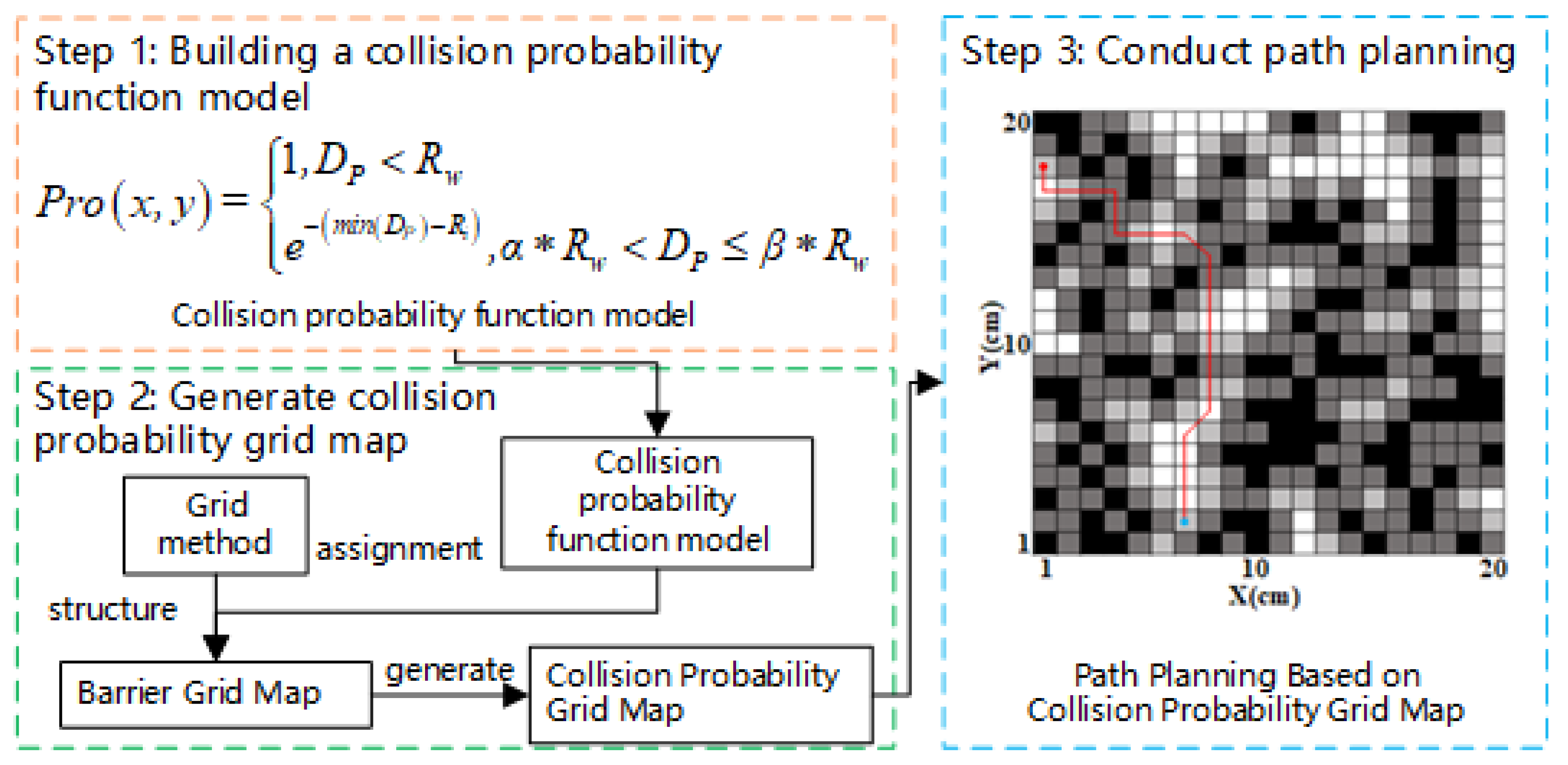
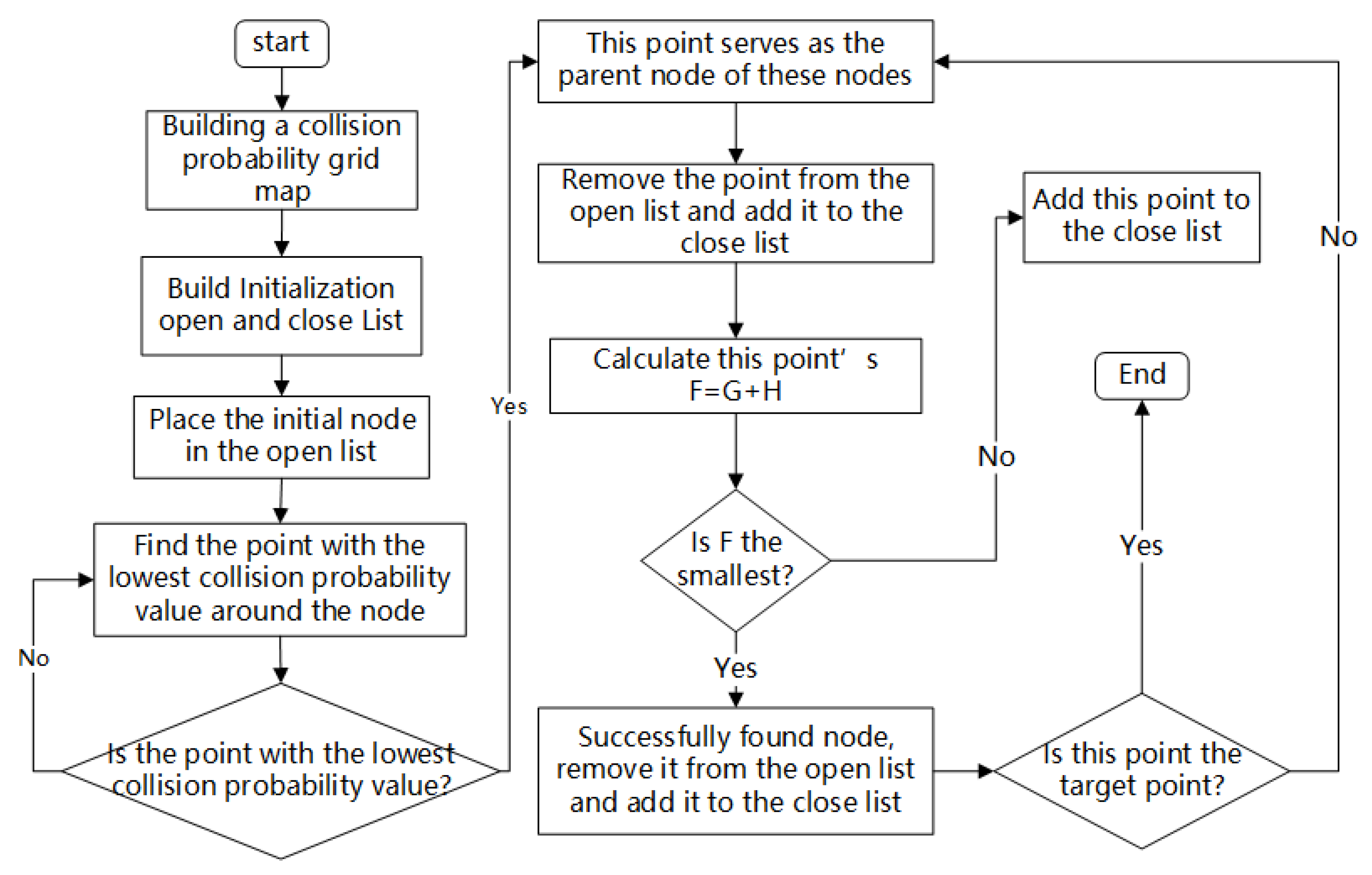
The goal of this article is to construct an environmental map with collision probability information and conduct path planning based on this in order to plan a path with high security. Therefore, we have designed a map construction and path planning method based on collision probability models. Figure 1 provides an overview of the process of planning a secure path using the method presented in this article.
This method is divided into three steps. (1) Construct a collision probability function model that considers the size of the robot and the distance between the robot and the obstacle. (2) Based on the grid method, an obstacle grid map is constructed, and on this basis, a collision probability function model is used to assign values to idle grids, ultimately forming a CPGM. (3) Based on the CPGM, the traditional A* algorithm is improved by utilizing the collision probability information in the map, and a safe and optimal navigation path for mobile robots is planned.
3.1. Collision Probability Function Model
In general path planning problems, mobile robots are often viewed as a particle. Although the optimal running path is obtained, the size of the mobile robot itself and the probability of collision with obstacles are not considered, making it easy for mobile robots to collide with obstacles. We consider analyzing the collision probability of mobile robots in the path planning process based on the size of the robot itself and the probability of collision between the robot and obstacles.
3.1.1. Definition of Collision Probability
The collision situations of robots during autonomous navigation can be divided into three states: fatal, dangerous, and safe [31], and the occurrence of these three states can be described by collision probability. The collision probability is the probability of a collision occurring between the center of the grid occupied by the mobile robot and the center of the obstacle. The grids in the grid map that are not occupied by obstacles are represented as 0, while the grids occupied by obstacles are represented as 1 [32]. Therefore, the range of collision probability values in this article is also represented as 0–1.
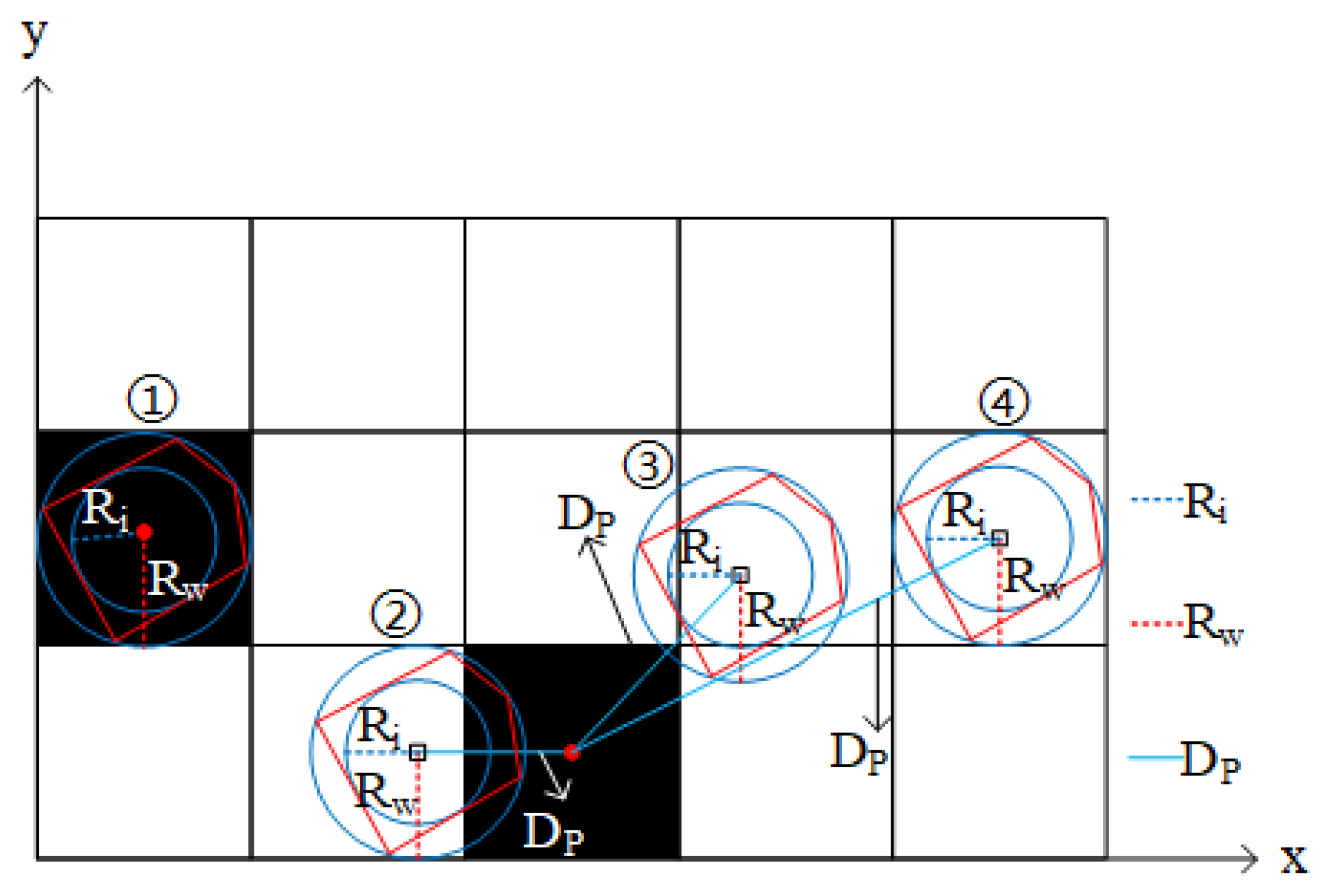
Assuming the edge length of each grid in a grid map is , the inscribed radius of the contour projected by the mobile robot on the ground is , the radius of the circumscribed circle is , and the distance between the center of the robot occupying the grid and the center of the obstacle grid is , as shown in Figure 2, which shows the position relationship between a mobile robot and obstacles while driving in a grid map.
From Figure 2, collision probability between the robots and obstacles can be divided into the following two situations:
- (1)
- When the distance between the center of the robot occupying the grid and the center of the obstacle grid is less than the radius of the robot’s inscribed circle, that is, , at this point the obstacle overlaps with the center of the robot, as shown in the first scenario in Figure 2. When the center of the robot occupies a distance between the grid and the center of the obstacle grid that is greater than the grid edge length and less than the radius of the robot’s outer circle, that is, , at this point the obstacle is within the inscribed circle of the robot, as shown in the second case in Figure 2, and is bound to collide. When the distance between the center of the robot occupying the grid and the center of the obstacle grid is greater than the radius of the inscribed circle and less than the radius of the robot’s circumscribed circle, that is, , at this point, the obstacle is located within the outer tangent circle of its robot, as shown in the third scenario in Figure 2. It is at the collision threshold and may not necessarily collide, but it is very dangerous. Therefore, the above three situations are all marked as fatal zones, with a collision probability value range of 1. The specific calculation method is shown in Formula (1).
In Equation (1), is the collision probability of grid .
- (2)
- When the distance between the center of the robot occupying the grid and the center of the obstacle grid is greater than the radius of the robot’s circumscribed circle, that is, , at this point, the collision between the robot and the obstacle is caused by and , the value of which is determined, as shown in the fourth case in Figure 2, which is only an example of a collision situation. If and have a smaller value, and if it is closer to the obstacle, then it is recorded as a danger zone; If and have a larger value, and if it is farther away from the obstacle, then it is denoted as a safety zone, and the range of collision probability values for its grid is , the farther away from the obstacle, the lower the probability of collision. The specific calculation method is shown in Formula (2).
In Equation (2), is a collision probability exponential descent function constructed using the minimum Euclidean distance between the center of the grid occupied by the robot and the center of the obstacle grid; is the minimum distance set from the center of the grid occupied by the robot to the center of the obstacle grid.
The calculation method for the distance between the center of the robot occupying the grid and the center of the obstacle grid is shown in Formula (3).
In Equation (3), is the grid coordinate of the obstacle center grid; is the grid coordinate where the robot occupies the center of the grid.
3.1.2. Expression of Collision Probability Function
After the detailed analysis and derivation in the above summary, the collision probability function model in this article can be summarized as Formula (4).
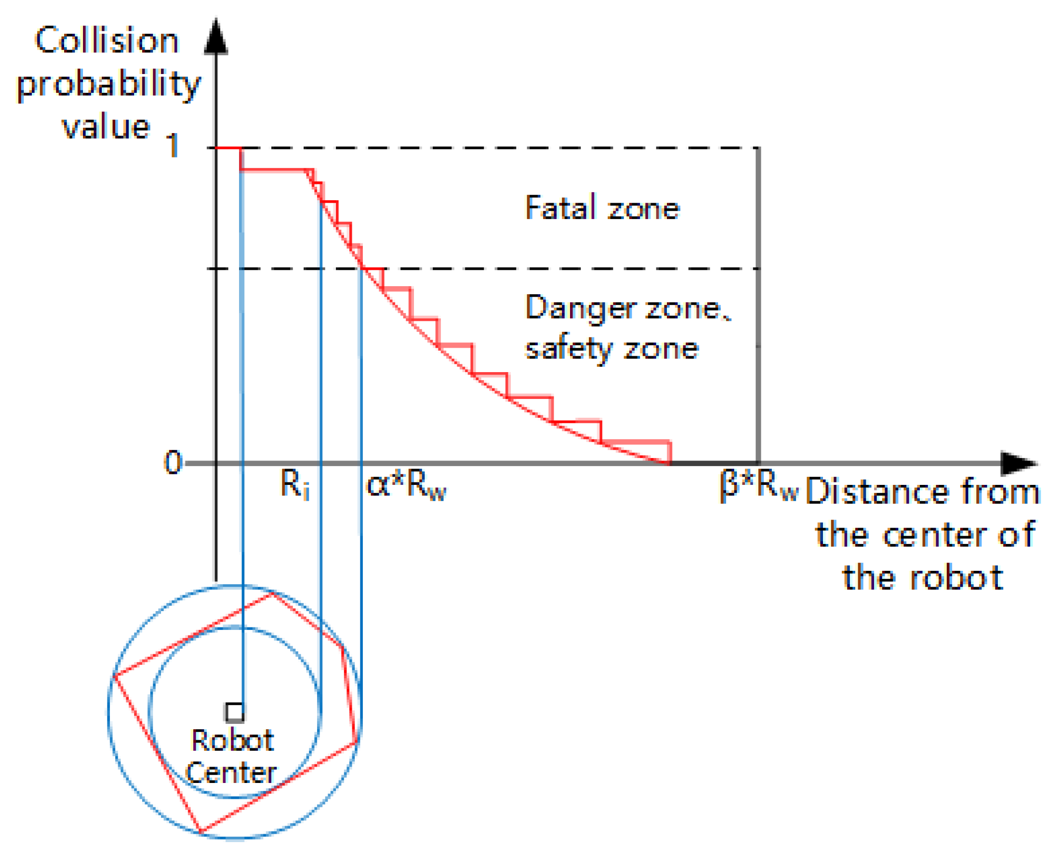
According to the collision probability function model, the probability of collision between robots and obstacles can be summarized as shown in Figure 3.
3.2. Construction of Collision Probability Grid Map
Establishing an environmental map is a prerequisite for path planning. This article constructs an obstacle grid map containing obstacle information based on the grid method and uses the collision probability values in the collision probability function model to fill the grids around the obstacles based on the obstacle grid map so that these grids have collision probability information, thus obtaining a CPGM. This solves the problem of the simple structure of traditional grid methods in building navigation maps and the issue of lack of security information.
3.2.1. Construction of Obstacle Grid Map
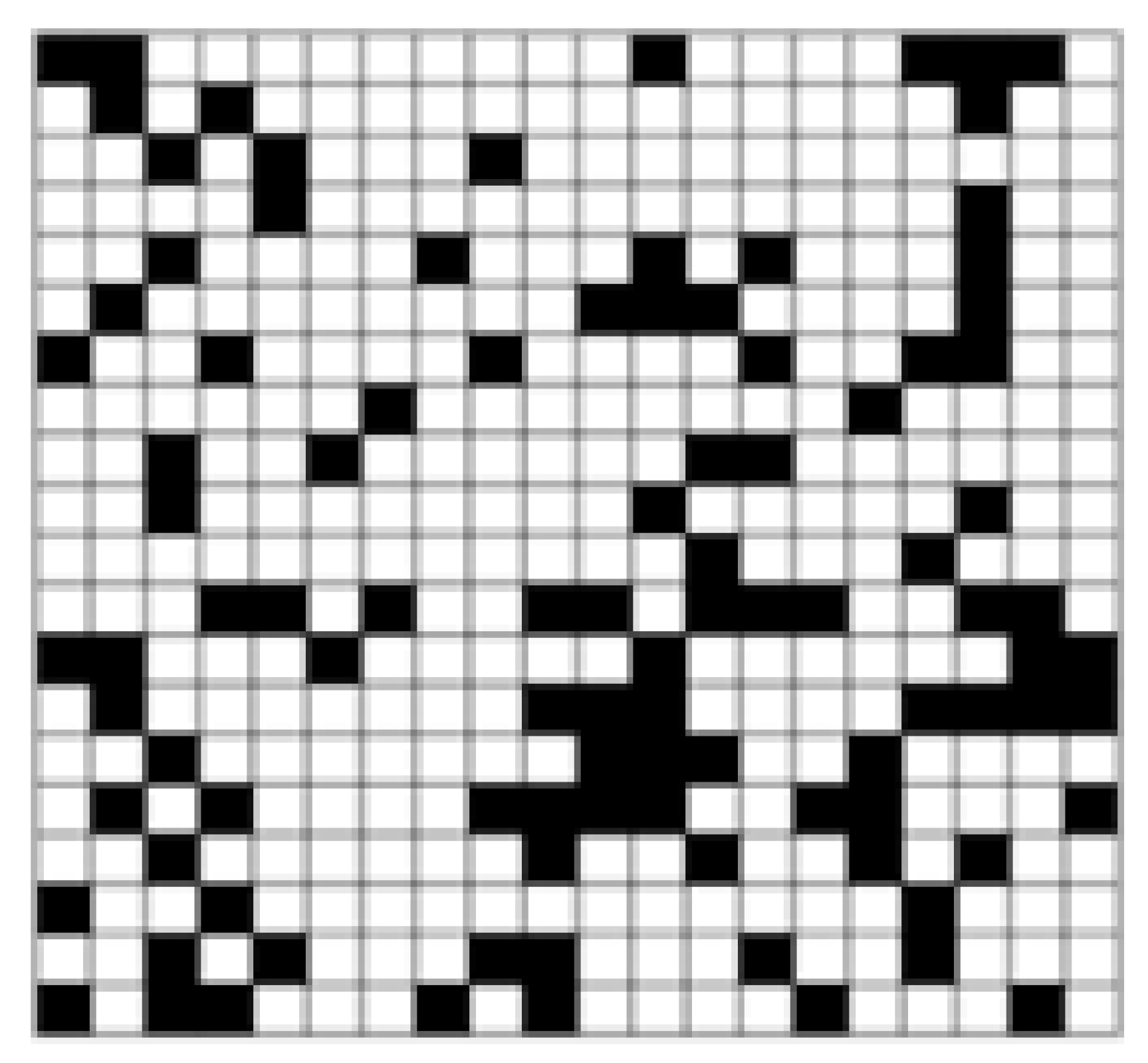
The process of converting an environmental model into a grid map mainly involves dividing the environment into small square areas, called grids. Each grid represents a part of the environment, and each grid is associated with the storage of environmental attributes such as color, height, obstacles, etc. [33]. As shown in Figure 4, the environmental information is simplified into two color grids, where the white grids represent the navigable area of the robot, the black grids represent the non-navigable area (obstacle area), and obstacles that do not occupy the complete grid are inflated. Transforming the key environmental information into raster data can facilitate computer analysis and operation, and improve the robot’s ability to perceive the environment. Therefore, this article uses the grid method to generate a grid map of obstacles of size in MATLAB.
3.2.2. Construction of CPGM
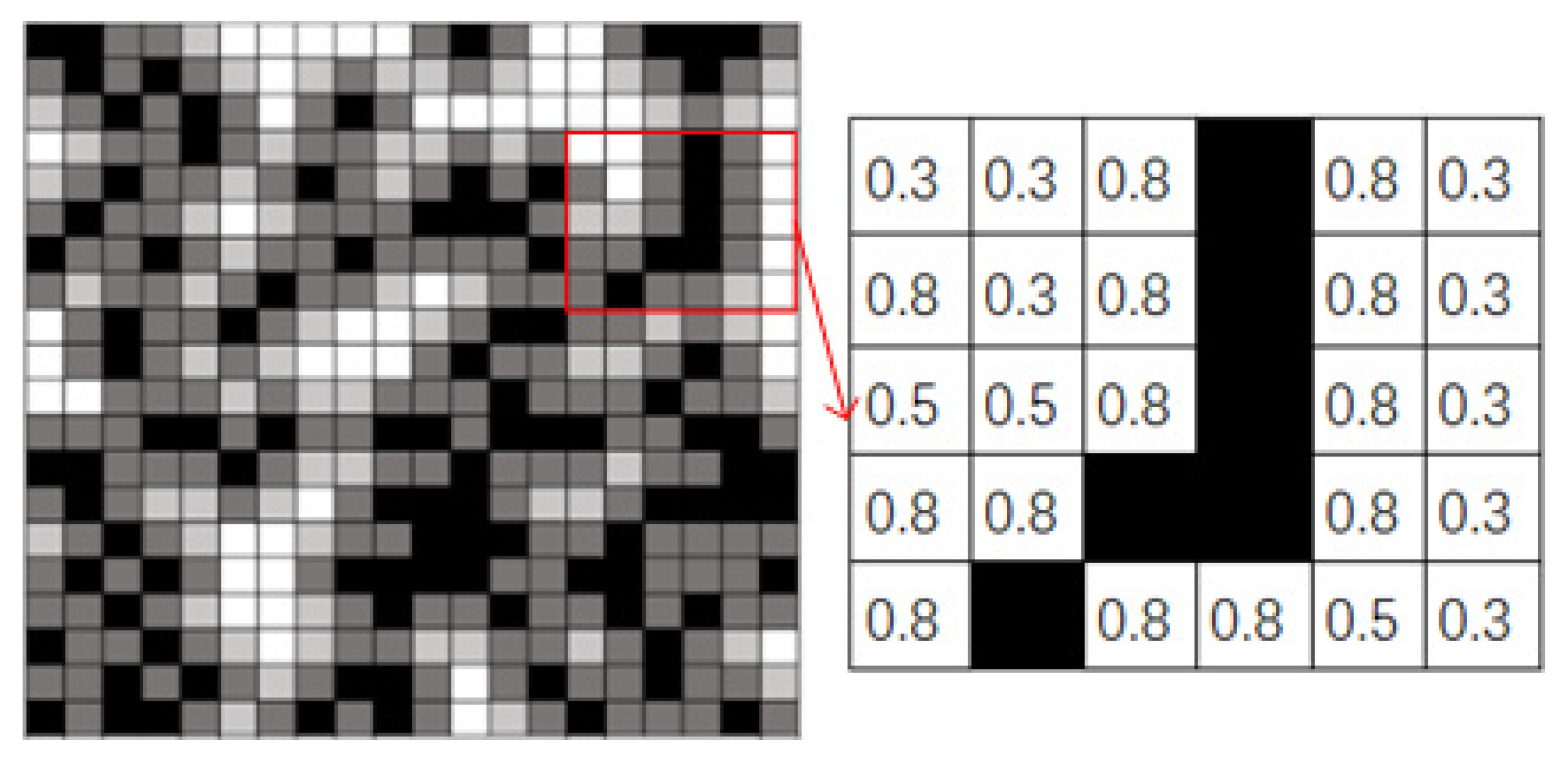
Based on the collision probability function model, we assign collision probability values to the idle grids in the obstacle grid map except for obstacles, in order to obtain a grid map containing collision probability information, so that the robot can avoid obstacles to the maximum extent during subsequent path planning. The CPGM constructed is shown in Figure 5.
In Figure 5, if the distance between the center of the robot occupying the grid and the center of the obstacle grid is less than or equal to the radius of the robot’s circumscribed circle, the collision probability value of the idle grid is assigned a value of 1, which is a black grid representing the non-navigable area. If the distance between the center of the robot occupying the grid and the center of the obstacle grid is greater than the radius of the robot’s circumscribed circle, the idle grid is assigned a value based on the collision probability index descent function , namely gray and white grids, representing the navigable area. Among them, the gray grid represents the hazardous area, and the collision probability value of the gray grid is assigned as 0.8 or 0.5. The farther away from the obstacle, the lower the collision probability value, and the color gradually becomes lighter. The white grid represents the safe area, and the collision probability value of the white grid is assigned a value of 0.3.
3.3. Path Planning Based on CPGM
3.3.1. Traditional A* Algorithm
The A* algorithm is a path planning algorithm proposed by Hart. Its basic idea is to use a heuristic search and Dijkstra algorithm to find the shortest path from the initial point to the target point. During the search process, the A* algorithm maintains two values: the actual cost function from the initial point to the current node, and the heuristic function from the current node to the target point. The calculation of the total cost of the current node allows for the evaluation of the priority of the node and prioritization of the expanding of the node with the lowest cost until the target point is found or expansion cannot continue. This can minimize the number of searches and quickly locate the target point while ensuring the shortest path is found. The total cost of the classic A* algorithm is shown in Formula (5).
In Equation (5): represents the total cost of searching from the initial node S to the target node E; represents the actual cost function of the robot from the initial node S to the current node N; is a heuristic function used to estimate the distance from the current node N to the target node E.
3.3.2. Improved A* Algorithm
In the node traversal process of the traditional A* algorithm, regardless of how far the node is from the obstacle, the cost incurred by the robot through it is considered equal. However, in practice, the distance between the obstacle and the robot is not equivalent to the collision state of the robot, but is inversely proportional to the distance between them. Therefore, based on the CPGM, we integrate the collision probability values in the map into the actual cost function for calculation, and the definition expression is shown in Formula (6).
In Equation (6): is the distance cost of the robot in the path; is the collision probability value of the robot at the end node of the path segment; and represent the weighting coefficient, and using , by adjusting the weights, paths that meet different requirements can be obtained.
The quality of the heuristic function will directly affect the path planned by the A* algorithm, and the Euclidean distance is generally used to construct the heuristic function. However, when planning the path of mobile robots, they will be affected by complex obstacles and add new turning points, which will affect the results of path planning. In order to reduce turning points while ensuring the planning of the shortest path, the heuristic function defined in this article is shown in Formula (7).
In Equation (7): is the transfer weight coefficient, which can be adjusted to change the impact of the estimated cost on path planning, and are the coordinates of the current node N and the target node E.
3.3.3. The Specific Process of the Improved A* Algorithm
In the classic A* algorithm, the travel mode of the path follows the eight-domain travel mode. The advantage of this mode is that it can display the advantages and disadvantages of the algorithm in a concise and visual manner, but it ignores the safety of the path. Therefore, the algorithm in this article integrates the collision probability value into the actual cost function based on the CPGM, resulting in higher path safety. The process is shown in Figure 6.
4. Experiment and Analysis
This article establishes a simulation environment in MATLAB, conducts CPGM construction experiments under the same obstacle distribution, and compares the algorithm proposed in this article with traditional A*, the algorithm presented in reference [37], and the algorithm presented in reference [38], verifying the feasibility and effectiveness of the proposed method.
4.1. Experiment and Analysis of Constructing the CPGM
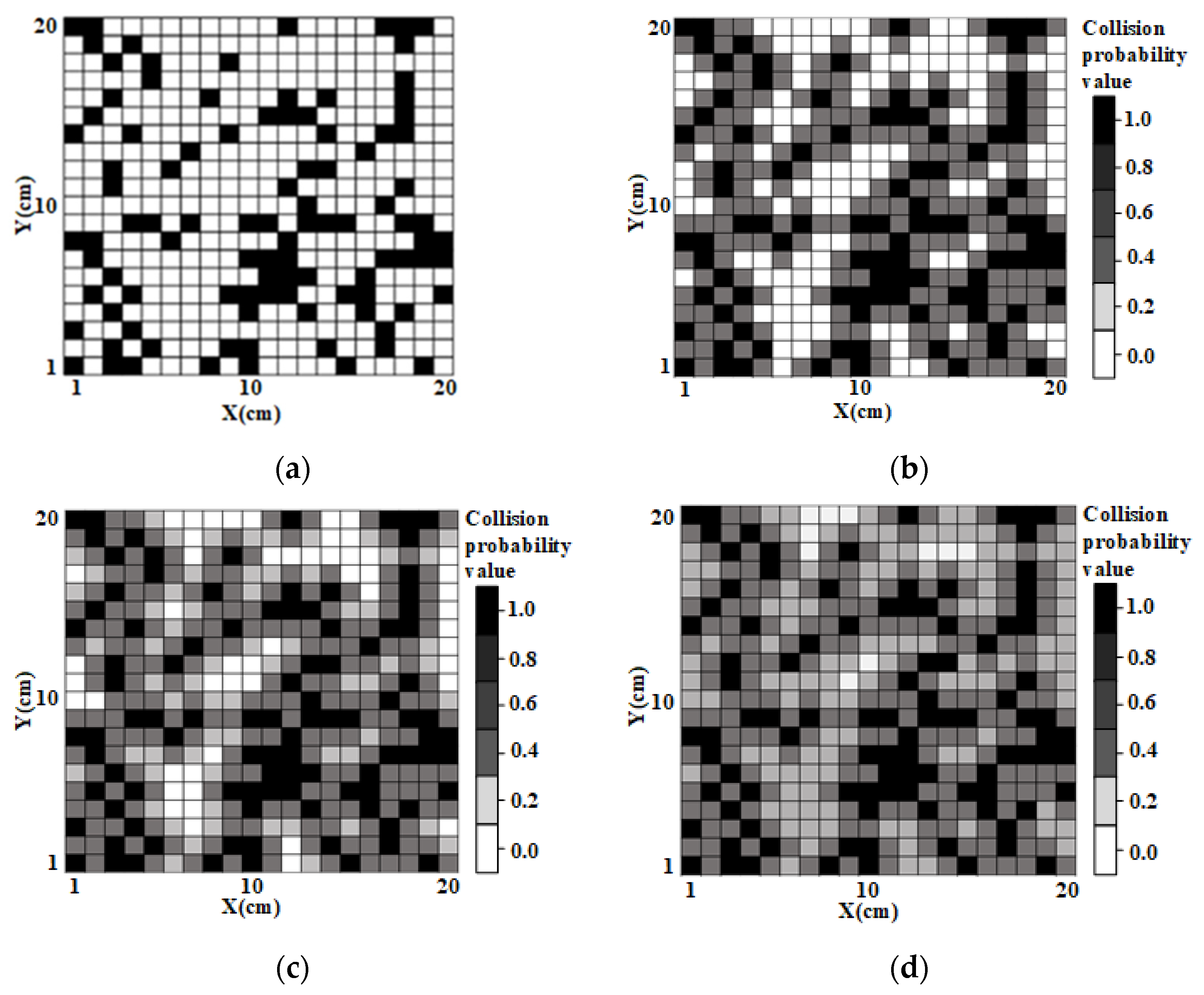
In the experiment, a size grid map was established in MATLAB as the working environment of the mobile robot. The grid edge length of the working environment of the mobile robot was set as 1 cm, and the original grid map is shown in Figure 7a. Randomly change the position of the robot and conduct multiple repeated experiments according to the different collision state division rules. Each group of experiments judges the rationality of the division based on the collision probability value.
Comparative experiments were conducted by changing the range of different collision states to obtain different CPGMs, as shown in Figure 7b–d. In Figure 7, “Collision State 1” divides into a fatal zone, into a dangerous zone, and into a free zone; “Collision State 2” divides into a fatal zone, into a dangerous zone, and into a free zone; “Collision State 3” divides into a fatal zone, into a dangerous zone, and into a free zone. Among them, the black part represents the location of the obstacle and is the fatal zone in the collision state, and the gray part represents the danger zone in the collision state, which is divided according to different collision states. The darker the color, the more dangerous it is. The white part represents the free zone in the collision state.
From the colors in Figure 7, it can be seen that in “Collision State 1”, the fatal and dangerous areas are too close to the obstacle, which can easily cause the planned path to stick closely to the obstacle. Compared with “Collision State 1”, “Collision State 2” doubles the scope of the danger zone outward, and the planned path is safer and less prone to collision with obstacles. Compared to “Collision State 2”, “Collision State 3” may double the scope of the danger zone and reduce the probability of robot collision with obstacles, but it may result in the planned path not being efficient enough. Therefore, this article chooses , as the hazardous area and , as the free zone.
4.2. Experiment and Analysis of Path Planning Based on CPGM
In order to verify the effectiveness of the algorithm proposed in this paper, many computer simulations were conducted by setting multiple sets of different parameters. The experimental environment is Windows 10, Intel Core i7, with 8 GB of memory, and the compilation environment is MATLAB 2020 (b).
4.2.1. Simulation of Different Parameters
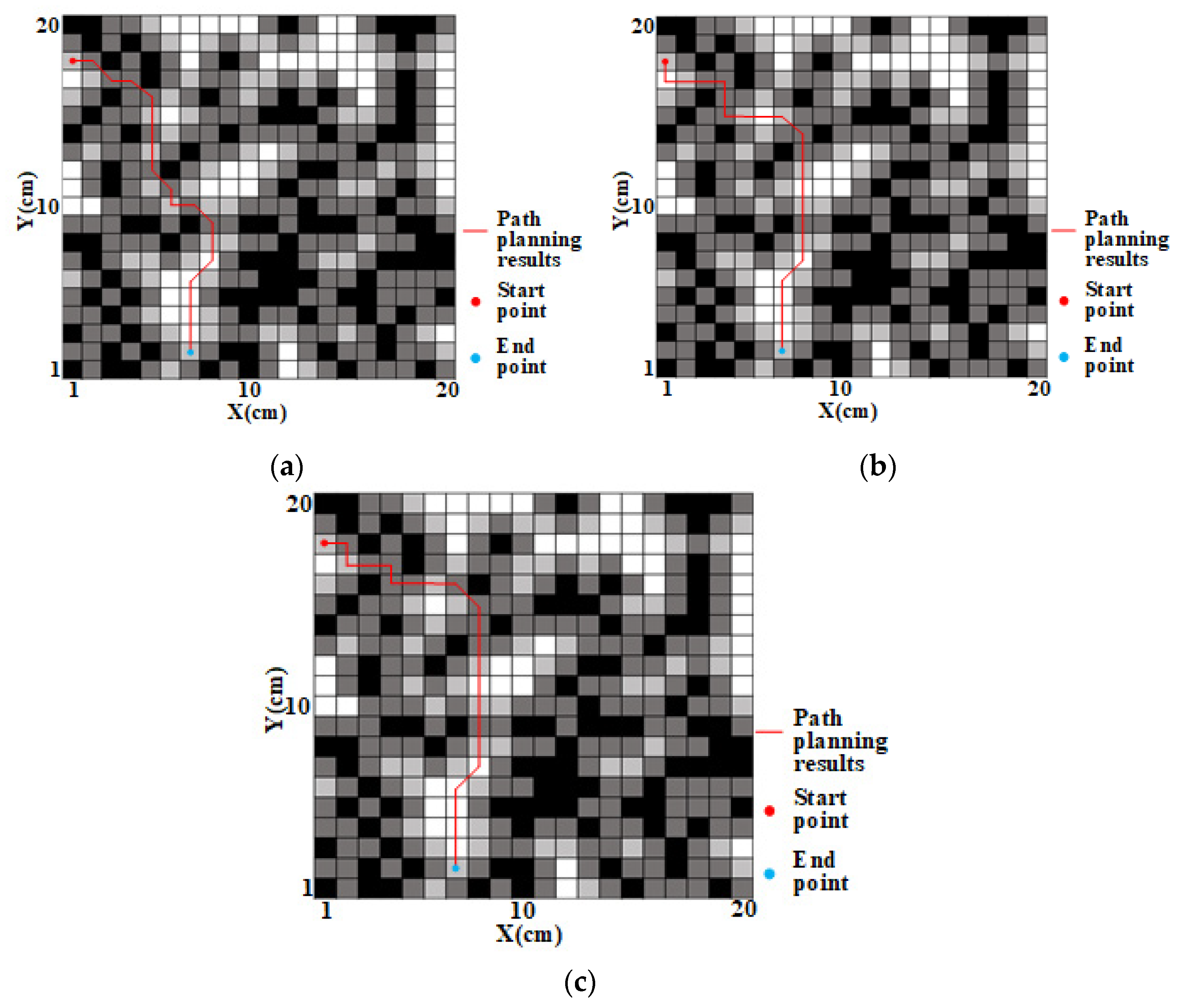
To investigate the impact of the different weighting coefficients and on the proposed algorithm, take the collision probability value in the fatal zone, the collision probability value in the dangerous zone, and the collision probability value in the free zone. Then take different and for multiple sets of simulations. The results are shown in Figure 8a–c.
As shown in Figure 8, in the CPGM, red represents the starting point and blue represents the ending point. Taking different and for simulation can obtain path planning diagrams with different effects. The specific data are shown in Table 1.
From Table 1, compared to the traditional A* algorithm, the algorithm in this article can plan a more optimal path when selecting different weighting coefficients. When the value of is fixed, if the value of is larger and the value of is smaller, the proportion of distance cost is larger and the proportion of collision probability is smaller. At this point, the longer the path length, the longer the algorithm time, and the lower the proportion of dangerous nodes, that is, the safer the path and the farther away from obstacles. Although the new path is smoother, its number of turns varies irregularly. From Table 1, when , is used, the length and algorithm time obtained from path planning increase compared to when , is used, but decrease compared to when , is used, and the proportion of dangerous nodes is not significantly different from when , is used with fewer turns. Therefore, this article takes the weighting coefficient as , .
4.2.2. Simulation of Different Algorithms
By conducting simulation experiments on the traditional A* algorithm, the algorithm in reference [37], the presented in reference [38], and our algorithm in CPGM scenarios, this paper tests the effectiveness of the proposed algorithm by analyzing different algorithms in path planning length, algorithm time, proportion of dangerous nodes, and number of turns. The simulation results of different algorithms in path planning are shown in Figure 9a–d, and their simulation data are shown in Table 2.
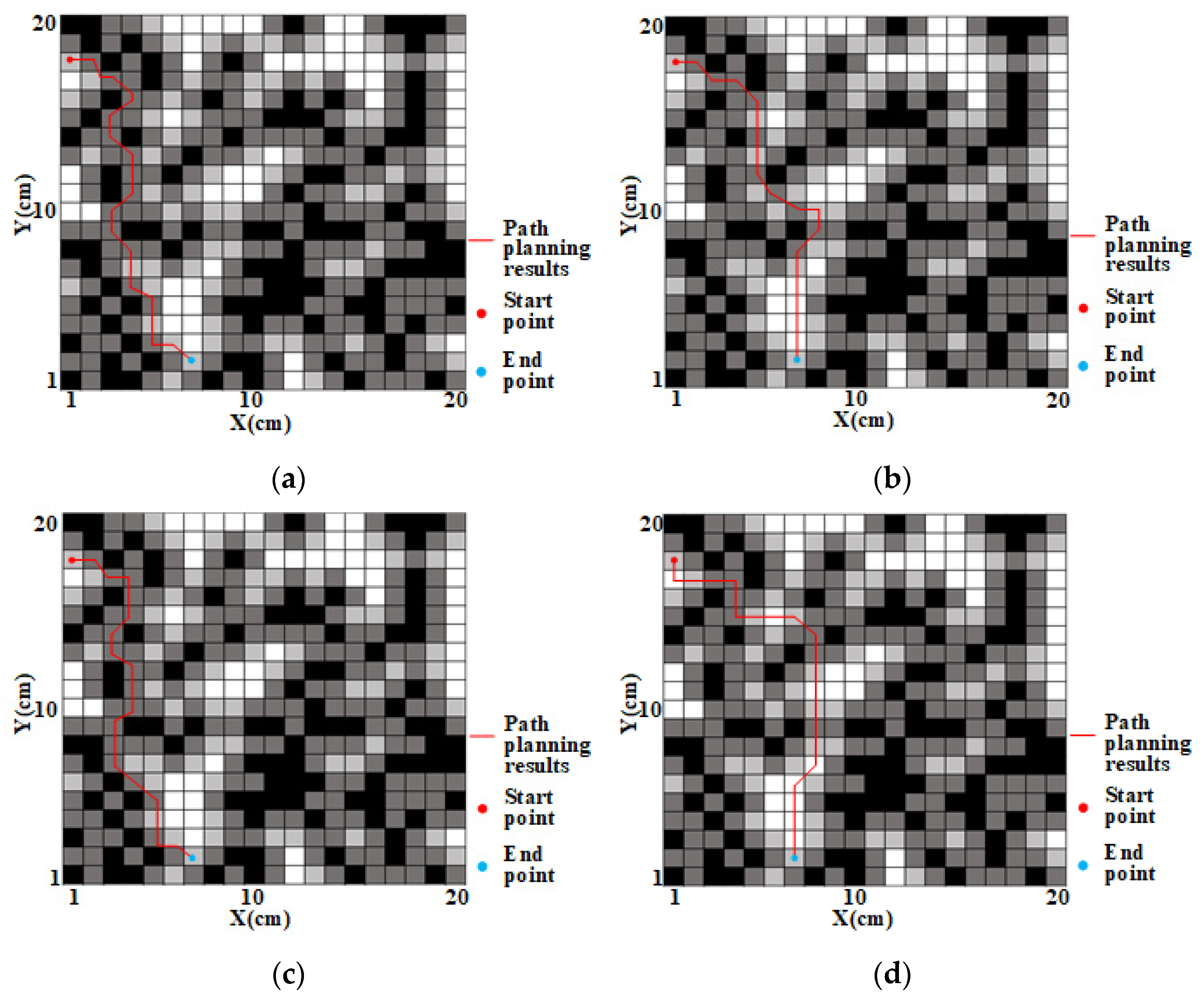
From Table 2 and Figure 9, it can be seen that the traditional A* algorithms plan paths with multiple inflection points that are close to the edges and endpoints of obstacles. Compared with the traditional A* algorithm, the algorithm in reference [37] shows that the planned path is relatively smooth and not close to the edge of the obstacle, but it does not solve the problem of the planned path being close to the endpoint of the obstacle. Compared with the traditional A* algorithm, the algorithm in reference [38] has a slightly smoother planned path, but it does not solve the problem of the planned path being close to the edges and endpoints of the obstacles. The paths planned by these three algorithms are prone to collisions between robots and obstacles, and the paths are not smooth enough. The path planned by the method in this article is not only smoother and reduces inflection points but also has a certain safe distance from obstacles, resulting in higher safety of the robot during driving.
4.2.3. Simulation of Different Obstacle Ratios
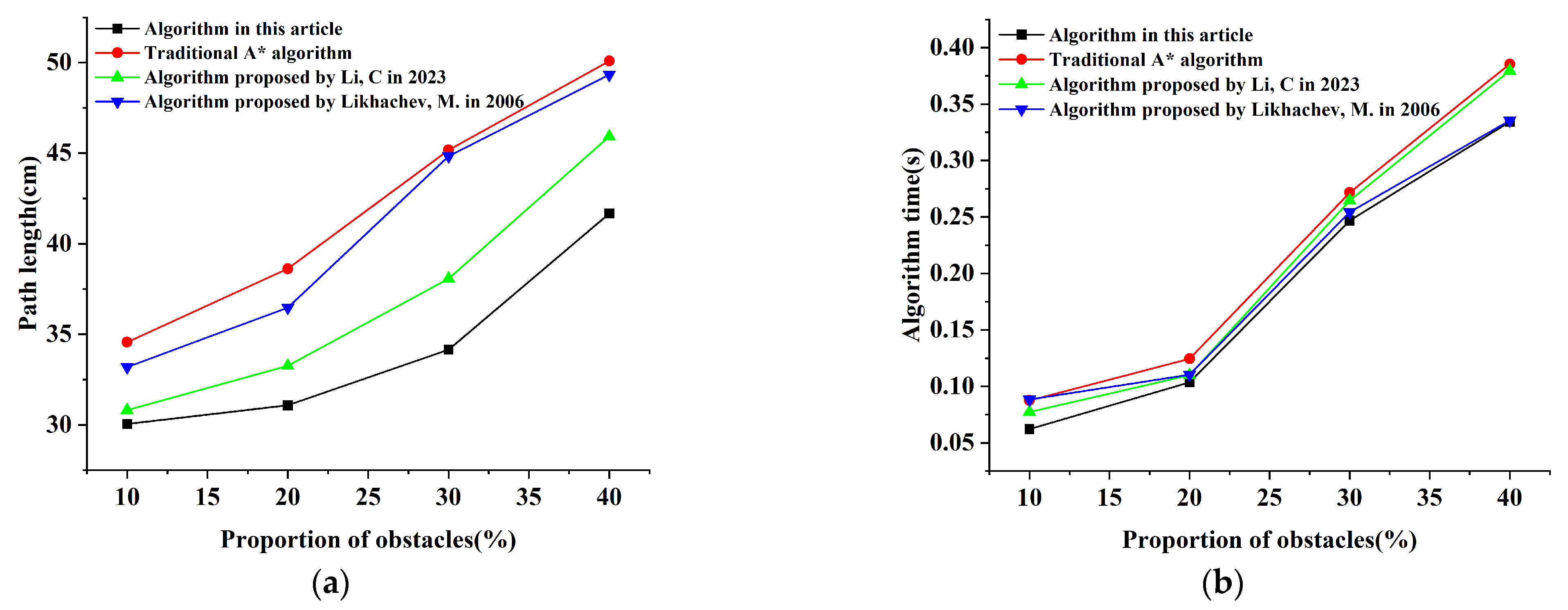
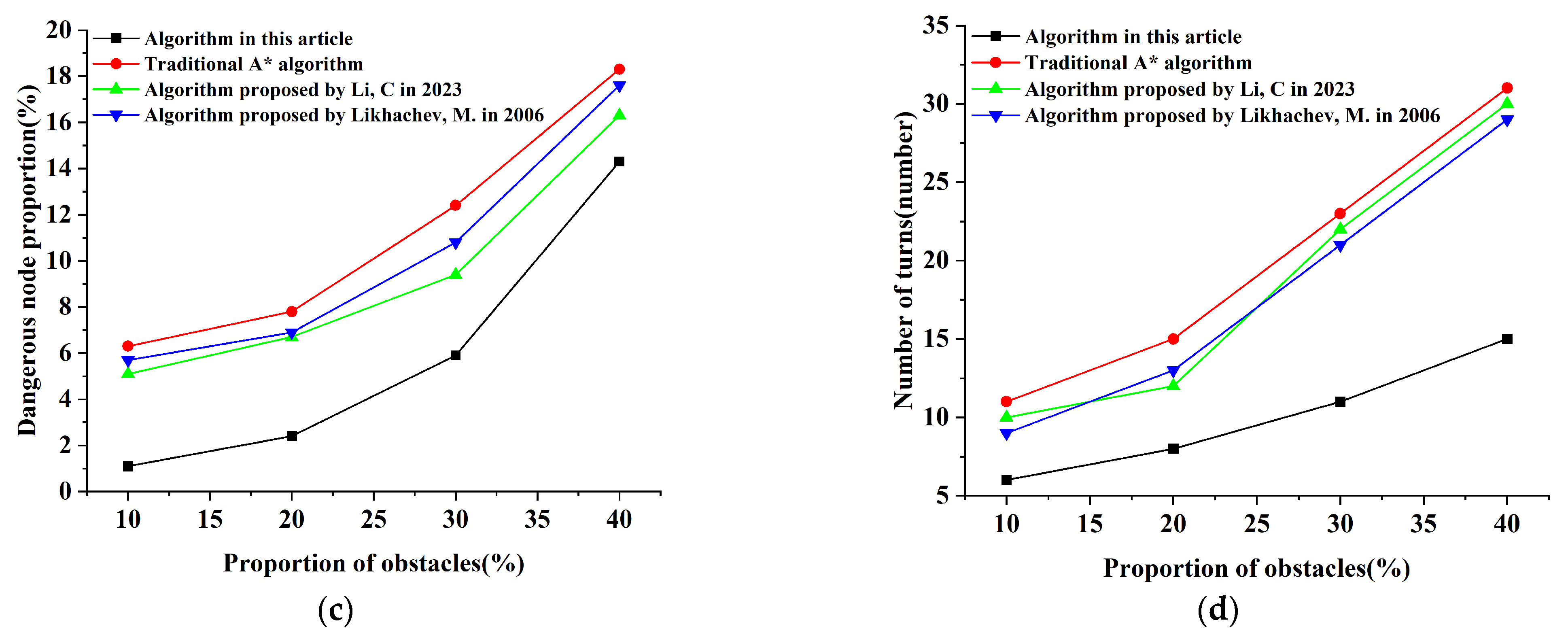
By establishing a collision probability grid map of size , randomly generate obstacle nodes of different proportions, obtain different obstacle environment models, and specify that no obstacles are generated at the starting and ending points. Four cases of obstacle ratio p = 10%, p = 20%, p = 30%, and p = 40% were selected for experiments. Each group randomly generated 10 different models, and then used the traditional A* algorithm, the algorithm in reference [37], the algorithm in reference [38], and this article’s algorithm to independently operate in different environmental models. The average values of each parameter of the obtained path in each group were compared, and the collision probability value in the fatal zone and the collision probability value in the dangerous zone were specified, the collision probability value and parameter , of the free zone remained unchanged. The simulation results are shown in Figure 10a–d.
Figure 10 shows the comparison of various parameters for path planning using four algorithms under different obstacle ratios. The specific data are shown in Table 3.
From Table 3, compared with the traditional A* algorithm, the algorithm in reference [37], and the algorithm in reference [38], the path length, algorithm time, proportion of dangerous nodes, and number of turns planned by the algorithm in this paper have all decreased. And from Figure 10, the higher the proportion of obstacles, the more complex the map is, and the search time of all four algorithms has increases. However, compared to the other three algorithms, the search time used in this algorithm is significantly reduced. Through analysis, the algorithm proposed in this article can significantly improve the efficiency of path planning, effectively reduce the number of path nodes, and reduce path costs. Compared to the traditional A* and algorithm in reference [37], the algorithm in reference [38] can more easily find a collision free feasible path.
5. Conclusions
In this article, we propose a map construction and path planning method based on collision probability models. Through this method, we can find a safer, more efficient and optimal path in complex environments. This study solves the problems of simple structure, lack of collision probability information, and planning an optimal anti-collision safety path in the navigation grid map constructed by using traditional grid methods. By comparing various algorithms through extensive simulation experiments in MATLAB, the following conclusions can be drawn:
- (1)
- By setting different parameters for the radius of the outer circle between the robot and the obstacle, we obtained a reasonable range for dividing the danger zone and safety zone between the robot and the obstacle and constructed a CPGM. Compared with other grid map construction methods, this map contains collision probability information, which improves the safety for subsequent path planning.
- (2)
- The path planned by the method used in this study will not be close to the edge or endpoint of the obstacle, and the length of the planned path will be shorter than the other three algorithms, with less search time and smoother paths, greatly improving the safety of the paths planned by the algorithm. This is because we add collision probability values into the actual cost function of the traditional A* algorithm, so that every time we search for the node with the lowest cost, the collision probability is also minimized.
However, our algorithm still has some limitations. Therefore, we will make the following improvements in our future work:
- (1)
- Our method is only applicable to static mobile robot navigation scenarios and cannot avoid dynamic obstacles. Therefore, how to plan a safer, more efficient, and more path-optimized path in dynamic and complex obstacle environments will be the focus of our next research.
- (2)
- Our method still needs to be improved in terms of running speed. We will improve the running speed of our algorithm in the future by ensuring that we can plan more secure paths.
Author Contributions
Conceptualization, J.L. and W.T.; methodology, J.L.; software, Y.L.; validation, J.L., J.J. and D.Z.; formal analysis, W.T.; investigation, D.F.; resources, J.J.; data curation, J.J.; writing—original draft preparation, W.T.; writing—review and editing, J.L.; visualization, J.J.; supervision, J.J.; project administration, W.T.; funding acquisition, J.J. All authors have read and agreed to the published version of the manuscript.
Funding
This research was funded by the National Natural Science Foundation of China, (No. 41961063); Guilin City Technology Application and Promotion Project in 2022 (20220138-2); Key R&D Projects in Guilin City in 2022 (20220109).
Data Availability Statement
Not applicable.
Conflicts of Interest
The authors declare no conflict of interest.
References
- Buniyamin, N. Ant colony system for robot path planning in global static environment. In Proceedings of the 9th WSEAS International Conference on System Science and Simulation in Engineering, Stevens Point, WI, USA, 4–6 October 2010; pp. 192–197. [Google Scholar]
- Chunhui, Z.; Green, R. Vision-based autonomous navigation in indoor environments. In Proceedings of the 25th International Conference of Image and Vision Computing New Zealand, Queenstown, New Zealand, 8–9 November 2010; pp. 1–7. [Google Scholar] [CrossRef]
- Sariff, N.; Buniyamin, N. An Overview of Autonomous Mobile Robot Path Planning Algorithms. In Proceedings of the 2006 4th Student Conference on Research and Development, Shah Alam, Malaysia, 27–28 June 2006; pp. 183–188. [Google Scholar] [CrossRef]
- Li, Y.; Ma, S. Navigation of Apple Tree Pruning Robot Based on Improved RRT-Connect Algorithm. Agriculture 2023, 13, 1495. [Google Scholar] [CrossRef]
- Mac, T.T.; Copot, C.; Tran, D.T.; De Keyser, R. Heuristic approaches in robot path planning: A survey. Robot. Auton. Syst. 2016, 86, 13–28. [Google Scholar] [CrossRef]
- Thrun, S. Learning metric-topological maps for indoor mobile robot navigation. Artif. Intell. 1998, 99, 21–71. [Google Scholar] [CrossRef]
- Guivant, J.; Nebot, E.; Nieto, J.; Masson, F. Navigation and mapping in large unstructured environments. Int. J. Robot. Res. 2004, 23, 449–472. [Google Scholar] [CrossRef]
- Lau, B.; Sprunk, C.; Burgard, W. Efficient grid-based spatial representations for robot navigation in dynamic environments. Robot. Auton. Syst. 2013, 61, 1116–1130. [Google Scholar] [CrossRef]
- Wang, K.; Xu, J.; Song, K.; Yan, Y.; Peng, Y. Informed anytime Bi-directional Fast Marching Tree for optimal motion planning in complex cluttered environments. Expert Syst. Appl. 2023, 215, 119263. [Google Scholar] [CrossRef]
- Dijkstra, E.W. A Note on Two Problems in Connexion with Graphs. In Edsger Wybe Dijkstra: His Life, Work, and Legacy; Association for Computing Machinery: New York, NY, USA, 2022; Volume 45, pp. 287–290. [Google Scholar] [CrossRef]
- Hart, P.E.; Nilsson, N.J.; Raphael, B. A Formal Basis for the Heuristic Determination of Minimum Cost Paths. IEEE Trans. Syst. Sci. Cybern. 1968, 4, 100–107. [Google Scholar] [CrossRef]
- Bozek, P.; Karavaev, Y.L.; Ardentov, A.A.; Yefremov, K.S. Neural network control of a wheeled mobile robot based on optimal trajectories. Int. J. Adv. Robot. Syst. 2020, 17, 1729881420916077. [Google Scholar] [CrossRef]
- Liu, X.; Wang, W.; Li, X.; Liu, F.; He, Z.; Yao, Y.; Ruan, H.; Zhang, T. MPC-based high-speed trajectory tracking for 4WIS robot. ISA Trans. 2022, 123, 413–424. [Google Scholar] [CrossRef]
- Zahid, T.; Kausar, Z.; Shah, M.F.; Saeed, M.T.; Pan, J. An Intelligent Hybrid Control to Enhance Applicability of Mobile Robots in Cluttered Environments. IEEE Access 2021, 9, 50151–50162. [Google Scholar] [CrossRef]
- Alireza, M.; Vincent, D.; Tony, W. Experimental study of path planning problem using EMCOA for a holonomic mobile robot. J. Syst. Eng. Electron. 2021, 32, 1450–1462. [Google Scholar] [CrossRef]
- Ali, H.; Gong, D.; Wang, M.; Dai, X. Path planning of mobile robot with improved ant colony algorithm and MDP to produce smooth trajectory in grid-based environment. Front. Neurorobotics 2020, 14, 44. [Google Scholar] [CrossRef] [PubMed]
- Tang, G.; Tang, C.; Claramunt, C.; Hu, X.; Zhou, P. Geometric A-Star Algorithm: An Improved A-Star Algorithm for AGV Path Planning in a Port Environment. IEEE Access 2021, 9, 59196–59210. [Google Scholar] [CrossRef]
- Zheng, T.; Xu, Y.; Zheng, D. AGV Path Planning based on Improved A-star Algorithm. In Proceedings of the 2019 IEEE 3rd Advanced Information Management, Communicates, Electronic and Automation Control Conference (IMCEC), Chongqing, China, 11–13 October 2019; pp. 1534–1538. [Google Scholar] [CrossRef]
- Erke, S.; Bin, D.; Yiming, N.; Qi, Z.; Liang, X.; Dawei, Z. An improved A-Star based path planning algorithm for autonomous land vehicles. Int. J. Adv. Robot. Syst. 2020, 17, 1729881420962263. [Google Scholar] [CrossRef]
- Zhang, Z.; Wan, Y.; Wang, Y.; Guan, X.; Ren, W.; Li, G. Improved hybrid A* path planning method for spherical mobile robot based on pendulum. Int. J. Adv. Robot. Syst. 2021, 18, 1729881421992958. [Google Scholar] [CrossRef]
- Ge, H.; Ying, Z.; Chen, Z.; Zu, W.; Liu, C.; Jin, Y. Improved A* Algorithm for Path Planning of Spherical Robot Considering Energy Consumption. Sensors 2023, 23, 7115. [Google Scholar] [CrossRef] [PubMed]
- Huang, B.; Wu, Q.; Zhan, F.B. A shortest path algorithm with novel heuristics for dynamic transportation networks. Int. J. Geogr. Inf. Sci. 2007, 21, 625–644. [Google Scholar] [CrossRef]
- Martins, O.O.; Adekunle, A.A.; Olaniyan, O.M.; Bolaji, B.O. An Improved multi-objective a-star algorithm for path planning in a large workspace: Design, Implementation, and Evaluation. Sci. Afr. 2022, 15, e01068. [Google Scholar] [CrossRef]
- Hong, Y.; Kim, S.; Kim, Y.; Cha, J. Quadrotor path planning using A* search algorithm and minimum snap trajectory generation. ETRI J. 2021, 43, 1013–1023. [Google Scholar] [CrossRef]
- Lima, J.; Costa, P.; Costa, P.; Eckert, L.; Piardi, L.; Moreira, A.P.; Nakano, A. A* search algorithm optimization path planning in mobile robots scenarios. AIP Conf. Proc. 2019, 2116, 220005. [Google Scholar] [CrossRef]
- Yue, G.; Zhang, M.; Shen, C.; Guan, X. Bi-directional smooth A-star algorithm for navigation planning of mobile robots. Sci. Sin. Technol. 2021, 51, 459–468. [Google Scholar] [CrossRef]
- Hui, Q.; Cheng, J. Motion planning for AmigoBot with line-segment-based map and Voronoi diagram. In Proceedings of the 2016 Annual IEEE Systems Conference (SysCon), Orlando, FL, USA, 18–21 April 2016; pp. 1–8. [Google Scholar] [CrossRef]
- Habib, N.; Purwanto, D.; Soeprijanto, A. Mobile robot motion planning by point to point based on modified ant colony optimization and Voronoi diagram. In Proceedings of the 2016 International Seminar on Intelligent Technology and Its Applications (ISITIA), Lombok, Indonesia, 28–30 July 2016; pp. 613–618. [Google Scholar] [CrossRef]
- Zheng, X.; Tu, X.; Yang, Q. Improved JPS Algorithm Using New Jump Point for Path Planning of Mobile Robot. In Proceedings of the 2019 IEEE International Conference on Mechatronics and Automation (ICMA), Tianjin, China, 4–7 August 2019; pp. 2463–2468. [Google Scholar] [CrossRef]
- Chi, W.; Ding, Z.; Wang, J.; Chen, G.; Sun, L. A Generalized Voronoi Diagram-Based Efficient Heuristic Path Planning Method for RRTs in Mobile Robots. IEEE Trans. Ind. Electron. 2022, 69, 4926–4937. [Google Scholar] [CrossRef]
- Jo, J.H.; Moon, C.-B. Learning Collision Situation to Convolutional Neural Network Using Collision Grid Map Based on Probability Scheme. Appl. Sci. 2020, 10, 617. [Google Scholar] [CrossRef]
- Li, M.; Qiao, L.; Jiang, J. A Multigoal Path-Planning Approach for Explosive Ordnance Disposal Robots Based on Bidirectional Dynamic Weighted-A* and Learn Memory-Swap Sequence PSO Algorithm. Symmetry 2023, 15, 1052. [Google Scholar] [CrossRef]
- Zhang, H.; Tao, Y.; Zhu, W. Global Path Planning of Unmanned Surface Vehicle Based on Improved A-Star Algorithm. Sensors 2023, 23, 6647. [Google Scholar] [CrossRef] [PubMed]
- Jinfeng, L.; Jianwei, M.; Xiaojing, L. Indoor Robot Path Planning Based on an Improved Probabilistic Road Map Method. In Proceedings of the 2019 8th International Conference on Networks, Communication and Computing, Luoyang, China, 13–15 December 2019; pp. 244–247. [Google Scholar] [CrossRef]
- Liu, L.; Wang, B.; Xu, H. Research on Path-Planning Algorithm Integrating Optimization A-Star Algorithm and Artificial Potential Field Method. Electronics 2022, 11, 3660. [Google Scholar] [CrossRef]
- Li, J.; Liao, C.; Zhang, W.; Fu, H.; Fu, S. UAV Path Planning Model Based on R5DOS Model Improved A-Star Algorithm. Appl. Sci. 2022, 12, 11338. [Google Scholar] [CrossRef]
- Li, C.; Huang, X.; Ding, J.; Song, K.; Lu, S. Global path planning based on a bidirectional alternating search A* algorithm for mobile robots. Comput. Ind. Eng. 2022, 168, 108123. [Google Scholar] [CrossRef]
- Likhachev, M.; Gordon, G.J.; Thrun, S. ARA*: Anytime A* with provable bounds on sub-optimality. In Proceedings of the Advances in Neural Information Processing Systems, Vancouver, BC, Canada, 8–13 December 2003; Volume 16. [Google Scholar]
Figure 1.
Map construction and path planning based on collision probability model. Wherein, within the overall method flow, the yellow dashed line is step one, the green dashed line is step two, and the blue dashed line is step three.
Figure 1.
Map construction and path planning based on collision probability model. Wherein, within the overall method flow, the yellow dashed line is step one, the green dashed line is step two, and the blue dashed line is step three.

Figure 2.
Example diagram of collision probability situation. In this case, the red pentagon indicates the robot. The number 1 denotes the first case where the robot collides with the obstacle, the number 2 denotes the second case where the robot collides with the obstacle, the number 3 denotes the third case where the robot collides with the obstacle, and the number 4 denotes the fourth case where the robot collides with the obstacle.

Figure 3.
Collision probability based on robot size. Where, the red solid line indicates that the collision probability value decreases as you get farther away from the obstacle; The blue solid line indicates the distance between the robot and the center of the obstacle grid.
Figure 3.
Collision probability based on robot size. Where, the red solid line indicates that the collision probability value decreases as you get farther away from the obstacle; The blue solid line indicates the distance between the robot and the center of the obstacle grid.

Figure 4.
Construction of Obstacle Grid Map. In the map, white is the free grid and black is the obstacle grid.
Figure 4.
Construction of Obstacle Grid Map. In the map, white is the free grid and black is the obstacle grid.

Figure 5.
Construction of CPGM. In the map, white is the free grid, black is the obstacle grid, and gray is the danger grid.
Figure 5.
Construction of CPGM. In the map, white is the free grid, black is the obstacle grid, and gray is the danger grid.

Figure 6.
Collision Probability Grid Map.

Figure 7.
Collision probability grid maps constructed with different collision states: (a) Original State Grid Map; (b) map constructed by “collision state 1”; (c) map constructed by “collision state 2”; (d) map constructed by “collision state 3”.
Figure 7.
Collision probability grid maps constructed with different collision states: (a) Original State Grid Map; (b) map constructed by “collision state 1”; (c) map constructed by “collision state 2”; (d) map constructed by “collision state 3”.

Figure 8.
Path planning maps obtained with different weighting coefficients: (a) , ; (b) , ; (c) , . In the map, white is the free grid, black is the obstacle grid, and gray is the danger grid.
Figure 8.
Path planning maps obtained with different weighting coefficients: (a) , ; (b) , ; (c) , . In the map, white is the free grid, black is the obstacle grid, and gray is the danger grid.

Figure 9.
Path planning diagrams obtained by different algorithms: (a) traditional A* algorithm; (b) the algorithm in reference [37]; (c) the algorithm in reference [38]; (d) algorithm in this article. In the map, white is the free grid, black is the obstacle grid, and gray is the danger grid.

Figure 10.
Comparison of path planning parameters for four algorithms under different obstacle ratios: (a) path length comparison; (b) algorithm time comparison; (c) comparison of dangerous node proportions; (d) comparison of number of turns. Among them, algorithm proposed by Li, C in 2023 is from the reference [37]; algorithm proposed by Likhachev, M. in 2023 is from the reference [38].


Table 1.
Simulation results under different weighting coefficients.
| Different Algorithms | Path Length (cm) | Algorithm Time (s) | Dangerous Node Proportion (%) | Number of Turns (Number) |
|---|---|---|---|---|
| Traditional A* algorithm | 38.62 | 0.12453 | 7.8 | 15 |
| Algorithm in this article (, ) | 30.75 | 0.09630 | 4.3 | 11 |
| Algorithm in this article (, ) | 31.08 | 0.10361 | 2.4 | 8 |
| Algorithm in this article (, ) | 33.43 | 0.11497 | 2.1 | 9 |
Table 2.
Simulation results under different algorithms.
| Different Algorithms | Path Length (cm) | Algorithm Time (s) | Dangerous Node Proportion (%) | Number of Turns (Number) |
|---|---|---|---|---|
| Traditional A* algorithm | 38.62 | 0.12453 | 7.8 | 15 |
| Reference [37] algorithm | 33.26 | 0.11004 | 6.7 | 12 |
| Reference [38] algorithm | 36.47 | 0.11046 | 6.9 | 13 |
| Algorithm in this article | 31.08 | 0.10361 | 2.4 | 8 |
Table 3.
Simulation results of each parameter with different obstacle occupancy ratios.
| Different Algorithms | Proportion of Different Obstacles (%) | Path Length (cm) | Algorithm Time (s) | Dangerous Node Proportion (%) | Number of Turns (Number) |
|---|---|---|---|---|---|
| Traditional A* algorithm | p = 10% | 34.57 | 0.08761 | 6.3 | 11 |
| p = 20% | 38.62 | 0.12453 | 7.8 | 15 | |
| p = 30% | 45.18 | 0.27164 | 12.4 | 23 | |
| p = 40% | 50.09 | 0.38542 | 18.3 | 31 | |
| Reference [37] algorithm | p = 10% | 30.81 | 0.07732 | 5.1 | 10 |
| p = 20% | 33.26 | 0.11004 | 6.7 | 12 | |
| p = 30% | 38.07 | 0.26458 | 9.4 | 22 | |
| p = 40% | 45.93 | 0.37946 | 16.3 | 30 | |
| Reference [38] algorithm | p = 10% | 33.19 | 0.08845 | 5.7 | 9 |
| p = 20% | 36.47 | 0.11046 | 6.9 | 13 | |
| p = 30% | 44.84 | 0.25431 | 10.8 | 21 | |
| p = 40% | 49.33 | 0.33546 | 17.6 | 29 | |
| Algorithm in this article | p = 10% | 30.05 | 0.06213 | 1.1 | 6 |
| p = 20% | 31.08 | 0.10361 | 2.4 | 8 | |
| p = 30% | 34.16 | 0.24687 | 5.9 | 11 | |
| p = 40% | 41.67 | 0.33418 | 14.3 | 15 |
Disclaimer/Publisher’s Note: The statements, opinions and data contained in all publications are solely those of the individual author(s) and contributor(s) and not of MDPI and/or the editor(s). MDPI and/or the editor(s) disclaim responsibility for any injury to people or property resulting from any ideas, methods, instructions or products referred to in the content. |
© 2023 by the authors. Licensee MDPI, Basel, Switzerland. This article is an open access article distributed under the terms and conditions of the Creative Commons Attribution (CC BY) license (https://creativecommons.org/licenses/by/4.0/).
Share and Cite
MDPI and ACS Style
Li, J.; Tang, W.; Zhang, D.; Fan, D.; Jiang, J.; Lu, Y. Map Construction and Path Planning Method for Mobile Robots Based on Collision Probability Model. Symmetry 2023, 15, 1891. https://doi.org/10.3390/sym15101891
AMA Style
Li J, Tang W, Zhang D, Fan D, Jiang J, Lu Y. Map Construction and Path Planning Method for Mobile Robots Based on Collision Probability Model. Symmetry. 2023; 15(10):1891. https://doi.org/10.3390/sym15101891
Chicago/Turabian StyleLi, Jingwen, Wenkang Tang, Dan Zhang, Dayong Fan, Jianwu Jiang, and Yanling Lu. 2023. "Map Construction and Path Planning Method for Mobile Robots Based on Collision Probability Model" Symmetry 15, no. 10: 1891. https://doi.org/10.3390/sym15101891
Note that from the first issue of 2016, this journal uses article numbers instead of page numbers. See further details here.