
A Review of Uncertainty-Based Multidisciplinary Design Optimization Methods Based on Intelligent Strategies

1
Tianmushan Laboratory, Xixi Octagon City, Yuhang District, Hangzhou 310023, China
2
Institute of Solid Mechanics, Beihang University, Beijing 100191, China
*
Author to whom correspondence should be addressed.
Symmetry 2023, 15(10), 1875; https://doi.org/10.3390/sym15101875
Submission received: 31 August 2023
/
Revised: 27 September 2023
/
Accepted: 3 October 2023
/
Published: 6 October 2023
(This article belongs to the Section Engineering and Materials)
Abstract
:The design of aerospace systems is recognized as a complex interdisciplinary process. Many studies have shown that the exchange of information among multiple disciplines often results in strong coupling and nonlinearity characteristics in system optimization. Meanwhile, inevitable multi-source uncertainty factors continuously accumulate during the optimization process, greatly compromising the system’s robustness and reliability. In this context, uncertainty-based multidisciplinary design optimization (UMDO) has emerged and has been preliminarily applied in aerospace practices. However, it still encounters major challenges, including the complexity of multidisciplinary analysis modeling, and organizational and computational complexities of uncertainty analysis and optimization. Extensive research has been conducted recently to address these issues, particularly uncertainty analysis and artificial intelligence strategies. The former further enriches the UMDO technique, while the latter makes outstanding contributions to addressing the computational complexity of UMDO. With the aim of providing an overview of currently available methods, this paper summarizes existing state-of-the art UMDO technologies, with a special focus on relevant intelligent optimization strategies.
1. Introduction
In various engineering practices, designers are always facing a formidable challenge: establishing engineering systems with satisfactory precision under limited cost. The design of aerospace systems is a complex and inherently multidisciplinary process, encompassing disciplines such as aerodynamics, thermodynamics, and structures [1]. These disciplines may have conflicting objectives, necessitating the adoption of appropriate design tools to integrate the inherent constraints of each discipline and facilitate compromised exploration.
Multidisciplinary design optimization (MDO) is a collection of methodologies for dealing with the design of multidisciplinary engineering systems, which aims to exploit the coupling and synergy among disciplines to achieve globally optimal designs [2]. In recent years, various MDO methods have flourished and have been successfully applied in different fields [3]. Based on the number of optimization levels, they can generally be classified into single-level and multi-level approaches [4]. Each method has its own advantages and limitations, and it is often challenging to determine which method is the best due to variations in research cases.
Various uncertainty factors are widely present during the optimization design phase of structures, such as material variability and load fluctuations. In traditional design processes, the safety factor method is often used to handle uncertainty, but it can lead to some design redundancy [5]. In this context, it is necessary to propose and develop uncertainty-based multidisciplinary design optimization (UMDO) methods.
Quantifying uncertainty is a primary step during an UMDO execution. In single-discipline analysis, various uncertainty theories have made rapid progress. Probabilistic models have always been the most popular approach for addressing aleatory uncertainty [6]. In the presence of scarce samples, several non-probabilistic theories, such as fuzzy theory, interval theory, and evidence theory, have been developed to capture epistemic uncertainty [7,8]. However, in many engineering problems, different types of uncertainty may exist simultaneously. Under such cases, single modeling strategies become incompetent. To enhance the quantification accuracy, the development of a universal hybrid framework has become a major research direction [9].
In addition to analyzing the uncertainty of disciplinary systems, design variables, objective functions, and constraint functions in UMDO also need to be considered. Generally, UMDO problems encompass three main aspects: multidisciplinary coupling, uncertainty propagation, and optimization [1]. Multidisciplinary coupling refers to coordinated computation among disciplines under uncertain factors. Uncertainty propagation aims to analyze the cross-transmission of uncertainty across multiple disciplines. In terms of uncertainty optimization, it is common to transform the originally deterministic constraint functions into reliability or robustness constraints. Therefore, a comprehensive UMDO framework typically exhibits a nested-loop characteristic [10]. Recently, UMDO has gained increasing attention among researchers. Li et al. proposed a multi-objective MDO with an interval model, which achieved the reliability optimization analysis with three nested loops [11]. Based on the representation of hybrid uncertainty using random and interval models, Meng et al. achieved efficient analysis of UMDO by utilizing sequential design and uncertainty evaluation methods [12]. Nevertheless, due to the coupling between multiple disciplines and the consistency of uncertainty analysis among multiple disciplines, UMDO still encounters challenges related to both organizational and computational complexities, and how to improve the solve efficiency is the work emphasis of many fields.
In recent years, the rapid development of artificial intelligence and computers has provided assistance in achieving a fast solution in UMDO. This is primarily evident in the following three aspects: (1) For the distribution and high-dimensional features of uncertain parameters and design variables, unsupervised learning methods not only can separate the uncertainty space to improve the accuracy of uncertainty, but they can also screen the key parameters to improve the efficiency of uncertainty propagation and optimization [13,14]. (2) Based on limited data, supervised learning methods can construct numerical models to replace complex and time-consuming multidisciplinary analysis models, thereby greatly alleviating the computational cost. (3) In view of the strong nonlinearity of UMDO architectures, intelligent algorithms can quickly and accurately obtain a global optimal solution. Therefore, intelligence-assisted UMDO techniques have gained significant attention in recent years.
A large number of research studies related to UMDO for aircraft have emerged. However, there is currently a lack of comprehensive description of these studies, particularly in the field of intelligent strategies. This paper aims to provide an overview of the advancements in UMDO and its intelligent solving strategies that have emerged over the past two decades. The remainder of this paper is arranged as follows: The basic mathematical formulations and disciplinary analysis strategies for MDO are reviewed in Section 2. Moreover, Section 2 also discusses the role of symmetry in MDO. To reveal the impact of uncertainty, research advances regarding the essential steps of UMDO are subsequently summarized in Section 3, including uncertainty modeling, sensitivity analysis, propagation, and multidisciplinary optimization. Intelligent optimization strategies for alleviating computational complexity are investigated and discussed in Section 4 from the perspective of machine learning and intelligent algorithms. Finally, conclusions are drawn and future research trends and prospects are suggested in Section 5.
2. State-of-the-Art Strategies for MDO
In this section, basic concepts and mathematical formulations for multidisciplinary design optimization are first reviewed. Considering the complex mutual coupling among multidisciplinary systems, various MDO methods, including single-level, multi-level, and hybrid ones, are reviewed, with a focus on their recent achievements. Meanwhile, symmetry in multidisciplinary analysis is also discussed and reviewed to improve both the accuracy and efficiency of multidisciplinary analysis.
2.1. Statement of MDO Problems
MDO focuses on the simultaneous optimization of various disciplines in a complex system. Before introducing the general MDO formulation with its various architectures, it is necessary to provide a definition of the terms used in this article. In MDO problems, design variables typically consist of local and shared design variables. Local design variables belong to a single discipline, whereas shared design variables are common to multiple disciplines. Discipline analysis refers to simulating the performance of a single discipline in a multidisciplinary system, wherein the solutions to the equations in the discipline analysis are called state variables. Furthermore, some variables are both state variables in some disciplines and design variables in others, which are known as coupled variables.
Objective functions and constraints are the functions of design variables, state variables, and coupled variables. Like design variables, the objective functions, constraints, and state variables in MDO can all be categorized into local or shared properties. The general mathematical form of a typical MDO problem can be expressed as follows [2]:
where represent the vectors of a design variable, a state variable, and a coupled variable, respectively; and are the local and shared design variable vectors, respectively. The functions denote the objective function, inequality constraint, and equality constraint, respectively. The state variable vector of the ith subsystem can be calculated using the coupling function . The residual functions can quantify the satisfaction of the state equations. Moreover, the disciplinary equations can also be formulated in the non-residual form .
Multidisciplinary analysis (MDA), which aims to find the variables to satisfy the state equations of all subsystems, is a process that ensures consistent coupling between different subsystems in a unified system [15].
The overall process of a multidisciplinary optimization design is shown in Figure 1. MDO entails considering multiple complex disciplines with different sets of variables, constraints, and objectives. In this context, managing the complexity that arises from disciplinary interdependence becomes a pivotal challenge in MDO. Meanwhile, difficulties in communication between experts in different fields and expensive computational cost seriously restrict the application of MDO in practical engineering design problems [16].
2.2. Classification of MDO Architectures
In recent years, substantial advances have been made in the application of MDO architectures to aircraft design practices [17,18]. Generally speaking, these architectures can be divided into two main groups: single-level and multi-level approaches.
Single-level approaches utilize a single optimizer for the whole design problem, which is easy to implement for small MDO problems but may encounter difficulties in integrating all the disciplines together when dealing with complicated systems [19]. The common single-level approaches include multidisciplinary feasible (MDF), individual discipline feasible (IDF), all-at-once (AAO), and simultaneous analysis and design (SAND). A multi-level or distributed architecture of MDO enables interdisciplinary consistency through system-level coordination by decomposing complex design optimization problems into disciplines. These coordination methods include concurrent subspace optimization (CSSO), collaborative optimization (CO), bi-level integrated system synthesis (BLISS), and analytical target cascading (ATC). Compared to single-level approaches, this kind of architecture promotes discipline autonomy and enables designers across disciplines to focus on their own fields with their own discipline’s issues.
There are several surveys of MDO approaches that have been carried out in the literature [2,4,20]. In this section, we provide a brief overview of the characteristics and advantages of each method and summarize the latest extension methods with their engineering applications. The current MDO architectures are summarized in Figure 2.
The all-at-once (AAO) approach is the most rudimentary method for MDO, which optimizes all disciplines and objectives simultaneously by utilizing a single optimization algorithm. The subsystem- and system-level designs and evaluations are conducted concurrently [21]. Although the residual equations and coupling equations may not be satisfied at each iteration, they must converge to a solution that satisfies these equations. This methodology has been widely implemented in the aircraft design realm [22,23]. Nevertheless, several challenges must be addressed when using this approach, including a significant increase in the number of variables being managed by the optimizer and deficient outcome robustness.
By introducing a single group of coupling variables to replace separate target and response groups, the consistency constraints can be eliminated, and the AAO architecture is then transformed into a simultaneous analysis and design (SAND) architecture [4]. Instead of iteratively solving the analysis within each optimization iteration, SAND treats the response variables as the design variables and adds an equality constraint to ensure individual discipline feasibility. Further details and applications of this conversion can be found in reference [24]. Although beneficial, the SAND architecture has three significant issues: problem size, potential premature termination of the optimizer in infeasible designs, and dependence of the optimizer on the residual values and their derivatives.
A multidisciplinary feasible (MDF) architecture can be achieved by removing both the analysis constraints and consistency constraints from SAND. This architecture uses MDA to ensure interdisciplinary coupling satisfaction at each iteration of the system-level optimizer [25]. It should be noted that the candidate solutions are multidisciplinary feasible at each iteration. The main advantage of the MDF method lies in its simplicity and universal architecture, which can be adapted to all types of multidisciplinary systems. However, the MDF method also has disadvantages, including increased computational costs due to the multidisciplinary analysis executed at each iteration.
By eliminating the discipline-analysis constraints from the AAO approach, an individual discipline feasible (IDF) architecture can be obtained. Compared to MDF, IDF introduces additional input coupling variables to ensure coordination among different disciplines [26]. The removal of the MDA process increases the difficulty of ensuring multidisciplinary feasibility at each iteration until the entire MDO problem converges. Furthermore, discipline parallelization can improve the efficiency of IDF, but using gradient-based optimization algorithms is not feasible as the feasibility analysis of gradients is expensive and unreliable. Further details and applications of IDF can be found in reference [27].
Table 1 provides a concise summary of the characteristics of single-level architectures. Furthermore, multi-level architectures, which utilize dedicated discipline-level optimizers to streamline system-level optimization, have gained significant attention and applications in recent years.
The collaborative optimization (CO) method is a bi-level optimization approach, which gives more autonomy to each subsystem to satisfy the compatibility constraints of MDO problems [34]. In each subsystem optimizer, local design variables are controlled to satisfy local constraints, while the variables and constraints of different subsystems do not interfere with each other [2]. In a system-level optimizer, the coordination of the whole optimization process can be guaranteed, and a global objective function is obtained.
Compared to single-level optimization methods, the CO method presents significant advantages, such as the most suitable optimization method for each subproblem can be implemented. Moreover, some subsystems can be added or modified without changing the whole design process. The CO architecture has been widely applied in aircraft [35,36]. However, it still has some limitations, such as instability of convergence and decreased efficiency when there are more coupling variables [37]. To overcome these difficulties, many improved CO methods, including enhanced collaborative optimization (ECO) and modified collaborative optimization (MCO), have been proposed and applied to MDO [38,39,40,41].
The quasi-separable decomposition (QSD) architecture has been proposed to solve quasi-separable optimization issues. When the system objective and constraints are dependent only on shared design variables and coupling variables, the MDO problem can be transformed into a quasi-separable issue. However, such situations rarely occur in actual engineering designs. Its detailed calculation principle can be found in references [42,43].
Similar to the CO architecture, the CSSO method is also based on a system decomposition strategy, which allows subsystems to independently participate in the optimization process [44]. However, the CSSO method differs from the CO method in the control of coupled variables. At each iteration, the global sensitivity equation is used to calculate the coupling sensitivity information, and then, linear approximation is performed for each discipline MDA. Further details can be found in reference [45]. The main advantage of the CSSO method is the use of an approximate model to replace the complex discipline analysis, which significantly improves the calculation efficiency. However, the accuracy of optimization highly depends on the approximate model used. In recent years, the CSSO method has been extended to solve robust multi-objective optimization problems and applied to various aircraft design issues [46,47].
The BLISS architecture, like CSSO, is a method that decomposes an MDF problem along discipline lines [4]. However, different from the CSSO method, local design variables and shared design variables in BLISS are assigned to discipline subproblems and system subproblems, respectively. The basic principle is to construct a path in the design space and adopt a series of approximations to approach the original design problem [48]. Moreover, gradient calculation and MDA are indispensable. The former is used to evaluate the contribution of design variables to the goals, while the latter ensures the feasibility of multiple disciplines. Further details and application in aircraft design can be found in references [49,50].
The BLISS-2000 method is an improved version of BLISS, which achieves multidisciplinary consistency by using coupled variable replicas instead of MDA [51]. Information exchange between the system and discipline subproblems occurs through approximations of the discipline optima [52]. Compared to the classical BLISS, the optimization process of BLISS-2000 is more flexible to implement and easier to understand. Meanwhile, due to the utilization of approximation models for each discipline, the calculation of BLISS-2000 can be parallel. However, since weight coefficients attached to the discipline status are introduced in this architecture, the impact of these coefficients on convergence needs to be further determined. In fact, the applications of BLISS do not seem to be as widespread as the traditional BLISS.
The ATC architecture is a multi-level MDO method that propagates targets at the system and subsystem levels hierarchically. Several studies have proved that the ATC architecture can guarantee convergence to a global optimal solution of a distributed system. By splitting the MDO process into a series of sub-optimization levels, ATC can be applied to reduce the complexity of optimization and solve large-scale systems. Meanwhile, the hierarchical structure of ATC enables traceability of the design process. Therefore, ATC has been widely used in the optimization design of aircraft in recent years [53].
Asymmetric subspace optimization (ASO) is a new distributed MDF architecture. It has been widely used to solve aerodynamic structure optimization due to the obvious disciplinary solution time apparent in fluid–structure interactions [54]. To improve the efficiency of aerodynamic analysis, the structure analysis is combined with structural optimization inside the MDA [4]. In addition, when a large number of design variables exist, the coupled-adjoint sensitivity equation is adopted to obtain gradient information to ensure the optimality of the final solution [55]. Further details and application in aircraft design can be found in references [56,57].
Exact penalty decomposition (EPD), inexact penalty decomposition (IPD), and MDO of independent subspace (MDOIS) architectures have some limitations in multidisciplinary optimization. They can only be performed without systemwide constraints or objectives, and the MDOIS method also requires that no shared design variables exist in the problem [58,59]. As a result, they are not as widely used as other architectures.
To help readers understand these MDO architecture more clearly, Table 2 summarizes the characteristics and applications of the common architectures mentioned above. In recent years, a variety of hybrid framework strategies, such as MDF-CSSO, BLISS-CO, and BLISS-MDF, have increasingly attracted attention due to their unique advantages that are not present under single frameworks [60].
2.3. Symmetry in Multidisciplinary Analysis
Symmetry is an important property in aircraft optimization design. In addition to its crucial theoretical importance, which allows the development of deeper insights into optimal solutions, the exploration of symmetrical properties when finding optimal designs can also provide significant computational value, thus saving the computational effort. In MDO, there are two main aspects to consider: structural symmetry and analytical symmetry.
For problems that satisfy some specific restrictions, at least one optimal design is symmetric if the external loads, design domain, and boundary support conditions are all symmetric. Reference [61] reviews the symmetry properties of optimal solutions from a more general point of view. It shows that under some invariant assumptions, for a large class of structural optimization problems that can be formulated as convex programs, there exists at least one symmetric global optimal solution. Reference [62] extends the results to more general cases, which relax the convex conditions to quasi-convexity and ensure the existence of symmetric global optima. In recent years, these kinds of symmetry properties have been applied to various practical structural optimization examples, especially in terms of topology optimization.
Furthermore, according to the above MDO architectures, a disciplinary analysis is necessary and crucial. As is known to all, most physical mechanisms can be described by differential equations. However, it is difficult to solve partial differential equations with nonlinear properties. Symmetry and conservation laws have received considerable attention for these situations. In theory, symmetry can be mathematically described as the invariance of a certain quantity under the action of an infinitesimal transformation group. Symmetry can be classified into three different types, Noether’s symmetry [63], Lie symmetry [64], and Mei symmetry [65], which represent the invariance of action integral, the invariance of differential equations, and the invariance of the form of dynamic equations, respectively. By utilizing these symmetries, differential equation systems can be transformed into symmetric forms, and the corresponding optimizer can then be constructed. So far, significant progress has been made in the study of symmetries in linear elasticity, fluid mechanics, and general mechanics [66,67]. However, few discoveries are reported on the symmetries and invariants in MDO.
3. Uncertainty-Based Multidisciplinary Design Optimization (UMDO)
In engineering practices, uncertainty analysis has received significant attention, with numerous studies demonstrating the crucial role that multi-source uncertainty plays in optimizing and designing both structures and multidisciplinary systems. In this context, conventional multidisciplinary design optimization approaches are evolving into uncertainty-based multidisciplinary design optimization. In terms of UMDO of aircraft, the introduction of uncertainty brings about new problems that primarily manifest in three aspects:
- (1)
- Modeling complexity. Uncertainties exhibit multifarious sources and diverse distribution characteristics, making it challenging to perform uncertainty modeling using appropriate mathematical tools and distribution models.
- (2)
- Computational complexity. Under existing MDO frameworks, accurate analyses in various disciplines require time-consuming simulation tools, resulting in a rapid increase in computational burden in the coordination optimization of multiple disciplines as the size of the optimization problem grows. On this basis, UMDO not only needs to consider the propagation effects of uncertainties in multidisciplinary coupling, but also conduct complex, nested uncertainty analyses during optimization iterations to guarantee design safety. Therefore, the solution of UMDO is more complicated and difficult than MDO.
- (3)
- Organizational complexity. The organization of UMDO encompasses multiple fundamental computational units, including single-discipline analysis and optimization, multidisciplinary coupling analysis and coordination optimization, as well as uncertainty analysis. A crucial challenge in UMDO organization involves reasonably organizing these units to create executable computer programs and to efficiently decouple and coordinate discipline analysis and optimization.
To address the above issues, this section conducts a systematic review of UMDO methods, including uncertainty modeling, sensitivity analysis, propagation, and design optimization.
3.1. Uncertainty Modeling
According to the development process (design, manufacturing, and operations) of aircraft, the uncertainty source can be roughly divided into four categories: structural loads, material properties, component dimensions and shapes, and computational models. To reasonably characterize the above uncertainties, a multitude of uncertainty theories have been proposed and their effectiveness has been verified in engineering practices. Among them, the commonly used theories mainly include the probability theory [6], evidence theory [68], fuzzy set theory [69], interval analysis [11], rough set theory [70], and hybrid approaches [71].
The probability theory is more prevalent or better known to engineers than other theories, which represents uncertainty as a random variable, a random process, or a random field. For discrete random variable , firstly, a sample space is defined that relates to the set of all possible outcomes. The probability function of each random variable satisfies the following condition:
When the uncertain variable belongs to the continuous real number space , the function , known as a cumulative distribution function (CDF), exists, which is defined as and represents the probability of the event that is less than or equal to . According to the calculus theory’s probability density function (PDF), can be yielded via differential operation of .
The evidence theory provides a framework for handling uncertainty and reasoning under incomplete and conflicting information, which combines and updates uncertain pieces of evidence from multiple sources to arrive at a degree of belief or probability of an event.
Let be a universal set including all possible states. The elements of power set can serve as the representations for the propositions related to the current state of the system [72]. The core concept of the evidence theory is the basic probability assignment (BPA) function which has two basic properties: and . The mass represents the proportion of all relevant evidence supporting the subset . Based on mass assignments, the probability interval of set can be defined as , where the belief function and the plausibility function are the summation of all evidence that fully supports and partly or fully supports , respectively [73]. They are calculated as follows:
Subsequently, the cumulative belief function (CBF) and the cumulative plausibility function (CPF) can be defined as follows:
The fuzzy set theory, proposed by Zadeh, can be used to model uncertainty when there is poor information or there are sparse data. Different from the traditional set (crisp set), the degree of membership of an element belonging to a fuzzy set can be described by a membership function that ranges between 0 and 1. On this basis, the fuzzy set can be defined as follows:
A wide variety of membership functions exist in current research literature, among which the most frequently used are Gaussian, triangular, and trapezoidal functions [74]. Meanwhile, scholars are showing an increased interest in various extensions of fuzzy sets, including intuitionistic fuzzy sets and hesitant fuzzy sets.
In the interval theory, uncertain variables are quantified by utilizing both their upper and lower bounds. For a variable , the interval term can be described as
where and represent the lower and upper bound, respectively. and represent the center and radius of interval . For an extensive explanation of the interval theory and its potential applications, readers can consult reference [75].
Convex models offer a more general approach to quantifying uncertainties using convex sets, such as interval sets, ellipsoid sets, and parallelepiped sets [76]. The typical explicit mathematical formula of an ellipsoid model can be defined as
where is a positive definite matrix; represents the coordinates of the ellipsoid’s midpoint; and is an ellipsoid, rather than a hypercube, defined by the lower and upper bounds of each component of the object. This seems justified because it is improbable that the uncertain components are independent, and it is more probable that the bounds of the object’s components can be reached simultaneously. Theoretically, an optimal ellipsoid model should envelop all sample points of the uncertain variables with minimum volume. Several common approaches for constructing an ellipsoid model include the rotation matrix method, correlation approximation methods, and data-driven methods. A comprehensive introduction to this theory and its applications can be found in [77].
The rough set theory is an important mathematical tool to deal with imprecise, inconsistent, and incomplete information. By using the equivalence classes constructed based on an equivalence relationship, two approximation operations are introduced to describe the vagueness of a bounded set as follows:
where and represent the upper and lower approximation set of set ; is the smallest closed set (universe) containing all possible values of the uncertain variable; is the equivalence class with respect to element ; and the subscript ‘’ denotes the equivalence relationship. However, the above relationship is too restrictive. Researchers have introduced extended versions of rough sets, such as probabilistic-rough and fuzzy rough sets, for engineering applications [78].
In addition to the aforementioned methods, other popular approaches have also been widely used, such as the Bayesian method under the probability framework [79], the possibility theory [80], and the gray theory [81] under the non-probability framework. To intuitively demonstrate the characteristics of various uncertainty modeling techniques, Table 3 summarizes the usage conditions and advantages of some commonly used theories, and Figure 3 shows the uncertainty representation of these theories.
Single strategies for modeling uncertainty have made significant progress and development. However, in many engineering problems, different types of uncertainty may exist simultaneously. Under such cases, single modeling strategies become incompetent [69,82]. In this context, a hybrid uncertainty analysis framework integrating the merits of different modeling strategies has more practical significance and has been extensively investigated in recent years. According to different mixing components, such a framework is mainly divided into two categories: parallel and embedded [83]. Popular hybrid models include probability–interval, probability–fuzzy, interval–fuzzy, and fuzzy–evidence models [71]. Here, the fuzzy theory and interval theory are used to provide explanations. In parallel models, the uncertain variables independently coexist in the system, where and are, respectively, represented by Equations (5) and (6). In embedded hybrid models, the system uncertainty is described as
The boundaries of the interval are characterized by fuzzy membership degrees instead of precise values. All hybrid strategies have their own strengths and characteristics in capturing uncertainty [84]. However, they may encounter technical challenges when applied to practical engineering practices, especially to MDO problems. With the increasing complexity of uncertainty in MDO practices, it is promising but remains mostly unexplored to study UMDO methods using hybrid frameworks.
3.2. Uncertainty Sensitivity Analysis
Sensitivity analysis (SA), also called uncertainty importance analysis, investigates the allocation of uncertainty from the model output to the various sources of uncertainty in the input. This technique enables a systematic analysis of the uncertainty factors to determine their impact on the system output and then removes insignificant factors to simplify the UMDO process. Thus, this subsection presents a concise overview of this methodology.
Various methods have been widely proposed for sensitivity analysis under uncertainties, particularly within the framework of the probability theory. Generally, sensitivity analysis can be categorized into two types: local sensitivity analysis and global sensitivity analysis [85]. Local sensitivity analysis aims to analyze the impact of local changes of a parameter in a system, and its main approach is based on the partial derivative method, i.e., calculating the partial derivatives of system response with respect to uncertain parameters. However, for complex systems with interdisciplinary couplings, solving the partial derivatives is challenging, and selecting excessively large or small parameter perturbations can significantly affect the accuracy of sensitivity calculations. Another method for computing sensitivity coefficients is the direct method, with the decoupled direct method being commonly used. For detailed explanations, readers can consult [86]. Despite its versatility, the direct method still encounters the challenge of computational complexity. Therefore, the Green’s function method, which represents sensitivity coefficients in the integral form, is developed to improve computational efficiency [87]. For large-scale systems with the number of parameters exceeding that of responses, the method of adjoint sensitivity analysis is the most effective. Detailed instructions on this method can be found in [88].
Global sensitivity analysis methods aim to evaluate the entire parameter space and measure the contribution of the input variables to the output from an average perspective. They can overcome the limitations of local methods (linear and normality assumptions). Within the probabilistic framework, commonly used global sensitivity analysis methods include variance-based methods (such as the Sobol method and Fourier amplitude sensitivity test), response surface methodology, and sampling-based methods. A comprehensive comparison study of these approaches can be found in reference [89]. Among these methods, sampling-based methods are widely used due to their flexibility and ease of implementation. Based on the sampling results, different metrics and analysis methods can be employed to quantify the contribution of each uncertainty factor, such as scatter plots, regression analysis, and nonparametric regression analysis [72]. Currently, various methods of sensitivity analysis under uncertainty have been extensively employed in the field of aircraft structural design. For specific applications, please refer to reference [90].
3.3. Multidisciplinary Uncertainty Propagation
Uncertainty propagation (UP) aims to quantitatively evaluate the impact of perturbations in the input variables on the system output. By using appropriate methods, engineers can compare the uncertainties generated by different models and identify key factors in the diffusion of uncertainty in complex multi-physics coupled systems [86]. Unlike SA, which primarily focuses on ranking the importance of the inputs, UP emphasizes the propagation of errors in the system and their impact on system stability. It is worth noting that uncertainty propagation methods vary depending on the representation of uncertainty knowledge. Numerous uncertainty propagation methods within the probabilistic framework have been developed to a mature stage, such as sampling techniques (Monte Carlo sampling and Latin hypercube sampling), numerical integration, and surrogate models (polynomial chaos expansion and Taylor series methods) [1]. Different methods have also been proposed for the interval and evidence theory frameworks [91]. In this section, we provide a brief discussion of the most widely used uncertainty propagation methods.
Monte Carlo simulation (MCS) is a computational algorithm that obtains statistical data of the response variable through repeated sampling and simulation, where the simulation can be finite element calculations or experimental tests. In theory, as long as there is a sufficient number of samples, the MCS method can obtain statistical results with arbitrary precision [71]. Therefore, it is frequently used as a benchmark for evaluating the accuracy of other propagation analysis methods. However, for UMDO problems, achieving consistency between system responses of multiple coupled disciplines often requires iterative calculations. The complexity and time-consuming nature of a single simulation render the MCS method inapplicable. To overcome this issue, several improved MCS methods have been developed based on different sampling techniques, such as importance sampling and Latin hypercube sampling [92,93]. These improved methods have been proven to be effective and require fewer sampling points compared to the traditional MCS method, thereby enhancing their efficiency. Furthermore, the MCS method can also be applied to other types of uncertainties. Reference [94] provides a detailed introduction to the application of the MCS method under different uncertainty analysis theories, such as the evidence theory and interval theory.
Taylor series approximation methods can be used to estimate statistical moments of the system output by considering the partial derivatives of the output with respect to the elements of the random input vector [72]. The basic formula can be found in [95]. In consideration of the coupling relationships between multiple disciplines in UMDO problems, various propagation analysis methods that combine first-order Taylor series approximation with sensitivity analysis have been proposed to assess the cross-characteristics of uncertainty in system output [96]. These methods have been proven to be applicable even under the quantification conditions of convex models. Taylor series approximation is easy to understand and implement. However, it still has some limitations: (1) its inherent local nature cannot guarantee global propagation accuracy; (2) the computational complexity rapidly increases with the order of the Taylor series expansion increasing; and (3) the calculation of built-in partial derivatives for complex systems is extremely difficult.
Approximation of the discipline black-box function may be used to replace the exact function [1]. These mathematical approximations are commonly referred to as surrogate models or metamodels. In contrast to the MCS methods and Taylor series approximation methods, they can provide relatively accurate estimations of the statistical characteristics of the system response by utilizing a small number of multi-disciplinary output samples [97]. In recent years, surrogate-based methods have emerged as a key technique for uncertainty propagation analysis. The common surrogate models include Kriging model, polynomial chaos expansions, support vector machines, and neural network. Numerous studies have extensively examined and reviewed these methods in the context of uncertainty-based design optimization for aircraft [1,71,98].
3.4. Optimization under Uncertainty
Optimization design under uncertainty refers to optimizing a system’s performances while ensuring its safety. Therefore, assessing the safety of a complex system with uncertainty propagation is the primary issue for UMDO.
Let us assume that the performance function of a considered complex system is denoted by , where is a d-dimensional stochastic input from the uncertain domain with a known probability distribution function . When the value of is below 0, it is generally considered a system failure. Therefore, the probability of failure can be calculated with the integral as follows:
where represents the failure domain as , as shown in Figure 4. The reliability of the system can be calculate as . However, the calculation of the integral in Equation (10) presents significant challenges. This is primarily attributed to the fact that the joint probability distribution functions and the failure domain are rarely precisely defined in explicit mathematical forms. In addition, multidimensional integration can be computationally prohibitive, particularly for complex systems that involve time-consuming analysis models [72].
To tackle the aforementioned challenge, a range of approximation methods have been extensively employed, including sampling methods (MCS and directional sampling [99]), surrogate model methods (adaptive Kriging model [100], etc.), and integration approximation methods specifically designed for reliability analysis, such as the first/second-order reliability method (FORM/SORM) [101], as well as methods based on fast Fourier transform (FFT) [102]. Among these, FORM and SORM are widely used in the engineering field, and their detailed construction processes and related variants can be found in references [103,104]. Furthermore, the construction of reliability metrics differs across different uncertainty quantification models, such as convex models and the evidence theory [105,106]. These aforementioned approximation methods have also been extended to various reliability analysis frameworks [105,107].
On the basis of reliability analysis, reliability-based optimization design (RBDO) aims to optimize the objective while ensuring that reliability stays within an acceptable range. The following typical RBDO model formulates the trade-off between a higher reliability and a lower cost:
where is an objective function of cost; is the vector of deterministic design variables; is the vector of random or interval design variables; is a performance function that is subjected to the reliability requirement; is the required reliability for ; is a deterministic constraint function; and and are the number of and , respectively.
There are currently two main types of solving strategies for Equation (11). Firstly, some alternative approximation methods are utilized to translate the constraints with uncertainty into quasi-deterministic constraints with simplifications and assumptions [72], such as worst-case analysis method [108] and variation pattern formulation [109], which can greatly reduce computational costs. However, the results of these methods need to be confirmed through reliability analysis because the reliability of constraint is not calculated precisely during the solving process. Obviously, RBDO in Equation (11) is a double-loop optimization problem involving both inner-loop reliability analysis and outer-loop optimization analysis. To enhance computational efficiency, several approaches have been proposed to transform this double-loop algorithm into a single-loop architecture, such as single-level approach (SLA), single-level double-vector (SLDV) method, and single-loop single-vector method (SLSV). Details regarding these computational methods for solving RBDO problems are thoroughly discussed in [72,110].
Robust design optimization (RDO) is another optimization method that considers uncertainty, aiming to optimize the objective performance and reduce the system’s sensitivity to uncertainty. The difference in the emphasis of RBO and RBDO is illustrated in Figure 5. In general, the goal of RDO is to locate a constrained optimum that is insensitive to variations in both the objective function and constraints. The robustness of the objective function ensures that the system performance remains insensitive to changes in design variables and parameters, while the robustness of the constraints ensures that the optimal design always stays within the feasible region. Regarding the characterization of objective robustness, numerical approximations of statistical moments, such as mean and variance, are widely used under the probabilistic framework, while in the case of interval uncertainty description, the midpoint and range of the performance function interval are often used as measures of robustness. In the case of probability–interval mixed uncertainty description, the mean and variance of the performance function exhibit interval characteristics.
Obviously, RDO is a typical multi-objective, multi-constraint optimization problem. Several highly efficient robust optimization strategies have been developed to allow designers to make optimal trade-offs among performance, robustness, and reliability, including the weighted sum method, compromise programming method, physical programming method, normal boundary intersection method, and evolutionary multi-objective optimization method. For more detailed implementations of these approaches in RDO, readers can refer to [10]. In recent years, RBDO and RDO frameworks have been widely applied in aircraft structural design [111,112,113].
Considering the impact of uncertainty factors, a general UMDO model can be described as follows:
where could be uncertain and is the system’s uncertain parameter vector. Compared to MDO architectures, the involvement of uncertain parameters in the computation of coupled state variables among multiple disciplines adds complexity to the solution of UMDO. Similar to solving RBDO problems, a conventional approach to solving UMDO problems is to employ a double-loop strategy as shown in Figure 6.
In the outer loop, the optimization algorithm performs the optimal search. For each iteration point in the outer loop, it is necessary to call the inner loop for reliability or robustness analysis to assess the safety of the current system design. The calculation of reliability can refer to previous text. Additionally, due to the coupling between disciplines, an iteration of the multidisciplinary analysis (MDA) is also required to achieve consistent results. Therefore, the above dual-loop strategy is time-consuming and labor-intensive for complex multidisciplinary systems, especially for spacecraft systems.
In order to enhance computational efficiency, parallel computing techniques and approximation methods are widely applied in uncertainty propagation, sensitivity analysis, and multidisciplinary analysis [114]. Furthermore, another strategy that has gained significant attention among scholars is the reorganization of organizational structure of UMDO, including multidisciplinary analysis, disciplinary analysis, and uncertainty analysis, aiming to achieve a faster optimization process. Broadly, this strategy can be classified into two categories:
(1). Single-level procedure: According to the information derived from the uncertainty analysis in the previous iteration, the reliability constraints are transformed into equivalent deterministic constraints, thereby transforming the UMDO problem into a deterministic one. On this basis, deterministic MDO processes such as AAO and SAND can be directly employed for organized solving. The commonly used single-level procedures include sequential optimization and reliability assessment (SORA) [115,116], SLSV, and SLDV [117]. These single-level procedures decouple the UMDO problem into two independent sequential steps: deterministic MDO and uncertainty analysis. This decoupling significantly reduces the computational costs associated with nested loops. Moreover, utilizing existing methods to solve the deterministic MDO problem can further enhance computational efficiency. However, this decoupling process leads to a delayed impact of uncertainty analysis on MDO optimization, resulting in low convergence efficiency. Additionally, the deterministic constraints used in deterministic MDO have limited precision in approximating the equivalent uncertainty constraints and tend to be too conservative. Consequently, it becomes a challenging issue to guarantee the effectiveness and efficiency of optimization.
(2). Decomposition and coordination-based approach: Drawing on the principles of conventional MDO decomposition methods described in Section 2.2, the uncertainty analysis and nest optimization of UMDO is decomposed into several discipline-specific uncertainty optimization problems, and then solved using distributed computing techniques. McAllister et al. proposed an uncertainty-based CO optimization process by integrating the CO framework and utilizing the Taylor expansion method to estimate the expected value and variance of parameters [118]. Inspired by the CSSO approach, Pandmanabhan and Batill hierarchically decomposed the UMDO problem into various uncertainty optimization subproblems and employed parallel solving to enhance the computational efficiency of UMDO [119]. Kokkolaras applied an ATC extension to multi-level UMDO problems with stochastic variables [120]. On this basis, Liu and Xiong further improved the probabilistic analytical target cascading (PATC) method [121,122]. The decomposition and coordination-based approach divides the overall UMDO problem into disciplinary subproblems, thereby controlling the cost of the uncertainty optimization design within an acceptable range. Moreover, this approach can leverage distributed parallel computing techniques to improve optimization efficiency. For large and complex multidisciplinary optimization systems, the decomposition and coordination-based approach offers a precision advantage over single-level procedures.
For a comprehensive understanding of the above two strategies, readers can consult references [72,123]. UMDO has been applied in the field of aircraft design, as shown in Figure 7. Meng utilized a CO architecture to achieve a flow–solid reliability-based optimization design of centrifugal compressor blades [124]. Wang proposed an ATC method with fuzzy uncertainties and applied it to the design of a launch vehicle powered by hybrid rocket motors [125]. Jafarsalehi applied the MDF and CO techniques to an uncertainty-based multi-objective optimization design of remote sensing satellites. Furthermore, a comparison was made to analyze the advantages of these two methods [126]. Ahn and Kwon utilized the BLISS method within the RBDO framework to design a simplified supersonic transportation problem. By combining the worst-case analysis method with the MDF framework, Hosseini achieved a multi-disciplinary conceptual design of unmanned aerial vehicles (UAVs) [127]. Park employed probabilistic modeling to quantify uncertain variables and utilized the CO technique to achieve RBDO and RDO predictions for the A300-600 aircraft [128]. In terms of theoretical research, the field of UMDO has not yet established a comprehensive theoretical framework. Meanwhile, regarding its application research, UMDO is predominantly at the conceptual stage and lacks compelling real-world case studies. Therefore, research on UMDO is still in its preliminary stage.
4. Artificial Intelligent Strategies for UMDO
With continuous improvement in the integration and complexity of aircraft structures, solving UMDO architectures with multiple variables, multiple constraints, and strong nonlinearity has become a significant challenge [2]. In recent years, numerical analysis methods, such as finite element analysis and computational fluid dynamics, have been commonly used to construct solvers for disciplinary analysis. However, the optimization iterations for the overall structure require thousands of simulations, which is impractical in engineering [129]. The development of artificial intelligence (AI) has provided new strategies for the rapid solution of UMDO problems. Machine learning techniques, as an important component of AI, have now been widely introduced in various aspects of UMDO. A general double-loop nested UMDO architecture with the assistance of artificial intelligence methods is illustrated in Figure 8. The introduction of AI methods can greatly alleviate the computational complexity of UMDO. Therefore, this section reviews the applications and developments of AI in UMDO over the past few decades.
4.1. Unsupervised Learning Method for Data Processing
Machine learning (ML) aims to accurately and generally predict and describe underlying physical phenomena via the learning of data [130]. Therefore, data are crucial for the application of machine learning techniques. Fortunately, despite the limited availability of interdisciplinary designed example data, multiple studies have proven its practical effectiveness. However, for complex engineering problems, the distribution and high-dimensional features of such data make it extremely challenging to acquire key knowledge. Unsupervised learning techniques in machine learning are key to solving such problems, as they automatically establish learning rules by analyzing data models without class labels [131]. This characteristic makes these techniques widely applicable to data clustering [132,133] and dimensionality reduction [134,135] during the UMDO design phase, which will be discussed in detail in this section.
Cluster analysis aims to automatically separate data into different groups based on their similar features, with the data between different groups exhibiting high dissimilarity [136]. In the context of an UMDO framework, cluster analysis not only can help partition the design space for multidisciplinary optimization, but can also separate the parameter uncertainty space [13]. The former enables the construction of individual supervised regression models, while the latter improves the accuracy of uncertainty analysis [137]. Therefore, this section provides a brief overview of commonly used cluster analysis methods.
k-means algorithm: The k-means method is the most famous clustering method [138]. It groups objects into a specified number of ‘k’ clusters based on the minimum distance between the objects and the cluster centers as specified by the user. That is, given a set of data, it can be divided into k mutually exclusive groups , where and such that ; and . The above partitioning process can be regarded as an optimization problem, with the fitness measure as the objective function, such as by minimizing the distance between data objects or by maximizing the correlation between data objects [139]. The k clusters constructed by the former can be described as
where is the centroid of the kth cluster, which is achieved through iterative optimization to minimize the sum of squared errors on all k clusters, i.e., minimizing
The K-means algorithm is fast, robust, and straightforward to understand. When samples are distinct and separated from each other, the traditional k-means algorithm is highly suitable. However, in the context of multidisciplinary optimization design processes, data are often scattered, complex, and diverse. Additionally, specifying the number of cluster centers directly is challenging, which limits the performance and accuracy of the clustering results [140]. To address these challenges, several studies have combined heuristic algorithms with the traditional k-means method to achieve automatic cluster analysis [141]. Jose-Garcia provides an overview of the latest research on all major metaheuristic algorithms for solving automatic clustering problem [142]. Ezugwu et al. present a summary and bibliometric analysis of trend and progress in metaheuristic clustering methods, with a focus on automatic clustering algorithms [143]. Furthermore, it is worth mentioning that cluster analysis is of great significance for quantifying uncertainty. As shown in Figure 9, the quantification accuracy improves significantly before and after clustering, which aids in enhancing the reliability of the final design.
Gaussian mixture model (GMM): GMM is a distribution-based clustering algorithm [144]. Compared to the k-means method, it considers both the mean and covariance of data features. Given a dataset with Gaussian distribution characteristics, its probability density function is described as follows:
where is the mean vector of length d and Σ is a covariance matrix. After defining the initial cluster centers as k, the expectation–maximization algorithm (EM) [145] is employed to calculate the expected values of the point assignments for all clusters; then, the distribution parameters are re-estimated and the logarithm of the likelihood function is computed. This process continues until a predefined convergence criterion is reached, which commonly involves maximizing the likelihood function.
Compared to the k-means algorithm, GMM only maximizes the likelihood value and does not bias the means toward zero or the cluster sizes toward specific structures that may or may not be applicable, such as circular clusters [14]. However, the GMM method is not applicable when the available data are insufficient to ensure an accurate estimation of variances. Liem et al. [146] utilized the GMM method to perform cluster analysis on aerodynamic data, further combining it with gradient-enhanced Kriging models to achieve aircraft performance demonstrations.
In addition to the k-means and GMM methods, there are many other types of partition-based clustering algorithms. For example, centroid-based algorithms like centroid-based algorithm with KL-divergence clustering [147], graph-based clustering algorithms with spectral clustering [148] and robust continuous clustering [149], and density-based algorithms, such as density-based spatial clustering of applications with a noise algorithm [150]. Each of these algorithms has its own advantages and disadvantages. For more detailed information, please refer to [151].
Dimensionality reduction aims to encode high-dimensional data into a lower-dimensional representation while preserving the crucial attributes of the original data. For the UMDO problem with highly correlated high-dimensional inputs, dimensionality reduction can alleviate the ‘curse of dimensionality’ issue by reducing the input dimensionality [14,79]. Common dimensionality reduction methods for UMDO include principal component analysis (PCA) and nonlinear manifold learning.
Principal component analysis: PCA is a mathematical algorithm that reduces the dimensionality of high-dimensional data while maintaining relevant information from the original data. It achieves such a process primarily by identifying the directions of maximum data variation, known as principal components, as shown in Figure 10. The identification of principal components can be viewed as the problem of finding singular values and singular vectors, which can be solved using singular value decomposition (SVD). The singular values measure the variance retained by each principal component, while the eigenvectors with the highest singular values are the principal components. Detailed steps of the typical PCA algorithm can be found in [152].
PCA algorithms are easy to implement. However, the standard PCA algorithm is linear and only suitable for linearly separable datasets. In an UMDO framework, strong nonlinearity in the correlations between uncertain parameters or design variables leads to limitations in the standard PCA method. By introducing kernel functions (such as Gaussian kernel ) that measure the distances between data points, the PCA algorithm can be extended to efficient nonlinear dimensionality reduction. In view of the advantages of PCA in dimensionality reduction, it has been widely applied to optimize the design of aircraft structures [153,154].
Nonlinear manifold learning: Manifold learning is based on the assumption of embedding high-dimensional data into low-dimensional nonlinear manifolds. In this context, several algorithms have been proposed to extract geometric information from high-dimensional data, such as local linear embedding (LLE), Laplacian eigenmap [129], and isometric feature mapping (ISOMAP) [155]. Among them, ISOMAP is the most popular and commonly used method for solving UMDO problems. ISOMAP enhances the classical multidimensional scaling method by combining geodesic distances calculated by using a weighted graph. Specifically, it constructs a neighborhood graph by connecting data points and if point is one of the k-nearest neighbors of point . The lengths of the edges are set to , and the shortest paths between the points are then calculated [14]. By utilizing multidimensional scaling to calculate low-dimensional embeddings, it achieves the ultimate goal of nonlinear dimensionality reduction.
LLE is another manifold learning approach. Unlike ISOMAP, which attempts to preserve the distances between samples in the neighborhood, LLE aims to preserve the linear relationships between samples within the neighborhood. Detailed construction process of LLE can be found in [156]. Compared to ISOMAP, LLE exhibits higher computational efficiency. In a study comparing PCA, ISOMAP, and LLE for dynamic aircraft shape design [157], it was concluded that manifold learning methods perform better near shock waves and discontinuous regions, while PCA excels in steady-state prediction.
4.2. Supervised Learning Methods for Discipline Solver
UMDO requires not only disciplinary analysis but also system reliability analysis. However, achieving a high precision in the optimization design necessitates complex and expensive numerical calculations. Machine learning algorithms, in particular supervised learning algorithms, use datasets containing both input and output variables to train models that can effectively simulate the relationships between the input and output variables [158]. Consequently, these models (referred to as metamodels) can be introduced into the UMDO framework to reduce computational costs and enhance design efficiency. Therefore, this section focuses on the metamodel techniques under the UMDO framework.
Traditional metamodels, such as the classical quadratic response surface models [159], polynomial chaos expansion (PCE) [160], and the Kriging model, have been extensively studied [70]. In recent years, artificial intelligence methods, such as artificial neural networks, support vector machines, k-nearest neighbors, decision trees, and random forests, have shown remarkable performance in UMDO.
Artificial neural networks (ANNs): Artificial neural networks, which emulate the functioning of biological neurons, are widely recognized as one of the most popular algorithms in supervised learning [161]. The overall structure of an artificial neural network consists of an input layer, hidden layer(s), and an output layer, as shown in Figure 11a. Depending on the complexity of the task, multiple hidden layers can be superimposed (named multilayer perceptron (MLP) at this time). The behavior of each neuron is defined by the weight allocation . During the propagation of the input data from the upper layer to the current layer, the data are multiplied by the corresponding weights . Subsequently, the sum of the linearly weighted values and the bias is calculated, which is further used to induce nonlinearity using activation functions (such as sigmoid, tanh, and softmax) and transmit the data to the output layer.
The training process described above involves optimizing several hyperparameters, including the selection of the architecture (number of hidden layers and nodes, activation function types) and training variables (learning rate, number of epochs, etc.). These crucial parameters need to be optimized for each specific problem to mitigate the risk of overfitting and underfitting.
In addition, artificial neural networks have various variants, such as deep neural networks (DNNs) [162], radial basis function neural networks (RBFNNs) [163], convolutional neural networks (CNNs) [164,165], and recurrent neural networks (RNNs) [166]. The schematic diagrams of their structures are shown in Figure 12. These variants of artificial neural networks have different application scenarios. For example, convolutional neural networks have advantages in processing image and grid topology data, and evaluating the dynamic response of steel beams, while recurrent neural networks are suitable for solving time-dependent regression problems. Several studies have successfully applied neural network models to solve the RBDO problem of aircraft [167].
Support vector machine (SVM): Depending on the task type, SVM can be categorized into support vector classification (SVC) and support vector regression (SVR). SVR is widely used in optimization design due to its accuracy and simplicity, which aims to find a linear regression function that best fits the samples, as depicted in Figure 13a. The optimal fitting line is the hyperplane that maximizes the number of sample points within a given threshold.
However, in practical engineering, the strong nonlinearity between the data points poses a challenge in finding the appropriate hyperplane. The introduction of penalty parameters and kernel functions provides an effective solution to overcome this challenge. When the decision boundary misclassifies data points, a penalty parameter (i.e., slack variable in Figure 13b) is introduced to balance the maximization of hyperplane margin and the minimization of total distance of slack variables. This improvement enhances the algorithm’s fault tolerance. Moreover, kernel functions, such as nonlinear polynomial functions, radial basis functions (RBFs), and sigmoid functions, can be employed to map nonlinear data into a linearly separable space, as shown in Figure 13c. Reference [168] provides detailed explanations regarding the selection and application of penalty parameters and kernel functions.
K-nearest neighbors (KNN): The KNN method is a non-parametric method that predicts based on the distance between an untested sample point and its -nearest neighbors [169]. The common distance calculations include Euclidean, Manhattan, and Hamming algorithms. Among them, the commonly used Euclidean distance in regression analysis is as follows:
where represents the distance; and are two adjacent data points; and denotes the data dimension. The system response of the prediction point can be calculated based on the average of -nearest sample points, as shown in Figure 14. Additionally, the prediction step can also utilize distance-based biased weights, where closer sample points have a greater contribution. The KNN method is simple and flexible; however, its prediction accuracy depends heavily on the chosen number of -nearest neighbors. Typically, k is often taken as , where n is the number of samples, but it is still not guaranteed to obtain optimal predictions. Based on the KNN algorithm, Wang achieved wind speed estimation using flight data from a rotor drone, with an average error of 3.3% compared to experimental results [170].
Decision tree (DT) and random forest (RF): DT is a recursive algorithm used for partitioning the input data (i.e., features represented by the input variables) and creating a localized model within each partitioned region. A typical DT structure includes a root node, two or more branches, several internal nodes, and a leaf node, as shown in Figure 15a. The internal nodes can be further split at the current level, whereas the leaf node represents a prediction that cannot be further divided. It should be noted that the important parameters in the DT, such as the maximum number of features for splitting, the minimum number of samples for the internal nodes, the minimum number of samples for the leaf nodes, and the number of levels for tree splitting, determine the prediction accuracy of the algorithm. Although these parameters can be adjusted finely, overfitting remains a challenge for the DT algorithm.
To address the issues of overfitting and underfitting associated with DT, various extension algorithms based on ensemble techniques have been proposed, such as RF and gradient boosting trees (GBTs), as shown in Figure 15b,c. RF is a parallel decision tree structure that includes weak learners and can randomly select subsets of the dataset for aggregation, following certain rules. GBT is a tandem structure consisting of multiple DT models that continuously reduces the prediction error by establishing a model between the residual of the previous tree and the input variables. Both algorithms are widely used in the risk assessment and design of structures [171,172].
Multiple studies have shown that different ML methods are widely applied based on their advantages in computational efficiency and accuracy. However, there is no ML algorithm that is universally superior to others. The key lies in how to match these ML methods appropriately with the target problem. Chojaczyk [173] provides a brief overview of the application of ANNS in the reliability analysis of steel structures. Sajad [174] conducted a comprehensive review comparing the advantages and disadvantages of ANNS, SVM, Bayesian methods, and active learning Kriging models in the evaluation of structural reliability. In the context of structural design, Kicinger [175] conducted a concise study on various ML methods and elucidated their applicability.
Moreover, when a single ML model is insufficient to accurately describe the optimization problems, an ensemble of ML models can alleviate the limitations of a single model. The common ensemble strategies include weighted combination, embedding, and multi-level mixing. For instance, Li [176] proposes a multi-level metamodel by employing a local model to modify the Kriging model to improve the accuracy of global optimization. By combining the Kriging model and the PCE method, Denimal [177] accurately predicts the bucking load of a complex beam system. While ensemble algorithms do increase the complexity of construction to some extent, their ability to provide more accurate response predictions makes them an important development trend.
4.3. Intelligent Optimization Algorithms
Practical UMDO problems face numerous complex optimization phenomena, including multimodal functions, mixed-design variables, and multiple optimization objectives. In this context, intelligent optimization algorithms with versatility present excellent prospects for application. In the past decade, many metaheuristic optimization algorithms have received wide attention, among which, various evolutionary algorithms and swarm intelligence algorithms have been developed rapidly. This section aims to provide a brief overview of these algorithms to assess their accuracy and efficiency in UMDO.
It is worth noting that within the UMDO framework of nested-loop optimization, a comprehensive metaheuristic algorithm requires reliability analysis for each individual particle, which incurs substantial computational cost. Therefore, single-level procedures, such as SLA and SORA, are often implemented initially to separate the reliability analysis from the outer-loop optimization process. In this way, particles in the metaheuristic algorithms solely undergo the deterministic analysis, thus bolstering the computational efficiency. For more detailed information, please refer to reference [178].
Evolutionary algorithms: Genetic algorithm (GA) is one of the most renowned evolutionary algorithms, functioning as a stochastic algorithm that emulates the natural evolution process through three operators: selection, crossover, and mutation. Detailed algorithmic description can be found in reference [179]. Figure 16a,b provide illustrations of the fundamental steps and the flowchart of the GA, respectively.
GA has been extensively applied to solve a wide range of static optimization problems. To further enhance its effectiveness, several extended genetic algorithms have been proposed, including improved genetic algorithm (IGA), multi-island genetic algorithm (MIGA), self-adaptive migration genetic algorithm (SAMGA), and improved dynamic GA (IDGA) [180]. These optimization algorithms have been extensively applied to UMDO problems [125,181].
Swarm intelligence (SI) algorithms refer to optimization algorithms inspired by the collective intelligent behavior of social animals or insects in nature. These algorithms utilize the interactions among simple individuals as well as the interactions between individuals and the environment to continuously adjust the collective decision-making process to solve complex optimization problems. As a result, this research field has experienced substantial growth and development in recent years.
Particle swarm optimization (PSO): PSO is a swarm-based global optimization approach that allows numerous independent solutions, referred to as particles, to move through the hyper-dimensional search space to locate the optimal solution. Each particle has a position vector and a velocity vector, which are adjusted in the iteration by learning the optimal local vector of the particle itself and the current optimal global vector of the whole population [182]. The optimization process is shown in Figure 17.
PSO is easy to implement and does not require gradient information. Recent research on PSO improvement has mostly focused on modifying model coefficients, considered the population structures, and altered the interaction modes. Detailed extensions and UMDO applications can be found in [183,184].
Artificial bee colony (ABC) algorithm: ABC refers to the collaborative completion of honey-gathering tasks (optimization) by bees through individual division of labor and information exchange, as depicted in Figure 18. Despite the limited capabilities of individual bees, the entire bee colony consistently finds high-quality nectar sources without the need for centralized control [182]. In contrast to the classical optimization methods, this algorithm imposes minimal requirements on the objective function and constraints, relying solely on the fitness function as the basis for evolution.
Artificial fish swarm (AFS) algorithm: In natural environments, fish are capable of identifying more nutrient-rich areas through individual exploration or by following other fish. Typically, areas with a higher concentration of fish tend to indicate greater nutritional abundance. The AFS algorithm aims to simulate fish behavior, including hunting, grouping, and following, by locally searching for individuals in order to generate a global optimum [185]. Compared to the GA, the AFS algorithm exhibits faster convergence speed and requires fewer parameter adjustments [183]. The basic flowchart of the AFS algorithm is shown in Figure 19.
Ant colony optimization (ACO) algorithm: The ACO algorithm aims to simulate the communication among ants through the exchange of pheromones, which enables them to find the shortest path from the ant colony to food sources [186]. This algorithm is characterized by distributed computation, positive feedback information, and heuristic search. The specific optimization process is shown in Figure 20.
Firefly algorithm (FA): The FA draws inspiration from the flickering behavior of fireflies, using points in the search space to simulate individual fireflies in nature [187]. The search process is simulated as the attraction and movement of these firefly individuals. In this algorithm, the quality of a solution is determined by its objective function value, and survival of the fittest occurs through iterations where better feasible solutions replace poorer solutions in the search and optimization process [182]. The basic flowchart of the FA is shown in Figure 21.
Cuckoo search (CS): The CS algorithm is inspired by the reproductive behavior of cuckoos and the Levy flight search pattern. It was proposed by the British scholar Yang in 2009 as a novel heuristic algorithm based on swarm intelligence technology [188]. The CS algorithm is widely applied in engineering optimization due to its simplicity, use of few parameters, and ease of implementation. The specific optimization process is shown in Figure 22.
In recent years, intelligent optimization algorithms have played an increasingly significant role in solving UMDO architectures. To facilitate comparison and provide a reference for readers, Table 4 summarizes the advantages, limitations, and relevant applications of the aforementioned swarm intelligence algorithms.
5. Conclusions
Over the past few decades, there has been a significant focus on the optimization design of structures and multidisciplinary systems under uncertainty. With increasing complexity of coupled systems and the influence of multiple sources of uncertainty, however, MDO still faces challenges such as organizational complexity and computational complexity. In this context, how to improve the efficiency of MDO becomes the research topic of current and future research. Firstly, this paper provides an overview of the architecture of MDO design and presents a comprehensive summary of MDO practices under the influence of uncertainty. Subsequently, considering the potential of artificial intelligence to enhance optimization efficiency, this paper reviews the application of intelligence strategies in UMDO, especially in data processing, disciplinary analysis, and nested optimization. Based on this review, we can draw the following conclusions and make recommendations for future studies:
- (1)
- This paper provides an overview of various existing deterministic MDO architectures, which are classified based on the interdisciplinary coupling techniques used and number of optimization levels (single or multiple). In general, multi-level architectures provide higher autonomy for each discipline, but they also have relatively complex organizational structures, making them suitable for optimization design of large-scale systems. Although single-level architectures are easy to implement, they are somehow prone to non-convergence.
- (2)
- Symmetry is a common characteristic in structural optimization design, which helps guide the acquisition of optimal solutions. Under the UMDO framework, symmetry and conservation laws can be applied to transform the partial differential equations of disciplinary analyses into symmetrical forms, thereby enhancing analytical efficiency. Currently, this strategy has been validated in simple disciplinary analyses, but further exploration is needed for complex multidisciplinary optimization designs.
- (3)
- Probability theory remains the most popular method for handling uncertainty, and a significant portion of reliability optimization designs are examined under a probabilistic framework. As a supplement in scenarios with scarce samples, non-probabilistic techniques have shown superiority in dealing with cognitive uncertainty. Due to the broad range of uncertain factors in multidisciplinary coupled systems, hybrid modeling of multiple uncertainty models holds superior potential for quantification. However, reliability optimization design within this framework is still in its preliminary stage.
- (4)
- For UMDO architectures with nested loops, restructuring their organization can accelerate the optimization process. Both single-level procedures and the decomposition and coordination-based approach can achieve efficiency improvements. However, the implementation process of the former is more concise, although the effectiveness of optimization cannot be guaranteed. Additionally, when using metaheuristic algorithms to solve UMDO problems, single-level procedures can avoid the repetition of reliability analysis of particles in the algorithm.
- (5)
- Although metamodels constructed based on various supervised learning algorithms are widely utilized in multidisciplinary analyses, weighted blending of different metamodels, instead of solely focusing on the performance improvement of a single model, is considered an easy-to-implement and superior analysis approach. Moreover, data preprocessing (dimensionality reduction and clustering), as well as intelligent optimization algorithms, can also enhance the computational efficiency of UMDO. Future developments should place more emphasis on rapid solving techniques of UMDO that apply these three strategies simultaneously.
Author Contributions
Conceptualization, C.W. and H.F.; methodology, C.W. and H.F.; data curation, H.F.; writing—original draft preparation, C.W. and H.F.; writing—review and editing, X.Q.; supervision, C.W.; project administration, C.W.; funding acquisition, C.W. All authors have read and agreed to the published version of the manuscript.
Funding
This work was funded by the National Natural Science Foundation of PR China (No. 12002015, No. 12372118, and No. 12132001), and the Fundamental Research Funds for the Central Universities.
Data Availability Statement
Not applicable.
Acknowledgments
The author thank the reviewers for their valuable suggestions, which were very helpful to improve the paper.
Conflicts of Interest
The authors declare no conflict of interest.
Abbreviations
| MDO | multidisciplinary design optimization |
| MDA | multidisciplinary analysis |
| IDF | individual discipline feasible |
| SAND | simultaneous analysis and design |
| CO | collaborative optimization |
| ATC | analytical target cascading |
| SA | sensitivity analysis |
| MCS | Monte Carlo simulation |
| SORM | second-order reliability method |
| SLDV | single-level double-vector method |
| RDO | robust design optimization |
| AI | artificial intelligence |
| GMM | Gaussian mixture model |
| LLE | local linear embedding |
| ANN | artificial neural network |
| KNN | K-nearest neighbors |
| RF | random forest |
| PSO | particle swarm optimization |
| AFS | artificial fish swarm |
| FA | firefly algorithm |
| UMDO | uncertainty-based MDO |
| MDF | multidisciplinary feasible |
| AAO | All-at-once |
| CSSO | concurrent subspace optimization |
| BLISS | bi-level integrated system synthesis |
| QSD | quasi-separable decomposition |
| UP | uncertainty propagation |
| FORM | first-order reliability method |
| RBDO | reliability-based optimization design |
| SLSV | single-loop single-vector method |
| SORA | sequential optimization and reliability assessment |
| ML | machine learning |
| PCA | principal component analysis |
| ISOMAP | isometric feature mapping |
| SVM | support vector machine |
| DT | decision tree |
| GA | genetic algorithm |
| ABC | artificial bee colony |
| ACO | ant colony optimization |
| CS | cuckoo search |
References
- Brevault, L.; Balesdent, M.; Morio, J. Aerospace System Analysis and Optimization in Uncertainty; Springer Optimization and Its Applications; Springer International Publishing: Cham, Switzerland, 2020. [Google Scholar]
- Balesdent, M.; Bérend, N.; Dépincé, P.; Chriette, A. A Survey of Multidisciplinary Design Optimization Methods in Launch Vehicle Design. Struct. Multidiscip. Optim. 2012, 45, 619–642. [Google Scholar] [CrossRef]
- Kelaiaia, R.; Chemori, A.; Brahmia, A.; Kerboua, A.; Zaatri, A.; Company, O. Optimal Dimensional Design of Parallel Manipulators with an Illustrative Case Study: A Review. Mech. Mach. Theory 2023, 188, 105390. [Google Scholar] [CrossRef]
- Martins, J.R.R.A.; Lambe, A.B. Multidisciplinary Design Optimization: A Survey of Architectures. AIAA J. 2013, 51, 2049–2075. [Google Scholar] [CrossRef]
- Wang, C.; Matthies, H.G. Epistemic Uncertainty-Based Reliability Analysis for Engineering System with Hybrid Evidence and Fuzzy Variables. Comput. Methods Appl. Mech. Eng. 2019, 355, 438–455. [Google Scholar] [CrossRef]
- Zhang, L.; Zhang, J.; You, L.; Zhou, S. Reliability Analysis of Structures Based on a Probability-Uncertainty Hybrid Model. Qual. Reliab. Eng. Int. 2019, 35, 263–279. [Google Scholar] [CrossRef]
- Wang, C.; Qiu, Z.; He, Y. Fuzzy Stochastic Finite Element Method for the Hybrid Uncertain Temperature Field Prediction. Int. J. Heat Mass Transf. 2015, 91, 512–519. [Google Scholar] [CrossRef]
- Wang, C.; Matthies, H.G. Non-Probabilistic Interval Process Model and Method for Uncertainty Analysis of Transient Heat Transfer Problem. Int. J. Therm. Sci. 2019, 144, 147–157. [Google Scholar] [CrossRef]
- Wang, C.; Matthies, H.G. Random Model with Fuzzy Distribution Parameters for Hybrid Uncertainty Propagation in Engineering Systems. Comput. Methods Appl. Mech. Eng. 2020, 359, 112673. [Google Scholar] [CrossRef]
- Zhao, H.; Gao, Z.; Xu, F.; Zhang, Y. Review of Robust Aerodynamic Design Optimization for Air Vehicles. Arch. Comput. Methods Eng. 2019, 26, 685–732. [Google Scholar] [CrossRef]
- Li, F.; Luo, Z.; Sun, G.; Zhang, N. An Uncertain Multidisciplinary Design Optimization Method Using Interval Convex Models. Eng. Optim. 2013, 45, 697–718. [Google Scholar] [CrossRef]
- Meng, D.; Xie, T.; Wu, P.; He, C.; Hu, Z.; Lv, Z. An Uncertainty-Based Design Optimization Strategy with Random and Interval Variables for Multidisciplinary Engineering Systems. Structures 2021, 32, 997–1004. [Google Scholar] [CrossRef]
- Wang, C.; Qiang, X.; Fan, H.; Wu, T.; Chen, Y. Novel Data-Driven Method for Non-Probabilistic Uncertainty Analysis of Engineering Structures Based on Ellipsoid Model. Comput. Methods Appl. Mech. Eng. 2022, 394, 114889. [Google Scholar] [CrossRef]
- Li, J.; Du, X.; Martins, J.R.R.A. Machine Learning in Aerodynamic Shape Optimization. Prog. Aerosp. Sci. 2022, 134, 100849. [Google Scholar] [CrossRef]
- Sferza, M.; Ninic, J.; Chronopoulos, D.; Glock, F.; Daoud, F. Multidisciplinary Optimisation of Aircraft Structures with Critical Non-Regular Areas: Current Practice and Challenges. Aerospace 2021, 8, 223. [Google Scholar] [CrossRef]
- Paul, J.; Bhukya, R. Forty-Five Years of International Journal of Consumer Studies: A Bibliometric Review and Directions for Future Research. Int. J. Consum. Stud. 2021, 45, 937–963. [Google Scholar] [CrossRef]
- Sepulveda, E.; Smith, H.; Sziroczak, D. Multidisciplinary Analysis of Subsonic Stealth Unmanned Combat Aerial Vehicles. CEAS Aeronaut. J. 2019, 10, 431–442. [Google Scholar] [CrossRef]
- Morovat, F.; Mozaffari, A.; Roshanian, J.; Zare, H. A Novel Aspect of Composite Sandwich Fairing Structure Optimization of a Two-Stage Launch Vehicle (Safir) Using Multidisciplinary Design Optimization Independent Subspace Approach. Aerosp. Sci. Technol. 2019, 84, 865–879. [Google Scholar] [CrossRef]
- Zadeh, P.M.; Shirazi, M.S. Multidisciplinary Design Optimization Architecture to Concurrent Design of Satellite Systems. Proc. Inst. Mech. Eng. Part G J. Aerosp. Eng. 2017, 231, 1898–1916. [Google Scholar] [CrossRef]
- Agte, J.; De Weck, O.; Sobieszczanski-Sobieski, J.; Arendsen, P.; Morris, A.; Spieck, M. MDO: Assessment and Direction for Advancement—An Opinion of One International Group. Struct. Multidiscip. Optim. 2010, 40, 17–33. [Google Scholar] [CrossRef]
- Balesdent, M.; Brevault, L.; Valderrama-Zapata, J.L.; Urbano, A. All-At-Once Formulation Integrating Pseudo-Spectral Optimal Control for Launch Vehicle Design and Uncertainty Quantification. Acta Astronaut. 2022, 200, 462–477. [Google Scholar] [CrossRef]
- Rumpfkeil, M.P.; Beran, P.S. Multifidelity Sparse Polynomial Chaos Surrogate Models Applied to Flutter Databases. AIAA J. 2020, 58, 1292–1303. [Google Scholar] [CrossRef]
- Fujikawa, T.; Tsuchiya, T.; Tomioka, S. Multi-Objective, Multidisciplinary Design Optimization of TSTO Space Planes with RBCC Engines. In Proceedings of the 56th AIAA/ASCE/AHS/ASC Structures, Structural Dynamics, and Materials Conference, Kissimmee, FL, USA, 5–9 January 2015. [Google Scholar]
- Song, X.; Zhang, T.; Yuan, Y.; Wang, X.; Sun, W. Multidisciplinary Co-Design Optimization of the Structure and Control Systems for Large Cable Shovel Considering Cross-Disciplinary Interaction. Proc. Inst. Mech. Eng. Part C J. Mech. Eng. Sci. 2020, 234, 4353–4365. [Google Scholar] [CrossRef]
- Zhang, M.; Gou, W.; Li, L.; Wang, X.; Yue, Z. Multidisciplinary Design and Optimization of the Twin-Web Turbine Disk. Struct. Multidiscip. Optim. 2016, 53, 1129–1141. [Google Scholar] [CrossRef]
- Allison, J.T.; Kokkolaras, M.; Papalambros, P.Y. On Selecting Single-Level Formulations for Complex System Design Optimization. J. Mech. Des. 2007, 129, 898–906. [Google Scholar] [CrossRef]
- Hoogervorst, J.E.K.; Elham, A. Wing Aerostructural Optimization Using the Individual Discipline Feasible Architecture. Aerosp. Sci. Technol. 2017, 65, 90–99. [Google Scholar] [CrossRef]
- Adami, A.; Mortazavi, M.; Nosratollahi, M.; Hosseini, M. Multidisciplinary Design Optimization of a Manned Reentry Mission Considering Trajectory and Aerodynamic Configuration. In Proceedings of the 5th International Conference on Recent Advances in Space Technologies—RAST2011, Istanbul, Turkey, 9–11 June 2011; pp. 598–603. [Google Scholar]
- Kabganian, M.; Hashemi, S.M.; Roshanian, J. Multidisciplinary Design Optimization of a Re-Entry Spacecraft via Radau Pseudospectral Method. Appl. Mech. 2022, 3, 1176–1189. [Google Scholar] [CrossRef]
- Bidoki, M.; Mortazavi, M.; Sabzehparvar, M. A New Approach in System and Tactic Design Optimization of an Autonomous Underwater Vehicle by Using Multidisciplinary Design Optimization. Ocean Eng. 2018, 147, 517–530. [Google Scholar] [CrossRef]
- Yang, F.; Yue, Z.; Li, L.; Guan, D. Hybrid Reliability-Based Multidisciplinary Design Optimization with Random and Interval Variables. J. Risk Reliab. 2018, 232, 52–64. [Google Scholar] [CrossRef]
- Zhu, D.; Tang, S.; Guo, J.; Gao, F. Optimum Design for Solid Rocket Motors Based on Individual Discipline Feasible Strategy. Binggong XuebaoActa Armamentarii 2012, 33, 897–901. [Google Scholar]
- Dener, A.; Hicken, J.E.; Kenway, G.K.W.; Martins, J.R.R.A. Enabling Modular Aerostructural Optimization: Individual Discipline Feasible without the Jacobians. In Proceedings of the 9th AIAA/ISSMO Multidisciplinary Analysis and Optimization Conference, Atlanta, Georgia, 25–29 June 2018. [Google Scholar]
- Moerland, E.; Ciampa, P.D.; Zur, S.; Baalbergen, E.; Noskov, N.; D’Ippolito, R.; Lombardi, R. Collaborative Architecture Supporting the next Generation of MDAO within the AGILE Paradigm. Prog. Aerosp. Sci. 2020, 119, 100637. [Google Scholar] [CrossRef]
- Cai, G.; Fang, J.; Zheng, Y.; Tong, X.; Chen, J.; Wang, J. Optimization of System Parameters for Liquid Rocket Engines with Gas-Generator Cycles. J. Propuls. Power 2010, 26, 113–119. [Google Scholar] [CrossRef]
- Xu, C.; Yao, W. Mean Value-Based Collaborative Method for Structural Optimization of Aircraft Family. Proc. Inst. Mech. Eng. Part G J. Aerosp. Eng. 2022, 236, 3468–3481. [Google Scholar]
- Jin, X.; Duan, F.; Chen, P.; Yang, Y. A Robust Global Optimization Approach to Solving CO Problems—Enhanced Design Space Decrease Collaborative Optimization. Struct. Multidiscip. Optim. 2017, 55, 2305–2322. [Google Scholar] [CrossRef]
- Chagraoui, H.; Soula, M. Multidisciplinary Collaborative Optimization Based on Relaxation Method for Solving Complex Problems. Concurr. Eng. 2020, 28, 280–289. [Google Scholar] [CrossRef]
- Zadeh, P.M.; Mehmani, A.; Messac, A. High Fidelity Multidisciplinary Design Optimization of a Wing Using the Interaction of Low and High Fidelity Models. Optim. Eng. 2016, 17, 503–532. [Google Scholar] [CrossRef]
- Meng, D.; Li, Y.; He, C.; Guo, J.; Lv, Z.; Wu, P. Multidisciplinary Design for Structural Integrity Using a Collaborative Optimization Method Based on Adaptive Surrogate Modelling. Mater. Des. 2021, 206, 109789. [Google Scholar] [CrossRef]
- Tao, S.; Shintani, K.; Chen, W.; Yang, G.; Meingast, H.; Apley, D.W. Enhanced Collaborative Optimization Using Alternating Direction Method of Multipliers. Struct. Multidiscip. Optim. 2018, 58, 1571–1588. [Google Scholar] [CrossRef]
- Gardenghi, M.; Wiecek, M.M. Efficiency for Multiobjective Multidisciplinary Optimization Problems with Quasiseparable Subproblems. Optim. Eng. 2012, 13, 293–318. [Google Scholar] [CrossRef]
- Kang, N.; Kokkolaras, M.; Papalambros, P.Y. Solving Multiobjective Optimization Problems Using Quasi-Separable MDO Formulations and Analytical Target Cascading. Struct. Multidiscip. Optim. 2014, 50, 849–859. [Google Scholar] [CrossRef]
- Bloebaum, C.L.; Hajela, P.; Sobieszczanski-Sobieski, J. Non-Hierarchic System Decomposition in Structural Optimization. Eng. Optim. 1992, 19, 171–186. [Google Scholar] [CrossRef]
- Yao, W.; Wu, Y.; Chen, F. A Concurrent Subspace Collaborative Optimization Architecture to Structural Synthetical Optimization Design. Struct. Multidiscip. Optim. 2016, 53, 1197–1207. [Google Scholar] [CrossRef]
- Zhang, K.; Han, Z.; Li, W.; Song, W. Bilevel Adaptive Weighted Sum Method for Multidisciplinary Multi-Objective Optimization. AIAA J. 2008, 46, 2611–2622. [Google Scholar] [CrossRef]
- Zhang, X.; Wang, Z.; Zhou, L.; Liu, Z. Multidisciplinary Design Optimization on Conceptual Design of Aero-Engine. Int. J. Turbo Jet-Engines 2016, 33, 195–208. [Google Scholar] [CrossRef]
- Meibody, M.N.P.; Naseh, H.; Ommi, F. Developing a Multi-Objective Multi-Disciplinary Robust Design Optimization Framework. Sci. Iran. 2021, 28, 2150–2163. [Google Scholar] [CrossRef]
- Zhou, H.; Jiang, P.; Shao, X.; Yi, Y. An Improved Bi-Level Integrated System Collaborative Optimization Method for Multidisciplinary Design Optimization. In Proceedings of the 2014 International Conference on Modelling, Identification & Control, Melbourne, VIC, Australia, 3–5 December 2014; pp. 365–370. [Google Scholar]
- Wang, P.; Xu, W.; Zhu, H.; Tian, H.; Cai, G. An Application of Analytical Target Cascading for a Hierarchical Multidisciplinary System: The Preliminary Design of a Launch Vehicle Powered by Hybrid Rocket Motors. Aerospace 2022, 9, 778. [Google Scholar] [CrossRef]
- Bäckryd, R.D.; Ryberg, A.B.; Nilsson, L. Multidisciplinary Design Optimisation Methods for Automotive Structures. Int. J. Automot. Mech. Eng. 2017, 14, 4050–4067. [Google Scholar] [CrossRef]
- Zhao, Y.; Yang, W.; Huang, Y.; Wang, Z. An Improved MDO Procedure: Hybrid Bi-Level Integrated System Synthesis. Guofang Keji Daxue XuebaoJournal Natl. Univ. Def. Technol. 2011, 33, 17–21. [Google Scholar]
- De Wit, A.J.; Lammen, W.F.; Vankan, W.J.; Timmermans, H.; Van Der Laan, T.; Ciampa, P.D. Aircraft Rudder Optimization—A Multi-Level and Knowledge-Enabled Approach. Prog. Aerosp. Sci. 2020, 119, 100650. [Google Scholar] [CrossRef]
- Chittick, I.R.; Martins, J.R.R.A. Aero-Structural Optimization Using Adjoint Coupled Post-Optimality Sensitivities. Struct. Multidiscip. Optim. 2008, 36, 59–70. [Google Scholar] [CrossRef]
- Chittick, I.R.; Martins, J.R.R.A. An Asymmetric Suboptimization Approach to Aerostructural Optimization. Optim. Eng. 2009, 10, 133–152. [Google Scholar] [CrossRef]
- Wang, S.; Yang, M.; Niu, W.; Wang, Y.; Yang, S.; Zhang, L.; Deng, J. Multidisciplinary Design Optimization of Underwater Glider for Improving Endurance. Struct. Multidiscip. Optim. 2021, 63, 2835–2851. [Google Scholar] [CrossRef]
- Hang, X.; Su, W.; Fei, Q.; Jiang, D. Analytical Sensitivity Analysis of Flexible Aircraft with the Unsteady Vortex-Lattice Aerodynamic Theory. Aerosp. Sci. Technol. 2020, 99, 105612. [Google Scholar] [CrossRef]
- Choi, J.S.; Park, G.J. Multidisciplinary Design Optimization of the Flapping Wing System for Forward Flight. Int. J. Micro Air Veh. 2017, 9, 93–110. [Google Scholar] [CrossRef]
- DeMiguel, V.; Murray, W. A Local Convergence Analysis of Bilevel Decomposition Algorithms. Optim. Eng. 2006, 7, 99–133. [Google Scholar] [CrossRef]
- Jiang, P.; Zhou, Q.; Shao, X.; Long, R.; Zhou, H. A Modified BLISCO Method and Its Combination with Variable Fidelity Metamodel for Engineering Design. Eng. Comput. Swans. Wales 2016, 33, 1353–1377. [Google Scholar] [CrossRef]
- Rozvany, G.I.N. On Symmetry and Non-Uniqueness in Exact Topology Optimization. Struct. Multidiscip. Optim. 2011, 43, 297–317. [Google Scholar] [CrossRef]
- Guo, X.; Ni, C.; Cheng, G.; Du, Z. Some Symmetry Results for Optimal Solutions in Structural Optimization. Struct. Multidiscip. Optim. 2012, 46, 631–645. [Google Scholar] [CrossRef]
- Fu, J.; Chen, B.; Chen, L. Noether Symmetries of Discrete Nonholonomic Dynamical Systems. Phys. Lett. A 2009, 373, 409–412. [Google Scholar] [CrossRef]
- Zhang, Y.; Zhai, X. Perturbation to Lie Symmetry and Adiabatic Invariants for Birkhoffian Systems on Time Scales. Commun. Nonlinear Sci. Numer. Simul. 2019, 75, 251–261. [Google Scholar] [CrossRef]
- Chen, X.; Luo, S.; Mei, F. A Form Invariance of Constrained Birkhoffian System. Appl. Math. Mech. 2002, 23, 53–57. [Google Scholar]
- Luo, S.; Dai, Y.; Zhang, X.; He, J. A New Method of Fractional Dynamics, i.e., Fractional Mei Symmetrical Method for Finding Conserved Quantity, and Its Applications to Physics. Int. J. Theor. Phys. 2016, 55, 4298–4309. [Google Scholar] [CrossRef]
- Zhai, X.; Zhang, Y. Lie Symmetry Analysis on Time Scales and Its Application on Mechanical Systems. J. Vib. Control 2019, 25, 581–592. [Google Scholar] [CrossRef]
- Wang, C. Evidence-Theory-Based Uncertain Parameter Identification Method for Mechanical Systems with Imprecise Information. Comput. Methods Appl. Mech. Eng. 2019, 351, 281–296. [Google Scholar] [CrossRef]
- Wang, C.; Matthies, H.G. Hybrid Evidence-and-Fuzzy Uncertainty Propagation under a Dual-Level Analysis Framework. Fuzzy Sets Syst. 2019, 367, 51–67. [Google Scholar] [CrossRef]
- Wang, C.; Fan, H.; Wu, T. Novel Rough Set Theory-Based Method for Epistemic Uncertainty Modeling, Analysis and Applications. Appl. Math. Model. 2023, 113, 456–474. [Google Scholar] [CrossRef]
- Wang, C.; Qiang, X.; Xu, M.; Wu, T. Recent Advances in Surrogate Modeling Methods for Uncertainty Quantification and Propagation. Symmetry 2022, 14, 1219. [Google Scholar] [CrossRef]
- Yao, W.; Chen, X.; Luo, W.; Van Tooren, M.; Guo, J. Review of Uncertainty-Based Multidisciplinary Design Optimization Methods for Aerospace Vehicles. Prog. Aerosp. Sci. 2011, 47, 450–479. [Google Scholar] [CrossRef]
- Wang, C.; Matthies, H.G.; Xu, M.; Li, Y. Evidence-Theory-Based Model Validation Method for Heat Transfer System with Epistemic Uncertainty. Int. J. Therm. Sci. 2018, 132, 618–627. [Google Scholar] [CrossRef]
- Wang, S.; Wang, Y.; Tang, H. Uncertainty Measurement for Fuzzy Set-Valued Data. IEEE Access 2020, 8, 32297–32311. [Google Scholar] [CrossRef]
- Wang, C.; Qiu, Z.; Wang, X.; Wu, D. Interval Finite Element Analysis and Reliability-Based Optimization of Coupled Structural-Acoustic System with Uncertain Parameters. Finite Elem. Anal. Des. 2014, 91, 108–114. [Google Scholar] [CrossRef]
- Cao, L.; Liu, J.; Xie, L.; Jiang, C.; Bi, R. Non-Probabilistic Polygonal Convex Set Model for Structural Uncertainty Quantification. Appl. Math. Model. 2021, 89, 504–518. [Google Scholar] [CrossRef]
- Liu, Q.; Dai, Y.; Wu, X.; Han, X.; Ouyang, H.; Li, Z. A Non-Probabilistic Uncertainty Analysis Method Based on Ellipsoid Possibility Model and Its Applications in Multi-Field Coupling Systems. Comput. Methods Appl. Mech. Eng. 2021, 385, 114051. [Google Scholar] [CrossRef]
- Ji, W.; Pang, Y.; Jia, X.; Wang, Z.; Hou, F.; Song, B.; Liu, M.; Wang, R. Fuzzy Rough Sets and Fuzzy Rough Neural Networks for Feature Selection: A Review. WIREs Data Min. Knowl. Discov. 2021, 11, e1402. [Google Scholar] [CrossRef]
- Faes, M.; Moens, D. Recent Trends in the Modeling and Quantification of Non-Probabilistic Uncertainty. Arch. Comput. Methods Eng. 2020, 27, 633–671. [Google Scholar] [CrossRef]
- Hose, D.; Hanss, M. A Universal Approach to Imprecise Probabilities in Possibility Theory. Int. J. Approx. Reason. 2021, 133, 133–158. [Google Scholar] [CrossRef]
- Liang, Z.; Liu, X.; Wang, Y.; Wang, X. Universal Grey Number Theory for the Uncertainty Presence of Wiper Structural System. Assem. Autom. 2021, 41, 55–70. [Google Scholar] [CrossRef]
- Meng, Z.; Pang, Y.; Pu, Y.; Wang, X. New Hybrid Reliability-Based Topology Optimization Method Combining Fuzzy and Probabilistic Models for Handling Epistemic and Aleatory Uncertainties. Comput. Methods Appl. Mech. Eng. 2020, 363, 112886. [Google Scholar] [CrossRef]
- Wang, C.; Matthies, H.G. A Comparative Study of Two Interval-Random Models for Hybrid Uncertainty Propagation Analysis. Mech. Syst. Signal Process. 2020, 136, 106531. [Google Scholar] [CrossRef]
- Wang, C.; Qiu, Z. Hybrid Uncertain Analysis for Temperature Field Prediction with Random, Fuzzy and Interval Parameters. Int. J. Therm. Sci. 2015, 98, 124–134. [Google Scholar] [CrossRef]
- Brahmia, A.; Kelaiaia, R.; Company, O.; Chemori, A. Kinematic Sensitivity Analysis of Manipulators Using a Novel Dimensionless Index. Robot. Auton. Syst. 2022, 150, 104021. [Google Scholar] [CrossRef]
- Zhang, J.; Yin, J.; Wang, R. Basic Framework and Main Methods of Uncertainty Quantification. Math. Probl. Eng. 2020, 2020, 6068203. [Google Scholar] [CrossRef]
- Thriveni, G.; Ghosh, K. Covalent Functionalization in Graphene Nanoribbon: Theoretical Modeling and Sensitivity Analysis. J. Appl. Phys. 2021, 129, 114301. [Google Scholar] [CrossRef]
- Ionescu-Bujor, M.; Cacuci, D.G. A Comparative Review of Sensitivity and Uncertainty Analysis of Large-Scale Systems—I: Deterministic Methods. Nucl. Sci. Eng. 2004, 147, 189–203. [Google Scholar] [CrossRef]
- Tian, W.; Heo, Y.; De Wilde, P.; Li, Z.; Yan, D.; Park, C.S.; Feng, X.; Augenbroe, G. A Review of Uncertainty Analysis in Building Energy Assessment. Renew. Sustain. Energy Rev. 2018, 93, 285–301. [Google Scholar] [CrossRef]
- Jiang, Z.; Chen, W.; German, B.J. Multidisciplinary Statistical Sensitivity Analysis Considering Both Aleatory and Epistemic Uncertainties. AIAA J. 2016, 54, 1326–1338. [Google Scholar] [CrossRef]
- Wang, C.; Qiu, Z. An Interval Perturbation Method for Exterior Acoustic Field Prediction with Uncertain-but-Bounded Parameters. J. Fluids Struct. 2014, 49, 441–449. [Google Scholar] [CrossRef]
- Yuan, R.; Ma, J.; Su, P.; Dong, Y.; Cheng, J. Monte-Carlo Integration Models for Multiple Scattering Based Optical Wireless Communication. IEEE Trans. Commun. 2020, 68, 334–348. [Google Scholar] [CrossRef]
- Abyani, M.; Bahaari, M.R. A Comparative Reliability Study of Corroded Pipelines Based on Monte Carlo Simulation and Latin Hypercube Sampling Methods. Int. J. Press. Vessel. Pip. 2020, 181, 104079. [Google Scholar] [CrossRef]
- Helton, J.C. Quantification of Margins and Uncertainties: Conceptual and Computational Basis. Reliab. Eng. Syst. Saf. 2011, 96, 976–1013. [Google Scholar] [CrossRef]
- Wang, C.; Matthies, H.G. Dual-Stage Uncertainty Modeling and Evaluation for Transient Temperature Effect on Structural Vibration Property. Comput. Mech. 2019, 63, 323–333. [Google Scholar] [CrossRef]
- Paudel, A.; Gupta, S.; Thapa, M.; Mulani, S.B.; Walters, R.W. Higher-Order Taylor Series Expansion for Uncertainty Quantification with Efficient Local Sensitivity. Aerosp. Sci. Technol. 2022, 126, 107574. [Google Scholar] [CrossRef]
- Wang, C.; Matthies, H.G. A Modified Parallelepiped Model for Non-Probabilistic Uncertainty Quantification and Propagation Analysis. Comput. Methods Appl. Mech. Eng. 2020, 369, 113209. [Google Scholar] [CrossRef]
- Bhosekar, A.; Ierapetritou, M. Advances in Surrogate Based Modeling, Feasibility Analysis, and Optimization: A Review. Comput. Chem. Eng. 2018, 108, 250–267. [Google Scholar] [CrossRef]
- Zuniga, M.M.; Garnier, J.; Remy, E.; De Rocquigny, E. Adaptive Directional Stratification for Controlled Estimation of the Probability of a Rare Event. Reliab. Eng. Syst. Saf. 2011, 96, 1691–1712. [Google Scholar] [CrossRef]
- Sundar, V.S.; Shields, M.D. Reliability Analysis Using Adaptive Kriging Surrogates with Multimodel Inference. ASCE-ASME J. Risk Uncertain. Eng. Syst. Part A Civ. Eng. 2019, 5, 04019004. [Google Scholar] [CrossRef]
- Luo, Y.; Kang, Z.; Li, A. Structural Reliability Assessment Based on Probability and Convex Set Mixed Model. Comput. Struct. 2009, 87, 1408–1415. [Google Scholar] [CrossRef]
- Balu, A.S.; Rao, B.N. Inverse Structural Reliability Analysis under Mixed Uncertainties Using High Dimensional Model Representation and Fast Fourier Transform. Eng. Struct. 2012, 37, 224–234. [Google Scholar] [CrossRef]
- Hu, Z.; Mansour, R.; Olsson, M.; Du, X. Second-Order Reliability Methods: A Review and Comparative Study. Struct. Multidiscip. Optim. 2021, 64, 3233–3263. [Google Scholar] [CrossRef]
- Chen, Z.; Wu, Z.; Li, X.; Chen, G.; Chen, G.; Gao, L.; Qiu, H. An Accuracy Analysis Method for First-Order Reliability Method. Proc. Inst. Mech. Eng. Part C J. Mech. Eng. Sci. 2019, 233, 4319–4327. [Google Scholar] [CrossRef]
- Jiang, C.; Bi, R.G.; Lu, G.Y.; Han, X. Structural Reliability Analysis Using Non-Probabilistic Convex Model. Comput. Methods Appl. Mech. Eng. 2013, 254, 83–98. [Google Scholar] [CrossRef]
- Wang, C.; Matthies, H.G. Evidence Theory-Based Reliability Optimization Design Using Polynomial Chaos Expansion. Comput. Methods Appl. Mech. Eng. 2018, 341, 640–657. [Google Scholar] [CrossRef]
- Zhang, Z.; Jiang, C.; Wang, G.G.; Han, X. First and Second Order Approximate Reliability Analysis Methods Using Evidence Theory. Reliab. Eng. Syst. Saf. 2015, 137, 40–49. [Google Scholar] [CrossRef]
- Yuan, X.; Faes, M.G.R.; Liu, S.; Valdebenito, M.A.; Beer, M. Efficient Imprecise Reliability Analysis Using the Augmented Space Integral. Reliab. Eng. Syst. Saf. 2021, 210, 107477. [Google Scholar] [CrossRef]
- Du, X.; Chen, W. Towards a Better Understanding of Modeling Feasibility Robustness in Engineering Design. J. Mech. Des. 2000, 122, 385–394. [Google Scholar] [CrossRef]
- Yao, W.; Chen, X.; Huang, Y.; van Tooren, M. An Enhanced Unified Uncertainty Analysis Approach Based on First Order Reliability Method with Single-Level Optimization. Reliab. Eng. Syst. Saf. 2013, 116, 28–37. [Google Scholar] [CrossRef]
- Acar, E.; Bayrak, G.; Jung, Y.; Lee, I.; Ramu, P.; Ravichandran, S.S. Modeling, Analysis, and Optimization under Uncertainties: A Review. Struct. Multidiscip. Optim. 2021, 64, 2909–2945. [Google Scholar] [CrossRef]
- Meng, Z.; Li, G.; Wang, X.; Sait, S.M.; Yıldız, A.R. A Comparative Study of Metaheuristic Algorithms for Reliability-Based Design Optimization Problems. Arch. Comput. Methods Eng. 2021, 28, 1853–1869. [Google Scholar] [CrossRef]
- Song, J.; Kang, W.; Lee, Y.; Chun, J. Structural System Reliability: Overview of Theories and Applications to Optimization. ASCE-ASME J. Risk Uncertain. Eng. Syst. Part A Civ. Eng. 2021, 7, 03121001. [Google Scholar] [CrossRef]
- Wang, C.; Qiu, Z. Improved Numerical Prediction and Reliability-Based Optimization of Transient Heat Conduction Problem with Interval Parameters. Struct. Multidiscip. Optim. 2015, 51, 113–123. [Google Scholar] [CrossRef]
- Khodam, A.; Mesbahi, P.; Shayanfar, M.; Ayyub, B.M. Global Decoupling for Structural Reliability-Based Optimal Design Using Improved Differential Evolution and Chaos Control. ASCE-ASME J. Risk Uncertain. Eng. Syst. Part A Civ. Eng. 2021, 7, 04020052. [Google Scholar] [CrossRef]
- Li, Y.; Jiang, P.; Gao, L.; Shao, X. Sequential Optimisation and Reliability Assessment for Multidisciplinary Design Optimisation under Hybrid Uncertainty of Randomness and Fuzziness. J. Eng. Des. 2013, 24, 363–382. [Google Scholar] [CrossRef]
- Agarwal, H.; Renaud, J.E.; Lee, J.C.; Watson, L.T. A Unilevel Method for Reliability Based Design Optimization. In Proceedings of the Aiaa/asme/asce/ahs/asc Structures, Structural Dynamics & Materials Conference, Beijing, China, 8–11 August 2013. [Google Scholar]
- McAllister, C.D.; Simpson, T.W. Multidisciplinary Robust Design Optimization of an Internal Combustion Engine. J. Mech. Des. 2003, 125, 124–130. [Google Scholar] [CrossRef]
- Padmanabhan, D.; Batill, S.M. Reliability Based Optimization Using Approximations with Applications to Multi-Disciplinary System Design. In Proceedings of the 40th AIAA Aerospace Sciences Meeting & Exhibit, Reno, NY, USA, 14–17 January 2002. [Google Scholar]
- Kokkolaras, M.; Mourelatos, Z.P.; Papalambros, P.Y. Design Optimization of Hierarchically Decomposed Multilevel Systems Under Uncertainty. J. Mech. Des. 2005, 128, 503–508. [Google Scholar] [CrossRef]
- Liu, H.; Chen, W.; Kokkolaras, M.; Papalambros, P.Y.; Kim, H.M. Probabilistic Analytical Target Cascading: A Moment Matching Formulation for Multilevel Optimization under Uncertainty. J. Mech. Des. 2006, 128, 991–1000. [Google Scholar] [CrossRef]
- Xiong, F.; Yin, X.; Chen, W.; Yang, S. Enhanced Probabilistic Analytical Target Cascading with Application to Multi-Scale Design. Eng. Optim. 2010, 42, 581–592. [Google Scholar] [CrossRef]
- Du, X.; Guo, J.; Beeram, H. Sequential Optimization and Reliability Assessment for Multidisciplinary Systems Design. Struct. Multidiscip. Optim. 2008, 35, 117–130. [Google Scholar] [CrossRef]
- Meng, D.; Liu, M.; Yang, S.; Zhang, H.; Ding, R. A Fluid–Structure Analysis Approach and Its Application in the Uncertainty-Based Multidisciplinary Design and Optimization for Blades. Adv. Mech. Eng. 2018, 10, 1687814018783410. [Google Scholar] [CrossRef]
- Wang, P.; Zhu, H.; Tian, H.; Cai, G. Analytic Target Cascading with Fuzzy Uncertainties Based on Global Sensitivity Analysis for Overall Design of Launch Vehicle Powered by Hybrid Rocket Motor. Aerosp. Sci. Technol. 2021, 114, 106680. [Google Scholar] [CrossRef]
- Jafarsalehi, A.; Fazeley, H.R.; Mirshams, M. Conceptual Remote Sensing Satellite Design Optimization under Uncertainty. Aerosp. Sci. Technol. 2016, 55, 377–391. [Google Scholar] [CrossRef]
- Hosseini, M.; Nosratollahi, M.; Sadati, H. Multidisciplinary Design Optimization of UAV under Uncertainty. J. Aerosp. Technol. Manag. 2017, 9, 160–169. [Google Scholar] [CrossRef]
- Park, H.U.; Lee, J.W.; Chung, J.; Behdinan, K. Uncertainty-Based MDO for Aircraft Conceptual Design. Aircr. Eng. Aerosp. Technol. Int. J. 2015, 87, 345–356. [Google Scholar] [CrossRef]
- Acar, E. Effect of Error Metrics on Optimum Weight Factor Selection for Ensemble of Metamodels. Expert Syst. Appl. 2015, 42, 2703–2709. [Google Scholar] [CrossRef]
- Flah, M.; Nunez, I.; Ben Chaabene, W.; Nehdi, M.L. Machine Learning Algorithms in Civil Structural Health Monitoring: A Systematic Review. Arch. Comput. Methods Eng. 2021, 28, 2621–2643. [Google Scholar] [CrossRef]
- Usama, M.; Qadir, J.; Raza, A.; Arif, H.; Yau, K.A.; Elkhatib, Y.; Hussain, A.; Al-Fuqaha, A. Unsupervised Machine Learning for Networking: Techniques, Applications and Research Challenges. IEEE Access 2019, 7, 65579–65615. [Google Scholar] [CrossRef]
- Min, E.; Guo, X.; Liu, Q.; Zhang, G.; Cui, J.; Long, J. A Survey of Clustering With Deep Learning: From the Perspective of Network Architecture. IEEE Access 2018, 6, 39501–39514. [Google Scholar] [CrossRef]
- Rodriguez, M.Z.; Comin, C.H.; Casanova, D.; Bruno, O.M.; Amancio, D.R.; Costa, L.D.F.; Rodrigues, F.A. Clustering Algorithms: A Comparative Approach. PLoS ONE 2019, 14, e0210236. [Google Scholar] [CrossRef]
- Reddy, G.T.; Reddy, M.P.K.; Lakshmanna, K.; Kaluri, R.; Rajput, D.S.; Srivastava, G.; Baker, T. Analysis of Dimensionality Reduction Techniques on Big Data. IEEE Access 2020, 8, 54776–54788. [Google Scholar] [CrossRef]
- Howley, T.; Madden, M.G.; O’Connell, M.L.; Ryder, A.G. The Effect of Principal Component Analysis on Machine Learning Accuracy with High-Dimensional Spectral Data. Knowl.-Based Syst. 2006, 19, 363–370. [Google Scholar] [CrossRef]
- Zhou, Y.; Wu, H.; Luo, Q.; Abdel-Baset, M. Automatic Data Clustering Using Nature-Inspired Symbiotic Organism Search Algorithm. Knowl.-Based Syst. 2019, 163, 546–557. [Google Scholar] [CrossRef]
- Du, S.; Wang, L. Aircraft Design Optimization with Uncertainty Based on Fuzzy Clustering Analysis. J. Aerosp. Eng. 2016, 29, 04015032. [Google Scholar] [CrossRef]
- Harris, S.; De Amorim, R.C. An Extensive Empirical Comparison of K-Means Initialization Algorithms. IEEE Access 2022, 10, 58752–58768. [Google Scholar] [CrossRef]
- Nanda, S.J.; Panda, G. A Survey on Nature Inspired Metaheuristic Algorithms for Partitional Clustering. Swarm Evol. Comput. 2014, 16, 1–18. [Google Scholar] [CrossRef]
- Ezugwu, A.E.; Shukla, A.K.; Agbaje, M.B.; Oyelade, O.N.; José-García, A.; Agushaka, J.O. Automatic Clustering Algorithms: A Systematic Review and Bibliometric Analysis of Relevant Literature. Neural Comput. Appl. 2021, 33, 6247–6306. [Google Scholar] [CrossRef]
- Ikotun, A.M.; Almutari, M.S.; Ezugwu, A.E. K-Means-Based Nature-Inspired Metaheuristic Algorithms for Automatic Data Clustering Problems: Recent Advances and Future Directions. Appl. Sci. 2021, 11, 11246. [Google Scholar] [CrossRef]
- José-García, A.; Gómez-Flores, W. Automatic Clustering Using Nature-Inspired Metaheuristics: A Survey. Appl. Soft Comput. 2016, 41, 192–213. [Google Scholar] [CrossRef]
- Ezugwu, A.E.; Shukla, A.K.; Nath, R.; Akinyelu, A.A.; Agushaka, J.O.; Chiroma, H.; Muhuri, P.K. Metaheuristics: A Comprehensive Overview and Classification along with Bibliometric Analysis. Artif. Intell. Rev. 2021, 54, 4237–4316. [Google Scholar] [CrossRef]
- Jiao, L.; Denoeux, T.; Liu, Z.; Pan, Q. EGMM: An Evidential Version of the Gaussian Mixture Model for Clustering. Appl. Soft Comput. 2022, 129, 109619. [Google Scholar] [CrossRef]
- Yu, J.; Chaomurilige, C.; Yang, M.S. On Convergence and Parameter Selection of the EM and DA-EM Algorithms for Gaussian Mixtures. Pattern Recognit. 2018, 77, 188–203. [Google Scholar] [CrossRef]
- Liem, R.P.; Mader, C.A.; Martins, J.R.R.A. Surrogate Models and Mixtures of Experts in Aerodynamic Performance Prediction for Aircraft Mission Analysis. Aerosp. Sci. Technol. 2015, 43, 126–151. [Google Scholar] [CrossRef]
- Wu, C.; Zhang, J. Robust Semi-Supervised Spatial Picture Fuzzy Clustering with Local Membership and KL-Divergence for Image Segmentation. Int. J. Mach. Learn. Cybern. 2022, 13, 963–987. [Google Scholar] [CrossRef]
- Tang, C.; Li, Z.; Wang, J.; Liu, X.; Zhang, W.; Zhu, E. Unified One-Step Multi-View Spectral Clustering. IEEE Trans. Knowl. Data Eng. 2023, 35, 6449–6460. [Google Scholar] [CrossRef]
- Shah, S.A.; Koltun, V. Robust Continuous Clustering. Proc. Natl. Acad. Sci. USA 2017, 114, 9814–9819. [Google Scholar] [CrossRef] [PubMed]
- Yang, Y.; Qian, C.; Li, H.; Gao, Y.; Wu, J.; Liu, C.-J.; Zhao, S. An Efficient DBSCAN Optimized by Arithmetic Optimization Algorithm with Opposition-Based Learning. J. Supercomput. 2022, 78, 19566–19604. [Google Scholar] [CrossRef]
- Alturki, A.; Bchir, O.; Ismail, M.M.B. Joint Deep Clustering: Classification and Review. Int. J. Adv. Comput. Sci. Appl. 2021, 12, 863–874. [Google Scholar] [CrossRef]
- Jolliffe, I.T.; Cadima, J. Principal Component Analysis: A Review and Recent Developments. Philos. Trans. R. Soc. Math. Phys. Eng. Sci. 2016, 374, 20150202. [Google Scholar] [CrossRef]
- Dong, Y.; Wei, X.; Tian, L.; Liu, F.; Xu, G. A Novel Double Cluster and Principal Component Analysis-Based Optimization Method for the Orbit Design of Earth Observation Satellites. Int. J. Aerosp. Eng. 2017, 2017, 6396032. [Google Scholar] [CrossRef]
- Huang, J.; Zhou, Z.; Gao, Z.; Zhang, M.; Yu, L. Aerodynamic Multi-Objective Integrated Optimization Based on Principal Component Analysis. Chin. J. Aeronaut. 2017, 30, 1336–1348. [Google Scholar] [CrossRef]
- Turchetti, C.; Falaschetti, L. A Manifold Learning Approach to Dimensionality Reduction for Modeling Data. Inf. Sci. 2019, 491, 16–29. [Google Scholar] [CrossRef]
- Xue, J.; Zhang, B.; Qiang, Q. Local Linear Embedding with Adaptive Neighbors. Pattern Recognit. 2023, 136, 109205. [Google Scholar] [CrossRef]
- Decker, K.; Schwartz, H.D.; Mavris, D. Dimensionality Reduction Techniques Applied to the Design of Hypersonic Aerial Systems. In Proceedings of the AIAA AVIATION 2020 FORUM, Online, 15–19 June 2020. [Google Scholar]
- Wang, X.; Li, Z.; Shafieezadeh, A. Seismic Response Prediction and Variable Importance Analysis of Extended Pile-Shaft-Supported Bridges against Lateral Spreading: Exploring Optimized Machine Learning Models. Eng. Struct. 2021, 236, 112142. [Google Scholar] [CrossRef]
- Wang, C.; Matthies, H.G. Coupled Fuzzy-Interval Model and Method for Structural Response Analysis with Non-Probabilistic Hybrid Uncertainties. Fuzzy Sets Syst. 2021, 417, 171–189. [Google Scholar] [CrossRef]
- Wang, C.; Matthies, H.G.; Xu, M.; Li, Y. Epistemic Uncertainty-Based Model Validation via Interval Propagation and Parameter Calibration. Comput. Methods Appl. Mech. Eng. 2018, 342, 161–176. [Google Scholar] [CrossRef]
- Wang, X.; Mazumder, R.K.; Salarieh, B.; Salman, A.M.; Shafieezadeh, A.; Li, Y. Machine Learning for Risk and Resilience Assessment in Structural Engineering: Progress and Future Trends. J. Struct. Eng. 2022, 148, 03122003. [Google Scholar] [CrossRef]
- Schmidhuber, J. Deep Learning in Neural Networks: An Overview. Neural Netw. 2015, 61, 85–117. [Google Scholar] [CrossRef]
- Han, H.; Ma, M.; Qiao, J. Accelerated Gradient Algorithm for RBF Neural Network. Neurocomputing 2021, 441, 237–247. [Google Scholar] [CrossRef]
- Khan, A.; Sohail, A.; Zahoora, U.; Qureshi, A.S. A Survey of the Recent Architectures of Deep Convolutional Neural Networks. Artif. Intell. Rev. 2020, 53, 5455–5516. [Google Scholar] [CrossRef]
- Alzubaidi, L.; Zhang, J.; Humaidi, A.J.; Al-Dujaili, A.; Duan, Y.; Al-Shamma, O.; Santamaría, J.; Fadhel, M.A.; Al-Amidie, M.; Farhan, L. Review of Deep Learning: Concepts, CNN Architectures, Challenges, Applications, Future Directions. J. Big Data 2021, 8, 53. [Google Scholar] [CrossRef] [PubMed]
- Zhao, R.; Yan, R.; Chen, Z.; Mao, K.; Wang, P.; Gao, R.X. Deep Learning and Its Applications to Machine Health Monitoring. Mech. Syst. Signal Process. 2019, 115, 213–237. [Google Scholar]
- Bi, W.; Chen, W.; Pan, J. Multidisciplinary Reliability Design Considering Hybrid Uncertainty Incorporating Deep Learning. Wirel. Commun. Mob. Comput. Online 2022, 2022, 5846684. [Google Scholar] [CrossRef]
- Tharwat, A. Parameter Investigation of Support Vector Machine Classifier with Kernel Functions. Knowl. Inf. Syst. 2019, 61, 1269–1302. [Google Scholar] [CrossRef]
- Taunk, K.; De, S.; Verma, S.; Swetapadma, A. A Brief Review of Nearest Neighbor Algorithm for Learning and Classification. In Proceedings of the 2019 International Conference on Intelligent Computing and Control Systems (ICCS), Madurai, India, 15–17 May 2019; IEEE: Madurai, India, 2019; pp. 1255–1260. [Google Scholar]
- Wang, L.; Misra, G.; Bai, X. A K Nearest Neighborhood-Based Wind Estimation for Rotary-Wing VTOL UAVs. Drones 2019, 3, 31. [Google Scholar] [CrossRef]
- Soleimani, F.; Hajializadeh, D. Bridge Seismic Hazard Resilience Assessment with Ensemble Machine Learning. Structures 2022, 38, 719–732. [Google Scholar] [CrossRef]
- Lim, S.; Chi, S. Xgboost Application on Bridge Management Systems for Proactive Damage Estimation. Adv. Eng. Inform. 2019, 41, 100922. [Google Scholar] [CrossRef]
- Chojaczyk, A.A.; Teixeira, A.P.; Neves, L.C.; Cardoso, J.B.; Guedes Soares, C. Review and Application of Artificial Neural Networks Models in Reliability Analysis of Steel Structures. Struct. Saf. 2015, 52, 78–89. [Google Scholar] [CrossRef]
- Saraygord Afshari, S.; Enayatollahi, F.; Xu, X.; Liang, X. Machine Learning-Based Methods in Structural Reliability Analysis: A Review. Reliab. Eng. Syst. Saf. 2022, 219, 108223. [Google Scholar] [CrossRef]
- Kicinger, R.; Arciszewski, T.; Jong, K.D. Evolutionary Computation and Structural Design: A Survey of the State-of-the-Art. Comput. Struct. 2005, 83, 1943–1978. [Google Scholar] [CrossRef]
- Li, Y.; Liang, X.; Dong, S. Reliability Optimization Design Method Based on Multi-Level Surrogate Model. Eksploat. Niezawodn. 2020, 22, 638–650. [Google Scholar] [CrossRef]
- Denimal, E.; Sinou, J.J. Advanced Computational Technique Based on Kriging and Polynomial Chaos Expansion for Structural Stability of Mechanical Systems with Uncertainties. J. Eng. Math. 2021, 130, 7. [Google Scholar] [CrossRef]
- Meng, Z.; Rıza Yıldız, A.; Mirjalili, S. Efficient Decoupling-Assisted Evolutionary/Metaheuristic Framework for Expensive Reliability-Based Design Optimization Problems. Expert Syst. Appl. 2022, 205, 117640. [Google Scholar] [CrossRef]
- Deb, K.; Gupta, S.; Daum, D.; Branke, J.; Mall, A.K.; Padmanabhan, D. Reliability-Based Optimization Using Evolutionary Algorithms. IEEE Trans. Evol. Comput. 2009, 13, 1054–1074. [Google Scholar] [CrossRef]
- Katoch, S.; Chauhan, S.S.; Kumar, V. A Review on Genetic Algorithm: Past, Present, and Future. Multimed. Tools Appl. 2021, 80, 8091–8126. [Google Scholar] [CrossRef] [PubMed]
- Wang, P.; Tian, H.; Zhu, H.; Cai, G. Multi-Disciplinary Design Optimization with Fuzzy Uncertainties and Its Application in Hybrid Rocket Motor Powered Launch Vehicle. Chin. J. Aeronaut. 2020, 33, 1454–1467. [Google Scholar] [CrossRef]
- Huang, Y.; Li, J.; Fu, J. Review on Application of Artificial Intelligence in Civil Engineering. Comput. Model. Eng. Sci. 2019, 121, 845–875. [Google Scholar] [CrossRef]
- Tang, J.; Liu, G.; Pan, Q. A Review on Representative Swarm Intelligence Algorithms for Solving Optimization Problems: Applications and Trends. IEEECAA J. Autom. Sin. 2021, 8, 1627–1643. [Google Scholar] [CrossRef]
- Hamzehkolaei, N.S.; Miri, M.; Rashki, M. An Enhanced Simulation-Based Design Method Coupled with Meta-Heuristic Search Algorithm for Accurate Reliability-Based Design Optimization. Eng. Comput. 2016, 32, 477–495. [Google Scholar] [CrossRef]
- Shen, W.; Guo, X.; Wu, C.; Wu, D. Forecasting Stock Indices Using Radial Basis Function Neural Networks Optimized by Artificial Fish Swarm Algorithm. Knowl.-Based Syst. 2011, 24, 378–385. [Google Scholar] [CrossRef]
- Blum, C.; Dorigo, M. The Hyper-Cube Framework for Ant Colony Optimization. IEEE Trans. Syst. Man Cybern. Part B Cybern. 2004, 34, 1161–1172. [Google Scholar] [CrossRef]
- Gandomi, A.H.; Yang, X.S.; Talatahari, S.; Alavi, A.H. Firefly Algorithm with Chaos. Commun. Nonlinear Sci. Numer. Simul. 2013, 18, 89–98. [Google Scholar] [CrossRef]
- Yang, X.; Deb, S. Cuckoo Search: Recent Advances and Applications. Neural Comput. Appl. 2014, 24, 169–174. [Google Scholar] [CrossRef]
- Dong, Z.; Sheng, Z.; Zhao, Y.; Zhi, P. Robust Optimization Design Method for Structural Reliability Based on Active-Learning MPA-BP Neural Network. Int. J. Struct. Integr. 2023, 14, 248–266. [Google Scholar] [CrossRef]
- He, Q.; Hu, X.; Ren, H.; Zhang, H. A Novel Artificial Fish Swarm Algorithm for Solving Large-Scale Reliability–Redundancy Application Problem. ISA Trans. 2015, 59, 105–113. [Google Scholar] [CrossRef] [PubMed]
- Wang, L.; Wang, X.; Wu, D.; Xu, M.; Qiu, Z. Structural Optimization Oriented Time-Dependent Reliability Methodology under Static and Dynamic Uncertainties. Struct. Multidiscip. Optim. 2018, 57, 1533–1551. [Google Scholar] [CrossRef]
- Lopez, R.H.; Torii, A.J.; Miguel, L.F.F.; Cursi, J.E.S.D. An Approach for the Global Reliability Based Optimization of the Size and Shape of Truss Structures. Mech. Ind. 2015, 16, 603. [Google Scholar] [CrossRef]
- Khodam, A.; Farajzadeh, M.S.; Shayanfar, M. A New Hybrid Method for Reliability-Based Optimal Structural Design with Discrete and Continuous Variables. Struct. Eng. Mech. 2023, 85, 369–379. [Google Scholar]
- Valian, E.; Tavakoli, S.; Mohanna, S.; Haghi, A. Improved Cuckoo Search for Reliability Optimization Problems. Comput. Ind. Eng. 2013, 64, 459–468. [Google Scholar] [CrossRef]
Figure 1.
Structure of an MDO problem.

Figure 2.
Classification of MDO architectures.

Figure 3.
Uncertainty representation of common quantification models.


Figure 4.
Reliability analysis based on the probability theory.

Figure 5.
Classifications of uncertainty-based design and optimization [10].
Figure 5.
Classifications of uncertainty-based design and optimization [10].

Figure 6.
The conventional double-loop UMDO procedure.

Figure 7.
The application of UMDO in aircraft design.

Figure 8.
UMDO architecture based on artificial intelligence methods.

Figure 9.
Application of k-means method in uncertainty quantification.

Figure 10.
Example illustrating how PCA transforms data.

Figure 11.
Example of an ANN.

Figure 12.
Illustration of the architecture of extended neural networks.

Figure 13.
Illustration of the architecture of SVM.

Figure 14.
Example of KNN: the predicted value is (0.36 + 0.44)/2 = 0.4.

Figure 15.
Illustration of the architecture of a tree-based prediction method [161].
Figure 15.
Illustration of the architecture of a tree-based prediction method [161].

Figure 16.
Illustration of GA.

Figure 17.
Flowchart of PSO.

Figure 18.
Flowchart of ABC algorithm.

Figure 19.
Flowchart of AFS algorithm.

Figure 20.
Flowchart of ACO algorithm.

Figure 21.
Flowchart of FA.

Figure 22.
Flowchart of CS algorithm.


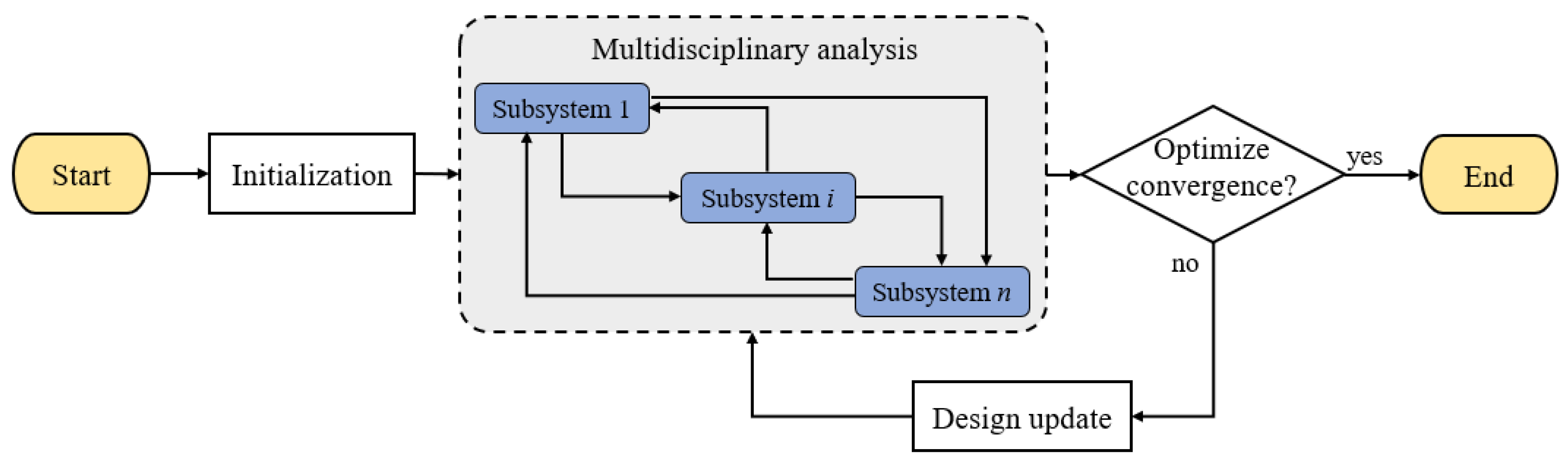
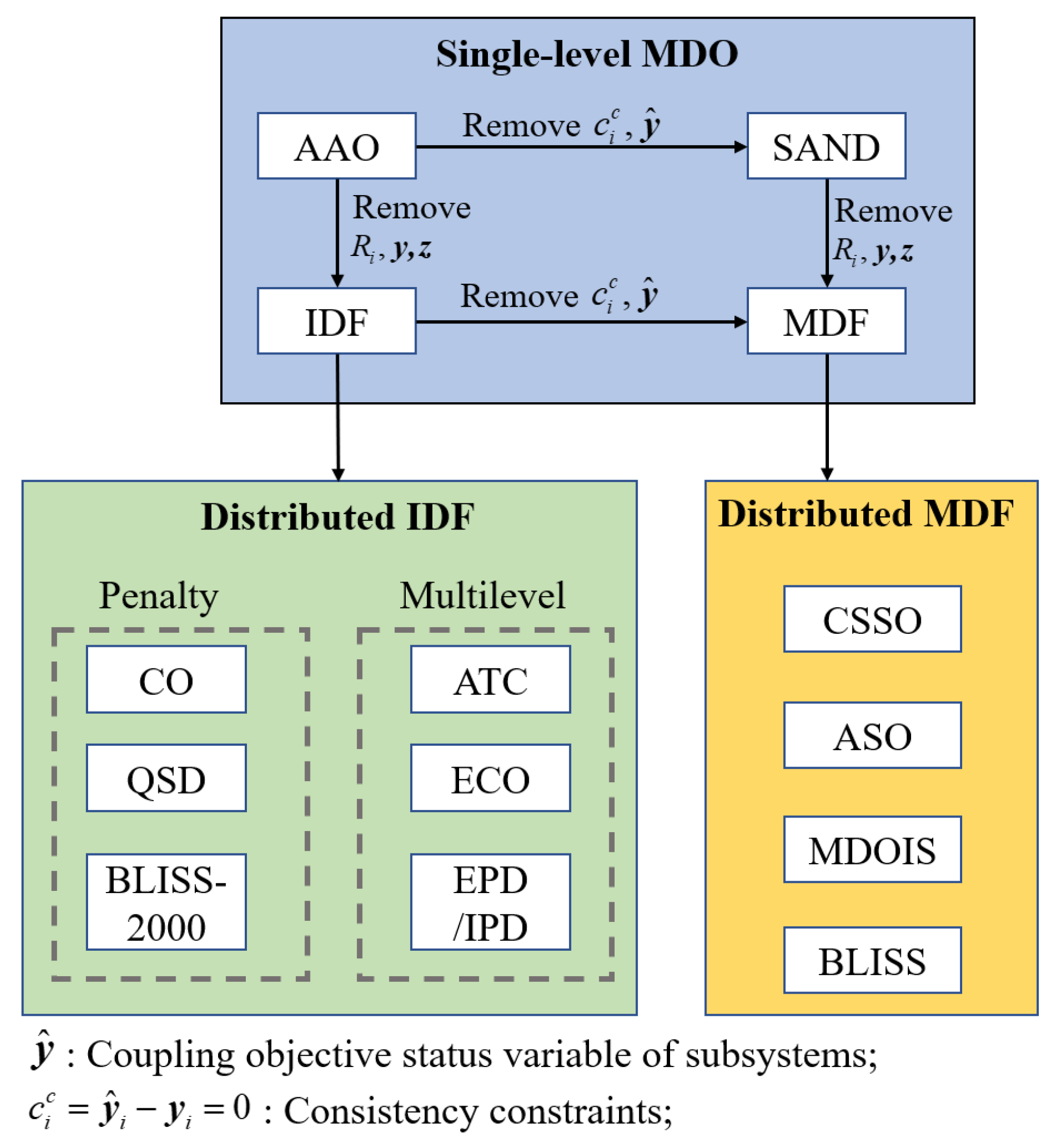
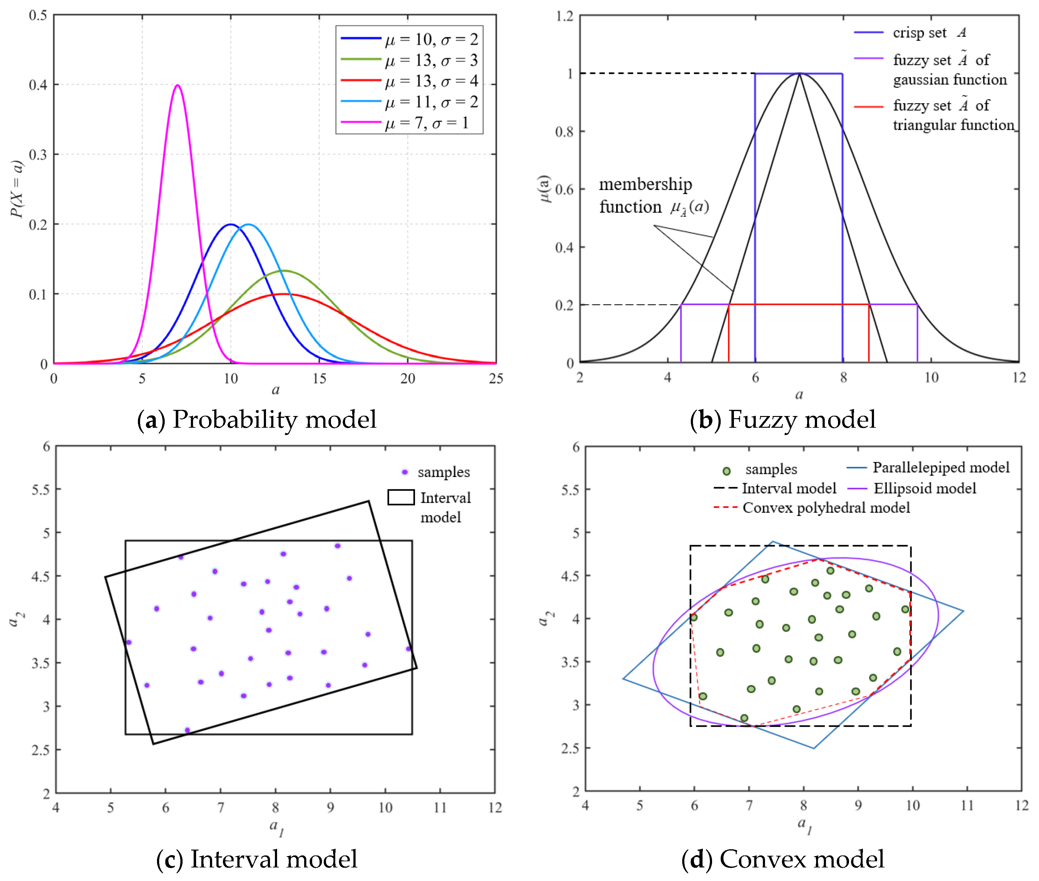
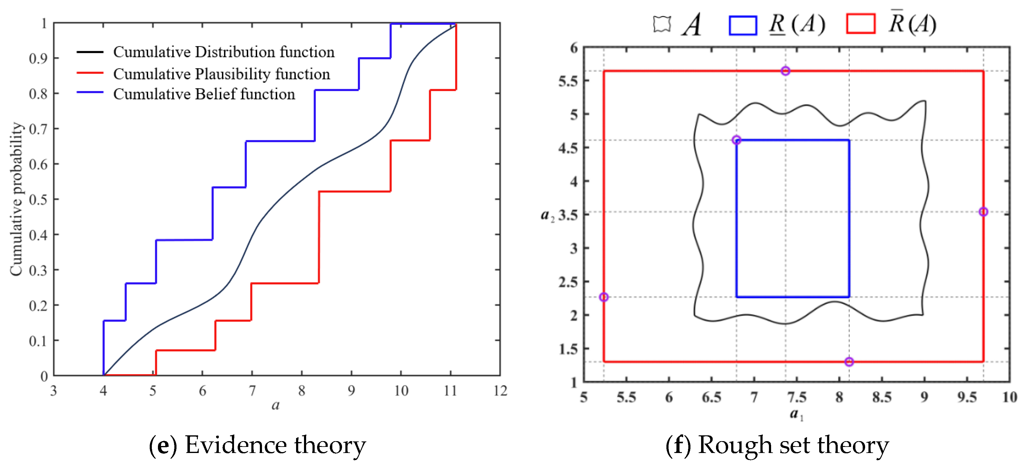
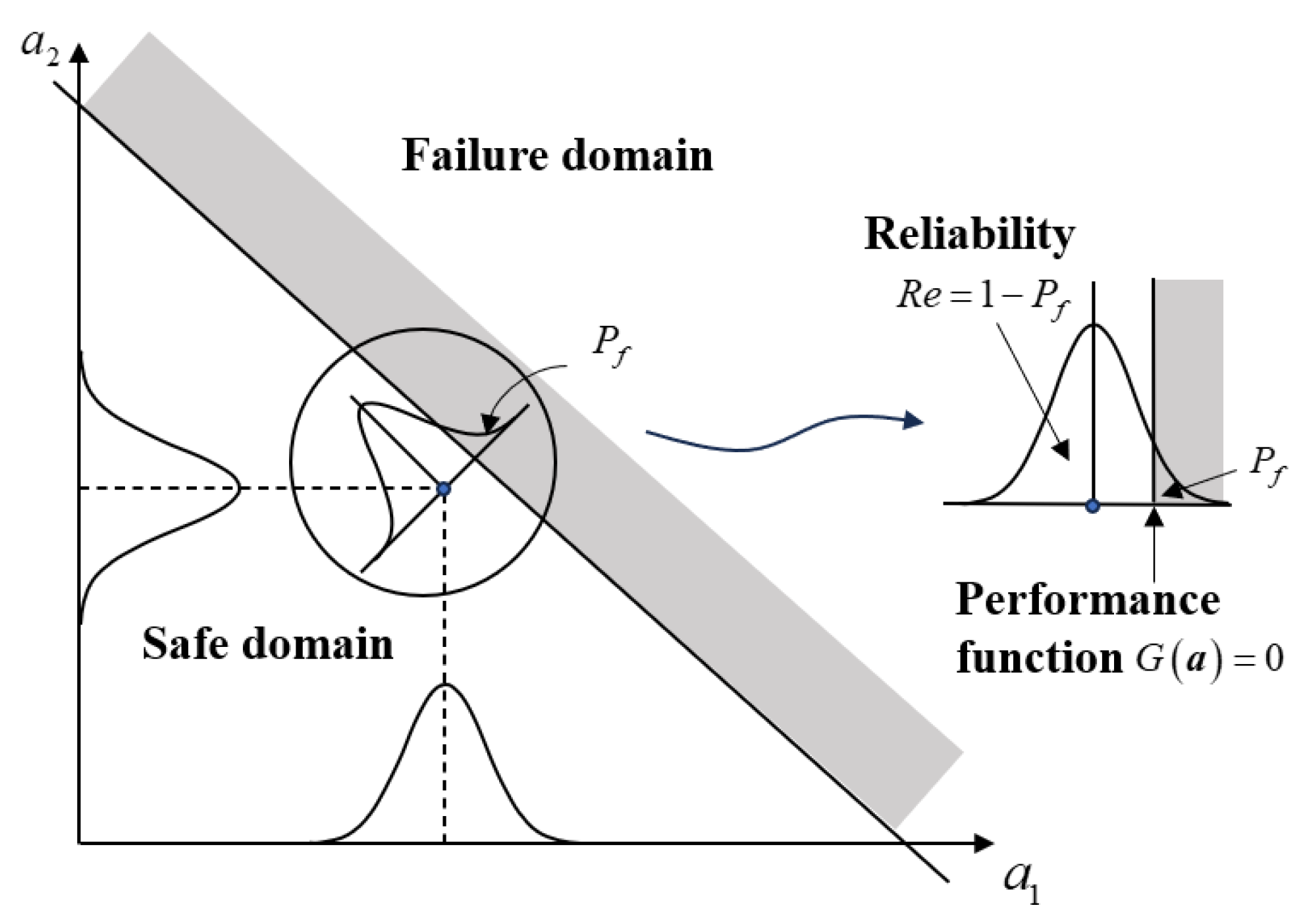
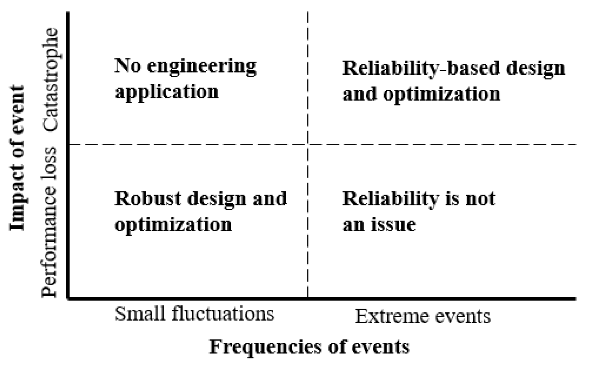
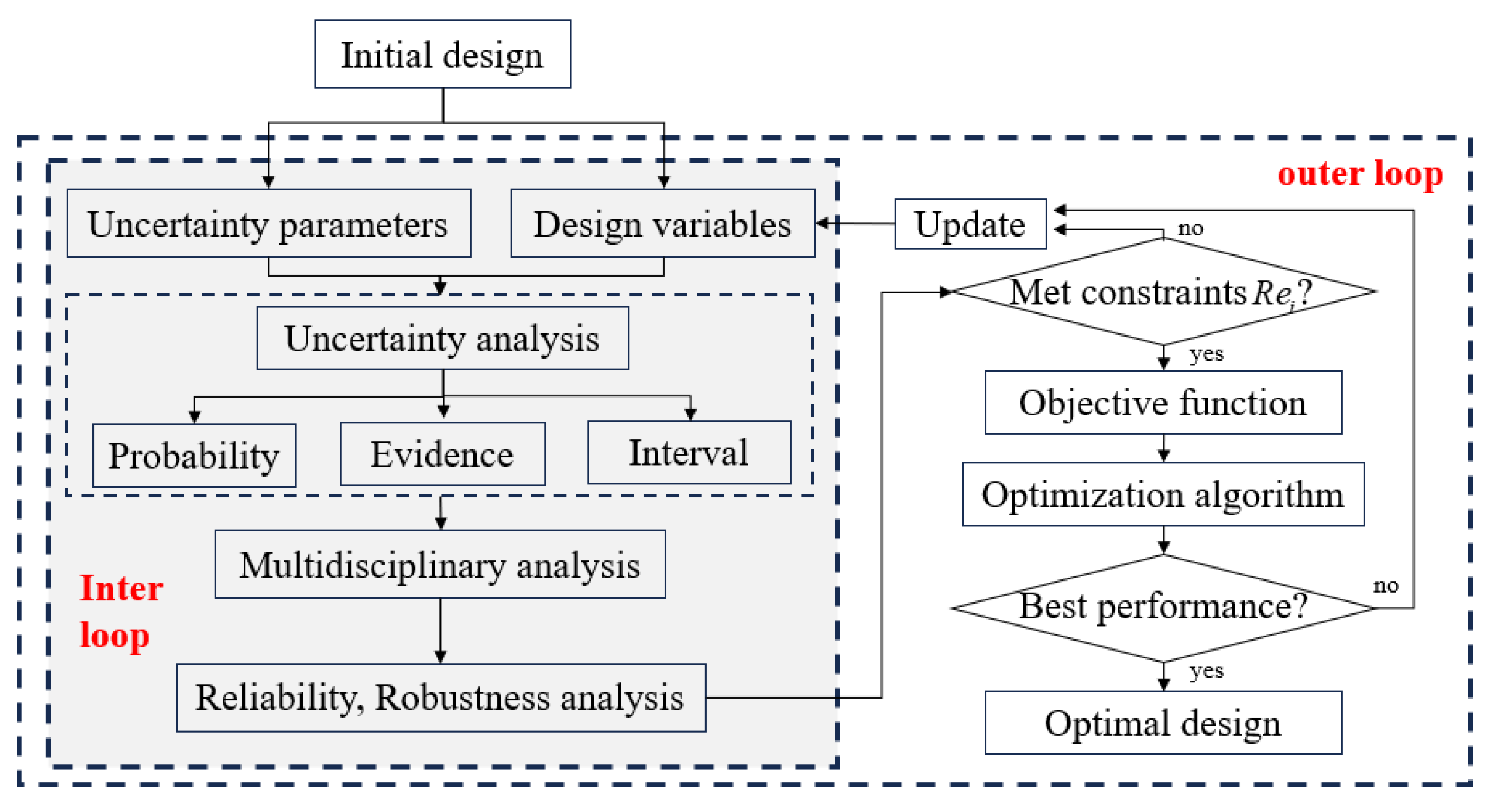
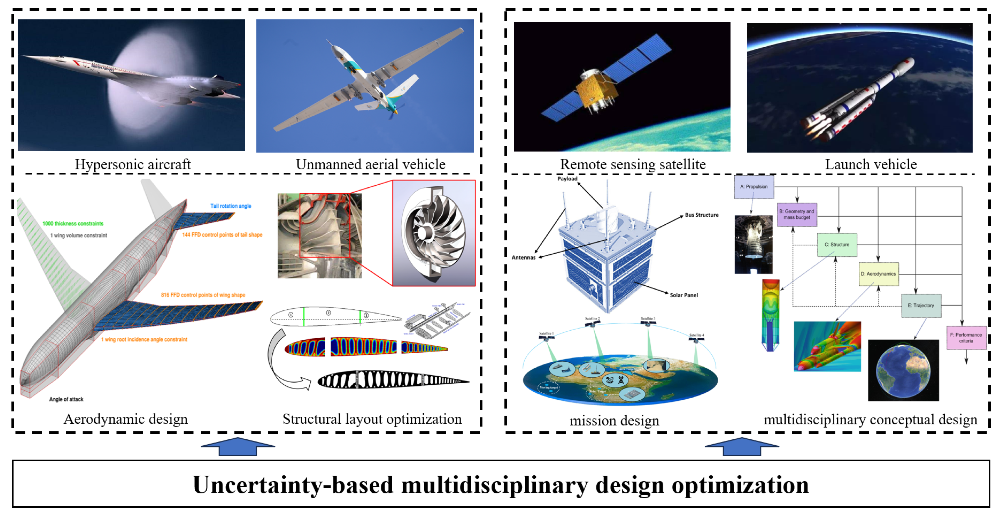
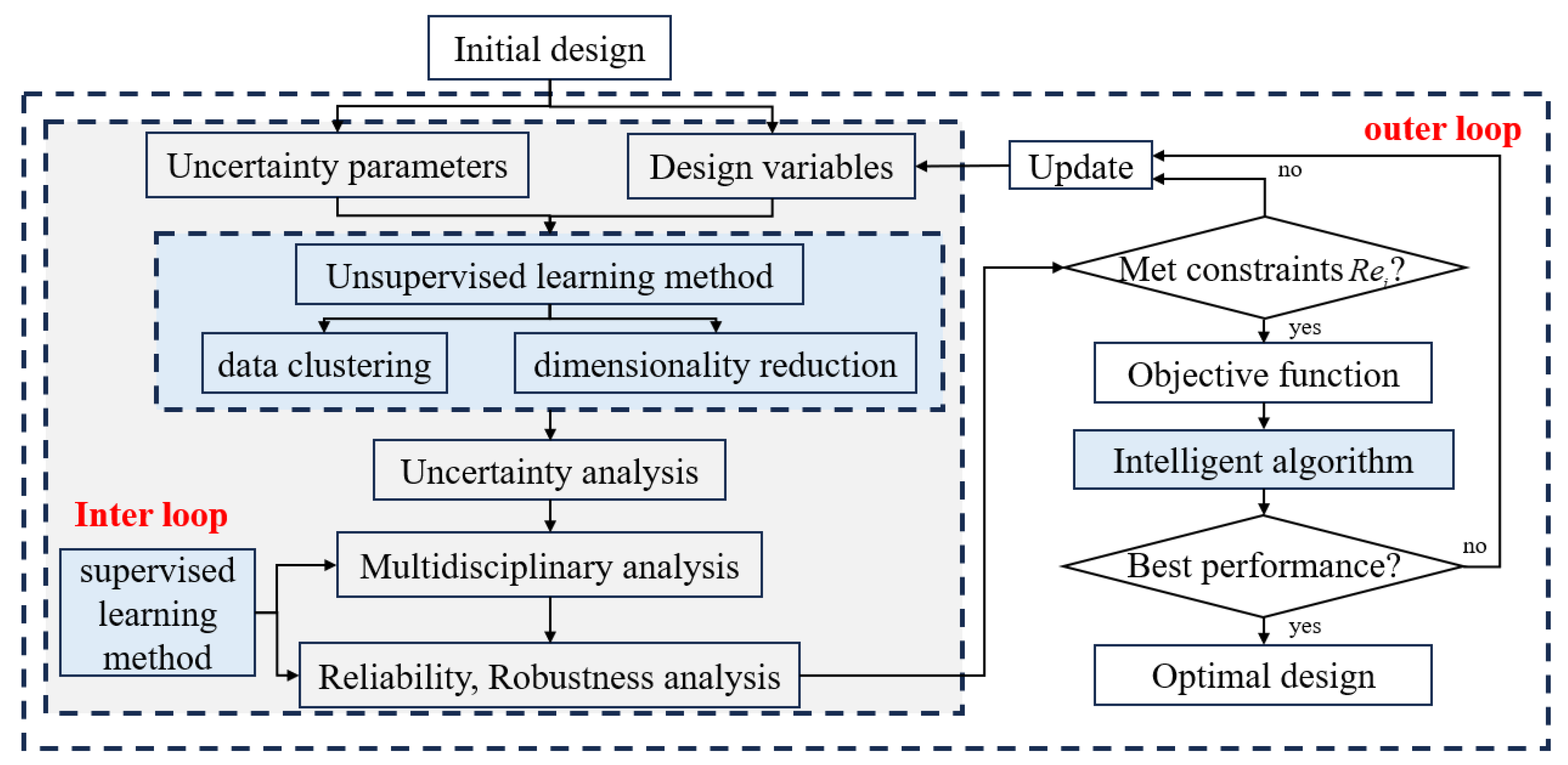
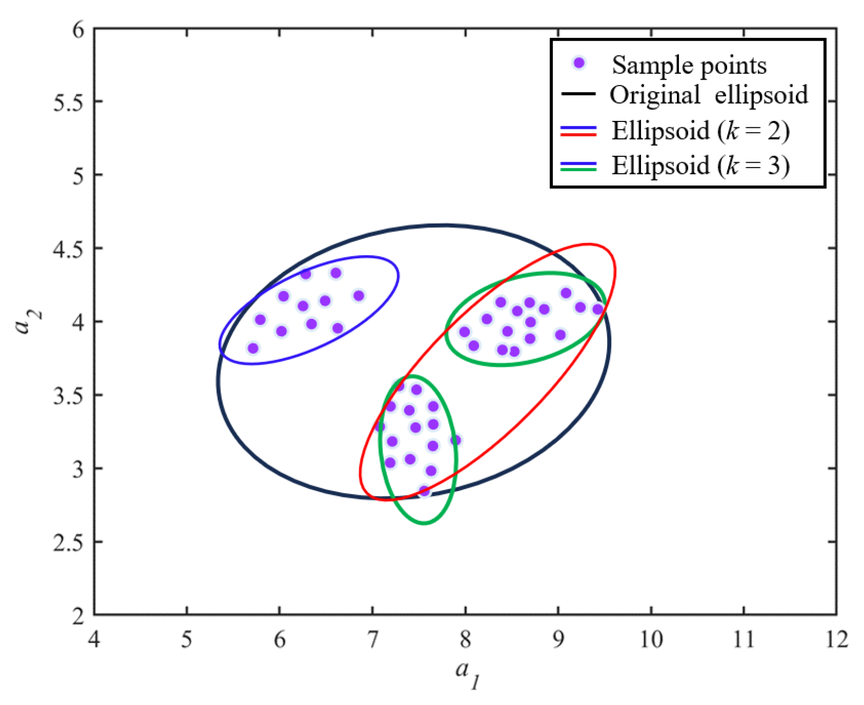
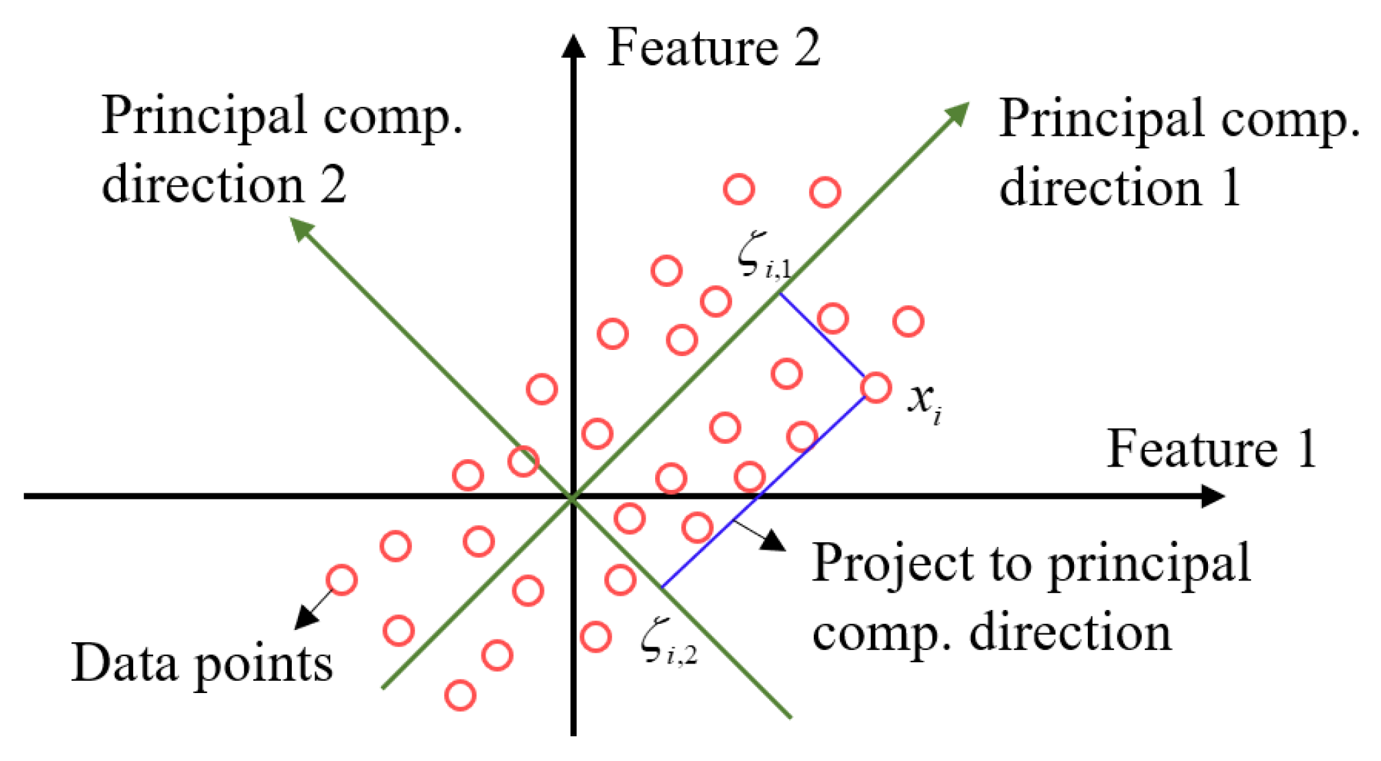
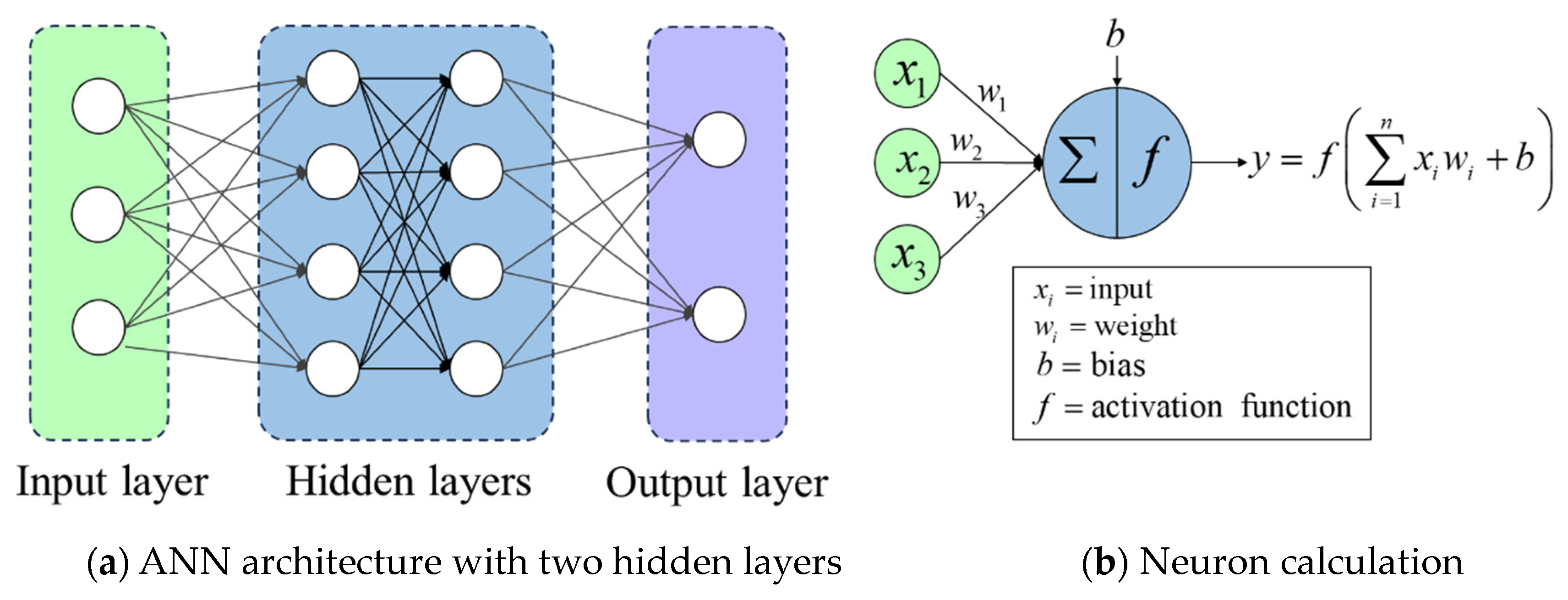
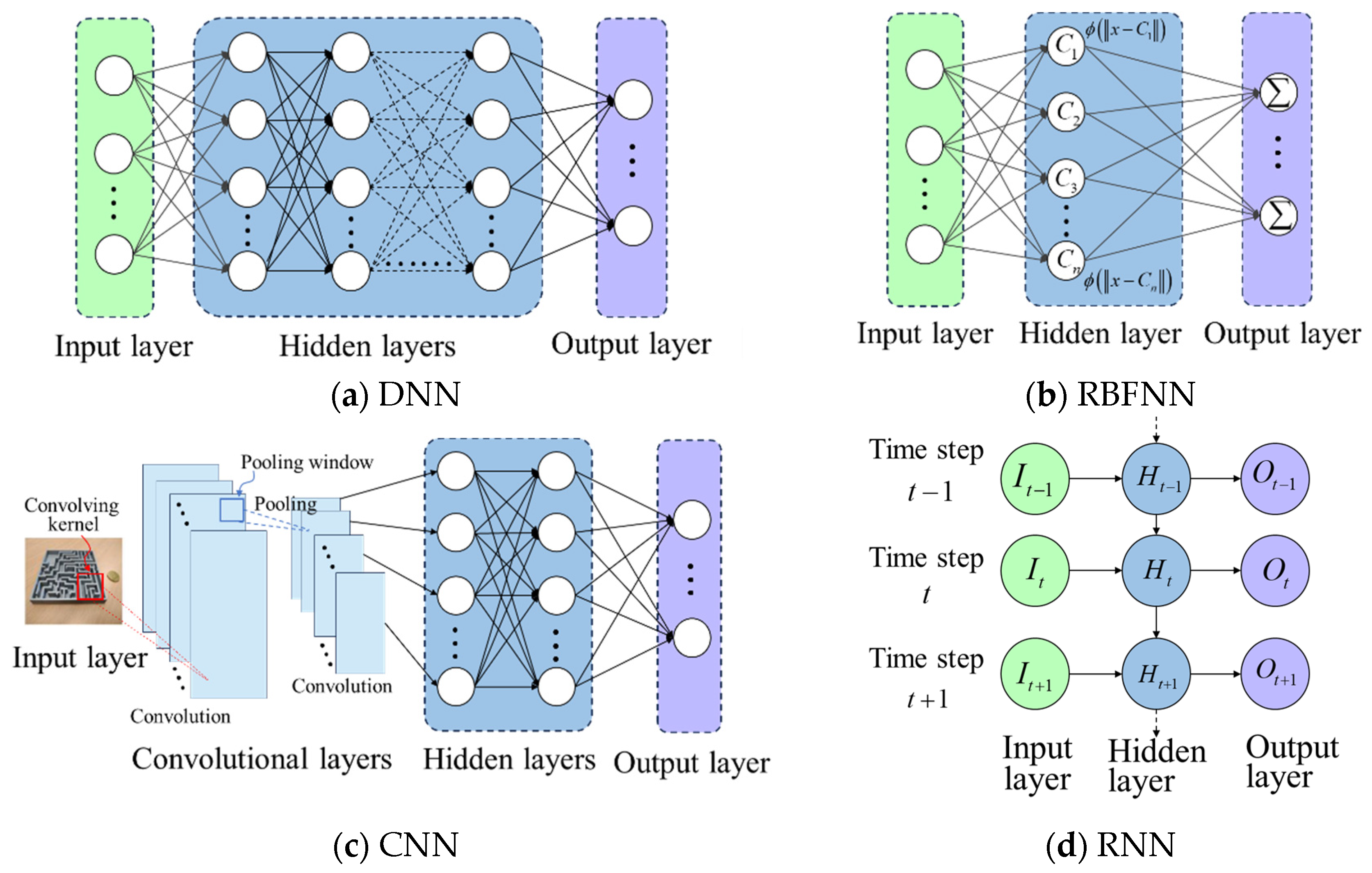
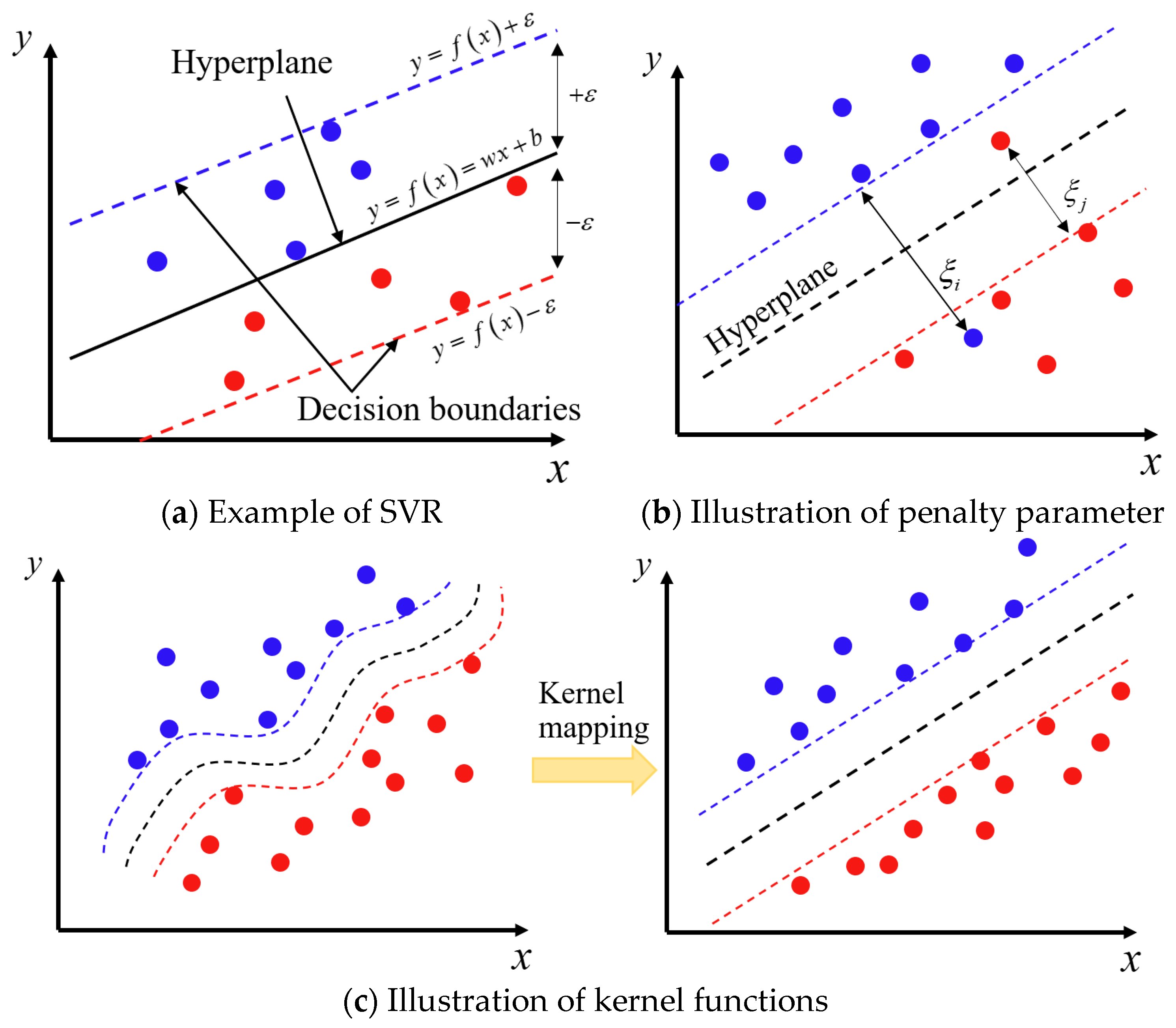
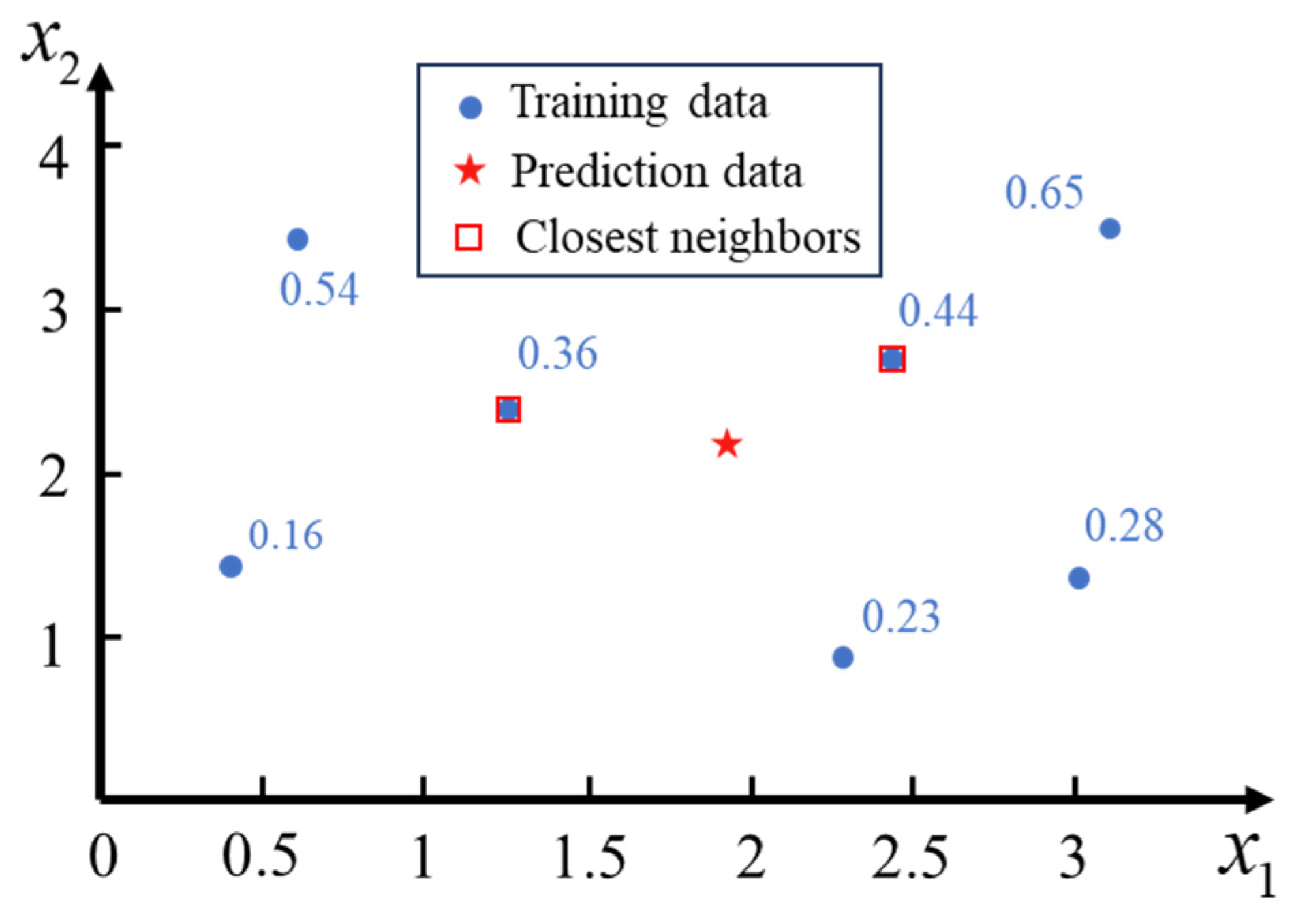
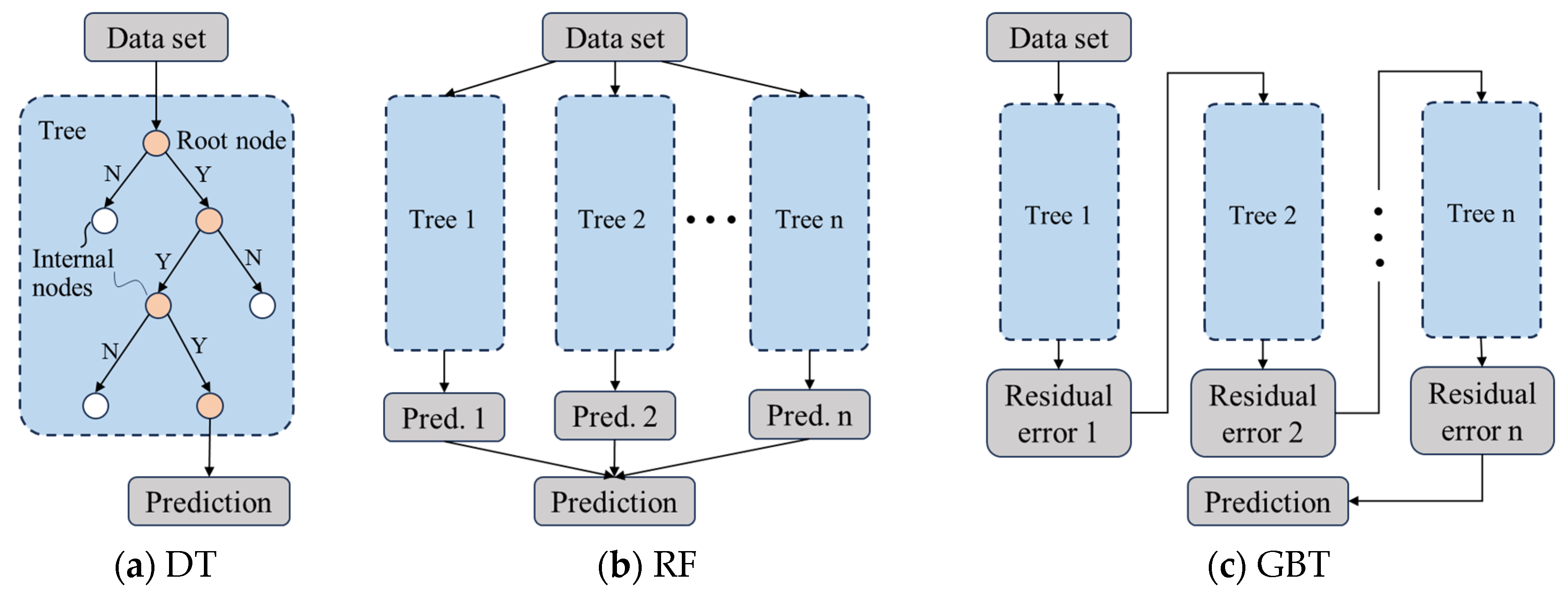
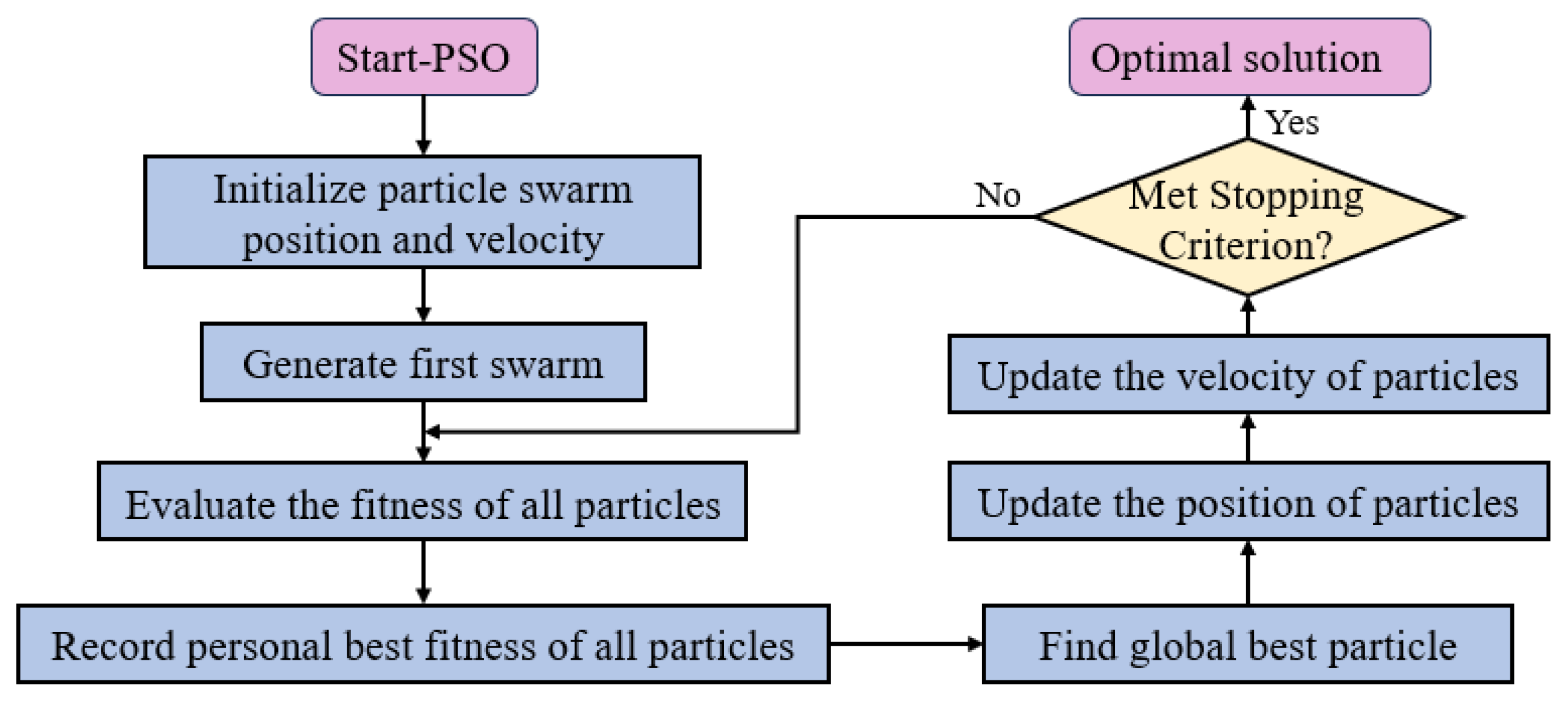
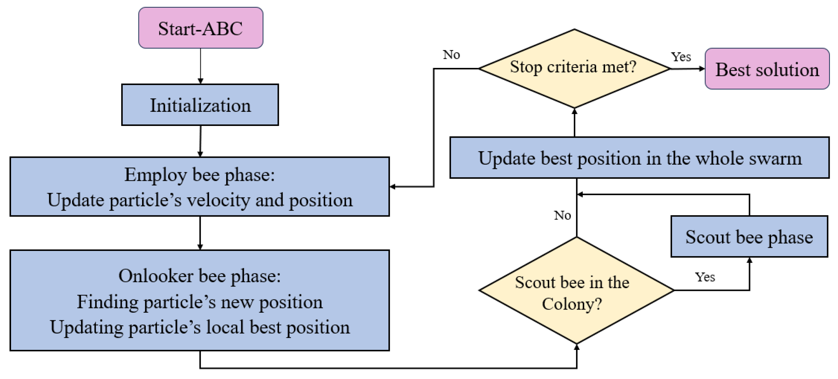
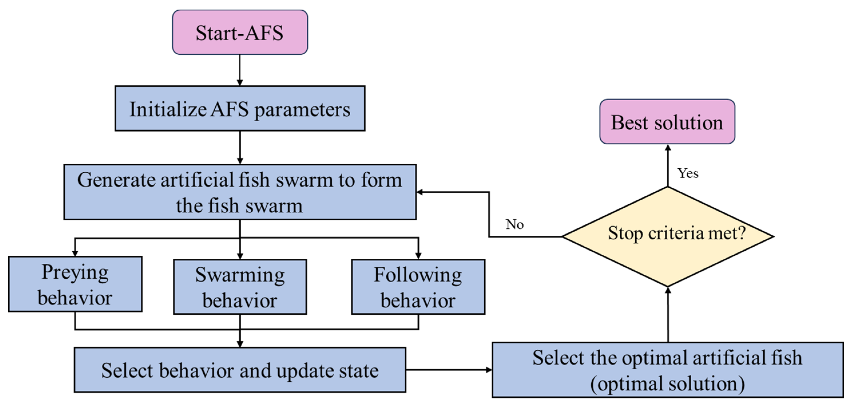
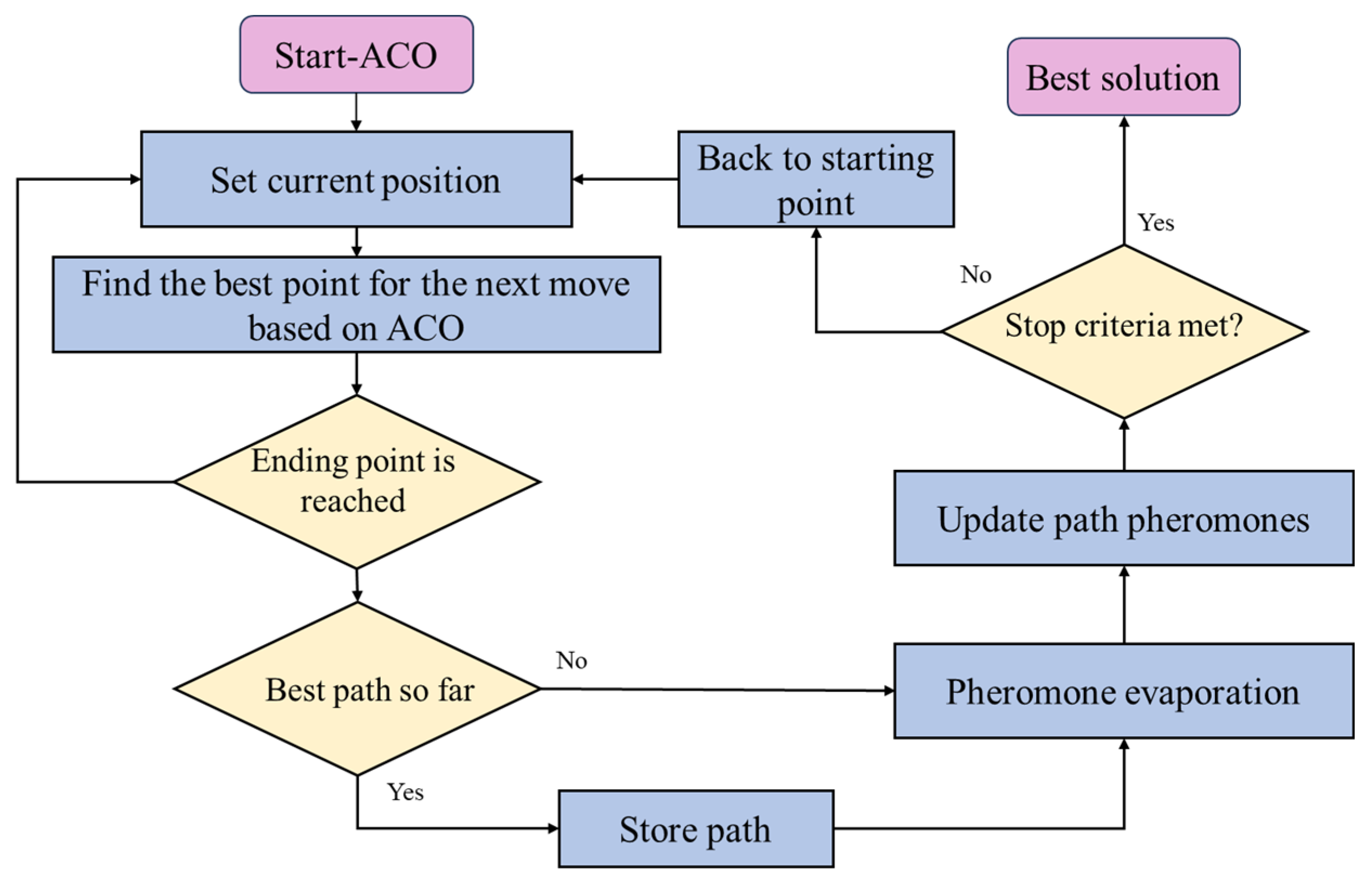
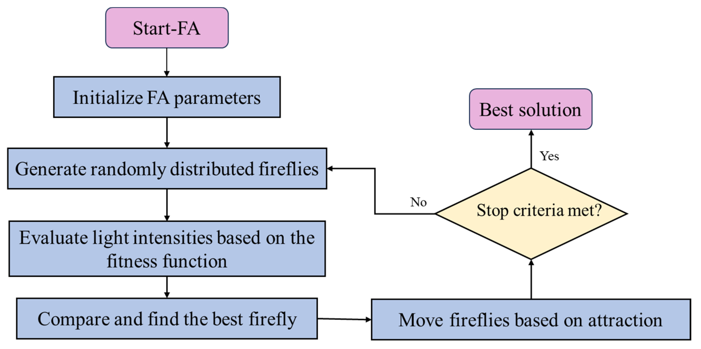
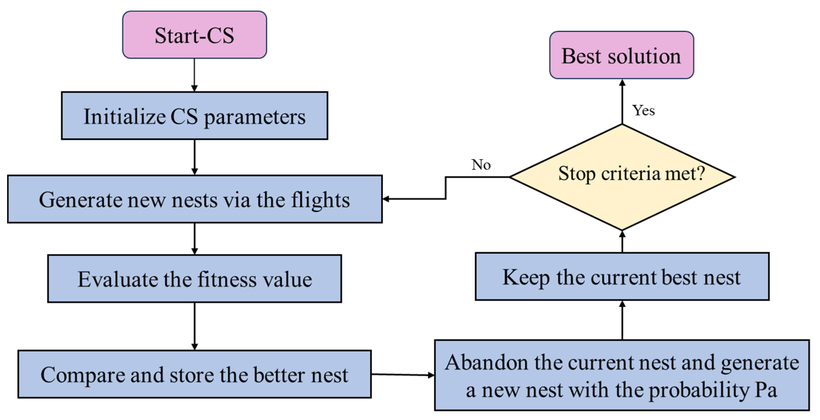
Table 1.
The characteristics of traditional single-level frameworks.
| AAO | MDF | IDF | |
|---|---|---|---|
| Disciplinary feasibility of the solution | At convergence | At each iteration | At each iteration |
| Multidisciplinary feasibility of the solution | At convergence | At each iteration | At convergence |
| Optimized variables | |||
| Convergence speed | Fast | Slow | Medium |
| Advantage | Simple model; able to parallel | Suitable for complex issues | Discipline decoupling; able to parallel |
| Disadvantage | Multiple variables; poor robustness | Need system decomposition | Poor properties in complex issues |
| Application | [21,28,29] | [25,30,31] | [27,32,33] |
Table 2.
The characteristics of typical multi-level architectures.
| CO | CSSO | ATC | BLISS | |
|---|---|---|---|---|
| Efficiency | Low | Fast | Medium | Fast |
| Gradient | No | No | No | Yes |
| Approximate model | Permissible | Necessary | Permissible | Necessary |
| Advantage | Flexible | Parallelizable | Parallelizable | Flexible |
| Drawback | Convergence instability | Accuracy depends on approximate models | Not suitable for small problems | Accuracy depends on approximate models |
| Application | [35,36] | [46,47] | [53] | [49,50] |
Table 3.
Comparison of uncertainty models.
| Uncertainty Modeling | Advantages | Drawbacks |
|---|---|---|
| Probability theory | Adapted to represent aleatory uncertainty | Need information on each singleton of the subset |
| Combination of information using Bayesian approach | Handle mainly aleatory uncertainty | |
| Evidence theory | Handle both aleatory and epistemic uncertainties | Might be difficult to interpret for design |
| No hypothesis needed on the uncertainty distribution inside subsets | Might be difficult to obtain information from experts | |
| Fuzzy set theory | Concept of membership function and fuzzy set | Difficult to interpret for design |
| Express confidence in uncertainty modeling information | Might be difficult to obtain information from experts | |
| Interval theory | Simplicity of modeling | Limitations in uncertainty description |
| Convex theory | Consider the correlation between uncertainty parameters | Need a reasonable method for constructing convex model |
| Minimize samples for uncertainty quantification | ||
| Rough set theory | Describe arbitrary bounded-but-irregular uncertainty set | Uncertainty propagation analysis is influenced by model approximation |
Table 4.
Summary of swarm intelligence algorithms.
| Algorithm | Characteristics | Advantages | Disadvantages | Application |
|---|---|---|---|---|
| PSO | Bubble-net hunting strategy | Solid robustness | Poor property in solving multidimensional issues | [184,189] |
| High accuracy | Inefficient | |||
| ABC | Role-switching mechanism | Strong ability to jump out of local optima | Dependence on solid parameters | [178] |
| Influenced by pheromone | Good property in solving multidimensional issues | Slow convergence speed | ||
| AFS | Preying, following, random behaviors | Fast convergence speed | Easy to fall into local optima | [190] |
| Dependence on solid parameters | ||||
| ACO | Influenced by pheromone | Good property in solving traversal problems | Easy to fall into local optima | [191] |
| Slow convergence speed | ||||
| FA | Attracted by fluorescence intensity | Solid robustness | Weak ability in reaching global optimum | [192,193] |
| High accuracy | Slow convergence speed | |||
| CS | Cuckoo’s nest parasitic behavior | Fast convergence speed | Easy to fall into local optima | [194] |
Disclaimer/Publisher’s Note: The statements, opinions and data contained in all publications are solely those of the individual author(s) and contributor(s) and not of MDPI and/or the editor(s). MDPI and/or the editor(s) disclaim responsibility for any injury to people or property resulting from any ideas, methods, instructions or products referred to in the content. |
© 2023 by the authors. Licensee MDPI, Basel, Switzerland. This article is an open access article distributed under the terms and conditions of the Creative Commons Attribution (CC BY) license (https://creativecommons.org/licenses/by/4.0/).
Share and Cite
MDPI and ACS Style
Wang, C.; Fan, H.; Qiang, X. A Review of Uncertainty-Based Multidisciplinary Design Optimization Methods Based on Intelligent Strategies. Symmetry 2023, 15, 1875. https://doi.org/10.3390/sym15101875
AMA Style
Wang C, Fan H, Qiang X. A Review of Uncertainty-Based Multidisciplinary Design Optimization Methods Based on Intelligent Strategies. Symmetry. 2023; 15(10):1875. https://doi.org/10.3390/sym15101875
Chicago/Turabian StyleWang, Chong, Haoran Fan, and Xin Qiang. 2023. "A Review of Uncertainty-Based Multidisciplinary Design Optimization Methods Based on Intelligent Strategies" Symmetry 15, no. 10: 1875. https://doi.org/10.3390/sym15101875
Note that from the first issue of 2016, this journal uses article numbers instead of page numbers. See further details here.