Article

An Extended TODIM Method and Applications for Multi-Attribute Group Decision-Making Based on Bonferroni Mean Operators under Probabilistic Linguistic Term Sets

1
School of Mathematics and Physics, Anhui Jianzhu University, Hefei 230601, China
2
School of Management, Hefei University of Technology, Hefei 230009, China
3
School of Mathematics and Statistics, Huangshan University, Huangshan 245041, China
*
Author to whom correspondence should be addressed.
Symmetry 2023, 15(10), 1807; https://doi.org/10.3390/sym15101807
Submission received: 25 August 2023 / Revised: 15 September 2023 / Accepted: 18 September 2023 / Published: 22 September 2023
(This article belongs to the Special Issue Fuzzy Set Theory and Uncertainty Theory—Volume II)

Abstract

:
Due to the complexity and uncertainty of decision-making, probabilistic linguistic term sets (PLTSs) are currently important tools for qualitative evaluation of decision-makers. The asymmetry of evaluation information can easily lead to the loss of subjective preference information for decision-makers, and the existing operation of decision-maker evaluation information fusion operators is difficult to solve this problem. To solve such problems, this paper proposes some new operational methods for PLTSs based on Dombi T-conorm and T-norm. Considering the interrelationships between the input independent variables of PLTSs, the probabilistic linguistic weighted Dombi Bonferroni mean Power average (PLWDBMPA) operators are extended and the properties of these aggregation operators are proposed. Secondly, the PLWDBMPA operator is used to fuse the evaluation information of decision-makers, avoiding the loss of decision information as much as possible. This paper uses social media platforms and web crawler technology to obtain online comments from users on decision-making to obtain the public’s attitude towards decision events. TF-IDF and Word2Vec are used to calculate the weight of alternatives on each attribute. Under traditional group decision-making methods and integrating the wisdom of the public, a novel multi-attribute group decision-making method based on TODIM method is proposed. Finally, the case study of Turkey earthquake shelter selection proves this method is scientific and effective. Meanwhile, the superiority of this method was further verified through comparisons with the PL-TOPSIS, PLWA, SPOTIS and PROMETHEE method.

1. Introduction

Multi-criteria decision making (MCDM) is employed to make decisions based on a variety of criteria determining whether or not each alternative is acceptable, considering the complexity of the decision making (DM) process, preferences of decision makers (DMs), conflicting criteria and sources of uncertainty. Multi-attribute group decision making (MAGDM) is an integral part of MCDM [1,2,3,4,5,6,7]. Ziemba [8] proposed the dynamic multi-criteria decision making (DMCDM) methodology for dynamic energy security assessment. Ahmad [9] proposed a multi-choice best–worst method (MCBWM), which takes various alternatives into account when comparing preferences between the criteria in pairs. Zavadskas [10] developed an integrated fuzzy MCDM model to select orders.
The current study on information aggregation is based on a variety of operational rules, including Einstein operation, Hamacher operation, and Frank operation. These research findings are connected to lots of application fields. Dombi operation [11], which is essential generalizations of existing operations, is more flexible than existing operations in terms of collecting information and making decisions because it includes a parameter reflecting the decision-makers’ subject preference. To address DM problems, Liu [12] recently proposed some Dombi Bonferroni mean operators under intuitionistic fuzzy set. Xu [13] extended the Dombi operations to hesitant fuzzy set and devised a variety of aggregation operators. Nevertheless, the current state of research reveals a gap in the field of probabilistic linguistic term set under Dombi operations. Therefore, it is crucial and imperative to conduct research on probabilistic linguistic Dombi operations and employ them to solve MAGDM problems.
Within the process of aggregating information, the Bonferroni mean (BM) method, which was first developed by Bonferroni [14], is utilized to explore the relationships among the input arguments. This approach has been effectively employed in the MCDM. These research endeavors conducted by BM have seen significant development during the past few decades. Xu and Yager [15], for example, extended the BM to the intuitionistic fuzzy set.
Liang [16] combined BM with Grey Relational Analysis method to solve MAGDM problems. Zhu [17] extended BM to the hesitant fuzzy sets. The PLTSs has to demonstrate the relationship between the input arguments since it also confronts the interrelationship phenomenon. We therefore bring BM into the probabilistic linguistic environment while taking into account the special characters of BM [17].
Methods of MADM are crucial in making purchase decisions, which have been extended to several practical applications in a variety of fields, such as TOPSIS [18,19], VIKOR [20,21], ELECTRE [22,23], PROMETHEE [24,25,26,27], SPOTIS [28,29], COMET [30], SIMUS [31], and TOPSI-DARIA [32]. Nevertheless, a common limitation of these methods is their failure to account for the restricted rationality of decision makers. To address this limitation, Gomes and Lima [33] devised a TODIM method that could take into account the constrained rationality on the basis of prospect theory. Liu [34] conducted a hybrid fuzzy TODIM-ERA method under intuitionistic fuzzy sets. Liu [35] combined Analytic Network Process with TODIM method under the Z-information environment. Fan [36] extended the Exponential TODIM method to probabilistic uncertain linguistic term sets.
Around the world, there have been several significant natural disasters in recent years that have resulted in significant losses of people and property. Of all the natural disasters induced by hazards, earthquakes are the most horrific and destructive, and they could conceivably result in immeasurable environmental harm, construction damage, human casualties and population relocation [37]. Houses and infrastructure are destroyed or damaged by earthquakes, necessitating the construction of temporary structures to provide shelter for disaster-affected individuals [38]. Trivedi [39], for instance, proposed a MCDM model to assess determinants of shelter site selection on the basis of decision-making trial and evaluation laboratory (DEMATEL). Xu [40] devised a two-stage consensus reaching model and employed it to the selection of earthquake shelter. Song [41] devised a method that incorporates the advantage of the qualitative flexible multiple criteria (QUALIFLEX) method with the uncertainty inherent in sustainable shelter-site selection.
A novel approach for MAGDM based on new Dombi operational rules under PLTSs and the probabilistic linguistic weighted Dombi Bonferroni mean power average (PLWDBMPA) operator is proposed in this paper. The following are the innovations and advantages of this paper: (1) the online comments of large groups of users and the evaluation information of experts about alternatives are fused to improve the results of MAGDM to be more scientific; (2) the introduction of BM operator and Dombi operation, distinguished from other methods, which not only take into account the decision-makers’ subject preference, but also considering the relationship between the input arguments; (3) the extension of the BM operators under PLTSs to utilize the definition of Dombi and develop some operations, which can be applied to other fuzzy sets like intuitionistic fuzzy set, q-rung ortho pair fuzzy set and spherical fuzzy set.
The rest of this paper is organized as follows. Section 2 presents preliminaries. Section 3 proposes some aggregation operators. Section 4 provides a novel extension model and design an approach for the application of PLMAGDM utilizing the PLWBMPA operator. Section 5 provides an illustrative example to verify the validity of proposed method and compares the proposed method in this paper with the PL-TOPSIS method and the PLWA method. Section 6 summarizes the conclusions of this study.

2. Preliminaries

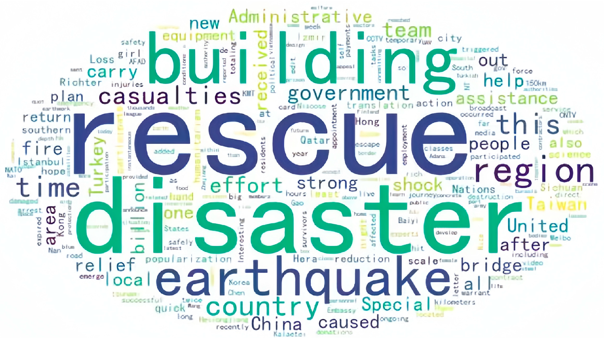
2.1. Keyword Extraction Technique

TF-IDF (term frequency-inverse document frequency) is widely used to determine the keyword weight and evaluate the importance of the extracted words in the field of data mining [42].
The formula for the weight of the extracted words is as Equation (1):
T F I D F ( T ) = t d d ( T ) log ( N / d f ( T ) )
where t d d ( T ) indicates the frequency of the word in the text; N is the number of all texts; d f ( T ) indicates the number of texts containing the word T in the text collection.

2.2. Probabilistic Linguistic Term Sets

Definition 1
[43]. Let S = S τ , S τ + 1 , , S τ 1 , S τ be a linguistic term set, then a PLTS can be defined as Equation (2):
L ( P ) = L ( k ) ( P ( k ) ) | L ( k ) S , P ( k ) 0 , k = 1 , 2 , , # L ( P ) , k = 1 # L ( P ) P ( k ) 1
where L ( k ) ( P ( k ) ) represents the linguistic term L ( k ) with regard to the probability P ( k ) , L ( k ) is the k t h linguistic terms of L ( P ) and # L ( P ) is the number of all different linguistic terms in L ( P ) .
According to the definition in reference [43], all the L ( P ) below are ordered and standardized in the normalization of PLTSs.
Definition 2
[43]. Let L ( P ) = L ( k ) ( P ( k ) ) | k = 1 , 2 , , # L ( P ) and r ( k ) be the subscript of the linguistic term L ( k ) , then the score of L ( P ) is as Equation (3):
E ( L ( P ) ) = S α ¯
where α ¯ = k = 1 # L ( P ) r ( k ) P ( k ) / k = 1 # L ( P ) P ( k ) . For two PLTSs L 1 ( P 1 ) = L ( k ) ( P 1 ( k ) ) | k = 1 , 2 , , # L 1 ( P 1 ) and L 2 ( P 2 ) = L ( l ) ( P 2 ( l ) ) | l = 1 , 2 , , # L 2 ( P 2 ) , if E ( L 1 ( P 1 ) ) > E ( L 2 ( P 2 ) ) , then L 1 ( P 1 ) is superior to L 2 ( P 2 ) , denoted by L 1 ( P 1 ) > L 2 ( P 2 ) ; if E ( L 1 ( P 1 ) ) < E ( L 2 ( P 2 ) ) , then L 2 ( P 2 ) is superior to L 1 ( P 1 ) , denoted by L 1 ( P 1 ) < L 2 ( P 2 ) . However, if E ( L 1 ( P 1 ) ) = E ( L 2 ( P 2 ) ) , the degree of deviation needs to be further defined.
Definition 3
[43]. Let L ( P ) = L ( k ) ( P ( k ) ) | k = 1 , 2 , , # L ( P ) and r ( k ) be the subscript of the linguistic term L ( k ) , where α ¯ = k = 1 # L ( P ) r ( k ) P ( k ) / k = 1 # L ( P ) P ( k ) . Then the deviation of degree L ( P ) is as Equation (4):
σ ( L ( P ) ) = k = 1 # L ( P ) P ( k ) r ( k ) α ¯ 2 / k = 1 # L ( P ) P ( k )
where E ( L 1 ( P 1 ) ) = E ( L 2 ( P 2 ) ) , if σ ( L 1 ( P 1 ) ) > σ ( L 2 ( P 2 ) ) , then L 1 ( P 1 ) < L 2 ( P 2 ) ; if σ ( L 1 ( P 1 ) ) < σ ( L 2 ( P 2 ) ) , then L 1 ( P 1 ) > L 2 ( P 2 ) ; however, if σ ( L 1 ( P 1 ) ) = σ ( L 2 ( P 2 ) ) , then L 1 ( P 1 ) is indifferent to L 2 ( P 2 ) , denoted by L 1 ( P 1 ) L 2 ( P 2 ) .
Definition 4
[44]. Let S = S τ , S τ + 1 , , S τ 1 , S τ be a linguistic term set, L ( P ) is a PLTS. The equivalent transformation function of L ( P ) is defined as Equation (5):
g L ( P ) = α ( k ) + τ 2 τ P ( k ) = L ϖ ( P ) ,
where g : [ τ , τ ] [ 0 , 1 ] and ϖ [ 0 , 1 ] . Additionally, we can obtain the transformation function of L ϖ ( P ) as Equation (6):
g 1 L ϖ ( P ) = s ϖ τ P ( k ) | ϖ [ 0 , 1 ] = L ( P ) .
where g 1 : [ 0 , 1 ] [ τ , τ ] .
Definition 5
[43]. There are two PLTSs L 1 ( P 1 ) = L ( k ) ( P 1 ( k ) ) | k = 1 , 2 , , # L 1 ( P 1 ) and L 2 ( P 2 ) = L ( l ) ( P 2 ( l ) ) | l = 1 , 2 , , # L 2 ( P 2 ) , # L 1 ( P 1 ) = # L 2 ( P 2 ) . The deviation degree between L 1 ( P 1 ) and L 2 ( P 2 ) is defined as Equation (7):
d ( L 1 ( P 1 ) , L 2 ( P 2 ) ) = 1 # L 1 ( P 1 ) j = 1 # L 1 ( P 1 ) P 1 ( j ) g L 1 ( j ) P 2 ( j ) g L 2 ( j ) 2 1 2
where g L 1 ( j ) = r 1 ( j ) + τ 2 τ , g L 2 ( j ) = r 2 ( j ) + τ 2 τ . r 1 ( j ) and r 2 ( j ) are the subscripts of linguistic terms L ( k ) and L ( l ) respectively.
Definition 6
[11]. Let λ be a parameter, λ > 0 and x , y [ 0 , 1 ] , the Dombi T-norm and T-conorm are defined as Equations (8) and (9):
T D , λ x , y = 1 1 + 1 x x λ + 1 y y λ 1 / λ
T D , λ * x , y = 1 1 1 + x 1 x λ + y 1 y λ 1 / λ
Recently, Liu [12] developed the Dombi operation for intuitionistic fuzzy numbers (IFNs). Under Dombi T-norm and T-conorm, Xu [13] extended the Dombi operations to hesitant fuzzy set. We give some Dombi operations for PLTSs based on the findings of the previous research.
Definition 7.
Let S = S τ , S τ + 1 , , S τ 1 , S τ be a linguistic term set, L ( P ) , L 1 ( P 1 ) and L 2 ( P 2 ) be three PLTSs, and δ be a positive real numbers. η ( k ) g L , η 1 ( i ) g L 1 , η 2 ( j ) g L 2 and k = 1 , 2 , , # L ( P ) , i = 1 , 2 , , # L 1 ( P 1 ) , j = 1 , 2 , , # L 2 ( P 2 ) where   g is the equivalent transformation function. The Dombi operations are defined as follows:
L 1 ( P 1 ) L 2 ( P 2 ) = g 1 η 1 ( i ) g ( L 1 ) , η 2 ( j ) g ( L 2 ) 1 1 1 + η 1 ( i ) 1 η 1 ( i ) λ + η 2 ( j ) 1 η 2 ( j ) λ 1 / λ P 1 ( i ) P 2 ( j )
L 1 ( P 1 ) L 2 ( P 2 ) = g 1 η 1 ( i ) g ( L 1 ) , η 2 ( j ) g ( L 2 ) 1 1 + 1 η 1 ( i ) η 1 ( i ) λ + 1 η 2 ( j ) η 2 ( j ) λ 1 / λ P 1 ( i ) P 2 ( j )
δ L ( P ) = g 1 η ( k ) g ( L ) 1 1 1 + δ η ( k ) 1 η ( k ) λ 1 / λ P ( k )
L ( P ) δ = g 1 η ( k ) g ( L ) 1 1 + δ 1 η ( k ) η ( k ) λ 1 / λ P ( k )
Theorem 1.
Let S = S τ , S τ + 1 , , S τ 1 , S τ be a linguistic term set, L ( P ) , L 1 ( P 1 ) , and L 2 ( P 2 ) be three PLTSs, and δ , δ 1 , δ 2 be three positive real numbers. Then
(1)
L 1 ( P 1 ) L 2 ( P 2 ) = L 2 ( P 2 ) L 1 ( P 1 )
(2)
L 1 ( P 1 ) L 2 ( P 2 ) = L 2 ( P 2 ) L 1 ( P 1 )
(3)
δ L 1 ( P 1 ) L 2 ( P 2 ) = δ L 1 ( P 1 ) δ L 2 ( P 2 )
(4)
L 1 ( P 1 ) L 2 ( P 2 ) δ = L 1 ( P 1 ) δ L 2 ( P 2 ) δ
(5)
δ 1 L ( P ) δ 2 L ( P ) = δ 1 + δ 2 L ( P )
(6)
L ( P ) δ 1 L ( P ) δ 2 = L ( P ) δ 1 + δ 2 .
The proof of Theorem 1 is given in Appendix A.

2.3. Bonferroni Mean (BM) and Power Average (PA)

Definition 8
[14]. Let p , q 0 and X = x 1 , x 2 , x n be a collection of non-negative numbers. Then the Bonferroni Mean is defined as Equation (14):
B p , q X = 1 n ( n 1 ) i , j = 1 , i j n x i p x j q 1 p + q
Definition 9
[45]. Let A = a 1 , a 2 , a n be a collection of non-negative numbers. Then the power aggregation is defined as Equation (15):
P A a 1 , a 2 , , a n = i = 1 n 1 + T a i i = 1 n 1 + T a i a i
where T ( a i ) = j = 1 , j i n sup ( a i , a j ) and sup ( a i , a j ) is denoted as the support for a i from a j , which satisfies the following properties:
(1)
sup ( a i , a j ) [ 0 , 1 ] ;
(2)
sup ( a i , a j ) = sup ( a j , a i ) ;
(3)
sup ( a i , a j ) sup ( a i , a k ) , i f   d ( a i , a j ) d ( a i , a k ) ;

3. Probabilistic Linguistic Weighted Dombi Bonferroni Mean Power Average Operators

We present the PLDBMPA operator and PLWDBMPA operator under the new PLTSs operational rules, and then investigate their properties in this section.

3.1. PLDBMPA Operators

We explore the fact that the input arguments of GBM given in [14] are PLTSs and then present the PLDBMPA operator as follow.
Definition 10.
Let L i ( P i ) = L i ( k ) ( P i ( k ) ) | k = 1 , 2 , , # L i ( P i )   i = 1 , 2 , , n be n PLTSs. The PLDBMPA operator is defined as Equation (16):
P L D B M P A p , q L 1 ( P 1 ) , L 2 ( P 2 ) , , L n ( P n ) = 1 n ( n 1 ) i , j = 1 i j n ( ( n ( 1 + T ( L i ( P i ) ) ) t = 1 n ( 1 + T ( L t ( P t ) ) ) L i ( P i ) ) p ( n ( 1 + T ( L j ( P j ) ) ) t = 1 n ( 1 + T ( L t ( P t ) ) ) L j ( P j ) ) q ) 1 p + q
where p , q 0 , T ( L i ( P i ) ) = j = 1 , j i n S u p L i ( P i ) , L j ( P j ) , the support degree of L 1 ( P 1 ) and L 2 ( P 2 ) is S u p L i ( P i ) , L j ( P j ) = 1 d L i ( P i ) , L j ( P j ) , which satisfies the following properties:
(1)
S u p L i ( P i ) , L j ( P j ) [ 0 , 1 ] ;
(2)
S u p L i ( P i ) , L j ( P j ) = S u p L j ( P j ) , L i ( P i ) ;
(3)
If d L i ( P i ) , L j ( P j ) < d L i ( P i ) , L l ( P l ) , then S u p L i ( P i ) , L j ( P j ) > S u p L i ( P i ) , L l ( P l ) .
Theorem 2.
Let L i ( P i ) = L i ( k ) ( P i ( k ) ) | k = 1 , 2 , , # L i ( P i ) , i = 1 , 2 , , n be n PLTSs and p , q 0 , then the aggregated value obtained by PLDBMPA operator is still a PLTS, and
P L D B M P A p , q L 1 ( P 1 ) , L 2 ( P 2 ) , , L n ( P n ) = 1 n ( n 1 ) i , j = 1 i j n ( ( n ( 1 + T ( L i ( P i ) ) ) t = 1 n ( 1 + T ( L t ( P t ) ) ) L i ( P i ) ) p ( n ( 1 + T ( L j ( P j ) ) ) t = 1 n ( 1 + T ( L t ( P t ) ) ) L j ( P j ) ) q ) 1 p + q = η i ( k ) g ( L i ) , η j ( d ) g ( L j ) g 1 1 + n ( n 1 ) ( p + q ) i = 1 n j = 1 j i n p E i K i λ + q E j D j λ 1 1 1 / λ 1 Π i , j = 1 i j n P i ( k ) P j ( d )
where E i = n ( 1 + T ( L i ( P i ) ) ) t = 1 n ( 1 + T ( L t ( P t ) ) ) , E j = n ( 1 + T ( L j ( P j ) ) ) t = 1 n ( 1 + T ( L t ( P t ) ) ) , K i = 1 η i ( k ) η i ( k ) , D j = 1 η j ( d ) η j ( d ) .
The proof of Theorem 2 is given in Appendix B.
The corollaries of P L D B M P A p , q L 1 ( P 1 ) , L 2 ( P 2 ) , , L n ( P n ) for Theorem 1 based on the results of Reference [16] are as follows.
Corollary 1.
Commutativity, If L i ( P i ) is any permutation of L i ( P i )   i = 1 , 2 , , n , we then obtain the relationship:
P L D B M P A p , q L 1 ( P 1 ) , L 2 ( P 2 ) , , L n ( P n ) = P L D B M P A p , q L 1 ( P 1 ) , L 2 ( P 2 ) , , L n ( P n )
Corollary 2 (Monotonicity).
Let ε i j = 1 + n ( n 1 ) ( p + q ) i = 1 n j = 1 j i n p E i K i λ + q E j D j λ 1 1 1 / λ 1 , when the values of n , p , q are constant, with regard to the increase of η i ( k ) and η j ( d ) , ε i j is increasing monotonously.

3.2. PLWDBMPA Operators

We propose the Probabilistic Linguistic Weighted Dombi Bonferroni Mean Power Average (PLWDBMPA) operator in this section, with the consideration of importance of aggregated multi-input arguments.
Definition 11.
Let L i ( P i ) = L i ( k ) ( P i ( k ) ) | k = 1 , 2 , , # L i ( P i ) , i = 1 , 2 , , n be n PLTSs and p , q 0 ,   w = ( w 1 , w 2 , , w n ) T is the weight vector of L i ( P i ) , where w i indicates the importance degree of L i ( P i ) , w i 0 , 1 and i n w i = 1 . Then, the PLWDBMPA operator is defined as Equation (18):
P L W D B M P A p , q L 1 ( P 1 ) , L 2 ( P 2 ) , , L n ( P n ) = 1 n ( n 1 ) i , j = 1 i j n ( ( n w i ( 1 + T ( L i ( P i ) ) ) t = 1 n w t ( 1 + T ( L t ( P t ) ) ) L i ( P i ) ) p ( n w j ( 1 + T ( L j ( P j ) ) ) t = 1 n w t ( 1 + T ( L t ( P t ) ) ) L j ( P j ) ) q ) 1 p + q
where T ( L i ( P i ) ) = j = 1 , j i n w j S u p L i ( P i ) , L j ( P j ) , the support degree of L 1 ( P 1 ) and L 2 ( P 2 ) is S u p L i ( P i ) , L j ( P j ) = 1 d L i ( P i ) , L j ( P j ) g = 1 g i n d L i ( P i ) , L g ( P g ) .
Theorem 3.
Let L i ( P i ) = L i ( k ) ( P i ( k ) ) | k = 1 , 2 , , # L i ( P i ) , i = 1 , 2 , , n be n PLTSs and p , q 0 ,   w = ( w 1 , w 2 , , w n ) T is the weight vector of L i ( P i ) , where w i indicates the importance degree of L i ( P i ) , w i 0 , 1 and i n w i = 1 . Then, the aggregated value obtained by the PLWDBMPA operator is still a PLTS, and
P L W D B M P A p , q L 1 ( P 1 ) , L 2 ( P 2 ) , , L n ( P n ) = 1 n ( n 1 ) i , j = 1 i j n ( ( n w i ( 1 + T ( L i ( P i ) ) ) t = 1 n w t ( 1 + T ( L t ( P t ) ) ) L i ( P i ) ) p ( n w j ( 1 + T ( L j ( P j ) ) ) t = 1 n w t ( 1 + T ( L t ( P t ) ) ) L j ( P j ) ) q ) 1 p + q = η i ( k ) g ( L i ) , η j ( d ) g ( L j ) g 1 1 + n ( n 1 ) ( p + q ) i = 1 n j = 1 j i n p v i K i λ + q v j D j λ 1 1 1 / λ 1 Π i , j = 1 i j n P i ( k ) P j ( d )
where v i = n w i ( 1 + T ( L i ( P i ) ) ) t = 1 n w t ( 1 + T ( L t ( P t ) ) ) , v j = n w j ( 1 + T ( L j ( P j ) ) ) t = 1 n w t ( 1 + T ( L t ( P t ) ) ) , K i = 1 η i ( k ) η i ( k ) , D j = 1 η j ( d ) η j ( d ) .

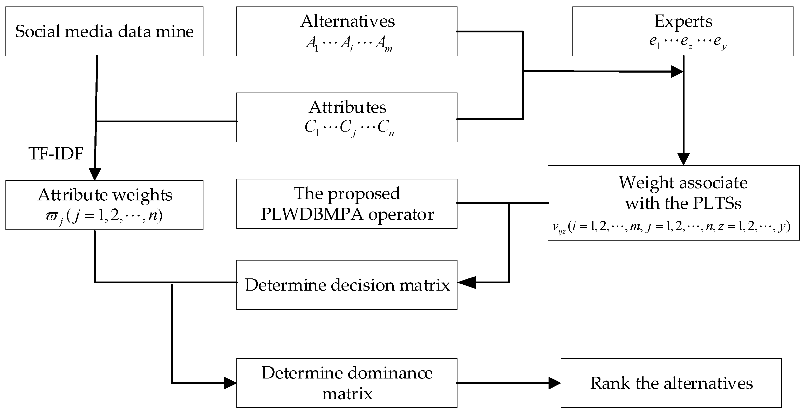
4. Solving Multi-Attribute Group Decision-Making Problem with the PLWDBMPA Operator

4.1. The Problem Description of MAGDM

The PLMAGDM problem contains several decision matrices that provides assessments of all alternatives employing PLTSs for each attribute. Let A = A i | i = 1 , 2 , , m be a discrete set of alternatives and C = C j | j = 1 , 2 , , n be the set of attributes. S = S τ , S τ + 1 , , S τ 1 , S τ be the linguistic term set. Suppose that E = e z | z = 1 , 2 , , y is the set of experts with the corresponding weight information W = ( w 1 , w 2 , , w y ) T where 0 w z 1 , z = 1 y w z = 1 . Let L i j z P i j z be the PLTS converted from the evaluation of expert e z for alternative A i with the attribute C j . Then, let D z = L i j z P i j z m × n be the probabilistic linguistic decision matrix provided by the expert e z ( z = 1 , 2 , , y ) . Hence, the probabilistic linguistic decision matrix D z can be written as:
D z = L 11 z ( P 11 z ) L 12 z ( P 12 z ) L 1 n z ( P 1 n z ) L 21 z ( P 21 z ) L 22 z ( P 22 z ) L 2 n z ( P 2 n z ) L m 1 z ( P m 1 z ) L m 2 z ( P m 2 z ) L m n z ( P m n z )
where the element L i j z ( P i j z ) denotes the evaluation value of the alternative A i according to the attribute C j provided by the expert e z ( i = 1 , 2 , , m ; j = 1 , 2 , , n ) . .
The flowchart of the decision procedure is as Figure 1.

4.2. The Decision Procedure

We propose a novel approach of application for MAGDM with PLWDBMPA and TODIM method based on the results mentioned above. We apply the PLWDBMPA to integrate the information of MAGDM while the TODIM method also can assist us in making decisions. This novel approach is proposed as follows:
Step 1. When it comes to the DM problem, we define the discrete set of alternatives A = A i | i = 1 , 2 , , m and the set of attributes C = C j | j = 1 , 2 , , n . Suppose that E = e z | z = 1 , 2 , , y is the set of experts, their corresponding weight is W = w 1 , w 2 , , w y T , the linguistic term set is S = S τ , S τ + 1 , , S τ 1 , S τ and the probabilistic linguistic decision matrix is constructed as D z = L i j z P i j z m × n ( i = 1 , 2 , , m ; j = 1 , 2 , , n ; z = 1 , 2 , , y ) provided by the expert e z .
Step 2. Determine the weight associated with the PLTSs.
(1)
The deviation degree between L i j z ( P i j z ) = L i j z ( k ) ( P i j z ( k ) ) | k = 1 , 2 , , # L i j z ( P i j z ) and L i j u ( P i j u ) = L i j u ( l ) ( P i j u ( l ) ) | l = 1 , 2 , , # L i j u ( P i j u ) , which based on the matrix D z ( z = 1 , 2 , , y ) and Definition 5, # L i j z ( P i j z ) = # L i j u ( P i j u )   ( i = 1 , 2 , , m ; j = 1 , 2 , , n ; z , u = 1 , 2 , , y ) is calculated as follows:
d ( L i j z ( P i j z ) , L i j u ( P i j u ) ) = 1 # L i j z ( P i j z ) j = 1 # L i j z ( P i j z ) P i j z ( j ) g L i j z ( j ) P i j u ( j ) g L i j u ( j ) 2 1 2
where g L i j z ( j ) = r i j z ( j ) + τ 2 τ , g L i j u ( j ) = r i j u ( j ) + τ 2 τ . r i j z ( j ) and r i j u ( j ) are the subscripts of linguistic terms L i j z and L i j u respectively.
(2)
Calculate the support of the alternative A i on attribute C j by the result of Definition 11 as follows:
sup ( L i j z ( P i j z ) , L i j u ( P i j u ) ) = 1 d ( L i j z ( P i j z ) , L i j u ( P i j u ) ) g = 1 , g z y d ( L i j z ( P i j z ) , L i j g ( P i j g ) )
(3)
Calculate the support T ( L i j z ( P i j z ) ) of L i j z ( P i j z ) by all of other L i j u ( P i j u )   ( z , u = 1 , 2 , , y ; u z ) based on the result of Definition 11 as follows:
T ( L i j z ( P i j z ) ) = u = 1 , u z y w u sup ( L i j z ( P i j z ) , L i j u ( P i j u ) )
(4)
Then, the weight v i j z associated with the PLTS L i j z ( P i j ) is as follows:
v i j z = w z 1 + T ( L i j z ( P i j z ) ) z = 1 y 1 + T ( L i j z ( P i j z ) )
Step 3. We employ the PLWDBMPA operator to combine the individual evaluations into the group opinion with the given the values of p and q . Based on Equation (18), the aggregate evaluation value of the alternative A i with regard to the attribute C j is as follows:
L i j ( P i j ) = P L W D B M P A p , q L i j 1 ( P i j 1 ) , L i j 2 ( P i j 2 ) , , L i j y ( P i j y ) = 1 y ( y 1 ) z , u = 1 z u y n w z ( 1 + T ( L i j z ( P i j z ) ) ) g = 1 y w g ( 1 + T ( L i j g ( P i j g ) ) ) L i j z ( P i j z ) p n w u ( 1 + T ( L i j u ( P i j u ) ) ) g = 1 y w g ( 1 + T ( L i j g ( P i j g ) ) ) L i j u ( P i j u ) q 1 p + q = η i j z ( k ) g ( L i j z ) , η i j u ( d ) g ( L i j u ) g 1 1 + y ( y 1 ) ( p + q ) z = 1 y u = 1 u z u p v i j z K z λ + q v i j u D u λ 1 1 1 / λ 1 Π z , u = 1 z u y P i i z ( k ) P i j u ( d )
where v i j z = w z 1 + T ( L i j z ( P i j z ) ) z = 1 y 1 + T ( L i j z ( P i j z ) ) , v i j u = w u 1 + T ( L i j u ( P i j u ) ) u = 1 y 1 + T ( L i j u ( P i j u ) ) , K z = 1 η i j z ( k ) η i j z ( k ) , D u = 1 η i j u ( d ) η i j u ( d ) .
Thus, the integrated group decision matrix D = L i j P i j m × n ( i = 1 , 2 , , m ; j = 1 , 2 , , n ) is as follows:
D = L 11 ( P 11 ) L 12 ( P 12 ) L 1 n ( P 1 n ) L 21 ( P 21 ) L 22 ( P 22 ) L 2 n ( P 2 n ) L m 1 ( P m 1 ) L m 2 ( P m 2 ) L m n ( P m n )
Step 4. Integrate network behavior data for event keywords mining, get event evaluation attributes, then determine the weights of event attributes using the TF-IDF technique.
Based on the text data of users’ comments on alternatives on social media platforms, crawl the data of users’ comments by techniques such as crawlers in Python. The text data is pre-processed by Jieba word splitting and deactivation of thesaurus in Python. The keywords were extracted from the pre-processed text data by TF-IDF technique, and the similarity between the keywords was analyzed by Word2vec technique, then the initial clustering was done. The attributes C = C j | j = 1 , 2 , , n and the number N = n j | j = 1 , 2 , , n of keywords contained in each attribute were determined after discussion with experts.
By processing and analyzing the online comments to obtain attribute C j ( j = 1 , 2 , , n ) and number n j ( j = 1 , 2 , , n ) of keywords contained in them, then obtain the attributes weights ϖ j as follows:
ϖ j = n j j = 1 n n j , j = 1 , 2 , , n
Step 5. Determine the relative weights of all attributes.
Based on the maximum deviation method, we get the weight vector and then the subsequent formula is used to determine the relevant weight of each attribute as follows:
ϖ j = ϖ j ϖ max , j = 1 , 2 , , n .
where ϖ max = max ϖ j | j = 1 , 2 , , n .
Step 6. Calculate the dominance of alternative A i over A e as follows:
ϑ ( A i , A e ) = j = 1 n ϕ j ( A i , A e )
and
ϕ j ( A i , A e ) = ϖ j d L i j ( P i j ) , L k j ( P k j ) / j = 1 n ϖ j , i f   L i j ( P i j ) L k j ( P k j ) 0 , i f   L i j ( P i j ) L k j ( P k j ) 1 θ j = 1 n ϖ j d L i j ( P i j ) , L k j ( P k j ) / ϖ j , i f   L i j ( P i j ) L k j ( P k j )
Step 7. Calculate the overall prospect value of alternative A i as follows:
δ ( A i ) = e = 1 m ϑ ( A i , A e ) min i e = 1 m ϑ ( A i , A e ) max i e = 1 m ϑ ( A i , A e ) min i e = 1 m ϑ ( A i , A e ) , i = 1 , 2 , , m .
Step 8. Determine the desirable alternative by δ ( A i ) . The bigger δ ( A i ) is, the better A i is.

5. An Illustrative Example

A 7.8-magnitude earthquake shook Turkey on 6 February 2023. The epicenter was monitored at 37.15 degrees north latitude and 36.95 degrees east longitude, up to a depth of 20 km, according to the China Earthquake Networks Center (https://www.cea.gov.cn/cea/xwzx/369242/5711147/index.html) (CENC). There are 33 large- and medium-sized cities within a 300-km radius of the epicenter. The nearest location is Gaziantep, which is located approximately 40 km from the epicenter.
On 6 March 2023, 45,968 people were killed in Turkey, more than 200,000 buildings had collapsed or been seriously damaged in the earthquake, and millions of people became homeless (https://baijiahao.baidu.com/s?id=1759645587075783185&wfr=baike).
The construction of emergency shelters was vitally important to alleviate the suffering of the disaster-affected population. Three experts (denoted as e 1 , e 2 , and e 3 ) were invited to consult and access the shelter sites alternative. All the experts were professionals with more than 10 years of research and work experience. These experts included emergency officials from the local governments, disaster relief experts from international organizations, and field experts in emergency management. A group discussion with the experts was held to evaluate all the information to make the assessment process more scientific and legitimate.
Let the weight vector of experts be W = w 1 , w 2 , w 3 T = 0.3 , 0.3 , 0.4 T . Four sites were selected after the preliminary examination, which are here denoted as A 1 , A 2 , A 3 , and A 4 . Utilizing Python to crawl the data of microblog, keywords such as Turkey Earthquake information, aerial photography of Turkey Earthquake scene, and Turkey Earthquake latest progress can be used. Relevant data are available from the “Wei Bo” website (https://weibo.com/ (accessed on 15 June 2023)). Around 500 valid data pieces were kept and utilized to generate a word cloud map as Figure 2 with the process of data cleaning and filtering. The attributes for shelter sites are denoted as C 1 , C 2 , C 3 , where C 1 is ”scale and location”, which indicates whether the address is appropriate for people to live in. C 2 is “accessibility”, which describes the security of the sites. C 3 is “resource availability”, which illustrates the shelter’s support facilities.
Let S = s τ | τ = 3 , 2 , 1 , 0 , 1 , 2 , 3 be the linguistic term set. The experts’ judgements of the alternatives according to each attribute are expected to be portrayed by PLTSs. Results are presented in Table 1, Table 2 and Table 3.

5.1. Decision Analysis with the Proposed Approach

Step 1. Integrate the information presented in the decision matrices D 1 - D 3 , utilizing the proposed approach of Section 4. Following the results of [16,44], let p = 1 and q = 1 .
Step 2. To demonstrate the calculation procedure, we take the alternative A i   ( i = 1 , 2 , 3 , 4 ) on the attribute C 1 as an example by Equations (20)–(23).
(1)
By Equation (20), calculate the deviation degree between PLTSs based on matrices D 1 , D 2 , and D 3 on attribute C 1 , C 2 and C 3 , as presented in Table 4, Table 5 and Table 6.
(2)
By Equation (21), we have the support degree between PLTSs based on matrices D 1 , D 2 , and D 3 on attribute C 1 , C 2 and C 3 , the results are presented in Table 7, Table 8 and Table 9.
(3)
By Equation (22), we have the support T ( L i j z ( P i j z ) ) of L i j z ( P i j z ) by all of other L i j u ( P i j u )   ( j = 1 , 2 , 3 ) on the attributes C 1 , C 2 and C 3 , the results are as follows:
T L i 1 z ( P i 1 z ) = 0.55 0.35 0.45 0.55 0.35 0.45 0.4539 0.4855 0.3909 0.3970 0.5284 0.4119 , T L i 2 z ( P i 2 z ) = 0.55 0.35 0.45 0.35 0.55 0.45 0.4958 0.4591 0.3677 0.35 0.55 0.45 T L i 3 z ( P i 3 z ) = 0.55 0.35 0.45 0.35 0.55 0.45 0.35 0.55 0.45 0.55 0.35 0.45 .
(4)
By Equation (23), we have the weight v i j z associated with the PLTS L i j z ( P i j ) ( j = 1 , 2 , 3 ) on C 1 , C 2 and C 3 , the results are as follows:
v i 1 z = 0.9621 0.8379 1.2 0.9621 0.8379 1.2 0.9099 0.9296 1.1605 0.8717 0.9537 1.1746 , v i 2 z = 0.9621 0.8379 1.2 0.8379 0.9621 1.2 0.9391 0.9160 1.1449 0.8379 0.9621 1.2 , v i 3 z = 0.9621 0.8379 1.2 0.8379 0.9621 1.2 0.8379 0.9621 1.2 0.9621 0.8379 1.2 .
Step 3. By the PLWDBMPA operator, the aggregating evaluation value of the alternative A i on C j ( i = 1 , 2 , 3 , 4 ; j = 1 , 2 , 3 ) can be derived via Equation (24). To demonstrate the procedure of calculation, taking the alternative A 3 on C 1 as an example. According to the results of Table 1, Table 2 and Table 3 and Equation (24), the results are as follows and presented in Table 10:
L 31 ( P 31 ) = P L W D B M P A 1 , 1 L 31 1 ( P 31 1 ) , L 31 2 ( P 31 2 ) , L 31 3 ( P 31 3 ) = η 31 z ( k ) g ( L 31 z ) , η 31 u ( d ) g ( L 31 u ) g 1 1 + y ( y 1 ) ( p + q ) z = 1 y u = 1 u z u p v 31 z K z λ + q v 31 u D u λ 1 1 1 / λ 1 Π z , u = 1 z u y P 31 z ( k ) P 31 u ( d ) = s 0.6373 ( 0.4096 ) , s 0.6623 ( 0.0256 ) , s 0.8412 ( 0.0256 ) , s 0.8593 ( 0.0016 ) ,
where v 311 = 0.9099 ,   v 312 = 0.9296 ,   v 313 = 1.1605 . K z = 1 η 31 z ( k ) η 31 z ( k ) , D u = 1 η 31 u ( d ) η 31 u ( d ) .
Step 4. Calculate the weight vector of attributes C j ( j = 1 , 2 , 3 ) by Equation (26). The results are presented in Table 11.
Then, ϖ 1 = 0.2581 , ϖ 2 = 0.4193 , ϖ 3 = 0.3226 .
Step 5. Determine the relative weights of all attributes by Equation (27). The results are as follows:
ϖ 1 = 0.6155 ,   ϖ 2 = 1 ,   ϖ 3 = 0.7694 .
Step 6. Obtain the dominance of each alternative A i over each alternative A e according to attributes C j ( j = 1 , 2 , 3 ) by Equations (28)–(30). Then, all the dominance degrees are as follows: θ = 2.5 .
ϕ 1 ( A i , A e ) = 0 0.2083 0.1516 0.1957 0.1344 0 0.1868 0.1329 0.2349 0.2896 0 0.3013 0.1263 0.2059 0.1944 0 , ϕ 2 ( A i , A e ) = 0 0.1329 0.2164 0.1675 0.1268 0 0.2034 0.1569 0.2064 0.2132 0 0.1352 0.1598 0.1645 0.1418 0 , ϕ 3 ( A i , A e ) = 0 0.1519 0.2234 0.3074 0.1225 0 0.1599 0.2449 0.1802 0.1982 0 0.1991 0.2479 0.3037 0.2469 0 .
Then, the overall dominance degree matrix is:
ϑ ( A i , A e ) = 0 0.2273 0.1446 0.3356 0.1301 0 0.1433 0.2209 0.2611 0.2746 0 0.2374 0.2144 0.3451 0.0893 0 .
Step 7. Calculate the overall prospect value of each alternative A i ( i = 1 , 2 , 3 , 4 ) , and get:
δ ( A 1 ) = 0.2799 , δ ( A 2 ) = 1 , δ ( A 3 ) = 0 , δ ( A 4 ) = 0.5773 .
Step 8. Rank the alternatives A i by the values δ ( A i ) ( i = 1 , 2 , 3 , 4 ) , and obtain A 2 A 4 A 1 A 3 .

5.2. Comparative Analysis

5.2.1. Comparison with the PL-TOPSIS Method [43]

Step 1. By Table 1, Table 2 and Table 3, the probabilistic linguistic decision matrix is obtained and presented in Table 12.
Step 2. Calculate the weight vector of attribute C j ( j = 1 , 2 , 3 ) by Equation (26). The result is as follows:
w = ( 0.2581 , 0.4193 , 0.3226 ) T
Step 3. Calculate PIS L + and NIS L . The results are as follows:
L + = s 0.667 , s 0.333 , s 0.050 , s 0.692 , s 0.333 , s 0.083 , s 0.667 , s 0.133 , s 0.035 , L = s 0.400 , s 0.065 , s 0.000 , s 0.380 , s 0.065 , s 0.000 , s 0.400 , s 0.015 , s 0.000
Step 4. Calculate the deviation degrees d ( A i , L + ) and d ( A i , L ) by Equation (7), and determine d min ( A i , L + ) and d max ( A i , L ) . Then, the results are as follows:
d ( A 1 , L + ) = 0.152 , d ( A 2 , L + ) = 0.118 , d ( A 3 , L + ) = 0.137 , d ( A 4 , L + ) = 0.134 , d ( A 1 , L ) = 0.109 , d ( A 2 , L ) = 0.158 , d ( A 3 , L ) = 0.106 , d ( A 4 , L ) = 0.134 , d min ( A i , L + ) = 0.118 , d max ( A i , L ) = 0.158 .
Step 5. Calculate the closeness coefficient C I ( A i ) ( i = 1 , 2 , 3 , 4 ) . Then, the results are as follows:
C I ( A 1 ) = 0.600 , C I ( A 2 ) = 0.000 , C I ( A 3 ) = 0.492 , C I ( A 4 ) = 0.288 .
Step 6. Rank the alternatives A i by C I ( A i ) ( i = 1 , 2 , 3 , 4 ) , and obtain A 2 A 4 A 3 A 1 .

5.2.2. Comparison with the PLWA Method [43]

Step 1–2. The same steps are in Section 5.2.1. The results are omitted here.
Step 3. Obtain the overall attribute values Z ˜ i ( w ) , i = 1 , 2 , 3 . The results are as follows:
C I ( A 1 ) = 0.600 , C I ( A 2 ) = 0.000 , C I ( A 3 ) = 0.492 , C I ( A 4 ) = 0.288 . Z ˜ 3 ( w ) = s 0.4776 , s 0.1638 , s 0.0349 , Z ˜ 4 ( w ) = s 0.5594 , s 0.1181 , s 0.0000 .
Step 4. Calculate the scores of all attribute values E ( Z ˜ i ( w ) ) , i = 1 , 2 , 3 . The results are as follows:
E ( Z ˜ 1 ( w ) ) = s 0.2169 , E ( Z ˜ 2 ( w ) ) = s 0.2570 , E ( Z ˜ 3 ( w ) ) = s 0.2255 , E ( Z ˜ 4 ( w ) ) = s 0.2258
Step 5. Rank the alternatives A i by E ( Z ˜ i ( w ) ) , i = 1 , 2 , 3 , and obtain A 2 A 4 A 3 A 1 .

5.2.3. Comparison with the PROMETHEE Method [26]

Step 1. The same step is in Section 5.2.1. The results are omitted here.
Step 2. Calculate the dominance degree of alternatives. The results are presented in Table 13.
Step 3. Calculate the relative dominance degree among the alternatives. The results are presented in Table 14.
Step 5. Rank the alternatives A i by the relative dominance degree and obtain A 2 A 4 A 1 A 3 .

5.2.4. Comparison with the SPOTIS Method [28]

Step 1. Integrate the probabilistic linguistic decision matrix in Section 5.2.1 under Definition 2. The results are presented in Table 15.
Step 2. Consider the min and max bounds for each attribute, as follows:
S 1 min , S 1 max = 0.600 , 0.783 , S 2 min , S 2 max = 0.628 , 0.805 , S 3 min , S 3 max = 0.455 , 0.800 .
Step 3. Calculate the distances vector. The results are as follows:
d ( A 1 , s * ) = 0.6264 , d ( A 2 , s * ) = 0.1069 , d ( A 3 , s * ) = 0.6000 , d ( A 4 , s * ) = 0.4866 .
Step 4. Rank the alternatives A i by d ( A i , s * ) and obtain A 2 A 4 A 3 A 1 .

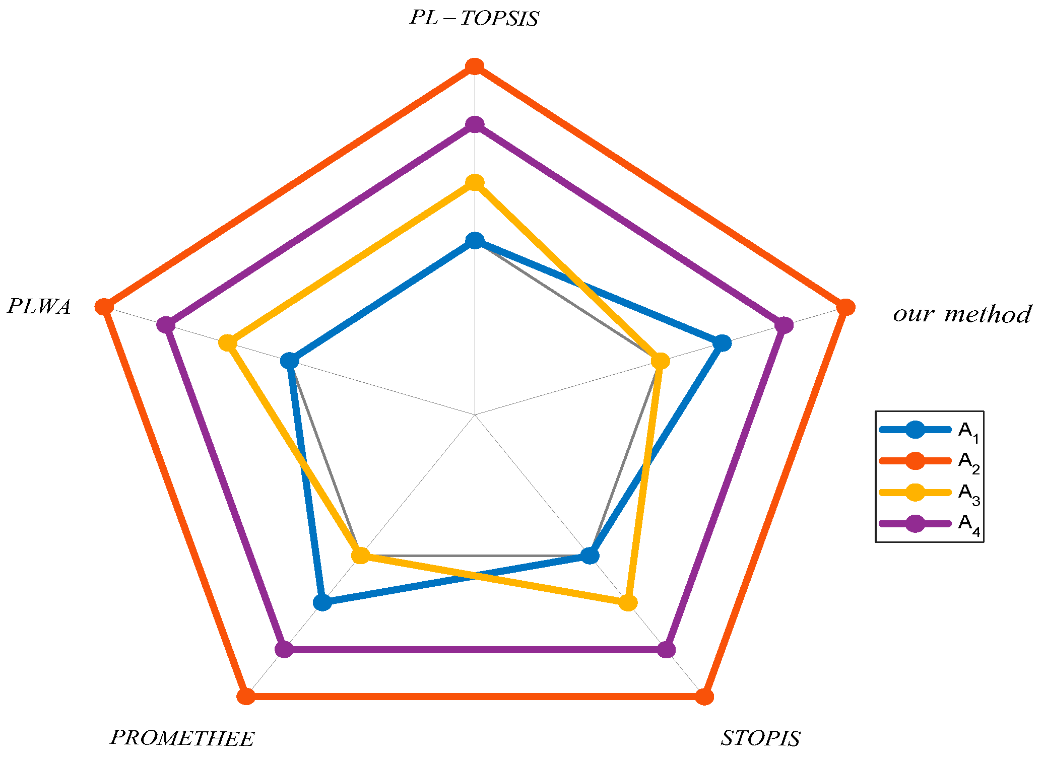
5.3. Visualization of Ranking Results

In order to better study the advantages of proposed algorithm, several algorithms have been compared and tested with it. The results are presented in Table 16 and Figure 3.
The proposed method ranked similarly with the PROMETHEE method. The PL-TOPSIS, SPOTIS, and PLWA method had comparable outcomes, differing one or two positions in accordance with the proposed method. All the ranking results yield the best results for A 2 and the second best for A 4 . WS Similarity Coefficient, which is sensitive to significant changes in ranking, is calculated by Equation (31). Additionally, RW Weighted Spearman’s Rank Correlation Coefficient, which permits the comparation of two vectors, is calculated by Equation (32).
W S = 1 2 x i x i y i max x i 1 , x i n
where n is ranking size and x i and y i are the values in the comparing rankings.
R W = 1 6 x i y i 2 n x i 1 + n y i 1 n n 3 + n 2 n 1
where the same elements in the Equation (31) are mentioned.
The WS and RW coefficients determined by the proposed methods are shown in Table 17. The results demonstrate that the PROMETHEE method ranked the proposed method equally. PL-TOPSIS, SPOTIS, and PLWA demonstrated a lesser degree of resemblance than PROMETHEE. Despite the disparities between the ranks, the correlation between their results and the similarity of our proposed method is substantial, ensuring a high degree of stability in the outcomes.

5.4. The Second Case Study

In order to illustrate the feasibility and validity of the proposed method better, a second case study is given. There are six attributes for shelter sites denoted as C 1 , C 2 , C 3 , C 4 , C 5 , and C 6 . Six sites are selected, denoted as A 1 , A 2 , A 3 , A 4 , A 5 , and A 6 . The computational and analytical processes are the same in Section 5.1.
Collect the experts’ evaluation towards the shelter sites selection (Table 18, Table 19 and Table 20).
According to the results of Table 18, Table 19 and Table 20 and Equation (24), the results are presented in Table 21.
Given the weights of all attributes ϖ 1 = 0.1 , ϖ 2 = 0.2 , ϖ 3 = 0.1 , ϖ 4 = 0.2 , ϖ 5 = 0.2 , ϖ 6 = 0.2 .
We get the dominance degree matrix, as follows:
ϑ ( A i , A e ) = 0 0.2341 0.6094 0.0077 0.2329 0.3654 0.5949 0 1.1027 0.5144 0.6257 0.7954 0.4412 0.0131 0 0.1938 0.07 0.0689 1.0686 0.569 1.1216 0 0.0027 0.94 0.9401 0.4755 1.2215 0.7807 0 1.0698 0.7855 0.3692 0.5622 0.2742 0.0061 0 .
Calculate the overall prospect value of each alternative A i ( i = 1 , 2 , 3 , 4 , 5 , 6 ) , and get:
δ ( A 1 ) = 0.9322 , δ ( A 2 ) = 0.4354 , δ ( A 3 ) = 0 = 1 , δ ( A 4 ) = 0.2378 , δ ( A 5 ) = 0 , δ ( A 6 ) = 0.5151 .
The ranking results of different methods are as follows, see Table 22.
All the ranking results yield the best results for A 3 , the second best for A 1 , and the third best for A 6 . The proposed method ranked similarly with other several methods when there are many attributes and alternatives.

6. Conclusions

The paper propsed a novel approach for MAGDM based on the new operational rules under PLTSs and the PLWDBMPA operator.
The innovations and advantages of this paper include the introduction of the TF-IDF keyword extraction technique as new weights, the definition of some new Dombi operations for PLTSs, and the PLDBMPA and PLWDBMPA operator on the basis of the proposed operational rules of PLTSs, which take into account the decision-makers’ subject preference and the relationship between the input arguments. Compared with the PL-TOPSIS, PLWA, SPOTIS, and PROMETHEE methods, the proposed method is demonstrated to be more scientific and accurate for the decision results derived from the case study, providing a more reasonable reference for experts to select the alternative shelter sites.
The proposed method in this paper also has some limitations. The PLWDBMPA operator cannot independently rank the alternatives; it still needs to be combined with some ranking methods like TOPSIS, VIKOR, and PROMETHEE. If there are too many alternatives and attributes, it might be quite flexible for Section 5.1. In terms of future research, we will improve the PLDBMPA and PLWDBMPA operators, making it rank the alternatives independently. We can also use Python, MATLAB to deal with the process of decision-making information fusion utilizing the PLWDBMPA operator. The Dombi operator can be applied to different fuzzy sets such as the intuitionistic fuzzy set, the q-rung orthopair fuzzy set, and the spherical fuzzy set. In addition, we also plan to extend our method to more scenarios, such as liquor brand evaluation, medical service, and emergency decision making.

Author Contributions

Conceptualization, J.W., X.Z. and S.L.; methodology, J.W. and X.Z.; software, X.Z.; validation, X.Z. and J.H.; formal analysis, J.W. and X.Z.; investigation, J.W.; resources, J.W. and J.H.; data curation, X.Z. and S.L.; writing-original draft preparation, X.Z.; writing-review and editing, J.W.; visualization, S.L.; supervision, J.W.; project administration, J.W. and J.H. All authors have read and agreed to the published version of the manuscript.

Funding

This study was funded by the Projects of Natural Science Research in Anhui Colleges and Universities (HYB20230132, KJ2021JD20, HYB20220179, 2023AH050178), the Projects of Natural Science Research in Anhui Jianzhu University (2021xskc01), the Research Program of Study Abroad for Outstanding Young Scholar in Universities of Anhui Province (gxgwfx2018074).

Data Availability Statement

The data of this study are available from the authors upon request.

Conflicts of Interest

The authors declare no conflict of interest.

Appendix A

Proof of Theorem 1.
L 1 ( P 1 ) L 2 ( P 2 ) = g 1 η 1 ( i ) g ( L 1 ) , η 2 ( j ) g ( L 2 ) 1 1 1 + η 1 ( i ) 1 η 1 ( i ) λ + η 2 ( j ) 1 η 2 ( j ) λ 1 / λ P 1 ( i ) P 2 ( j ) = g 1 η 1 ( i ) g ( L 1 ) , η 2 ( j ) g ( L 2 ) 1 1 1 + η 2 ( j ) 1 η 2 ( j ) λ + η 1 ( i ) 1 η 1 ( i ) λ 1 / λ P 2 ( j ) P 1 ( i ) = L 2 ( P 2 ) L 1 ( P 1 )
L 1 ( P 1 ) L 2 ( P 2 ) = g 1 η 1 ( i ) g ( L 1 ) , η 2 ( j ) g ( L 2 ) 1 1 + 1 η 1 ( i ) η 1 ( i ) λ + 1 η 2 ( j ) η 2 ( j ) λ 1 / λ P 1 ( i ) P 2 ( j ) = g 1 η 1 ( i ) g ( L 1 ) , η 2 ( j ) g ( L 2 ) 1 1 + 1 η 2 ( j ) η 2 ( j ) λ + 1 η 1 ( i ) η 1 ( i ) λ 1 / λ P 2 ( j ) P 1 ( i ) = L 2 ( P 2 ) L 1 ( P 1 ) .
δ L 1 ( P 1 ) L 2 ( P 2 ) = g 1 η 1 ( i ) g ( L 1 ) , η 2 ( j ) g ( L 2 ) 1 1 1 + δ η 1 ( i ) 1 η 1 ( i ) λ + η 2 ( j ) 1 η 2 ( j ) λ 1 / λ P 1 ( i ) P 2 ( j ) = g 1 η 1 ( i ) g ( L 1 ) , η 2 ( j ) g ( L 2 ) 1 1 1 + δ η 1 ( i ) 1 η 1 ( i ) λ + δ η 2 ( j ) 1 η 2 ( j ) λ 1 / λ P 1 ( i ) P 2 ( j ) = δ L 1 ( P 1 ) δ L 2 ( P 2 )
L 1 ( P 1 ) L 2 ( P 2 ) δ = g 1 η 1 ( i ) g ( L 1 ) , η 2 ( j ) g ( L 2 ) 1 1 + δ 1 η 1 ( i ) η 1 ( i ) λ + 1 η 2 ( j ) η 2 ( j ) λ 1 / λ P 1 ( i ) P 2 ( j ) = g 1 η 1 ( i ) g ( L 1 ) , η 2 ( j ) g ( L 2 ) 1 1 + δ 1 η 1 ( i ) η 1 ( i ) λ + δ 1 η 2 ( j ) η 2 ( j ) λ 1 / λ P 1 ( i ) P 2 ( j ) = L 1 ( P 1 ) δ L 2 ( P 2 ) δ
L ( P ) δ 1 L ( P ) δ 2 = g 1 η ( k ) g ( L ) 1 1 + δ 1 1 η ( k ) η ( k ) λ + δ 2 1 η ( k ) η ( k ) λ 1 / λ P ( k ) = g 1 η ( k ) g ( L ) 1 1 + ( δ 1 + δ 2 ) ( 1 η ( k ) η ( k ) ) λ 1 / λ P ( k ) = L ( P ) δ 1 + δ 2
 □

Appendix B

Proof of Theorem 2.
According to the operational rules of the PLTSs, we have
n ( 1 + T ( L i ( P i ) ) ) t = 1 n ( 1 + T ( L t ( P t ) ) ) L i ( P i ) = g 1 η i ( k ) g ( L i ) 1 1 1 + n ( 1 + T ( L i ( P i ) ) ) t = 1 n ( 1 + T ( L t ( P t ) ) ) η i ( k ) 1 η i ( k ) λ 1 / λ ( P i ( k ) ) n ( 1 + T ( L j ( P j ) ) ) t = 1 n ( 1 + T ( L t ( P t ) ) ) L j ( P j ) = g 1 η j ( d ) g ( L j ) 1 1 1 + n ( 1 + T ( L j ( P j ) ) ) t = 1 n ( 1 + T ( L t ( P t ) ) ) η j ( d ) 1 η j ( d ) λ 1 / λ ( P j ( d ) )
Let E i = n ( 1 + T ( L i ( P i ) ) ) t = 1 n ( 1 + T ( L t ( P t ) ) ) , E j = n ( 1 + T ( L j ( P j ) ) ) t = 1 n ( 1 + T ( L t ( P t ) ) ) , K i = 1 η i ( k ) η i ( k ) , D j = 1 η j ( d ) η j ( d ) .
Then,
n ( 1 + T ( L i ( P i ) ) ) t = 1 n ( 1 + T ( L t ( P t ) ) ) L i ( P i ) = g 1 η i ( k ) g ( L i ) 1 1 + E i 1 K i λ 1 / λ 1 ( P i ( k ) )
n ( 1 + T ( L j ( P j ) ) ) t = 1 n ( 1 + T ( L t ( P t ) ) ) L j ( P j ) = g 1 η j ( d ) g ( L j ) 1 1 + E j 1 D j λ 1 / λ 1 ( P j ( d ) )
n ( 1 + T ( L i ( P i ) ) ) t = 1 n ( 1 + T ( L t ( P t ) ) ) L i ( P i ) p = g 1 η i ( k ) g ( L i ) 1 + p E i 1 K i λ 1 / λ λ 1 / λ 1 ( P i ( k ) ) = g 1 η i ( k ) g ( L i ) 1 + p E i K i λ 1 / λ 1 ( P i ( k ) )
n ( 1 + T ( L j ( P j ) ) ) t = 1 n ( 1 + T ( L t ( P t ) ) ) L j ( P j ) q = g 1 η j ( d ) g ( L j ) 1 + q E j D j λ 1 / λ 1 ( P j ( d ) )
n ( 1 + T ( L i ( P i ) ) ) t = 1 n ( 1 + T ( L t ( P t ) ) ) L i ( P i ) p n ( 1 + T ( L j ( P j ) ) ) t = 1 n ( 1 + T ( L t ( P t ) ) ) L j ( P j ) q
= η i ( k ) g ( L i ) , η j ( d ) g ( L j ) g 1 1 1 + p E i K i λ 1 / λ λ + q E j D j λ 1 / λ λ 1 / λ P i ( k ) P j ( d ) = η i ( k ) g ( L i ) , η j ( d ) g ( L j ) g 1 1 1 + p E i K i λ + q E j D j λ 1 / λ P i ( k ) P j ( d )
i , j = 1 i j n n ( 1 + T ( L i ( P i ) ) ) t = 1 n ( 1 + T ( L t ( P t ) ) ) L i ( P i ) p n ( 1 + T ( L j ( P j ) ) ) t = 1 n ( 1 + T ( L t ( P t ) ) ) L j ( P j ) q
= η i ( k ) g ( L i ) , η j ( d ) g ( L j ) g 1 1 1 + i = 1 n j = 1 j i n p E i K i λ + q E j D j λ 1 1 / λ 1 Π i , j = 1 i j n P i ( k ) P j ( d )
= η i ( k ) g ( L i ) , η j ( d ) g ( L j ) g 1 1 1 + i = 1 n j = 1 j i n p E i K i λ + q E j D j λ 1 / λ λ 1 / λ 1 Π i , j = 1 i j n P i ( k ) P j ( d )
1 n ( n 1 ) i , j = 1 i j n n ( 1 + T ( L i ( P i ) ) ) t = 1 n ( 1 + T ( L t ( P t ) ) ) L i ( P i ) p n ( 1 + T ( L j ( P j ) ) ) t = 1 n ( 1 + T ( L t ( P t ) ) ) L j ( P j ) q = η i ( k ) g ( L i ) , η j ( d ) g ( L j ) g 1 1 1 + 1 n ( n 1 ) i = 1 n j = 1 j i n p E i K i λ + q E j D j λ 1 1 / λ λ 1 / λ 1 Π i , j = 1 i j n P i ( k ) P j ( d )
= η i ( k ) g ( L i ) , η j ( d ) g ( L j ) g 1 1 1 + 1 n ( n 1 ) i = 1 n j = 1 j i n p E i K i λ + q E j D j λ 1 1 / λ 1 Π i , j = 1 i j n P i ( k ) P j ( d )
1 n ( n 1 ) i , j = 1 i j n n ( 1 + T ( L i ( P i ) ) ) t = 1 n ( 1 + T ( L t ( P t ) ) ) L i ( P i ) p n ( 1 + T ( L j ( P j ) ) ) t = 1 n ( 1 + T ( L t ( P t ) ) ) L j ( P j ) q 1 p + q
= η i ( k ) g ( L i ) , η j ( d ) g ( L j ) g 1 1 + 1 p + q 1 n ( n 1 ) i = 1 n j = 1 j i n p E i K i λ + q E j D j λ 1 1 / λ λ 1 / λ 1 Π i , j = 1 i j n P i ( k ) P j ( d )
= η i ( k ) g ( L i ) , η j ( d ) g ( L j ) g 1 1 + n ( n 1 ) ( p + q ) i = 1 n j = 1 j i n p E i K i λ + q E j D j λ 1 1 1 / λ 1 Π i , j = 1 i j n P i ( k ) P j ( d )
 □

References

  1. Ahmad, N.; Hasan, M.G.; Barbhuiya, R.K. Identification and prioritization of strategies to tackle COVID-19 outbreak: A group-BWM based MCDM approach. Appl. Soft Comput. 2021, 111, 107642. [Google Scholar] [CrossRef] [PubMed]
  2. Lin, H.; You, J.; Xu, T. Evaluation of Online Teaching Quality: An Extended Linguistic MAGDM Framework Based on Risk Preferences and Unknown Weight Information. Symmetry 2021, 13, 192. [Google Scholar] [CrossRef]
  3. Han, Q.; Li, W.; Song, Y.; Zhang, T.; Wang, R. A New Method for MAGDM Based on Improved TOPSIS and a Novel Pythagorean Fuzzy Soft Entropy. Symmetry 2019, 11, 905. [Google Scholar] [CrossRef]
  4. Peng, Y.; Tao, Y.; Wu, B.; Wang, X. Probabilistic Hesitant Intuitionistic Fuzzy Linguistic Term Sets and Their Application in Multiple Attribute Group Decision Making. Symmetry 2020, 12, 1932. [Google Scholar] [CrossRef]
  5. Wang, J.-X. A MAGDM Algorithm with Multi-Granular Probabilistic Linguistic Information. Symmetry 2019, 11, 127. [Google Scholar] [CrossRef]
  6. Wang, J.; Li, S.; Zhou, X. A Novel GDMD-PROMETHEE Algorithm Based on the Maximizing Deviation Method and Social Media Data Mining for Large Group Decision Making. Symmetry 2023, 15, 387. [Google Scholar] [CrossRef]
  7. Yan, L. EDAS-aided intelligent decision-making in interior decoration design quality assessment using 2-tuple linguistic pythagorean fuzzy sets. Int. J. Knowl.-Based Intell. Eng. Systems. 2023, 1–16, preprint. [Google Scholar] [CrossRef]
  8. Ziemba, P. Energy Security Assessment Based on a New Dynamic Multi-Criteria Decision-Making Framework. Energies 2022, 15, 9356. [Google Scholar] [CrossRef]
  9. Ahmad, Q.S.; Khan, M.F.; Ahmad, N. Multi-Criteria Group Decision-Making Models in a Multi-Choice Environment. Axioms 2022, 11, 659. [Google Scholar] [CrossRef]
  10. Stević, Ž.; Zavadskas, E.K.; Tawfiq, F.M.O.; Tchier, F.; Davidov, T. Fuzzy Multicriteria Decision-Making Model Based on Z Numbers for the Evaluation of Information Technology for Order Picking in Warehouses. Appl. Sci. 2022, 12, 12533. [Google Scholar] [CrossRef]
  11. Dombi, J. A general class of fuzzy operators, the demorgan class of fuzzy operators and fuzziness measures induced by fuzzy operators. Fuzzy Sets Syst. 1982, 8, 149–163. [Google Scholar] [CrossRef]
  12. Liu, P.; Liu, J.; Chen, S.-M. Some intuitionistic fuzzy Dombi Bonferroni mean operators and their application to multi-attribute group decision making. J. Oper. Res. Society. 2018, 69, 1–24. [Google Scholar] [CrossRef]
  13. He, X. Typhoon disaster assessment based on Dombi hesitant fuzzy information aggregation operators. Nat. Hazards. 2018, 90, 1153–1175. [Google Scholar] [CrossRef]
  14. Bonferroni, C. Sulle medie multiple di potenze. Boll. Mat. Ital. 1950, 5, 267–270. [Google Scholar]
  15. Xu, Z.; Yager, R.R. Some geometric aggregation operators based on intuitionistic fuzzy sets. Int. J. Gen. Systems. 2006, 35, 417–433. [Google Scholar] [CrossRef]
  16. Liang, D.; Kobina, A.; Quan, W. Grey Relational Analysis Method for Probabilistic Linguistic Multi-criteria Group Decision-Making Based on Geometric Bonferroni Mean. Int. J. Fuzzy Systems. 2018, 20, 2234–2244. [Google Scholar] [CrossRef]
  17. Zhu, B.; Xu, Z.S. Hesitant fuzzy Bonferroni means for multi-criteria decision making. J. Oper. Res. Society. 2013, 64, 1831–1840. [Google Scholar] [CrossRef]
  18. Liu, P. Multi-attribute decision-making method research based on interval vague set and TOPSIS method. Ūkio Technol. Ekon. Vystym. 2009, 15, 453–463. [Google Scholar] [CrossRef]
  19. Yue, Z. An extended TOPSIS for determining weights of decision makers with interval numbers. Knowl Based Syst. 2011, 24, 146–153. [Google Scholar] [CrossRef]
  20. Opricovic, S.; Tzeng, G.-H. Compromise solution by MCDM methods: A comparative analysis of VIKOR and TOPSIS. Eur. J. Oper. Res. 2004, 156, 445–455. [Google Scholar] [CrossRef]
  21. Ren, Z.; Xu, Z.; Wang, H. Dual hesitant fuzzy VIKOR method for multi-criteria group decision making based on fuzzy measure and new comparison method. Inf. Sci. 2017, 388–389, 1–16. [Google Scholar] [CrossRef]
  22. Liu, P.; Zhang, X. Research on the supplier selection of a supply chain based on entropy weight and improved ELECTRE-III method. Int. J. Prod. Res. 2011, 49, 637–646. [Google Scholar] [CrossRef]
  23. Akram, M.; Luqman, A.; Kahraman, C. Hesitant Pythagorean fuzzy ELECTRE-II method for multi-criteria decision-making problems. Appl. Soft Comput. 2021, 108, 107479. [Google Scholar] [CrossRef]
  24. Krishankumar, R.; Ravichandran, K.S.; Saeid, A.B. A new extension to PROMETHEE under intuitionistic fuzzy environment for solving supplier selection problem with linguistic preferences. Appl. Soft Comput. 2017, 60, 564–576. [Google Scholar] [CrossRef]
  25. Akram, M.; Noreen, U.; Pamucar, D. Extended PROMETHEE approach with 2-tuple linguistic m-polar fuzzy sets for selection of elliptical cardio machine. Expert Systems. 2023, 40, e13178. [Google Scholar] [CrossRef]
  26. Li, P.; Xu, Z.; Wei, C.; Bai, Q.; Liu, J. A novel PROMETHEE method based on GRA-DEMATEL for PLTSs and its application in selecting renewable energies. Inf. Sci. 2022, 589, 142–161. [Google Scholar] [CrossRef]
  27. Wang, X.; Li, Y.; Xu, Z.; Luo, Y. Nested information representation of multi-dimensional decision: An improved PROMETHEE method based on NPLTSs. Inf. Sci. 2022, 607, 1224–1244. [Google Scholar] [CrossRef]
  28. Dezert, J.; Tchamova, A.; Han, D.; Tacnet, J.-M. The SPOTIS rank reversal free method for multi-criteria decision-making support. In Proceedings of the 2020 IEEE 23rd International Conference on Information Fusion (FUSION), Rustenburg, South Africa, 6–9 July 2020; pp. 1–8. [Google Scholar]
  29. Więckowski, J.; Król, R.; Wątróbski, J. Towards robust results in Multi-Criteria Decision Analysis: Ranking reversal free methods case study. Procedia Comput. Science 2022, 207, 4584–4592. [Google Scholar] [CrossRef]
  30. Sałabun, W.; Piegat, A.; Wątróbski, J.; Karczmarczyk, A.; Jankowski, J. The COMET method: The first MCDA method completely resistant to rank reversal paradox. Eur. Work. Group Series. 2019, 3, 10–16. [Google Scholar]
  31. Stoilova, S.; Munier, N. A Novel Fuzzy SIMUS Multicriteria Decision-Making Method. An Application in Railway Passenger Transport Planning. Symmetry. 2021, 13, 483. [Google Scholar] [CrossRef]
  32. Wątróbski, J.; Bączkiewicz, A.; Ziemba, E.; Sałabun, W. Sustainable cities and communities assessment using the DARIA-TOPSIS method. Sustain. Cities Society 2022, 83, 103926. [Google Scholar] [CrossRef]
  33. Gomes, L.; Lima, M. TODIMI: Basics and application to multicriteria ranking. Found. Comput. Decis. Sci. 1991, 16, 1–16. [Google Scholar]
  34. Liu, Y.; Bao, T.; Zhao, D.; Sang, H.; Fu, B. Evaluation of Student-Perceived Service Quality in Higher Education for Sustainable Development: A Fuzzy TODIM-ERA Method. Sustainability 2022, 14, 4761. [Google Scholar] [CrossRef]
  35. Liu, Y.-H.; Peng, H.-M.; Wang, T.-L.; Wang, X.-K.; Wang, J.-Q. Supplier Selection in the Nuclear Power Industry with an Integrated ANP-TODIM Method under Z-Number Circumstances. Symmetry 2020, 12, 1357. [Google Scholar] [CrossRef]
  36. Xiao, F. Method for classroom teaching quality evaluation in college English based on the probabilistic uncertain linguistic multiple-attribute group decision-making. Int. J. Knowl. Based Intell. Eng. Systems 2023, 1, 1–13, preprint. [Google Scholar] [CrossRef]
  37. He, X.; Wu, J.; Wang, C.; Ye, M. Historical Earthquakes and Their Socioeconomic Consequences in China: 1950–2017. Int. J. Environ. Res. Public Health 2018, 15, 2728. [Google Scholar] [CrossRef] [PubMed]
  38. Zhao, J.; Ding, F.; Wang, Z.; Ren, J.; Zhao, J.; Wang, Y.; Tang, X.; Wang, Y.; Yao, J.; Li, Q. A Rapid Public Health Needs Assessment Framework for after Major Earthquakes Using High-Resolution Satellite Imagery. Int. J. Environ. Res. Public Health 2018, 15, 1111. [Google Scholar] [CrossRef] [PubMed]
  39. Trivedi, A. A multi-criteria decision approach based on DEMATEL to assess determinants of shelter site selection in disaster response. Int. J. Disaster Risk Reduct. 2018, 31, 722–728. [Google Scholar] [CrossRef]
  40. Xu, Y.; Wen, X.; Zhang, W. A two-stage consensus method for large-scale multi-attribute group decision making with an application to earthquake shelter selection. Comput. Ind. Eng. 2018, 116, 113–129. [Google Scholar] [CrossRef]
  41. Song, S.; Zhou, H.; Song, W. Sustainable shelter-site selection under uncertainty: A rough QUALIFLEX method. Comput. Ind. Eng. 2019, 128, 371–386. [Google Scholar] [CrossRef]
  42. Zhang, W.; Yoshida, T.; Tang, X. A comparative study of TF*IDF, LSI and multi-words for text classification. Expert Syst. Appl. 2011, 38, 2758–2765. [Google Scholar] [CrossRef]
  43. Pang, Q.; Wang, H.; Xu, Z. Probabilistic linguistic term sets in multi-attribute group decision making. Inf. Sci. 2016, 369, 128–143. [Google Scholar] [CrossRef]
  44. Gou, X.; Xu, Z. Novel basic operational laws for linguistic terms, hesitant fuzzy linguistic term sets and probabilistic linguistic term sets. Inf. Sci. 2016, 372, 407–427. [Google Scholar] [CrossRef]
  45. Yager, R.R. The power average operator. IEEE Trans. Syst. Man Cybern. Part A Syst. Humans 2001, 31, 724–731. [Google Scholar] [CrossRef]
Figure 1. Flowchart of the decision procedure.
Symmetry 15 01807 g001
Figure 2. “2.6” Turkey Earthquake word cloud map.
Symmetry 15 01807 g002
Figure 3. Radar chart of the ranking results.
Symmetry 15 01807 g003
Table 1. The probabilistic linguistic decision matrix D 1 provided by the expert e 1 .
e 1 C 1 C 2 C 3
A 1 s 1 ( 1 ) s 2 ( 1 ) s 0 ( 1 )
A 2 s 2 ( 1 ) s 1 ( 0.5 ) , s 2 ( 0.5 ) s 0 ( 0.2 ) , s 1 ( 0.4 ) , s 2 ( 0.4 )
A 3 s 1 ( 1 ) s 0 ( 1 ) s 1 ( 0.6 ) , s 2 ( 0.4 )
A 4 s 1 ( 0.5 ) , s 2 ( 0.5 ) s 0 ( 0.4 ) , s 1 ( 0.6 ) s 1 ( 1 )
Table 2. The probabilistic linguistic decision matrix D 2 provided by the expert e 2 .
e 2 C 1 C 2 C 3
A 1 s 0 ( 0.4 ) , s 1 ( 0.6 ) s 1 ( 0.5 ) , s 2 ( 0.5 ) s 2 ( 0.2 ) , s 1 ( 0.4 ) , s 0 ( 0.4 )
A 2 s 0 ( 0.3 ) , s 1 ( 0.3 ) , s 2 ( 0.4 ) s 0 ( 1 ) s 2 ( 1 )
A 3 s 0 ( 1 ) s 1 ( 1 ) s 2 ( 1 )
A 4 s 1 ( 1 ) s 1 ( 1 ) s 0 ( 0.1 ) , s 1 ( 0.9 )
Table 3. The probabilistic linguistic decision matrix D 3 provided by the expert e 3 .
e 3 C 1 C 2 C 3
A 1 s 1 ( 1 ) s 2 ( 1 ) s 0 ( 1 )
A 2 s 2 ( 1 ) s 0 ( 1 ) s 2 ( 1 )
A 3 s 1 ( 0.8 ) , s 2 ( 0.2 ) s 1 ( 0.7 ) , s 2 ( 0.3 ) s 2 ( 1 )
A 4 s 2 ( 1 ) s 1 ( 1 ) s 1 ( 1 )
Table 4. The deviation degree between PLTSs based on matrices D 1 , D 2 , and D 3 according to attribute C 1 .
i d ( L i 1 1 ( P i 1 1 ) , L i 1 2 ( P i 1 2 ) ) d ( L i 1 1 ( P i 1 1 ) , L i 1 3 ( P i 1 3 ) ) d ( L i 1 2 ( P i 1 2 ) , L i 1 3 ( P i 1 3 ) )
10.192500.1925
20.322700.3227
30.09620.12320.0981
40.24060.30810.0962
Table 5. The deviation degree between PLTSs based on matrices D 1 , D 2 , and D 3 according to attribute C 2 .
i d ( L i 2 1 ( P i 2 1 ) , L i 2 2 ( P i 2 2 ) ) d ( L i 2 1 ( P i 2 1 ) , L i 2 3 ( P i 2 3 ) ) d ( L i 2 2 ( P i 2 2 ) , L i 2 3 ( P i 2 3 ) )
10.308100.3081
20.19840.19840
30.09620.14560.1848
40.19250.19250
Table 6. The deviation degree between PLTSs based on matrices D 1 , D 2 , and D 3 according to attribute C 3 .
i d ( L i 3 1 ( P i 3 1 ) , L i 3 2 ( P i 3 2 ) ) d ( L i 3 1 ( P i 3 1 ) , L i 3 3 ( P i 3 3 ) ) d ( L i 3 2 ( P i 3 2 ) , L i 3 3 ( P i 3 3 ) )
10.190500.1905
20.33220.33220
30.31560.31560
40.048100.0481
Table 7. The support degree between PLTSs based on matrices D 1 , D 2 , and D 3 according to attribute C 1 .
i sup ( L i 1 1 ( P i 1 1 ) , L i 1 2 ( P i 1 2 ) ) sup ( L i 1 1 ( P i 1 1 ) , L i 1 3 ( P i 1 3 ) ) sup ( L i 1 2 ( P i 1 2 ) , L i 1 3 ( P i 1 3 ) )
10.510.5
20.510.5
30.69700.61200.6910
40.62700.52230.8508
Table 8. The support degree between PLTSs based on matrices D 1 , D 2 , and D 3 according to attribute C 2 .
i sup ( L i 2 1 ( P i 2 1 ) , L i 2 2 ( P i 2 2 ) ) sup ( L i 2 1 ( P i 2 1 ) , L i 2 3 ( P i 2 3 ) ) sup ( L i 2 2 ( P i 2 2 ) , L i 2 3 ( P i 2 3 ) )
10.510.5
20.50.51
30.77450.65870.5668
40.50.51
Table 9. The support degree between PLTSs based on matrices D 1 , D 2 , and D 3 according to attribute C 3 .
i sup ( L i 3 1 ( P i 3 1 ) , L i 3 2 ( P i 3 2 ) ) sup ( L i 3 1 ( P i 3 1 ) , L i 3 3 ( P i 3 3 ) ) sup ( L i 3 2 ( P i 3 2 ) , L i 3 3 ( P i 3 3 ) )
10.510.5
20.50.51
30.50.51
40.510.5
Table 10. The integrated probabilistic linguistic decision matrix D .
C 1 C 2 C 3
A 1 s 0.6338 ( 0.0256 ) , s 0.8252 ( 0.0576 ) , s 0.8482 ( 0.0576 ) , s 0.9889 ( 0.1296 ) s 1.6921 ( 0.0625 ) , s 1.8650 ( 0.0625 ) , s 1.8824 ( 0.0625 ) , s 1.9930 ( 0.0625 ) s 0.6767 ( 0.0016 ) , s 0.5259 ( 0.0064 ) , s 0.5199 ( 0.0064 ) , s 0.3940 ( 0.0256 ) , s 0.2924 ( 0.0064 ) , s 0.2599 ( 0.0064 ) , s 0.1924 ( 0.0256 ) , s 0.1676 ( 0.0256 ) , s 0.0125 ( 0.0256 )
A 2 s 1.5575 ( 0.0081 ) , s 1.6292 ( 0.0081 ) , s 1.6313 ( 0.0081 ) , s 1.6921 ( 0.0081 ) , s 1.8263 ( 0.0144 ) , s 1.8468 ( 0.0144 ) , s 1.8650 ( 0.0144 ) , s 1.8824 ( 0.0144 ) , s 1.9930 ( 0.0256 ) s 0.2745 ( 0.0625 ) , s 0.3313 ( 0.0625 ) , s 0.3560 ( 0.0625 ) , s 0.4068 ( 0.0625 ) s 1.5575 ( 0.0016 ) , s 1.6292 ( 0.0064 ) , s 1.6313 ( 0.0064 ) , s 1.6921 ( 0.0256 ) , s 1.8263 ( 0.0064 ) , s 1.8468 ( 0.0064 ) , s 1.8650 ( 0.0256 ) , s 1.8824 ( 0.0256 ) , s 1.9930 ( 0.0256 )
A 3 s 0.6373 ( 0.4096 ) , s 0.6623 ( 0.0256 ) , s 0.8412 ( 0.0256 ) , s 0.8593 ( 0.0016 ) s 0.6388 ( 0.2401 ) , s 0.6644 ( 0.0441 ) , s 0.8450 ( 0.0441 ) , s 0.8635 ( 0.0081 ) s 1.6921 ( 0.1296 ) , s 1.8650 ( 0.0576 ) , s 1.8824 ( 0.0576 ) , s 1.9930 ( 0.0256 )
A 4 s 1.2113 ( 0.0625 ) , s 1.3090 ( 0.0625 ) , s 1.6474 ( 0.0625 ) , s 1.6875 ( 0.0625 ) s 0.6338 ( 0.0256 ) , s 0.8252 ( 0.0576 ) , s 0.8482 ( 0.0576 ) , s 0.9889 ( 0.1296 ) s 0.6338 ( 0.0001 ) , s 0.8252 ( 0.0081 ) , s 0.8482 ( 0.0081 ) , s 0.9889 ( 0.6561 )
Table 11. Attributes and their corresponding keywords.
AttributeKeywords IncludedNumber of Terms ϖ j
Scale and locationContractor, building, campsite, city, etc.80.2581
AccessibilitySecurity, aftershock, safeguard, hospital, etc.130.4193
Resource availabilitySupplies, assistance, container, contribution, etc.100.3226
Table 12. The probabilistic linguistic decision matrix.
C 1 C 2 C 3
A 1 s 1 ( 0.87 ) , s 0 ( 0.13 ) s 2 ( 0.83 ) , s 1 ( 0.17 ) s 0 ( 0.8 ) , s 1 ( 0.13 ) , s 2 ( 0.07 )
A 2 s 2 ( 0.8 ) , s 1 ( 0.1 ) , s 0 ( 0.1 ) s 1 ( 0.5 ) , s 2 ( 0.5 ) s 2 ( 0.8 ) , s 1 ( 0.13 ) , s 0 ( 0.07 )
A 3 s 1 ( 0.6 ) , s 0 ( 0.4 ) s 2 ( 0.1 ) , s 1 ( 0.57 ) , s 0 ( 0.33 ) s 1 ( 0.2 ) , s 2 ( 0.8 )
A 4 s 1 ( 0.5 ) , s 2 ( 0.5 ) s 1 ( 0.87 ) , s 0 ( 0.13 ) s 1 ( 0.97 ) , s 0 ( 0.03 )
Table 13. The dominance degree of the six cars.
A 1 A 2 A 3 A 4
A 1 0.5000 0.2543 0.5482 0.4180
A 2 0.7457 0.5000 0.8460 0.7476
A 3 0.4518 0.1540 0.5000 0.3268
A 4 0.5820 0.2524 0.6732 0.5000
Table 14. The relative dominance degree among the six cars.
Φ + ( A i ) Φ ( A i ) Φ ( A i )
A 1 0.4301 0.5699 −0.1398
A 2 0.7098 0.2902 0.4197
A 3 0.3582 0.6418 −0.2836
A 4 0.5019 0.4981 0.0038
Table 15. The probabilistic linguistic generated decision matrix.
C 1 C 2 C 3
A 1 0.6450.8050.455
A 2 0.7830.7500.788
A 3 0.6000.6280.800
A 4 0.7500.6450.662
Weights0.30.30.4
TypesProfitProfitProfit
Table 16. Ranking results of different methods.
A 1 A 2 A 3 A 4 Rank
Our Method0.27991.00000.00000.5733 A 2 A 4 A 1 A 3
PL-TOPSIS−0.60000.0000−0.4920−0.2880 A 2 A 4 A 3 A 1
PLWA0.21690.25700.22550.2258 A 2 A 4 A 3 A 1
PROMETHEE−0.13980.4197−0.28360.0038 A 2 A 4 A 1 A 3
SPOTIS0.62640.10690.60000.4866 A 2 A 4 A 3 A 1
Table 17. Correlations with reference ranking of proposed methods.
CoefficientPL-TOPSISPLWAPROMETHEESPOTIS
WS0.9170.9171.0000.917
RW0.7400.7401.0000.740
Table 18. The probabilistic linguistic decision matrix D 1 provided by the expert e 1 .
e 1 C 1 C 2 C 3
A 1 s 1 ( 1 ) s 2 ( 1 ) s 0 ( 1 )
A 2 s 2 ( 1 ) s 1 ( 0.5 ) , s 2 ( 0.5 ) s 0 ( 0.2 ) , s 1 ( 0.4 ) , s 2 ( 0.4 )
A 3 s 1 ( 0.5 ) , s 2 ( 0.5 ) s 1 ( 1 ) s 0 ( 0.1 ) , s 1 ( 0.9 )
A 4 s 1 ( 1 ) s 0 ( 1 ) s 1 ( 0.6 ) , s 2 ( 0.4 )
A 5 s 0 ( 1 ) s 0 ( 1 ) s 2 ( 1 )
A 6 s 1 ( 0.5 ) , s 2 ( 0.5 ) s 0 ( 0.4 ) , s 1 ( 0.6 ) s 1 ( 1 )
e 1 C 4 C 5 C 6
A 1 s 2 ( 1 ) s 0 ( 1 ) s 1 ( 1 )
A 2 s 1 ( 1 ) s 1 ( 0.5 ) , s 2 ( 0.5 ) s 0 ( 1 )
A 3 s 0 ( 0.3 ) , s 1 ( 0.3 ) , s 2 ( 0.4 ) s 1 ( 1 ) s 0 ( 0.1 ) , s 1 ( 0.9 )
A 4 s 0 ( 1 ) s 0 ( 1 ) s 1 ( 0.6 ) , s 2 ( 0.4 )
A 5 s 0 ( 1 ) s 0 ( 1 ) s 2 ( 1 )
A 6 s 1 ( 0.5 ) , s 2 ( 0.5 ) s 0 ( 0.4 ) , s 1 ( 0.6 ) s 1 ( 1 )
Table 19. The probabilistic linguistic decision matrix D 2 provided by the expert e 2 .
e 2 C 1 C 2 C 3
A 1 s 0 ( 0.4 ) , s 1 ( 0.6 ) s 1 ( 0.5 ) , s 2 ( 0.5 ) s 2 ( 0.2 ) , s 1 ( 0.4 ) , s 0 ( 0.4 )
A 2 s 0 ( 0.3 ) , s 1 ( 0.3 ) , s 2 ( 0.4 ) s 0 ( 1 ) s 2 ( 1 )
A 3 s 2 ( 1 ) s 2 ( 1 ) s 1 ( 1 )
A 4 s 0 ( 1 ) s 1 ( 1 ) s 2 ( 1 )
A 5 s 0 ( 0.3 ) , s 2 ( 0.7 ) s 1 ( 0.2 ) , s 2 ( 0.8 ) s 2 ( 1 )
A 6 s 1 ( 1 ) s 1 ( 1 ) s 0 ( 0.1 ) , s 1 ( 0.9 )
e 2 C 4 C 5 C 6
A 1 s 1 ( 0.6 ) , s 2 ( 0.4 ) s 1 ( 0.5 ) , s 2 ( 0.5 ) s 1 ( 0.6 ) , s 2 ( 0.4 )
A 2 s 0 ( 1 ) s 0 ( 1 ) s 1 ( 1 )
A 3 s 1 ( 1 ) s 2 ( 1 ) s 1 ( 1 )
A 4 s 0 ( 1 ) s 1 ( 1 ) s 2 ( 1 )
A 5 s 0 ( 0.3 ) , s 2 ( 0.7 ) s 1 ( 0.2 ) , s 2 ( 0.8 ) s 2 ( 1 )
A 6 s 1 ( 1 ) s 1 ( 1 ) s 0 ( 0.1 ) , s 1 ( 0.9 )
Table 20. The probabilistic linguistic decision matrix D 3 provided by the expert e 3 .
e 3 C 1 C 2 C 3
A 1 s 1 ( 1 ) s 2 ( 1 ) s 0 ( 1 )
A 2 s 2 ( 1 ) s 0 ( 1 ) s 2 ( 1 )
A 3 s 2 ( 1 ) s 1 ( 0.5 ) , s 2 ( 0.5 ) s 1 ( 1 )
A 4 s 1 ( 0.8 ) , s 2 ( 0.2 ) s 1 ( 0.7 ) , s 2 ( 0.3 ) s 2 ( 1 )
A 5 s 1 ( 1 ) s 0 ( 1 ) s 1 ( 0.7 ) , s 2 ( 0.3 )
A 6 s 2 ( 1 ) s 1 ( 1 ) s 1 ( 1 )
e 3 C 4 C 5 C 6
A 1 s 2 ( 1 ) s 2 ( 1 ) s 2 ( 1 )
A 2 s 0 ( 0.3 ) , s 2 ( 0.7 ) s 0 ( 1 ) s 2 ( 1 )
A 3 s 1 ( 1 ) s 1 ( 0.5 ) , s 2 ( 0.5 ) s 2 ( 1 )
A 4 s 1 ( 0.2 ) , s 2 ( 0.8 ) s 1 ( 0.7 ) , s 2 ( 0.3 ) s 2 ( 1 )
A 5 s 1 ( 1 ) s 0 ( 1 ) s 1 ( 0.7 ) , s 2 ( 0.3 )
A 6 s 2 ( 1 ) s 1 ( 1 ) s 1 ( 1 )
Table 21. The integrated probabilistic linguistic decision matrix D .
C 1 C 2 C 3
A 1 s 0.6338 ( 0.0256 ) , s 0.8252 ( 0.0576 ) , s 0.8482 ( 0.0576 ) , s 0.9889 ( 0.1296 ) s 1.6921 ( 0.0625 ) , s 1.8650 ( 0.0625 ) , s 1.8824 ( 0.0625 ) , s 1.9930 ( 0.0625 ) s 0.6767 ( 0.0016 ) , s 0.5259 ( 0.0064 ) , s 0.5199 ( 0.0064 ) , s 0.3940 ( 0.0256 ) , s 0.2924 ( 0.0064 ) , s 0.2599 ( 0.0064 ) , s 0.1924 ( 0.0256 ) , s 0.1676 ( 0.0256 ) , s 0.0125 ( 0.0256 )
A 2 s 1.5575 ( 0.0081 ) , s 1.6292 ( 0.0081 ) , s 1.6313 ( 0.0081 ) , s 1.6921 ( 0.0081 ) , s 1.8263 ( 0.0144 ) , s 1.8468 ( 0.0144 ) , s 1.8650 ( 0.0144 ) , s 1.8824 ( 0.0144 ) , s 1.9930 ( 0.0256 ) s 0.2745 ( 0.0625 ) , s 0.3313 ( 0.0625 ) , s 0.3560 ( 0.0625 ) , s 0.4068 ( 0.0625 ) s 1.5575 ( 0.0016 ) , s 1.6292 ( 0.0064 ) , s 1.6313 ( 0.0064 ) , s 1.6921 ( 0.0256 ) , s 1.8263 ( 0.0064 ) , s 1.8468 ( 0.0064 ) , s 1.8650 ( 0.0256 ) , s 1.8824 ( 0.0256 ) , s 1.9930 ( 0.0256 )
A 3 s 1.6921 ( 0.0625 ) , s 1.8650 ( 0.0625 ) , s 1.8824 ( 0.0625 ) , s 1.9930 ( 0.0625 ) s 1.2113 ( 0.0625 ) , s 1.3090 ( 0.0625 ) , s 1.6474 ( 0.0625 ) , s 1.6875 ( 0.0625 ) s 0.6338 ( 0.0001 ) , s 0.8252 ( 0.0081 ) , s 0.8482 ( 0.0081 ) , s 0.9889 ( 0.6561 )
A 4 s 0.6373 ( 0.4096 ) , s 0.6623 ( 0.0256 ) , s 0.8412 ( 0.0256 ) , s 0.8593 ( 0.0016 ) s 0.6388 ( 0.2401 ) , s 0.6644 ( 0.0441 ) , s 0.8450 ( 0.0441 ) , s 0.8635 ( 0.0081 ) s 1.6921 ( 0.1296 ) , s 1.8650 ( 0.0576 ) , s 1.8824 ( 0.0576 ) , s 1.9930 ( 0.0256 )
A 5 s 0.2117 ( 0.0081 ) , s 0.3553 ( 0.0441 ) , s 0.8906 ( 0.0441 ) , s 0.9449 ( 0.2401 ) s 0.2745 ( 0.0016 ) , s 0.3313 ( 0.0256 ) , s 0.3560 ( 0.0256 ) , s 0.4068 ( 0.4096 ) s 1.6921 ( 0.2401 ) , s 1.8650 ( 0.0441 ) , s 1.8824 ( 0.0441 ) , s 1.9930 ( 0.0081 )
A 6 s 1.2113 ( 0.0625 ) , s 1.3090 ( 0.0625 ) , s 1.6474 ( 0.0625 ) , s 1.6875 ( 0.0625 ) s 0.6338 ( 0.0256 ) , s 0.8252 ( 0.0576 ) , s 0.8482 ( 0.0576 ) , s 0.9889 ( 0.1296 ) s 0.6338 ( 0.0001 ) , s 0.8252 ( 0.0081 ) , s 0.8482 ( 0.0081 ) , s 0.9889 ( 0.6561 )
C 4 C 5 C 6
A 1 s 1.6921 ( 0.1296 ) , s 1.8650 ( 0.0576 ) , s 1.8824 ( 0.0576 ) , s 1.9930 ( 0.0256 ) s 0.8577 ( 0.0625 ) , s 0.8796 ( 0.0625 ) , s 1.5330 ( 0.0625 ) , s 1.5390 ( 0.0625 ) s 1.2163 ( 0.1296 ) , s 1.3109 ( 0.0576 ) , s 1.6511 ( 0.0576 ) , s 1.6899 ( 0.0256 )
A 2 s 0.2117 ( 0.0081 ) , s 0.3553 ( 0.0441 ) , s 0.8906 ( 0.0441 ) , s 9449 ( 0.2401 ) s 0.2745 ( 0.0625 ) , s 0.3313 ( 0.0625 ) , s 0.3560 ( 0.0625 ) , s 0.4068 ( 0.0625 ) s 0.6388 ( 0.2401 ) , s 0.6644 ( 0.0441 ) , s 0.8450 ( 0.0441 ) , s 0.8635 ( 0.0081 )
A 3 s 0.6338 ( 0.0081 ) , s 0.8252 ( 0.0081 ) , s 0.8482 ( 0.0081 ) , s 0.9889 ( 0.0081 ) , s 1.0110 ( 0.0144 ) , s 1.0757 ( 0.0144 ) , s 1.1339 ( 0.0144 ) , s 1.1736 ( 0.0144 ) , s 1.2803 ( 0.0256 ) s 1.2113 ( 0.0625 ) , s 1.3090 ( 0.0625 ) , s 1.6474 ( 0.0625 ) , s 1.6875 ( 0.0625 ) s 0.8738 ( 0.0001 ) , s 1.0118 ( 0.0081 ) , s 1.1315 ( 0.0081 ) , s 1.2223 ( 0.6561 )
A 4 s 0.2745 ( 0.0016 ) , s 0.3313 ( 0.0256 ) , s 0.3560 ( 0.0256 ) , s 0.4068 ( 0.4096 ) s 0.6388 ( 0.2401 ) , s 0.6644 ( 0.0441 ) , s 0.8450 ( 0.0441 ) , s 0.8635 ( 0.0081 ) s 1.6921 ( 0.1296 ) , s 1.8650 ( 0.0576 ) , s 1.8824 ( 0.0576 ) , s 1.9930 ( 0.0256 )
A 5 s 0.2117 ( 0.0081 ) , s 0.3553 ( 0.0441 ) , s 0.8906 ( 0.0441 ) , s 9449 ( 0.2401 ) s 0.2745 ( 0.0016 ) , s 0.3313 ( 0.0256 ) , s 0.3560 ( 0.0256 ) , s 0.4068 ( 0.4096 ) s 1.6921 ( 0.2401 ) , s 1.8650 ( 0.0441 ) , s 1.8824 ( 0.0441 ) , s 1.9930 ( 0.0081 )
A 6 s 1.2113 ( 0.0625 ) , s 1.3090 ( 0.0625 ) , s 1.6474 ( 0.0625 ) , s 1.6875 ( 0.0625 ) s 0.6338 ( 0.0256 ) , s 0.8252 ( 0.0576 ) , s 0.8482 ( 0.0576 ) , s 0.9889 ( 0.1296 ) s 0.6338 ( 0.0001 ) , s 0.8252 ( 0.0081 ) , s 0.8482 ( 0.0081 ) , s 0.9889 ( 0.6561 )
Table 22. Ranking results of different methods.
A 1 A 2 A 3 A 4 A 5 A 6 Rank
Our Method0.93320.43541.00000.23780.00000.5151 A 3 A 1 A 6 A 2 A 4 A 5
PL-TOPSIS−0.1223−0.58920.0000−0.5169−0.5568−0.1505 A 3 A 1 A 6 A 4 A 5 A 2
PLWA0.23970.22380.24680.21940.21560.2375 A 3 A 1 A 6 A 2 A 4 A 5
PROMETHEE0.0825−0.04130.1897−0.1096−0.1057−0.0155 A 3 A 1 A 6 A 2 A 5 A 4
SPOTIS0.32700.67490.32160.68650.69350.4410 A 3 A 1 A 6 A 2 A 4 A 5
Disclaimer/Publisher’s Note: The statements, opinions and data contained in all publications are solely those of the individual author(s) and contributor(s) and not of MDPI and/or the editor(s). MDPI and/or the editor(s) disclaim responsibility for any injury to people or property resulting from any ideas, methods, instructions or products referred to in the content.

