
Universality Classes of Percolation Processes: Renormalization Group Approach

1
Faculty of Science, Šafárik University, Moyzesova 16, 040 01 Košice, Slovakia
2
Bogolyubov Laboratory of Theoretical Physics, Joint Institute for Nuclear Research, 141980 Dubna, Russia
3
Institute of Experimental Physics, Slovak Academy of Sciences, Watsonova 47, 040 01 Košice, Slovakia
4
Department of Physics, University of Helsinki, FI-00014 Helsinki, Finland
*
Author to whom correspondence should be addressed.
†
These authors contributed equally to this work.
Symmetry 2023, 15(9), 1696; https://doi.org/10.3390/sym15091696
Submission received: 28 June 2023
/
Revised: 2 August 2023
/
Accepted: 30 August 2023
/
Published: 4 September 2023
(This article belongs to the Special Issue Review on Quantum Field Theory)
Abstract
:Complex systems of classical physics in certain situations are characterized by intensive fluctuations of the quantities governing their dynamics. These include important phenomena such as (continuous) second-order phase transitions, fully developed turbulence, magnetic hydrodynamics, advective–diffusive processes, the kinetics of chemical reactions, percolation, and processes in financial markets. The theoretical goal of the study of such systems is to determine and predict the temporal and spatial dependence of statistical correlations of fluctuating variables. Modern methods of quantum field theory, originally developed in high-energy physics to describe the properties of elementary particles, allow for quantitative analysis of such correlations. Peculiarities of quantum field theory in solving two paradigmatic statistical problems related to percolation are reviewed, and new results on calculating representative universal parameters such as critical exponents that describe asymptotic behavior are presented.
1. Introduction
During the last decades, the field of fractal growth phenomena has exhibited continuous rapid growth, with the majority of important new results having been published in this period. The physics of far-from-equilibrium growth phenomena constitutes just one of the main fields in which fractal geometry is commonly applied. Much effort has been devoted to the study of experimental, theoretical, and numerical information on the geometrical characteristics of fractal growth. Nontrivial features and underlying mechanisms have been obtained by a thorough analysis of appropriate microscopic models [1,2].
Non-equilibrium systems are common in nature, and most observed phenomena may be characterized as being in some sort of a non-equilibrium state [3,4]. Typical examples encompass turbulence [5,6], pattern formations [7], the Earth’s atmosphere [8], living systems [9], etc. Other relevant examples can be found outside the domain of physics, for instance in chemistry, economics, and sociology.
At the fundamental level, non-equilibrium systems are inherently dynamic, and their theoretical analysis cannot be properly captured by standard equilibrium methods. There are many mechanisms by which systems can fall out of equilibrium. For instance, a continuous supply of energy into a hydrodynamic flow causes the transfer of energy down to microscopic scales, where it is dissipated due to viscosity effects. From a quantitative point of view, we expect equilibrium relations such as the well-known fluctuation–dissipation theorem [10,11] to be violated.
An important class of non-equilibrium systems is formed by reaction–diffusion models, which can be used to model a plethora of biological systems, growth processes, ecology, sociology, etc. These might be interpreted as stochastic processes for which it is possible to identify slowly varying collective variables. On the other hand, (fast) microscopic degrees of freedom are modeled by means of appropriate stochastic variables, and their description follows prescribed probabilistic principles [4,11]. In certain cases, emergent collective behavior in which many microscopic entities participate, might occur, allowing continuum approximation to be employed. The main advantage of such an approach lies in the possibility of using sophisticated field-theoretical methods borrowed from quantum and statistical field theory [2,11].
One of the paradigmatic models is directed percolation (DP), which constitutes arguably the simplest model for spreading processes [12,13]. It finds applications in systems which possess a preferred growth direction. Although directed percolation clusters are known to be self-sustaining, their global scaling behavior displays non-trivial features. Initially, DP was developed [14] to model the propagation of fluid through irregularly structured media (i.e., porous material) in the presence of an external force that brings about spatial anisotropy, e.g., gravity. From a biological point of view, DP can be understood as a simple model of the epidemic spreading of an infectious disease [13]. In this example, it is assumed that there is no immunization of sick individuals. During disease proliferation, infected individuals can spread the disease to their immediate neighbors. Although sick individuals can recover, they may also become infected repeatedly. It turns out [11] that such a simple model shows a critical behavior that occurs between a state without sick individuals (the absorbing state) and a fluctuating (active) state with non-zero sick individuals. Other systems with DP-like behavior have been identified [15] in such diverse research fields as particle physics [16,17], population dynamics [18,19], various reaction–diffusion schemes [20], and recently in describing the passage from a laminar flow to a turbulent one [5,21].
The main characteristics of the DP universality class are concisely encapsulated by famous Janssen–Grassberger hypothesis [22,23], according to which a model exhibits asymptotic DP behavior if the following requirements are satisfied: (i) the presence of a unique absorbing state; (ii) a scalar order parameter with solely positive values; (iii) local interactions; and (iv) no other special features, e.g. symmetries, quenched disorder, coupling to additional slow variables, etc. Although this DP hypothesis has not yet been mathematically proven, there is numerical support in its favor [15,24]. Systems fulfilling the aforementioned requirements are expected to show identical large-scale behavior near the critical point, i.e., the same asymptotic regimes and same values of critical indices [10,25]. Analogously to equilibrium critical phenomena, non-equilibrium phase transitions can be categorized into distinct universality classes [11,24] which contain microscopically different systems that nevertheless exhibit the same large-scale asymptotic behavior. Despite the great effort that has been invested in an analytical investigation of the DP process, the solution of its simplest possible version in dimensions is not yet known [15].
Typically, non-equilibrium systems suffer from the absence of exact solutions. This prompts the development of independent analytical, numerical, and computational approaches to acquire a deeper understanding of the general properties of non-equilibrium systems. In fact, the usual approach is to attempt to identify some special property of a system and then take advantage of it. In the case of percolation processes, such a distinguished feature is the existence of non-equilibrium continuous phase transition. In this context, fluctuations on all spatial and temporal scales are simultaneously significant, and universal critical behavior might be expected.
In this work, we are mainly interested in the universal behavior of two classes of percolation processes that can be formulated in terms of a suitable reaction–diffusion system. In particular, the directed percolation process consists of three reaction processes
which can be interpreted [15] as coagulation, offspring production, and self-destruction, respectively. The corresponding K factors stand for the appropriate rate constants for a given reaction process. In Section 2, we provide a concise derivation of the action functional for such a reaction–diffusion system, which allows us to include effects such as randomness and spatial inhomogeneities in individual reaction processes. Arguably the most basic formulation of reaction systems consists in the specification of a corresponding master equation [26]. We briefly outline the basics of how a generic master equation can be reformulated by means of an appropriate Fock space, leading to an action functional that can be systematically treated by the powerful methods of quantum field theory.
Another well-known variation of the percolation process is isotropic percolation (IP), in the epidemic parlance referred to as the general epidemic process [27,28,29,30]. In the IP process, recovered individuals become immune, making them effectively inactive. In the given local neighborhood, the disease becomes locally depleted and leaves behind clusters of immune individuals, which can be satisfactorily described by percolation theory [12].
To make further progress, we concentrate on scaling regimes in the aforementioned percolation systems and on their corresponding continuum limits. Note that for both of these this limit might be derived in a controllable fashion [31]. We adopt a field-theoretic approach, the main advantage of which is the possibility of employing theoretical procedures such as graphical Feynman methods, perturbative renormalization groups, instantons, operator product expansion, etc. [25,32,33]. In particular, we employ a perturbative renormalization group to determine possible asymptotic regimes and calculate critical exponents perturbatively. Renormalization group methods, while far from the most important approach to non-equilibrium problems, often provide great insights into the origin of universality and the justification of scaling relations. Furthermore, and of more relevance for this paper, they provide a calculational framework which allows for systematic evaluation of critical exponents. In this regard, the well-known -expansion plays an important role, where denotes the deviation from the upper critical dimension of an action functional.
In addition, we are interested in a perturbative approach based on the calculation of Feynman graphs in higher, i.e., more than two, multi-loop approximations. We note that unlike other analogous models, such as critical statics or dynamics, there are practically no related calculations for non-equilibrium systems. In the recent past, we managed to accomplish a complete three-loop analysis for the DP model [34,35,36]. Our next goal is to expand the established techniques and apply them in the context of IP, for which universal quantities have been determined up to two-loop precision in the perturbative calculation [13]. In the paper, we provide a short summary of three-loop calculations for the DP model and discuss specific issues related to two-loop approximation of the IP process that confirm previous results [13].
The rest of this article is organized as follows: in Section 2, we present the major steps of the Doi approach; in Section 3, we provide a brief overview of the Langevin equation and related Fokker–Planck equation; Section 4 contains a detailed construction of microscopic models leading to the percolation process; Section 5 is reserved for a general field-theoretic analysis; an RG analysis of directed percolation is performed in Section 6; and its isotropic variant in Section 7 is analyzed together with technical details of the calculation. Finally, we provide some concluding remarks in Section 8.
2. Doi Formalism
In many physical systems, the number of particles is not conserved. Despite the fundamental quantum nature of their microscopic interactions, in many practical circumstances we may adopt a classical description of their behavior. For a theoretical treatment of such classical systems with a non-conserved number of particles, a convenient way to begin is the Doi approach [37,38]. As the topic is well described in the literature, we provide only a short summary of the main points here.
Let us start with particles A that are located on a d-dimensional regular hypercubic lattice with lattice spacing a. Lattice sites are enumerated by integers (). We assume that particles A continuously hop between adjacent lattice sites with the hopping factor (the factor is eliminated later on, when the continuum limit is taken). It is customary to assume that the reaction process can occur only for those particles located at the same site, and we denote the corresponding rate as . The dynamics of such a stochastic problem can be summarized by specifying governing equations for probability distributions . Here, is a convenient shorthand notation for a given microstate , in which there are particles at site 1, at site 2, etc. The corresponding equations, known in the literature as master equations [11,26], encode information about the gains and losses of outgoing and incoming probabilities for the given state . In condensed notation, we can formulate them in the following form:
where denotes the transition probability rate from microstate m to microstate n. Doi formalism [11,37,39] of such coupled differential equations (2) can be represented by a suitable Fock space. The main underlying features that allow this are the linearity and first-in-time derivative nature of (2). If we do not pose any site restrictions, we may introduce bosonic operators for each lattice site i with the following bosonic-like commutation relations:
The ground (vacuum) state of the theory is defined as , where i is any site, and corresponds to the empty system. The bosonic relations (3) imply important commutation relations:
For the given lattice configuration , we introduce state the as follows: In a straightforward manner, we can show the validity of two relations
Then, we have , which legitimizes the standard identification for the particle number operator located at a lattice site i:
The scalar product between states and differs from the usual quantum mechanical form
where is the Kronecker symbol and denotes standard factorial quotient .
All relevant information about the studied stochastic process is encoded in the probability distributions , which in the Doi mechanism [11,37,40] is transferred to the corresponding state vector . This state can be introduced in the following way:
Here, the sum runs over all possible lattice occupations. The corresponding governing dynamic Equation (2) for the state vector takes the Schrödinger-like form
where the pseudo-Hamiltonian (also called the Liouvillean, or Liouville operator [11,41]) appears; its precise form depends on the considered reaction scheme. We can formally integrate Equation (9) with the following result: . To finalize problem formulation, it is necessary to specify the initial state . With the initial probability distribution , the initial state follows directly from the definition (8). For practical reasons [31], the most convenient choice is the Poisson distribution describing the system in an external number density field.
In addition, interacting A particles perform unbiased random walks between lattice sites. Here, we a brief derivation of the corresponding term of the Hamiltonian H. First, let us start with an elementary two-site system in which particles are located at site 1 and particles at site 2, with the unidirectional hopping process at the rate . For such a process, it is straightforward to see that the master Equation (2) reads
where the combinatorial factors and stem from the assumed jump independence of A particles. By multiplying Equation (10) by the expression and performing sum over all permissible occupation numbers, we obtain
We can easily generalize this expression to the bidirectional case :
From this, we can infer that the corresponding term responsible for diffusion in the Hamiltonian takes the form
As has been already pointed out, the DP model is based on three reactions (1). Let us start with the binary annihilation process at a given site and obtain the desired term of the reaction Hamiltonian. Because any pair of particles might undergo mutual annihilation, we immediately obtain
where, similar to the diffusion term, the combinatorial factors are taken into consideration.
We now recast (14) employing the relations (3) and (5) into the following form:
from which the reaction part of the Hamiltonian is as follows:
In a similar vein, we can work out the terms for the remaining two reactions (1), with the final result being
Results (13) and (17) are easily generalized for the entire lattice system. The total Hamiltonian for the system that accounts for diffusion and percolation processes on the entire lattice is
where the former sum runs over all neighboring lattice sites. Such non-Hermitean Hamiltonians are typical for out-of-equilibrium systems [11,20,24]. Non-hermiticity additionally implies that the reaction rates in the master Equation (2) cannot satisfy the condition of detailed balance. Therefore, the equilibrium state in the system cannot be characterized by the usual Gibbs distribution. There are additional differences between the Doi formalism and usual quantum mechanical expressions for calculating physical observables. It can be easily observed that it is not possible to express observables as bilinear products in the Doi approach; based on the definition of the state vector (8), we would end up with expressions that are quadratic in probability .
Let us now derive the ensemble mean value of an observable A within the Doi formalism. Here, we further assume that A depends solely on particle numbers, i.e., , which is quite natural from the physics point of view. Typical examples of such quantities for chemically interacting systems include the average number of particles (concentration) and the pair correlation function between sites i and j.
The ensemble mean value of a quantity A is defined by the following formula:
For practical purposes, it is helpful to have a state at our disposal, for which the following identity holds:
Replacing the formal solution of Equation (9) yields an alternative form of the right-hand side of Equation (20):
In the mean value, the operator expression corresponds to the standard function substituting at each lattice point i, which is enabled by Equation (6). From direct comparison of the relations (19) and (20), we anticipate that the projection state ought to fulfill the following relation:
This, in return, leads to two requirements
that should hold for the projection state and the operator , respectively, and be satisfied at each site i. Using the commutation relations (3), we further deduce that the projection state of the following form
serves the desired purpose. Note that if the operator is written in the normal-ordered form [42] then it can be constructed solely in terms of the operators utilizing only the aforementioned properties (23) of the state , i.e.,
We define the normal form of the operator in a standard manner using the relation , in which N stands for the normal product (i.e., all creation operators are placed to the left of all annihilation operators). The -dependent operator equivalent to the average number of particles n is then , whereas the correlation function corresponds to the operator expression . Furthermore, it is convenient to commute the exponential term to the right in the relation (20). To this end, we use the formula
which can be obtained from the commutation relations (4). Using (26), we recast Equation (21) into the form
where we have shifted the creation operator (Doi shift) in the expression for the operator (followed by a replacement ) and similarly in the original Hamiltonian .
In many irreversible reaction processes [31], the Poisson distribution represents the most suitable choice for the initial state. Accordingly, at a given site i, the probability of having particles is
Here, a parameter corresponds to the average number of particles; using the definition of the state vector (8), we obtain
Observe that when the shift is performed, the exponential part is effectively removed. The mean particle number of the Poisson distribution can be different for different sites; in this case, the effective initial Poisson state vector describes the system in an external density field . This allows us to describe initial localized seeds of given particle numbers by taking the derivatives with respect to components and putting thereafter, in the same manner that response functions are calculated in statistical mechanics. This is necessary for the description of epidemic processes as well as for the percolation problem, in which the localized seed at the origin denotes the onset of a spreading process.
A most striking feature of the percolation model is the appearance of a phase transition between the absorbing phase and the active phase, which exhibits emergent universal behavior. To analyze such a transition quantitatively, it is advantageous to obtain a continuous limit of the model, which allows us to employ powerful renormalization group methods. We summarize the major points of such derivation here, and the topic has been covered thoroughly elsewhere [11,31,39,43].
The crucial step includes a calculation of matrix elements for the time evolution operator . To this end, we use the well-known Trotter formula [43]. Accordingly, the exponential factor can be rewritten through a limiting procedure:
We take , where N is the number of time slices. At the end of our derivation, we let . At each time instant, we insert a whole set of coherent states, which is in fact tantamount to a representation of operators by complex numbers . Corresponding coherent states can be introduced [43] in the following fashion:
It can be shown that such states form an eigenstate basis of the annihilation operator, i.e., they satisfy
where the star denotes the corresponding complex-conjugate quantity. Further, a distinguished feature of coherent states is that they are not orthogonal and form an over-complete set of states. The overlap between different states is actually provided by the formula
For a single site, the identity resolution has the following expression:
where the orthogonality relation
has been employed, is the weight function, and we have adopted the measure in the form . Generalization of the relation (34) to the entire lattice system is straightforward:
where is the set of all eigenvalues corresponding to the annihilation operators at each lattice point at the given instant of time . Inserting the relation (36) in each appropriate time instant into the Trotter Formula (30), we arrive at
Here, stands for the normalization constant. We can abbreviate the functional measure as follows:
Here in after, we assume that Hamiltonian is normal-ordered (this is explicitly the case for the pseudo-Hamiltonian (18) in the DP process). Using relations (32), we obtain
in which the indicated transformation corresponds to the replacement of operators by their corresponding eigenvalues . The remaining expression in Equation (39) is a condensed form of the following expression:
and we can rewrite it with the help of the overlap relation (33) as follows:
For the first order in , we can express the scalar product in Equation (37) in the following way:
Then, in the continuum time limit () we obtain the evolution operator in the functional integral representation
According to expression (27) for the average value of a quantity A, for expectation values such as the mean particle number n we must act on the operator (43) from the left by the vacuum state and from the right by the effective initial state . For the initial state provided by the Poisson distribution (29), the relation
is satisfied, where we have used relations (26), (31), and (32). On the other hand, we have
By combining relations (43)–(45) and inserting them into expression (21) for the expectation value of quantity A, we obtain the final result in the form of a functional integral:
where the functional is determined from the normal form of the operator by replacing the operators with their corresponding eigenvalues , and the field-theoretic functional takes a similar form to that employed previously (see e.g., [11]):
The condition
fixes the normalization constant . The initial term in (47) is a consequence of the inherent ambiguity of the interpolation definition of the functional integral [42,44]. “Correctly defining the path integral is equivalent to constructing a renormalized perturbation theory” [44]; thus, we briefly recall the construction of perturbation theory in the present approach. Together with the function and the initial probability density, the Hamiltonian may be extracted from the functional integral using the functional derivatives:
We are left with the Gaussian integral
where, for economy of notation, the spatial subscript has been omitted. We now calculate the interpolation approximation for this integral (in which the subscript refers to consecutive time instants):
Perturbation theory is based on given propagators and interaction functionals; therefore, the continuum limit should be taken upon calculation of the Gaussian integral, as in (51). Because the step function is the fundamental result of the differential equation , by reversing the order of the steps we arrive at the Gaussian functional integral in the form
The formal space of integration can then be defined to allow necessary operations with Gaussian integrals [42,44]. Therefore, in perturbation theory, the field-theoretic action functional reads
We choose the corresponding retarded propagator vanishing at coinciding time arguments. In the standard language of quantum field theories, this is equivalent to simply augmenting the definition of the time-ordered product at coinciding time arguments as the normal-ordered product [42].
The continuum spatial limit can then be obtained in a standard way using the replacement:
which yields the field-theoretic action for the directed percolation universality class
which coincides with the lattice Hamiltonian (18). The derived action functional (55) can be employed in the evaluation of important physical quantities such as the average (27), which can be particularly represented in the following way:
3. Langevin Equation and Fokker–Planck Equation
A number of equations governing the time evolution of biological, chemical, physical, and social systems can be modeled by mean-field-like equations for averages of variables. However, they intrinsically correspond to random systems to a certain extent. In order to properly take fluctuations around the averages into account, a direct way is to insert a source of randomness straight into the mean-field equation. In this way, the quantities obtained as solutions from the mean-field equations become stochastic processes depending on spatial coordinates, i.e., stochastic fields.
The prototypical example of such an approach is the Langevin equation for a random walk. It serves to describe the location r of a test particle subject to random impulses, which can be accounted for by the noise term in the following way:
Here, it is assumed that the random noise is of zero mean and decorrelated in time (white noise), i.e., its correlator takes the form
In general, this typical physical formulation is mathematically inconsistent, as for the multiplicative noise (i.e., when the noise variable is multiplied by some function of the random location) it leads to inevitable ambiguities [45].
Let us deal with the mean distance between two positions on the trajectory of the random walk, an indication of the characteristic that the Brownian trajectory, although continuous, is nowhere differentiable [46]. The increments of the Brownian trajectory
produce a well-known random process, the so-called Wiener process, the conditional probability density of which is governed by Gaussian-like dependence:
where d is the dimension of space. In particular, the Wiener process is crucial for a rigorously consistent formulation of the Langevin equation via the stochastic differential equation (SDE).
According to Landau theory, close to the critical point, the dynamic behavior of the order parameter near equilibrium is governed by a kinetic equation (the time-dependent Ginzburg–Landau (TDGL) equation) with the following form:
In linear response theory, the dynamics of fluctuations close to equilibrium [47] are generally defined using kinetic equations analogous to (57) with an additional random force variable added to the right-hand side.
In general, typical models of critical dynamics are formulated by means of nonlinear Langevin equations:
where H is the so-called effective equilibrium Hamiltonian. Gaussian distribution is postulated for a random source field f and the corellator is determined using the corresponding relation to the static equilibrium (fluctuation–dissipation theorem) [11,25]. An appropriate Gaussian distribution is required; for example, the dynamic model A with the non-conserved order parameter [10] is provided by the SDE, which simply follows from Equation (57) by the addition of a white-noise field to the right-hand side.
In reaction–diffusion systems, the most straightforward kinetic formulation of the dynamics of the average numbers of particles is based on the rate equation approach, which consists of postulating a deterministic differential equation for average numbers of particles in a homogeneous system; hence, it does not take into account effects such as boundary conditions, spatial inhomogeneities and randomness in the individual reaction events. Spatial dependence can be accounted for by a diffusion term, which then leads to models of diffusion-limited reactions (DLR) [11,19].
As an elementary example, let us consider the coagulation reaction . The corresponding diffusion-limited rate equation for the concentration of the reacting compound A is
where k is the appropriate rate constant and D is a diffusion parameter.
The most direct way to take into account the diverse effects of randomness is to include a random source and sink term in the rate equation:
This is nothing else than a nonlinear Langevin equation for the stochastic field . Physically, in the case of concentration we require the field to attain only non-negative values.
There is an essential distinction between the critical dynamics and the reaction–diffusion systems. In the former, deviations of the fluctuating order parameter from the (usually zero) mean can physically assign an arbitrary sign (or direction). In particular, deviations from the equilibrium value are always permissible. On the other hand, reaction–diffusion systems often exhibit a distinguished absorbing (inactive) state that does not permit order parameter fluctuations. Thus, should the system fall into the inactive state, it will remain there permanently. Above all, if the empty state is an inactive state of the reaction model, the random noise term should be introduced multiplied by a coefficient vanishing in the limit to ensure that the model cannot return from the inactive state purely by means of noise fluctuations. Then, arguably the simplest choice corresponds to
as an alternative to Equation (59). This corresponds to an SDE with multiplicative noise.
Further, let us discuss the Langevin equation with multiplicative noise of the general form
where f is assumed to be a Gaussian noise variable with zero mean and the pair correlation function
where the condensed notation has been employed. In Equation (61), the expression stands for a functional of the stochastic field . In what follows, we are interested in applying perturbation theory, for which it is useful to split b into a linear part K and nonlinear part . Functionals b and U are both time-local, i.e., they depend only on the instant of the SDE.
As has been already been pointed out, the Langevin equation with white-in-time noise f is mathematically inconsistent. It is possible to approach this issue differently by starting with the set of correlation functions that consist of a suitable delta sequence in time, i.e.,
and moving to the white noise limit at a later phase. Mathematically, however, such treatment leads to the solution of the SDE (61) in the Stratonovich interpretation [46]. From a physics point of view, this is a common method to deal with the case of white noise. On the other hand, the Stratonovich formulation brings about a relatively complex technical treatment; therefore, the SDE is usually interpreted according to the Itô prescription [26,46].
Recall that the main reason for introducing the SDE with white noise is to evade explicitly solving the aforementioned limit (63). Accordingly, instead of applying the mathematically precarious (though physically quite admissible) Langevin equation, the stochastic problem provided by Equation (61) and the correlator (62) can be equivalently formulated in terms of the Fokker–Planck equation (FPE). This is an equation for both the conditional probability density and the probability density of the stochastic variable . Recall that the Fokker–Planck equation and the master equation are particular examples of the universal (forward) Kolmogorov equation; therefore, the two cases discussed here are intimately connected. A smooth approach to prove this connection utilizes the method of Itô calculus; an appropriate proof can be found in the literature [46]. As a result, only the analogy between the quantities specifying the stochastic problem in both formulations is provided here. The main advantage of the FPE is that the equation itself is a completely well-defined partial differential (or functional differential for field variables) equation. The inherent ambiguity of the Langevin problem reveals itself in that the FPE takes different forms for different interpretations of the underlying SDE.
For simplicity, let us consider zero-dimensional field theory. The FPE for the conditional probability density in the case of the Itô interpretation takes the form
On the other hand, if the SDE (61) is formulated in the Stratonovich sense, the FPE takes the form
The conditional probability density is the basic solution of the FPE (64) or (65), respectively, with the initial condition taking the following form:
Contractions are not entirely visible when the random variable contains several components; for example, the Fokker–Planck equation in the Itô interpretation becomes
for a multi-component stochastic field .
The FPE can be viewed as the Schrödinger equation with imaginary time. Therefore, the Fokker–Planck solution together with the calculation of expectation values can be expressed in a manner similar to quantum field theory [48]. The construction with FPE as a starting point leads to the celebrated Martin–Siggia–Rose solution of the SDE [49] while at the same time avoiding the inherent lack of clarity in the SDE thanks to correction based on the selection of the FPE.
For completeness, we now discuss the FPE (64) corresponding to the Itô interpretation of the Langevin Equation (61). In close analogy with Dirac’s notation in quantum mechanics, we introduce the state vector according to the following representation of the PDF:
which is the solution of the FPE (64) with the initial condition . Further, in order to construct the evolution operator for the state vector, we establish coordinate and momentum operators, similarly to the case in quantum mechanics, using the following relations:
Note that the latter relation follows directly from the first two defining relations for and . In these variables, the FPE for the PDF yields the evolution equation for the state vector in the form
where the “Hamilton”-operator for the FPE corresponding to the Itô formulation of the SDE, in accordance with (64), takes the form
Note that, in contrast to quantum mechanics, there is no issue with ordering uncertainty in the definition of the Hamilton operator. In this formulation, we may express the conditional PDF as the matrix element
and the functional-integral construction can be derived in an identical way to that in quantum mechanics [44].
4. Functional Representation of General Reaction–Diffusion Scheme
In this section, we analyze the annihilation reaction (A being a particle, agent, etc., depending on a given model [11]) in a more general layout than usually presented [31]. To this end, we include random sinks and sources of the interacting particles to sustain a stationary state. In the majority of papers, this is performed by means of an additive shot noise in the Langevin equation of the given stochastic problem. Because the investigation here starts from the master equation approach, it is not quite justified for our purposes. To the best of our knowledge, however, we are not aware of any unique way to introduce random sources into the master equation corresponding to the random noise term of the mean-field (Langevin) description. We employ the simplest permissible choice, described in detail in the literature [26], which is tantamount to adding reactions and to the entire scheme. Here, Y and X denote the particle baths of the source and the sink, respectively. In a homogeneous system, these reactions give rise to a master equation of the following form:
where is the probability at time t of finding n reacting particles in the medium. The ellipsis stands for terms accounting for other processes, such as the annihilation reaction, diffusion, and advection processes. Further, the parameter () denotes the reaction constant of the annihilation (creation) process. We choose the transition rate to be proportional to the number of particles n, which can be interpreted as a consequence of independent reactions . Moreover, this option retains the same empty state as an inactive state. The parameter V in Equation (70) is (at least for current purposes) the volume of the homogeneous system, and plays an important role in the transition to the continuum limit of the inhomogeneous system. Furthermore, note that the master Equation (70) leads to the kinetic rate equation
where denotes the average number of particles.
Let us recall here that the crucial conception of the Doi formalism [37,40] is to recast the family of master equations for probability distributions in a single equation for a state vector which contains all relevant physical information. The kinetic equation itself is formulated by means of the Liouville operator acting in the appropriate Fock space and produced by the group of master equations. Even though the main steps of this technique have been comprehensively discussed previously [11,50], the insertion of random sink and source terms in the master equation displays unique properties which should be elaborated thoroughly. To this end, let us briefly recall the fundamental quantities and equations of the Doi formalism. To keep the discussion concise, let us examine the probabilities of finding n particles on a given lattice site at time t. Then, the spatial dependency can be defined by marking the particle number by the positions of the lattice and introducing products and sums over the lattice sites. The needed Fock space was introduced previously in Section 2, specifically in Equations (3)–(8). The family of master equations for a death–birth reaction can be recast in a single equation with no explicit dependence on the occupation number:
Equation (70) leads to the expressions below in the corresponding “Hamiltonian”
where I denotes the identity operator. The dynamic action corresponding to (72) and (73) reads
Only the expressions corresponding to the random source process and general time-derivative expression are explicitly mentioned here, while the ellipsis denotes those terms stemming from initial conditions and other included reaction processes.
Suppose next that the transition rates are arbitrary functions independent in time, with a probability distribution specified through the moments . In order to maintain translation invariance with respect to the time variable, we further consider stationary stochastic processes defined on the entire time axis. Hereinafter, all time integrals in the functionals, and consequently in the Feynman diagrams arising in the perturbation theory, are taken over the whole time axis. Let us now generalize the overall analysis to the spatially inhomogeneous system. To this end, we replace a lattice subscript with the spatial argument, i.e., . In this way, the volume V turns into the volume element associated with each lattice site. To keep the notation simple, the time integral is replaced by the sum and we make a natural assumption that the transition rates at each time instant and lattice site are independent random variables. As a direct consequence, the average over the distribution of random sources reduces to the calculation of the following expectation value
For each specific time instant and lattice site (noting that we assume the moments of to be equivalent for all and i and omit the labels for brevity), this leads to the standard cumulant expansion:
Here, b denotes either or . Thus, for example, the average over the moment takes the form
In the continuum limit, we replace the expression with the stochastic field variable , while in the limit the ratio leads to the variable , respectively. The sum over , together with a small time increment , brings about the time integral and the sum over lattice index i, while including the volume element V produces the spatial integral . Then, for the first expression in the exponential in Equation (77) we obtain
However, the continuum limit for cumulants of the second order and higher is not as self-evident. We consider the simplest permissible distribution for , with the proviso that only the variance term has a finite limit when and . On the other hand, the contributions of higher-order cumulants disappear; for example we have
Thus, the contribution of the average over to the action functional takes the form
For the average over , an analogous argument yields
These contributions to the action functional can, of course, be produced by appropriately chosen normal distributions of moments .
The presented method of introducing random sources and sinks has the rather unpleasant property that it does not conserve the total number of particles in the system. To compare with the analysis of this problem using the Langevin approach, the random sources and sinks should be introduced in such a way that the particle number is preserved. The simplest way to approach this problem is to add an expression proportional to the particle number to the random source, i.e., to use the “reaction constant” of the form instead of just in the master equation. Then, the source terms on the right-hand side of Equation (70) take the form
It can be observed that the new term in the master equation represents the branching process [26].
The added expression leads to the following contribution to the Hamilton operator:
By carrying out the steps described previously, we obtain the contribution to the dynamic action in the following form:
Now it is straightforward to see that if we eliminate the plain source (i.e., let ) and choose , the empty state remains an absorbing one and the mass-like term vanishes in the effective functional; we end up with the effective functional of the random sources and sinks:
which preserves the average number of particles.
The influence of the higher-order parts is considerably distinct in the two cases tractable by a dimensional analysis using the RG method. The term containing the derivative in the dynamic functional
has to be dimensionless in order to provide interesting dynamics. Consequently, the total scaling dimension of the operator equals the dimension of space, and as such is positive.
First, in the case where the scaling dimension of the field equals zero, i.e., , the dimension of the field is positive (i.e., ) and the operator monomials in the second and third terms in the functional (86) attain the identical scaling dimension. Because they carry the quadratic term , their scaling dimension is larger than that of the cubic term . As a result, the second and third terms in the action (86) are infrared-irrelevant and can be neglected in the ensuing asymptotic analysis.
Second, if both fields have positive scaling dimensions, then we have at minimum one additional field factor in the operator monomials in the second and third terms in (86) compared to the first term, making them irrelevant. Therefore, the corresponding infrared relevant effective functional of the random sinks and sources is reduced to the monomial
Third, if the field has a vanishing scaling dimension, then the response field has a positive scaling dimension and the monomials with additional powers of response field are necessarily infrared-irrelevant. Thus, the initial point for the following renormalization analysis is the sink and source functional
Let us next apply canonical dimension analysis on the functional of the binary annihilation process with diffusion-limited spreading
In the first case with , the terms with the quadratic factor in the action (90) have the same canonical dimensions. However, the monomial responsible for the sink–source term (88) is linear with respect to , with a positive canonical dimension, unlike the nonlinear terms of the action (90). Thus, the infrared-relevant interaction part for more than two dimensions is provided by (88), and the corresponding action functional reads
It is easy to show that this dynamic action does not generate Feynman diagrams with closed loops of the density propagator. In turn, this means that fluctuation effects are effectively suppressed. On the other hand, the canonical dimension of the interaction part is negative, and can counterbalance the positive dimensions of the irrelevant interaction monomials. Consequently, the other monomials of the interaction part are actually dangerous irrelevant operators [51]. In this case, it is not possible to draw decisive conclusions about the IR-relevant action functional based on investigation of the canonical dimensions.
In the second case with positive dimensions and , the quartic term in the functional (90) becomes IR-irrelevant. The remaining third-order terms alone do not generate loop diagrams. As a result, the effects of density fluctuations are generated only when both fields attain the same canonical dimension . In this situation, the IR-relevant action functional reads
In the functional, the canonical dimension of two interaction terms equals and disappears at the upper critical dimension , at which remaining interaction monomials have positive dimensions and as such are clearly irrelevant. The functional (92) corresponds to the dynamic action of Reggeon field theory, known in the literature as the Gribov process [52]. Recently [53], the influence of random stirring for this model were studied using the Obukhov–Kraichnan compressible velocity field. For the incompressible Kraichnan model, even two-loop results are available [54].
In the third possible case with , the quartic monomial in the functional (90) becomes irrelevant because the field attains a positive dimension. In addition, both monomials of the sink–source functional (89) are irrelevant, and we obtain the infrared relevant effective functional
Reasoning analogous to that employed for action (91) demonstrates that the dimensional analysis with this choice of field dimensions does not guarantee an unambiguous resolution of the relevance of the interaction terms. Recall that the canonical dimensions of auxiliary quantities and the asymptotic behavior of Feynman diagrams are independent of the choice of the values of the field dimensions. Hence, the functional (92) with the explicit classification of irrelevant and relevant interaction parts characterizes the critical scaling behavior amenable to the renormalization analysis.
In short, if the sink and sources are selected in such a way that they preserve the average number of particles in the model, the anomalous scaling behavior in the model corresponds to that of Reggeon field theory.
A distinct case occurs if the primitive source term is included in the considerations. Then, it is possible that the model evolves towards an active phase in which the average number of particles is finite, instead of towards the absorbing (inactive) phase. In this case, the initial point of RG analysis is the effective functional which includes all of the aforementioned terms, i.e.,
The stationarity equation corresponding to this functional for the field is
Note that, as usual, we take as the stationary value for the response field . On the other hand, the dynamic functional expanded around the stationary value becomes rather involved. To keep the model analysis manageable, let us proceed with a special case corresponding to the choice of . Then, the re-expansion of the action functional yields
Criticality corresponds to the limit . The variance vanishes as well, as it is the expectation value of a non-negative random quantity . In the critical region, we solely retain the leading and , neglecting them in those terms where they are subleading. This renders the final form of functional somewhat simpler:
Analysis of the scaling dimensions then leads to the following possibilities. In the interaction terms without the critical parameters and , the earlier argumentation is valid; however, in parts endowed with powers of these parameters as coefficients, their positive scaling dimensions have to be reflected. The quadratic part of the dynamic functional (97) indicates that the canonical dimension of the parameter is equal to four. Actually, the canonical dimension of still needs to be regarded a free parameter of the model.
If we proceed in the same way as pointed out previously, we obtain the following dynamic functional for the infrared scaling limit. For the first case with a vanishing dimension of the response field , the third and fourth powers of and independent of or the first power in can be neglected (because of the terms proportional to or ) when comparing to the monomials in the functional (97). Nonlinear monomials of the field are irrelevant versus the linear monomials because of the positive dimension of field . In this case, the dynamic functional becomes
Again, the interaction part that remains after the dimensional analysis does not generate loop diagrams, even though the field displays nontrivial correlations; however, the canonical dimension of this expression attains negative value, which makes irrelevant terms dangerous and prevents any decisive statements about the relevance of the interaction terms.
In the second case with both fields attaining positive dimensions, i.e., and , higher powers than the leading corrections to the quadratic functional of both fields are irrelevant. This reasoning yields the effective functional
Unlike the situation discussed previously, here the cubic monomial creates loops itself because of the appearance of the correlation function of the field . Hence, pairs of action functionals with nontrivial fluctuation contributions are permissible, which we now briefly discuss.
- The first effective action, for which the following inequality is satisfied. In order to preserve the correlation function of the field for the loop diagrams, the variance has to possess a dimension lower than that of the parameter . This leads to the dynamic functionalwith the critical dimension depending on the canonical dimension of the parameter similar to a description of tricritical scaling behavior [55]. However, the model is logarithmic at six dimensions, as in addition to the coefficient of the the functional corresponds to the dynamic model. The upper critical dimension can be specified by the scaling behavior of the parameter in the critical limit , .
- The second effective action, for which the fields have the same dimension, i.e., . Both third-order monomials are infrared-relevant, and the dynamic functional basically becomes (99). In this situation, the canonical dimension of the parameter is greater than the dimension of . We omit for simplicity. Therefore, the dynamic functional takes the formRecall that this is the effective functional characterizing the Reggeon field theory (Gribov process) with a random source independent of the particle density. Assuming that the rate of change of the density owing to the random sink is proportional to the power of density is rather natural; on the other hand, assuming that the rate of change of the density as the random source is proportional to some power of density is not natural. Consequently, the effective functional (101) probably predicts a critical behavior of the Reggeon field theory (Gribov process) different from that analyzed in the literature.
- The third effective functional, for which the dimensions of fields satisfy conditions , is the same as the first discussed functional (100).
The investigation of scaling dimensions reveals that we can in fact drop most of the limitations on the probability distribution of the transition rates of types (79) and (80). In fact, even if the higher-order cumulants are finite, the canonical dimensions of corresponding terms in the effective functional grow with the order of the cumulant, with the exception of the situation in which the transition rate does not depend on the particle density.
The dimensional analysis of the relevance of the interaction monomials described above seems to be rather formal. Above all, the arbitrariness of the canonical dimensions of the fields is a rather annoying property. For this reason, it is illuminating to repeat the investigation using the more traditional power counting method. Let us start with the case corresponding to the particle number-conserving sinks and sources. The effective functional is provided by Equation (94) at the criticality, i.e., with and ,
The divergence index [25,32] of a 1PI Feynman diagram reads
where d is the spatial dimension, L corresponds to the number of loops, and I represents the number of internal lines. The standard conditions yield relations between the parameters L and I, the external field arguments and , and the number of internal vertices . Here, the first index i represents the number of fields and the second index j stands for the number of response fields in the effective functional (102):
From these equations we obtain, in particular,
By simple algebraic manipulations, we further arrive at
Multiplying the previous relation (105) by an unspecific parameter a and putting this together with Formula (106), we obtain the following relation for the divergence index:
Here, we can immediately observe that the value of the coefficient a is actually equivalent to prescribing the values of the canonical dimensions of the fields. Because the index does not depend on the parameter a, it might be concluded that the choice of the canonical dimension of the fields does not have any effect on the IR or UV behavior of a 1PI Feynman diagram. We do not have any mass term in the model, and as a result the index with at least one negative coefficient of a vertex number indicates a possible infrared divergence, whereas a positive represents the standard superficial UV divergence.
For the following analysis, we use the notation for a general interaction term and specify any particular interaction term simply by using the coefficient factor . It follows from the relation (106) that interactions and always contribute positively to irrespective of the space dimension; hence, they are certainly infrared-irrelevant. From the perspective of the dimensional value, the interaction generates infrared divergences below four dimensions, while the interaction is irrelevant above two dimensions. Because there is no available method to deal with them directly, we must turn to the usual relation between the ultraviolet and infrared divergences in logarithmic theory [25] and extrapolate its results below the critical dimension using expansion. Hence, if the interaction is present, the best that can be done is to perform a renormalization analysis around the critical dimension , in which the interaction is irrelevant as well; in this case, we are left with the Reggeon field theory (Gribov process). From the viewpoint of the preceding investigation of the canonical dimension, Formula (106) corresponds to the dynamic functional (92) at the logarithmic dimension with the field dimensions , and dimensionless coupling constant of the vertex .
However, using the auxiliary relation (105) we can remove any one vertex number except , which then induces corrections in the coefficients of the other vertex numbers (apart from ) and an alternative classification of the relevance of a given interaction, although the index of any Feynman diagram is not affected by the change, e.g., choice in (107) to remove interaction leads to
Here, , , and are all irrelevant at spatial dimensions satisfying , while is relevant at . Therefore, if , the sole critical regime accessible to renormalization analysis is that of the Reggeon field theory (Gribov process). From the previous examination, it is evident that removing a vertex number from the formula for the index is equivalent to setting the canonical dimension of this vertex to zero and correspondingly fixing the canonical dimensions of the fields. The goal of power counting is to eliminate those Feynman diagrams of a perturbation calculation of a Green function with a canonical dimension (i.e., the divergence index) greater than that of the leading-order term. The index does not depend on the selection of the canonical dimension of the fields. Indeed, the sole tunable parameter it might depend on is the space dimension. If the canonical dimension of a vertex is zero, this essentially entails that we are seeking the critical behavior of the model at a space dimension in which we do not have any constraints whatsoever on the number of these vertices in the marginal and relevant diagrams.
Because our main interest is to analyze the influence of random sinks and sources on the binary annihilation process, we shall preserve the interaction in the effective infrared model in any case; accordingly, we set the canonical dimension of this vertex to zero for the purposes of the physical model. This means that and , while that the critical regime of the model corresponds to the behavior of the Reggeon field theory (Gribov process), which is obviously part of the universality class distinct from the pure annihilation process [11].
From the viewpoint of the classification of terms in power counting, the two dynamic functionals (91) and (93) in the earlier investigation of scaling-dimensions correspond to the removal of the terms and , respectively, from the formula for the UV index , where we obtain
From the former relation (109) we can infer that all other interactions except are irrelevant above two spatial dimensions, yielding the dynamic functional (91). However, these are all dangerous irrelevant operators [51], as the negative dimension of the interaction can cause the dimension of a Feynman diagram with irrelevant operators to be negative. Because all dangerous operators have the same dimension, they cannot be organized according by their degree of “dangerousness”. Formula (110) gives rise to an analogous situation with respect to interactions other than , which possess a negative dimension there. Nonetheless, the dimensions of irrelevant operators here are different, and this can provide a basis for classification of certain operators as more dangerous than others.
We remark that all of the derived Formulas (106)–(110) for the divergence index are identical, and demonstrate only particular choices of the ambiguous field dimensions. We observe that in a multi-charge case it is somewhat problematic to obtain a self-consistent conclusion about the importance of various interactions based only on the investigation of scaling dimensions of fields and the operators corresponding to the interactions. In particular, it seems rather misleading to set any of the field dimensions equal to zero at the beginning. Assuming that both field dimensions are non-zero renders them equal to each other, leading to
In this formula, each coefficient of vertex numbers is a function of the space dimension d. We can immediately conclude that the critical scaling behavior amenable to renormalization group analysis is that of the Reggeon field theory (Gribov process) [13,22].
Next, let us consider the functional (96) for the active state. In this case, the index does not reveal the whole truth due to the presence of the mass-like parameter ; nevertheless, it demonstrates the contribution of the wave vector and frequency integral. While additional types of interactions are generated, the set of constraints limiting their numbers remains the same. Because the mass parameter is not involved in the power counting of ultraviolet divergences in any other way now that new interactions have appeared, it is advantageous to analyze the UV and IR behavior independently. Therefore, power counting is performed in the same way as earlier. Labeling new interactions with a tilde symbol, it is straightforward to obtain
We can immediately derive the relation
Substituting relations (112) and (113) in the Formula (103) directly follows
Adding the relation (115) multiplied by the parameter a to Formula (116) yields
Here, through a proper selection of the value of the coefficient a we can try to find a formulation suitable for the classification of the interaction vertices. Further, the interaction vertex with the negative dimension might be absorbed in the pair correlation function of the field contained in the perturbative components of the graphical representation. When calculating the ultraviolet index, the field dimensions are completely determined by the requirement that the coupling constant of the term be a dimensionless quantity. There is no ambiguity in the formula for the UV index, and by marking the number of correlation functions in a 1PI diagram we obtain
The formula for the divergence index follows directly from these relations:
The identical relation follows from Equation (117) when the parameter a is selected in a such way that the coefficient in front of vanishes. From the relation (119), we can infer that when the vertex is marginal, everything else is irrelevant and the model corresponding to the field-theoretic functional (100) is recovered.
However, this is not the complete story, as in the case of infrared behavior we are mainly interested in the limit of the vanishing mass parameter. Because the coupling constants of new interactions depend on the parameter , they necessarily affect the limit of small . The dependence of a Feynman diagram on the mass parameter in the critical region (, , , , ) can be easily predicted using a suitable scaling of the variables in the loop integrals if these integrals possess negative dimensions. In such a case, the upper limits of a renormalized diagram in terms of integral might be sent to infinity. The outcome of the scaling of integration variables is a power of the parameter multiplied by some function of the reduced frequencies and wave vectors , . The wave number integrals defining this function are IR- and UV-finite for all values of the reduced frequencies and wave vectors; thus, they possess a finite limit when these vanish. Therefore, any infrared singular behavior is signaled by a negative total power of the mass parameter , which takes into consideration both the scaling of integration variables (this provides the index ) and the additional powers of at the vertex factors of the Feynman diagram. As a result, we can employ the following infrared divergence index brought about by the effective functional (96) (here, the parameter is assumed to be subleading for simplicity):
to guide the classification of the vertex terms. The same form can be derived from the generic expression (117) by choosing the parameter a in such a way that the coefficient connected with the term in index vanishes. To keep the infrared behavior tractable, all coefficients of the vertex numbers in (120) have to be non-negative. The lowest spatial dimension fulfilling this criterion is the upper critical dimension of the dynamic functional. From relation (120), it is easy to see that for action (96) and that the dynamic functional is indeed provided by Equation (101).
5. Field-Theoretic Analysis of General Quantum Field Model
A typical stochastic model can be formulated in terms of the SDE
where is a fluctuating field, the term is a prescribed t-local functional (although explicit x dependence in U is permissible [25], and we do consider such models in this paper) which contains relevant physical information about the studied system, is a random force with a Gaussian distribution with zero mean, and is a pair correlation function reflecting the underlying physics. It can be shown [11,25,56,57,58] that the statistical properties of the solution of the stochastic problem (121) are identical to those of the field-theoretic model described by the following (effective) action functional:
where is the Martin-Siggia-Rose response field [49] and are source terms [11,25].
A crucial parameter in the RG approach is played by the upper critical dimension . Above , the mean-field theory, which neglects fluctuations of the order parameter, yields accurate values for the universal quantities [25,32]. Below , strong fluctuations of the order parameter significantly affect the behavior of the critical system. Thus, the mean-field approach is not appropriate for this regime, and more sophisticated methods are needed. Exactly at the critical dimension , the RG procedure leads to mean-field expressions amended with logarithmic corrections [25,32].
In statistical physics, we aim for multiplicative renormalization, which makes sense of otherwise divergent quantities while yielding additional information on large-scale behavior [25]. First, the original action together with its parameters are declared to be unrenormalized quantities; parameters (the whole set of parameters) are the bare parameters, and are assumed to be some functions of the new renormalized parameters e, while a new renormalized action is considered to be the functional with certain renormalization constants of fields . In unrenormalized full n-point Green functions , the averaging procedure is carried out with the weight functional , while in renormalized functions, i used with weight , respectively. From the multiplicative relationship between the action functionals and , we infer a relation between the corresponding Green functions , where by definition (the ellipsis denotes other relevant arguments such as wave numbers or coordinates) and by convention the quantities and are expressed using the renormalized parameters e. It is assumed that the correspondence in perturbation theory is bijective, i.e., one-to-one. Second, the typical problem to be dealt with is the presence of various ultraviolet (UV) divergences in perturbative expansions. In practice, it is customary to use dimensional regularization with the minimal subtraction (MS) scheme [25,32]. In dimensional regularization, the space dimension d becomes a complex parameter and deviation from the upper critical dimension serves as a formally small parameter of the theory. It is possible to regularize UV divergent graphs with this method, and MS represents a useful method for calculation of various universal quantities [25,32]. For instance, we have for the DP process, whereas for binary annihilation process . The crucial quantitative predictions of the RG methods for universal quantities such as critical exponents are asymptotic series. In practice, a resummation procedure is needed to obtain reliable numerical estimations [32].
Finally, we have to employ the renormalization procedure itself, which consists of the reorganization of perturbative expressions such that the limit is well-defined and finite [25,32]. The actual UV divergences are hidden in various renormalization constants [11,25,32]. With this choice, all UV-divergences (poles in parameter ) are absorbed in the parameters and RG constants . On the other hand, UV divergences are absent in connected renormalized Green functions . Note that the condition of elimination of divergences does not precisely fix the functions and RG constants . A considerable arbitrariness remains, which allows us to introduce an additional dimensional parameter, namely, the renormalization mass (scale setting parameter) in these functions (and via them into functions ):
A change in the renormalization mass at fixed bare parameters causes a change of and for unchanged . We label for the differential operator at fixed bare parameters and operate on both sides of the equation with it. Thus, we obtain the fundamental RG equation
where and the operator is expressed in the parameters and e. The coefficients and anomalous dimension are called the RG functions, and are expressed in terms of different renormalization constants Z. Charges (coupling constants) g are those quantities e of the model on which the renormalization constants might in principle depend. The logarithmic derivatives of charges in (124) are beta functions: . All the RG functions are UV-finite [25], i.e., they do not possess poles in . This is a direct consequence of the functions being UV-finite in Equation (124). The crucial importance of Equation (124) lies in the fact that it can be mathematically analyzed, for instance, using the method of characteristics. Its solutions can exhibit scaling behavior that can be directly related to various experimentally measurable universal quantities.
Further simplification is possible, and consists of an introduction of functional for one-particle irreducible (1PI) Green functions [25,32]. These are graphs that remain connected even when a single internal line is cut [32,42]. It can be easily demonstrated [25] that the functional for 1PI diagrams is related to the functional W of connected Feynman graphs by suitable Legendre transformation:
The arguments for the functional are a pair of fields , while is determined by the second relation in Equation (125). To obtain a given 1PI Green function , we only need to make appropriate derivatives with respect to source fields :
By virtue of causality, all 1PI Green functions of the form identically vanish.
To simplify the notation, it is convenient to rename variables according to the following rule and obtain a crucial equation [25,32], which relates the bare action functional and generating functional :
The initial step of the perturbation procedure in any field-theoretic model consists of a suitable representation of Green functions in terms of Feynman graphs, the relevance of which is governed by the charges of the model. Feynman diagrams are a convenient graphical tool for the classification of different algebraic structures that are constructed from elementary perturbation structures (propagators and interaction vertices).
6. Directed Percolation
There are two well-established ways for a field-theoretic construction of the DP process. One of them is based on microscopic considerations and may be regarded as more fundamental, whereas the other follows from phenomenological reasoning. For our purposes here, the knowledge of the most important aspects of the ensuing model is sufficient, as its construction has been covered in detail in the past [13,22,24] and crucial details have been elaborated in Section 2. Thus, we consider the DP model in the epidemical terminology [13]; its guiding principles can be stated as follows:
- The only slow variable of the theory is the density of sick individuals .
- Time evolution can be characterized by means of a Markov process.
- The individual (e.g., person, animal, plant) is infected, and the corresponding rate is a function of the local density of sick individuals . After a certain time amount of time, sick individuals spontaneously recover.
- The state with no sick individuals () is considered absorbing and cannot be left. Effectively, the spread of percolation terminates.
- The disease proliferates by means of a diffusion process.
- The effect of fast degrees of freedom can be captured by a proper choice of the stochastic variable that reflects the absorbing condition.
The basic governing quantity for the DP process is the density of active objects [11,24]. Universal behavior (critical properties) in the vicinity of the phase transition is then completely described by the following stochastic differential equation:
where is the source of fluctuation (noise term), is the time derivative, is the Laplace operator in d spatial dimensions, is the diffusion parameter, plays the role of small coupling constant, and represents the deviation from the criticality. For instance, in directed bond (site) percolation on the lattice [24], the parameter corresponds to the deviation of the probability of open bonds p from its critical value . In critical static theory, the temperature variable plays an analogous role in the standard -model [13,32]. As has already been mentioned, in actual calculations we employ dimensional regularization; therefore, in all relevant expressions we explicitly write d as a general spatial dimension.
From a mathematical point of view, SDE (128) with multiplicative noise is ambiguous and should be augmented with proper interpretation. The usual choice is the Itô representation [46,57]. The noise term is assumed to be a Gaussian random field with zero mean and a pair correlation function of the following form:
where is the -dimensional Dirac delta function. The parenthesis represents an averaging procedure over all possible realizations of the given stochastic process (Gaussian noise distribution). The multiplicative property of the noise variable in the governing equation (Equation (128)) is a direct consequence of the presence of a unique absorbing state in which all fluctuations must stop when this state is reached.
In the application of the RG method, it is advantageous to rewrite the Langevin formulation (128)–(129) in terms of functional integrals. The subsequent Janssen–De Dominicis action functional of the DP process [11,13,22,25] takes the following form:
where is an auxiliary response field and integrals over time and space variables are implicitly assumed (compare with the general expression in Equation (122)).
As has been pointed out in the introduction, non-equilibrium systems might exhibit scale-free behavior. Then, power-law dependencies are expected in scaling functions with exponents that depend only on gross features of the system, e.g., space dimension and symmetry properties [24,25]. There are certain differences between dynamic (as DP and BAP) and static models. In contrast to the equilibrium system, there is an important extension of scaling analysis. Dynamical models are described by two independent correlation lengths; in addition to the related spatial correlations, there is an additional length scale describing temporal correlations. Typically, in statistical physics the models are not isotropic in the sense of models in relativistically invariant theories. On the contrary, they exhibit so-called strong anisotropic scaling, with the time variable playing a distinguished role [11,15].
Typically, we expect system correlation lengths in the vicinity of the critical point to diverge satisfying some power-law dependence , where is as defined in Equation (128). The exponents and usually acquire different values. For a given universality class of the dynamic model, it is reasonable to define the dynamic exponent z as a fraction . Then, in the critical region, the correlation lengths in the time and space direction are simply related as . From this, we can infer that the time and space scales are related by a similar relation . In physics, two specific values are commonly encountered: , corresponding to Lorentz-covariant theory, and , corresponding to diffusive spreading. Subdiffusive propagation is characterized by values of the exponent and superdiffusive propagation by values . As with any other static critical exponent, z is a universal parameter characterizing a given universality class.
One additional exponent is needed for complete knowledge of the scaling behavior of the DP process at criticality. Usually, this is the exponent that quantitatively characterizes the scaling of the order parameter , i.e., the density of particles in the active phase of a macroscopic system in the critical region. The asymptotic form of this relation reads . It is possible to directly apply scaling analysis [24], with the resulting critical exponents being . These values correspond to the mean-field theory, which is valid above the upper critical dimension [13].
The natural task is to calculate these exponents in physically relevant space dimensions. In this context, various methods have been used in the past. In particular, analytical results for the critical exponents of the DP process are currently known up to the two-loop approximation [11,13]. In general, perturbative computations are feasible only for a few first terms in loop expansion, as the complexity of the calculation increases dramatically with each loop order. Practically all non-equilibrium models are analyzed to the two-loop order. Therefore, one of the practical aims we are pursuing is to develop numerical and algorithmic techniques to obtain reliable higher-loop corrections. Recently, we were able to improve existing results up to the three-loop order [35,59,60]. The final results can be found elsewhere [36], together with all relevant technical details. The third-order perturbation theory presents a non-trivial task. It can be argued that its difficulty is an order of magnitude larger than the difficulty of the previous order. First of all, the number of Feynman graphs is much greater, and there are technical issues related to proper extraction of the divergent parts and numerical evaluation of the remaining parts of these Feynman diagrams. For illustration purposes, let us consider the renormalized two-point response function
This quantity satisfies the RG equation, which takes the form of the first-order partial differential equation
where is the beta function corresponding to the charge and are anomalous dimensions of parameters and fields.
RG functions can be determined by perturbation theory, though such a procedure is usually accompanied by technical difficulties. The critical region function (132) takes the asymptotic form
We stress that the critical exponents , , and z defined previously can be expressed through the critical dimensions , , and their ratios, as follows: , and .
In the case of the DP process on a lattice [24], the response function is the primary building block for a definition of the number of active sites propagating from the original seed
Note here that this quantity is central for seed simulations [24]. The latter relation in Equation (134) stands for the corresponding asymptotic behavior controlled by the critical exponent and valid at criticality. The critical exponent can be expressed using the critical dimensions of the field and frequency through the following formula:
Another dynamic quantity is the mean square radius of propagating particles from the origin at time , which can be introduced by the following formula
where and the latter expression holds in the vicinity of critical point, which corresponds to the limit .
We additionally present the results of our three-loop calculations [34,35,60] up to precision:
where we have explicitly provided the standard error stemming from the numerical calculations. Note that it is expressed in terms of the least significant digit(s). Details of these calculations will be published elsewhere shortly [36]; here, we only note that in the two-loop approximation our calculations coincide with the known results obtained in [13,22].
7. Isotropic Percolation
The construction of effective action for IP follows analogous steps to the DP process described in the previous Section 6. The major difference lies in the necessity of introducing additional slow variables and related dynamic considerations. The governing principles are now as follows [13,28,29]:
- The relevant dynamic variables of the model are fields and , which correspond to the density of active sites and the density of the residual debris, respectively. The actual relation between fields n and m reads .
- The dynamics of the model can be represented by means of a Markov process.
- In the susceptible medium, the activity is localized and the needed reaction rate depends on n and m, respectively. After a certain period of time, the active site becomes inactive debris.
- The system without active sites, i.e., states for which the condition is satisfied with an arbitrary configuration of m, are called absorbing. The active population is effectively extinct for these states, and the percolation process terminates.
- The disease proliferates between neighboring sites through a diffusion process.
- Neglected microscopic degrees of freedom can be effectively modeled through stochastic variable, which reflects the existence of absorbing states.
Using this heuristic reasoning and immediately taking into account the RG properties of the ensuing model, we can formulate a stochastic model for IP [13,29]. The role of the governing dynamic variable is played by the coarse-grained field , which corresponds to the density of active sites. Alternatively, the field might be understood as an order parameter of the model. Positive values of corresponds to an active state; in contrast, in the absorbing state we have everywhere.
The dynamic equation for takes the form
where denotes the source of fluctuation (noise term), is the time derivative, is the Laplace operator in d spatial dimensions, is the diffusion parameter, plays the role of the small coupling constant, and represents a deviation from the critical value for the injected probability and plays an analogous role to the case of a DP process or model [13,32]. Here, it is convenient to write the interaction term in the action (141) as a product , as plays the role of the charge in perturbation theory. In the RG calculation, it is necessary to distinguish between unrenormalized parameters (with the subscript “0”) and renormalized quantities (without the subscript “0”), as we do here. The debris field is related to the field by the time integral
We again consider the Gaussian noise variable with zero mean and a pair correlation function selected in the form
where the brackets stand for averaging over stochastic realizations. The form of the noise term in Equation (141) is evidently consistent with the existence of absorbing states; thus, the SDE (141) corresponds to a model with multiplicative noise.
In order to take advantage of the RG method, let us recast the stochastic problem (141)–(143) into the corresponding field-theoretic formulation using the approach described in Section 5. The ensuing Janssen–De Dominicis action functional [56,57] takes the form
where corresponds to a response field. For brevity, the integrations in the action (144) over all temporal and spatial coordinates are implicitly assumed, e.g., the first term on the right-hand side coincides with . We remark here that the response functional (144) uniquely contains only information on universal quantities, e.g., critical exponents, and not on model-dependent parameters such as the precise value of . Furthermore, the action (144) possesses a useful asymptotic property, namely, invariance with respect to the time-reversal symmetry (dual transformation)
which is useful in actual perturbative calculations.
The model (144) is amenable to RG analysis; for our purposes, we aim to determine universal quantities in the form of asymptotic series in a formally small expansion parameter defined by the relation
where is an upper critical dimension of the model.
From a practical point of view, it is sufficient to investigate only those 1PI Feynman diagrams [25,32]. Moreover, dynamic models [11,25], in contrast to static models, require two diverse scales: a frequency scale and a momentum scale for arbitrary quantity Q in the action (response functional). The dimensions of quantity Q are determined using the standard normalization conditions
together with a requirement for the response functional to be a dimensionless quantity. Using the information about and , the total canonical dimension can be expressed as
the exact form of which is received by comparing the IR of the most important terms () in the response functional (144). The total canonical dimension for the dynamical models represents the same quantities as the momentum dimension in static systems. The dimensions of all bare parameters and fields for the isotropic action are listed in Table 1. Dimensional analysis shows that the IP action is logarithmic (when the charge becomes dimensionless) at , and manifests as pole terms with respect to .
The action (144) is amenable to standard perturbative analysis, which yields expansion in Feynman diagrams. The fundamental perturbative components are a propagator and two interaction vertices. For practical calculations, it is convenient to consider a propagator in time–momentum representation, in which it takes the following form:
The rules for Feynman graphs are supplemented by momentum conservation at each interaction vertex and integration over all time coordinates in a diagram. Note that another acceptable way of defining perturbation elements is possible [30].
The Dyson equation for the self-energy Green function in the frequency–momentum representation has the general form
Furthermore, the perturbation representation for the vertex function takes the general form
Thus, as a direct consequence of the time-reversal symmetry (145), only two 1PI Green functions and have to be considered in order to correctly renormalize the model.
Without mentioning unnecessary technical details, for which we refer the interested readers to the literature [11,13,29], we note here only that the crucial RG property of the action functional (144) is fulfilled, i.e., the model is multiplicatively renormalizable. The perturbation theory is most conveniently analyzed by means of dimensional regularization augmented with the famous -expansion [25,32]. As usual, the response functional is investigated near the critical point, where the mass-like parameter attains its critical value.
Direct inspection of the Feynman diagrams reveals that the coupling constant of the perturbation theory is rather than . Consequently, it is appropriate to introduce an expansion parameter within which to carry out the perturbative analysis.
The renormalized action corresponding to the bare action (144) takes the following form:
On the other hand, the response functional can be obtained by multiplicative renormalization of all parameters and fields:
amended with analogous relations between RG constants for terms appearing in the action (152):
By straightforward algebraic operations, we can readily invert these relations and obtain RG constants for the fields and parameters in terms of RG constants
Time-reversal symmetry (145) implies that the RG constants and are in fact equal. From the general theory of critical phenomena, we know that a set of independent critical exponents are associated with each universality class that completely determine the universal macroscopic behavior of the model. For the IP model, we have to determine three independent exponents. To obtain these, we can begin with the dynamic response functional (144) and follow the usual steps of perturbative RG analysis [25]. However, it can be shown that this is actually not the case [13], as two exponents can be calculated from a less complex action that corresponds to the quasi-static limit [31]. In this way, the time-dependence of the fields is eliminated and perturbative analysis is considerably simpler. In fact, IP in this limit can be related to the widely recognized Potts model [61]. The main result of this remark is that the renormalization functions , and can be obtained by easier means. We note here that results in this regard are already known up to four-loop order [62].
As mentioned at the beginning of this section, to completely accomplish the three-loop calculation of critical exponents it is necessary to use the action (144). Our main task is to find the divergent parts of the 1PI Green function that are proportional to the external frequency . To this end, we need to determine the partial derivative , which would allow us to calculate the dynamic exponent z, which cannot be determined by means of the aforementioned quasi-static limit. This exponent describes the difference between scaling in the spatial and temporal directions [11,13,24].
In this part, we present results from one- and two-loop approximations. For future reference, we note that these graphs are conveniently described using the Nickel index for later algorithmic manipulation [63,64]. It is possible to precisely determine the internal structure of each Feynman diagram using Nickel notation, which plays a fundamental role in symbolic operations. The Nickel notation for relevant two-loop Feynman diagrams is provided in Table 2.
The standard evaluation of a single divergent one-loop diagram [29] yields the following contribution:
![Symmetry 15 01696 i001]() where is Euler’s gamma function. Note that the mass term has been used as an infrared regulator.
where is Euler’s gamma function. Note that the mass term has been used as an infrared regulator.

Obtaining the two-loop approximation is more demanding; in this section, there is no particular reason to provide all of thedetailed technical information. Thus, we focus only on the calculation of the RG constant and present the contributions of the Feynman diagrams to . These read:
![Symmetry 15 01696 i002]()
![Symmetry 15 01696 i003]()
![Symmetry 15 01696 i004]()
![Symmetry 15 01696 i005]()
![Symmetry 15 01696 i006]()
![Symmetry 15 01696 i007]()


The total two-loop contribution reads
To further simplify the analysis, it is advantageous to introduce a new charge in the following way:
Using the approximate relation, where , we finally arrive at the desired results:
To the two-loop precision 1PI function can be formally written as
The exact form of the RG constant follows from standard algebraic operations [25]:
where the renormalized coupling g enters via and we require that the RG constant cancel all pole terms up to the two-loop order. From this requirement, we eventually obtain the final form of the RG constant :
which is consistent with [13].
From the point of view of renormalization, the unacceptable divergent contribution
is eliminated in the final expression, which provides a necessary condition for the correct use of the renormalization procedure [25]. Note that terms such as (171) might appear in every order of the perturbation theory. Thus, the final cancellation of such terms (171) provides a nontrivial check of the employed calculation techniques.
For the IP model, evaluations of the dynamic exponent z have been carried out to two-loop precision. Our aim is to develop a calculation scheme that would allow us to obtain a higher three-loop approximation. To this end, we employ a recently obtained algorithmic method [65,66,67]. The method itself consists of the following steps:
- Construction of all needed three-loop 1PI diagrams, with all permissible connections among internal vertices complying with the Feynman rules (Figure 1), with two external legs for and three legs for .
- Symbolic generation of the integrand using the procedure in Python (GraphState and Graphine packages).
- Calculation of the corresponding part of the Feynman diagrams using the Vegas algorithm.
Compared to directed percolation [34,35] (discussed in Section 6), it is notable that the isotropic percolation model represents a much more demanding task, and would probably present a more difficult problem from a technical point of view as well. In this regard, we have performed the initial steps of the three-loop calculation of the IP model. In particular, existing algorithms for the DP were successfully generalized, and all Feynman diagrams required for a complete three-loop approximation were listed in systematic fashion. The number of three-loop diagrams can be found in Table 3, and their topological graphical representation is shown in Figure 2 for the 1PI Green function and in Figure 3 for the 1PI Green function . For the sake of brevity, we do not explicitly write out all permissible diagrams, and restrict ourselves to different topology structures. The total number of independent possibilities for different configurations of internal vertices is indicated in the bracket after each topological structure. In other words, it represents the number of possible diagrams for a given topological structure.
8. Conclusions
In this paper, we have studied the universal properties of two different percolation processes within the field-theoretic approach and performed the main steps of the UV renormalization analysis. We present the results for critical exponents of the directed percolation universality class up to the third-loop approximation. For both models, we employed the MS scheme, in which a small expansion parameter is represented by , which controls the deviation from the upper-critical space dimension (DP) or for isotropic processes. The obtained results agree very well with the two-loop calculations obtained previously in [13,22]. For the realistic dimension , the resummation technique using Padé approximants was performed. The achieved results are in excellent agreement with the Monte Carlo prediction [36]. We believe that this paper represents a step towards the enhancement of multi-loop calculations in the area of nonequilibrium physics. We hope that it will help with future investigations of other more difficult models.
Author Contributions
Conceptualization, M.H., J.H. and T.L.; methodology, M.H., J.H. and T.L.; software, L.M.; validation, M.H., J.H. and T.L.; investigation, M.H., J.H., T.L. and L.M.; writing—original draft preparation, T.L.; writing—review and editing, M.H., J.H. and L.M.; visualization, L.M.; supervision, M.H. and T.L.; project administration, M.H. and T.L.; funding acquisition, M.H. All authors have read and agreed to the published version of the manuscript.
Funding
This work was supported by VEGA grant No. 1/0535/21 of the Ministry of Education, Science, Research, and Sport of the Slovak Republic and by the grant of the Slovak Research and Development Agency under contract No. APVV-21-0319.
Data Availability Statement
Not applicable.
Conflicts of Interest
The authors declare no conflict of interest.
Abbreviations
The following abbreviations are used in this manuscript:
| BAP | binary annihilation process |
| DLR | diffusion-limited reaction |
| DP | directed percolation |
| FPE | Fokker–Planck equation |
| IP | isotropic percolation |
| IR | infrared |
| MS | minimal subtraction |
| OPE | operator product expansion |
| probability density function | |
| RG | renormalization group |
| SDE | stochastic differential equation |
| TDGL | time-dependent Ginzburg–Landau |
| UV | ultraviolet |
| 1PI | one-particle irreducible |
References
- Vicsek, T. Fractal Growth Phenomena; World Scientific: Singapore, 1992. [Google Scholar]
- Kardar, M. Statistical Physics of Fields; Cambridge University Press: Cambridge, UK, 2007. [Google Scholar] [CrossRef]
- Marro, J.; Dickman, R. Nonequilibrium Phase Transitions in Lattice Models; Collection Alea-Saclay: Monographs and Texts in Statistical Physics; Cambridge University Press: Cambridge, UK, 1999. [Google Scholar] [CrossRef]
- Krapivsky, P.L.; Redner, S.; Ben-Naim, E. A Kinetic View of Statistical Physics; Cambridge University Press: Cambridge, UK, 2010. [Google Scholar] [CrossRef]
- Hof, B. Directed percolation and the transition to turbulence. Nat. Rev. Phys. 2023, 5, 62–72. [Google Scholar] [CrossRef]
- Davidson, P.A. Turbulence: An Introduction for Scientists and Engineers, 2nd ed.; Oxford University Press: Oxford, UK, 2015. [Google Scholar]
- Cross, M.C.; Hohenberg, P.C. Pattern formation outside of equilibrium. Rev. Mod. Phys. 1993, 65, 851–1112. [Google Scholar] [CrossRef]
- Marston, J.B. Planetary Atmospheres as Nonequilibrium Condensed Matter. Annu. Rev. Condens. Matter Phys. 2012, 3, 285–310. [Google Scholar] [CrossRef]
- Fang, X.; Kruse, K.; Lu, T.; Wang, J. Nonequilibrium physics in biology. Rev. Mod. Phys. 2019, 91, 045004. [Google Scholar] [CrossRef]
- Hohenberg, P.C.; Halperin, B.I. Theory of dynamic critical phenomena. Rev. Mod. Phys. 1977, 49, 435–479. [Google Scholar] [CrossRef]
- Täuber, U.C. Critical Dynamics: A Field Theory Approach to Equilibrium and Non-equilibrium Scaling Behavior; Cambridge University Press: Cambridge, UK, 2014. [Google Scholar]
- Stauffer, D.; Aharony, A. Introduction to Percolation Theory; Taylor & Francis: London, UK, 1992. [Google Scholar]
- Janssen, H.K.; Täuber, U.C. The field theory approach to percolation processes. Ann. Phys. 2005, 315, 147–192. [Google Scholar] [CrossRef]
- Broadbent, S.R.; Hammersley, J.M. Percolation processes: I. Crystals and mazes. In Mathematical Proceedings of the Cambridge Philosophical Society; Cambridge University Press: Cambridge, UK, 1957; Volume 53, pp. 629–641. [Google Scholar]
- Hinrichsen, H. Non-equilibrium critical phenomena and phase transitions into absorbing states. Adv. Phys. 2000, 49, 815–958. [Google Scholar] [CrossRef]
- Moshe, M. Recent developments in Reggeon field theory. Phys. Rep. 1978, 37, 255–345. [Google Scholar] [CrossRef]
- Cardy, J.L.; Sugar, R.L. Directed percolation and Reggeon field theory. J. Phys. A Math. Gen. 1980, 13, L423–L427. [Google Scholar] [CrossRef]
- Täuber, U.C. Population oscillations in spatial stochastic Lotka–Volterra models: A field-theoretic perturbational analysis. J. Phys. A Math. Theor. 2012, 45, 405002. [Google Scholar] [CrossRef]
- Täuber, U.C. Fluctuations and Correlations in Chemical Reaction Kinetics and Population Dynamics. In Chemical Kinetics; World Scientific: Singapore, 2019; Chapter 1; pp. 1–34. [Google Scholar] [CrossRef]
- Ódor, G. Universality classes in nonequilibrium lattice systems. Rev. Mod. Phys. 2004, 76, 663–724. [Google Scholar] [CrossRef]
- Sano, M.; Tamai, K. A universal transition to turbulence in channel flow. Nat. Phys. 2016, 12, 249–253. [Google Scholar] [CrossRef]
- Janssen, H.K. On the nonequilibrium phase transition in reaction-diffusion systems with an absorbing stationary state. Z. Phys. B Condens. Matter 1981, 42, 151–154. [Google Scholar] [CrossRef]
- Grassberger, P. The critical behaviour of two-dimensional self-avoiding random walks. Z. Phys. B Condens. Matter 1982, 48, 255–260. [Google Scholar] [CrossRef]
- Henkel, M.; Hinrichsen, H.; Lübeck, S. Non-Equilibrium Phase Transitions; Springer: Berlin/Heidelberg, Germany, 2008; Volume 1. [Google Scholar]
- Vasil’ev, A.N. The Field Theoretic Renormalization Group in Critical Behavior Theory and Stochastic Dynamics; CRC Press: Boca Raton, FL, USA, 2004. [Google Scholar]
- van Kampen, N.G. Stochastic Processes in Physics and Chemistry; North-Holland: Amsterdam, The Netherlands, 1984. [Google Scholar]
- Grassberger, P. On the critical behavior of the general epidemic process and dynamical percolation. Math. Biosci. 1983, 63, 157–172. [Google Scholar] [CrossRef]
- Cardy, J.L. Field theoretic formulation of an epidemic process with immunisation. J. Phys. A Math. Gen. 1983, 16, L709. [Google Scholar] [CrossRef]
- Janssen, H.K. Renormalized field theory of dynamical percolation. Z. Phys. B Condens. Matter 1985, 58, 311–317. [Google Scholar] [CrossRef]
- Janssen, H.K.; Stenull, O. Logarithmic corrections in dynamic isotropic percolation. Phys. Rev. E 2003, 68, 036131. [Google Scholar] [CrossRef]
- Täuber, U.C.; Howard, M.; Vollmayr-Lee, B.P. Applications of field-theoretic renormalization group methods to reaction–diffusion problems. J. Phys. A Math. Gen. 2005, 38, R79–R131. [Google Scholar] [CrossRef]
- Zinn-Justin, J. Quantum Field Theory and Critical Phenomena; Oxford University Press: Oxford, UK, 2002. [Google Scholar]
- Amit, D.J.; Martín-Mayor, V. Field Theory, the Renormalization Group, and Critical Phenomena: Graphs to Computers; World Scientific: Singapore, 2005. [Google Scholar]
- Adzhemyan, L.T.; Hnatič, M.; Kompaniets, M.; Lučivjanský, T.; Mižišin, L. Numerical Calculation of Scaling Exponents of Percolation Process in the Framework of Renormalization Group Approach. EPJ Web Conf. 2016, 108, 02005. [Google Scholar] [CrossRef]
- Adzhemyan, L.T.; Hnatič, M.; Kompaniets, M.V.; Lučivjanský, T.; Mižišin, L. Directed Percolation: Calculation of Feynman Diagrams in the Three-Loop Approximation. EPJ Web Conf. 2018, 173, 02001. [Google Scholar] [CrossRef]
- Adzhemyan, L.T.; Hnatič, M.; Ivanova, E.V.; Kompaniets, M.V.; Lučivjanský, T.; Mižišin, L. Field-theoretic Analysis of Directed Percolation: Three-loop Approximation. Phys. Rev. E 2023, 107, 064138. [Google Scholar] [CrossRef] [PubMed]
- Doi, M. Second quantization representation for classical many-particle system. J. Phys. A Math. Gen. 1976, 9, 1465–1477. [Google Scholar] [CrossRef]
- Grassberger, P.; Scheunert, M. Fock-Space Methods for Identical Classical Objects. Fortschritte Der Phys. 1980, 28, 547–578. [Google Scholar] [CrossRef]
- Peliti, L. Path integral approach to birth-death processes on a lattice. J. Phys. Fr. 1985, 46, 1469–1483. [Google Scholar] [CrossRef]
- Doi, M. Stochastic theory of diffusion-controlled reaction. J. Phys. A Math. Gen. 1976, 9, 1479–1495. [Google Scholar] [CrossRef]
- Zwanzig, R. Nonequilibrium Statistical Mechanics; Oxford University Press: Oxford, UK, 2001. [Google Scholar]
- Vasil’ev, A.N. Functional Methods in Quantum Field Theory and Statistical Physics; Gordon and Breach Science Publishers: Amsterdam, The Netherlands, 1998. [Google Scholar]
- Schulman, L.S. Techniques and Applications of Path Integration; Dover Publications: Mineola, NY, USA, 2005. [Google Scholar]
- Faddeev, L.D.; Slavnov, A.A. Gauge Fields: An Introduction to Quantum Theory, 2nd ed.; CRC Press: Boca Raton, FL, USA, 2018. [Google Scholar]
- Honkonen, J. Ito and Stratonovich calculuses in stochastic field theory. arXiv 2011, arXiv:1102.1581. [Google Scholar]
- Gardiner, C.W. Handbook of Stochastic Methods; Springer: Berlin, Germany, 2004. [Google Scholar]
- Landau, L.D.; Lifshitz, E.M. Statistical Physics Part I, 3rd ed.; Elsevier: Amsterdam, The Netherlands, 1980. [Google Scholar]
- Leschke, H.; Schmutz, M. Operator orderings and functional formulations of quantum and stochastic dynamics. Z. Phys. B Condens. Matter 1977, 27, 85–94. [Google Scholar] [CrossRef]
- Martin, P.C.; Siggia, E.D.; Rose, H.A. Statistical Dynamics of Classical Systems. Phys. Rev. A 1973, 8, 423–437. [Google Scholar] [CrossRef]
- Hnatič, M.; Honkonen, J.; Lučivjanský, T. Advanced field-theoretical methods in stochastic dynamics and theory of developed turbulence. Acta Phys. Slovaca 2016, 66, 69–264. [Google Scholar]
- Cardy, J. Scaling and Renormalization in Statistical Physics; Cambridge Lecture Notes in Physics; Cambridge University Press: Cambridge, UK, 1996. [Google Scholar] [CrossRef]
- Gribov, V.N. A Reggeon diagram technique. Zhurnal Eksperimental’noi Teor. Fiz. 1967, 53, 654–672. [Google Scholar]
- Antonov, N.V.; Kapustin, A.S. Effects of turbulent mixing on critical behaviour in the presence of compressibility: Renormalization group analysis of two models. J. Phys. A Math. Theor. 2010, 43, 405001. [Google Scholar] [CrossRef]
- Birnšteinová, Š.; Hnatič, M.; Lučivjanský, T.; Mižišin, L.; Škultéty, V. Passive Advection in a Percolation Process: Two-Loop Approximation. Theor. Math. Phys. 2019, 200, 1335–1347. [Google Scholar] [CrossRef]
- Adzhemyan, L.T.; Antonov, N.V.; Vasil’ev, A.N. The Field Theoretic Renormalization Group in Fully Developed Turbulence; Gordon & Breach: London, UK, 1999. [Google Scholar]
- de Dominicis, C. Technics of field renormalization and dynamics of critical phenomena. J. Phys. Colloq. Fr. 1976, 37, C1-247. [Google Scholar]
- Janssen, H.K. On a Lagrangean for classical field dynamics and renormalization group calculations of dynamical critical properties. Z. Phys. B 1976, 23, 377. [Google Scholar] [CrossRef]
- Janssen, H.K. On the Renormalized Field Theory of Nonlinear Critical Relaxation; From Phase Transitions to Chaos; Györgyi, G., Kondor, I., Sasvári, L., Tél, T., Eds.; World Scientific: Singapore, 1992. [Google Scholar]
- Adzhemyan, L.T.; Dančo, M.; Hnatič, M.; Ivanova, E.V.; Kompaniets, M.V. Multi-Loop Calculations of Anomalous Exponents in the Models of Critical Dynamics. EPJ Web Conf. 2016, 108, 02004. [Google Scholar] [CrossRef]
- Adzhemyan, L.T.; Hnatič, M.; Kompaniets, M.V.; Lučivjanský, T.; Mižišin, L. Renormalization Group Approach of Directed Percolation: Three-Loop Approximation. In Proceedings of the 11th Chaotic Modeling and Simulation International Conference, Chania, Greece, 18–21 June 2019; Skiadas, C.H., Lubashevsky, I., Eds.; Springer International Publishing: Cham, Switzerland, 2019; pp. 195–204. [Google Scholar]
- Amit, D.J. Renormalization of the Potts model. J. Phys. A Math. Gen. 1976, 9, 1441. [Google Scholar] [CrossRef]
- Gracey, J.A. Four loop renormalization of ϕ3 theory in six dimensions. Phys. Rev. D 2015, 92, 025012. [Google Scholar] [CrossRef]
- Nickel, B.G.; Meiron, D.I.; Baker, G.A.J. Compilation of 2-pt and 4-pt Graphs for Continuous Spin Model; University of Guelph: Guelph, ON, Canada, 1977. [Google Scholar]
- Batkovich, D.; Kirienko, Y.; Kompaniets, M.; Novikov, S. GraphState—A tool for graph identification and labelling. arXiv 2014, arXiv:1409.8227. [Google Scholar]
- Adzhemyan, L.T.; Kompaniets, M.V. Renormalization group and the ϵ-expansion: Representation of the β-function and anomalous dimensions by nonsingular integrals. Theor. Math. Phys. 2011, 169, 1450–1459. [Google Scholar] [CrossRef]
- Adzhemyan, L.T.; Kompaniets, M.V.; Novikov, S.V.; Sazonov, V.K. Representation of the β-function and anomalous dimensions by nonsingular integrals: Proof of the main relation. Theor. Math. Phys. 2013, 175, 717–726. [Google Scholar] [CrossRef]
- Adzhemyan, L.T.; Kompaniets, M.V. Five-loop numerical evaluation of critical exponents of the φ4-theory. J. Phys. Conf. Ser. 2014, 523, 012049. [Google Scholar] [CrossRef]
Figure 1.
Graphical depiction of the fundamental perturbative elements for the IP response functional (144).
Figure 1.
Graphical depiction of the fundamental perturbative elements for the IP response functional (144).

Figure 2.
Three-loop Feynman diagrams for the two-point 1PI Green function . The number in brackets represents the total number of diagrams for a given topology.
Figure 2.
Three-loop Feynman diagrams for the two-point 1PI Green function . The number in brackets represents the total number of diagrams for a given topology.

Figure 3.
Three-loop diagrams for the 1PI Green function . The number in brackets corresponds to the total number of diagrams for a given topology.
Figure 3.
Three-loop diagrams for the 1PI Green function . The number in brackets corresponds to the total number of diagrams for a given topology.


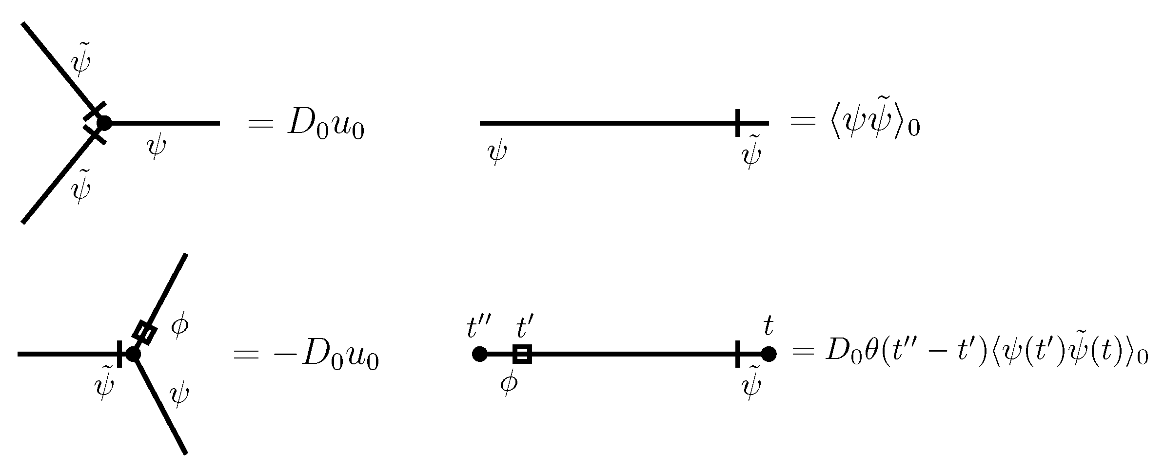
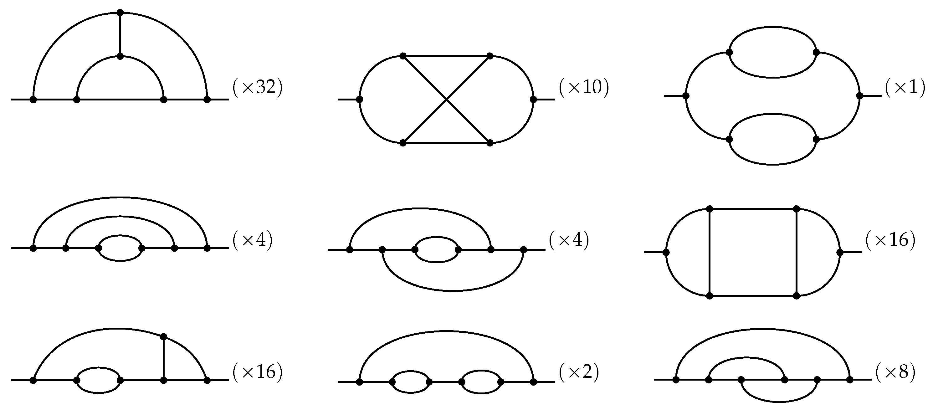
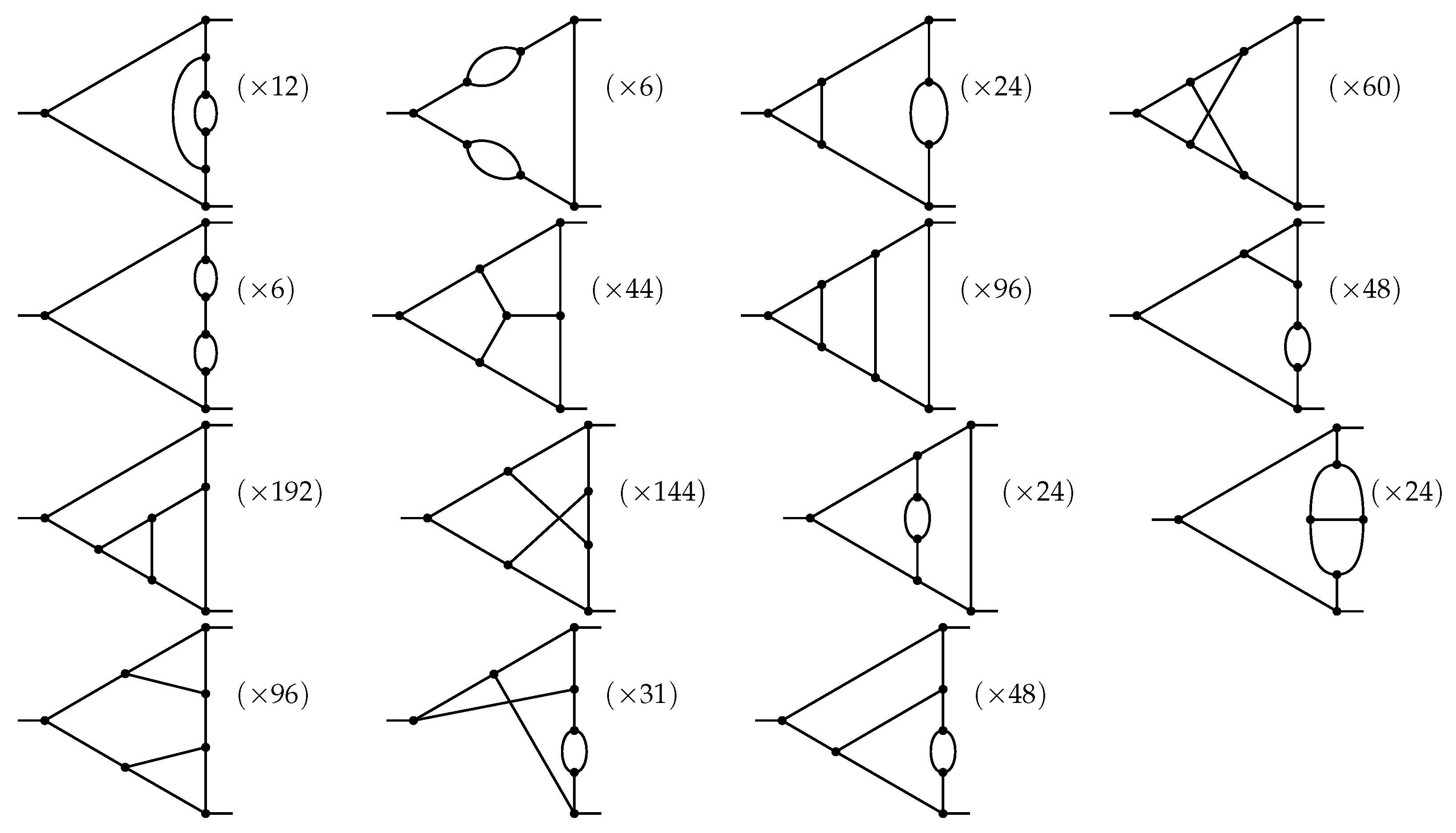
Table 1.
Canonical dimensions of the bare parameters and fields for the IP response functional (144).
Table 1.
Canonical dimensions of the bare parameters and fields for the IP response functional (144).
| Q | |||||||
|---|---|---|---|---|---|---|---|
| 1 | 0 | 2 | |||||
| 0 | 1 | 0 | 0 | 1 | 0 | 0 | |
| 1 | 2 | 0 | 2 |
Table 2.
Representation of two-loop Feynman graphs for self-energy employing a formalism based on Nickel indices. In the first column, the number in brackets corresponds to the Feynman diagram from Equations (157)–(162).
Table 2.
Representation of two-loop Feynman graphs for self-energy employing a formalism based on Nickel indices. In the first column, the number in brackets corresponds to the Feynman diagram from Equations (157)–(162).
| Diagram | Nickel Index | Symmetry Coefficient |
|---|---|---|
| (157) | 1 | |
| (158) | 1 | |
| (159) | 1 | |
| (160) | 1 | |
| (161) | 1 | |
| (162) | 1 |
Table 3.
The number of three-loop 1PI graphs for the IP model.
| IP | 1-Loop | 2-Loop | 3-Loop |
|---|---|---|---|
| 1 | 6 | 93 | |
| 1 | 36 | 957 |
Disclaimer/Publisher’s Note: The statements, opinions and data contained in all publications are solely those of the individual author(s) and contributor(s) and not of MDPI and/or the editor(s). MDPI and/or the editor(s) disclaim responsibility for any injury to people or property resulting from any ideas, methods, instructions or products referred to in the content. |
© 2023 by the authors. Licensee MDPI, Basel, Switzerland. This article is an open access article distributed under the terms and conditions of the Creative Commons Attribution (CC BY) license (https://creativecommons.org/licenses/by/4.0/).
Share and Cite
MDPI and ACS Style
Hnatič, M.; Honkonen, J.; Lučivjanský, T.; Mižišin, L. Universality Classes of Percolation Processes: Renormalization Group Approach. Symmetry 2023, 15, 1696. https://doi.org/10.3390/sym15091696
AMA Style
Hnatič M, Honkonen J, Lučivjanský T, Mižišin L. Universality Classes of Percolation Processes: Renormalization Group Approach. Symmetry. 2023; 15(9):1696. https://doi.org/10.3390/sym15091696
Chicago/Turabian StyleHnatič, Michal, Juha Honkonen, Tomáš Lučivjanský, and Lukáš Mižišin. 2023. "Universality Classes of Percolation Processes: Renormalization Group Approach" Symmetry 15, no. 9: 1696. https://doi.org/10.3390/sym15091696
Note that from the first issue of 2016, this journal uses article numbers instead of page numbers. See further details here.