
A Note on the Lambert W Function: Bernstein and Stieltjes Properties for a Creep Model in Linear Viscoelasticity


1
Department of Physics, University of Bologna, and INFN, Via Irnerio 46, I-40126 Bologna, Italy
2
Department of Mathematics, University of Bologna, Piazza Porta San Donato, I-40127 Bologna, Italy
3
Department de Mathematics, University of Oviedo, C Leopoldo Calvo Sotelo 18, 33007 Oviedo, Spain
*
Author to whom correspondence should be addressed.
Symmetry 2023, 15(9), 1654; https://doi.org/10.3390/sym15091654
Submission received: 10 July 2023
/
Revised: 17 August 2023
/
Accepted: 25 August 2023
/
Published: 26 August 2023
(This article belongs to the Special Issue Theory and Applications of Special Functions II)
Abstract
:The purpose of this note is to propose an application of the Lambert W function in linear viscoelasticity based on the Bernstein and Stieltjes properties of this function. In particular, we recognize the role of its main branch, , in a peculiar model of creep with two spectral functions in frequency that completely characterize the creep model. In order to calculate these spectral functions, it turns out that the conjugate symmetry property of the Lambert W function along its branch cut on the negative real axis is essential. We supplement our analysis by computing the corresponding relaxation function and providing the plots of all computed functions.
Keywords:
Lambert function; completely monotonic functions; Bernstein functions; Stieltjes functions; Laplace transform; Stieltjes transform; creep; linear viscoelasticityMSC:
33-00; 34M30; 42B10; 44A10; 44A101. Introduction
The Lambert function is defined as the root of the transcendental equation
The mathematical history of the W function goes back to the 18th century as outlined in the seminal paper [1] where the interested reader can be informed about the analytical and numerical properties of this function. Further details can be found in several papers, see, e.g., [2,3,4,5,6], Section 4.13 of the handbook [7], and in the recent book [8] with references therein. For our purposes, we outline the paper [9]. The applications are found in many areas of applied science as outlined, e.g., in [8,10,11] and references therein. Let us outline also the applications in probability, see, e.g., [12,13,14], which could be considered and possibly revised in view of the present results in linear viscoelasticity.
In our analysis, we restrict our attention to the main branch of the W function on the real semiaxis . We claim that the Lambert function can be a candidate involved as a possible model for dimensionless creep compliance (i.e., a material function) in linear viscoelasticity. Indeed, according to a previous idea of [15], the property of being a Bernstein function (that is, with a completely monotonic derivative) for such material function is proved to be fundamental as stated in Chap. 2 of the book [16] and references therein. In addition, the property of also being a Stieltjes function provides further results for this viscoelastic model that, as far as we know, are new in the framework of the literature of linear viscoelasticity.
The plan of this paper is as follows. In Section 2, we summarize the essentials of linear viscoelasticity in order to point out the properties of the rate of creep of our model based on the Lambert function. As a consequence, the rate of creep, being a completely monotonic (CM) function with the additional requirement to be a Stieltjes function, turns out to be expressed in terms of two different spectral functions. In Section 3, we carry out a numerical and analytical analysis of our new model based on the properties of the Lambert function. We also illustrate with plots the related quantities which can better characterize the model itself. The consistence of our results are validated with MATHEMATICA. In the Conclusions section, we summarize our final remarks.
2. Essentials of Linear Viscoelasticity
According to the theory of linear viscoelasticity, viscoelastic bodies are characterized by two different interrelated functions, called material functions, which are causal in time (i.e., null for ). The first material function is the creep compliance , defined as the strain response to a unit step function of stress. The second material function is the relaxation modulus , which is defined as the stress response to a unit step function of strain. For more details, see, e.g., [17,18,19] and the recent book [16].
Taking (thus ), a viscoelastic body is assumed to show a nonvanishing instantaneous response both in creep and relaxation tests. Therefore, it is convenient to introduce the following dimensionless functions and :
where is a non-negative increasing function with
and is a non-negative decreasing function with
The nondimensional quantity q takes into account a suitable scaling of the strain, according to convenience, in experimental rheology. However, in the following we assume for simplicity without loss of generality.
Viscoelastic bodies may be distinguished in solid like and fluid like, whether is finite or infinite, so that is nonzero or zero, respectively.
As pointed out in most treatises on linear viscoelasticity, (e.g., in [16,18,19]), the relaxation modulus can be derived from the corresponding creep compliance through the Volterra integral equation of the second kind
Therefore, according to (2), the nondimensional relaxation function obeys the Volterra integral equation
In the Appendix B, we calculate the solution of (6) by using the Laplace transform. Hereafter, we use the following notation for the Laplace transform pair:
where the sign ÷ denotes the juxtaposition of the function with its Laplace transform . In order to distinguish the Laplace transform, we use the same notation f for the original function, but overlined with a tilde and with the proper argument s.
It is quite usual to require the existence of positive retardation and relaxation spectra for the material functions and , as pointed out in the monograph [15]. This implies (as formerly proved in [20] and then revisited by [21], as well as in [16]) that and and consequently, the dimensionless functions and , turn out to be Bernstein and completely monotonic functions, respectively.
We recall that a completely monotonic (CM) function is a non-negative, infinitely derivable function whose derivatives alternate in sign for . Moreover, a Bernstein function is a non-negative function whose derivative is CM. According to Bernstein’s theorem, is the Laplace transform of a non-negative function, if and only if is a CM function (the interested reader is referred to the excellent monograph [22] for more details on the mathematical properties of CM functions). Apply Bernstein’s theorem to write the rate of creep as follows:
where and are both non-negative functions and denote the required spectra in frequency (r) and in time (), respectively.
Then, from (9), the time spectrum can be determined using the transformation , so that
We recognize that the Laplace transform of the rate of creep is the iterated Laplace transform of the frequency spectrum, that is, the Stieltjes transform of . Therefore, the Titchmarsh formula provides the inversion of the Stieltjes transform, see, e.g., [23]. Indeed, since is CM, taking into account (9) and (A10) with (3), we have for its Laplace transform:
and exchanging the order of integration, we finally obtain:
We thus recognize that is the inverse of the Stieltjes transform of . Under suitable conditions, the inversion can be obtained by the Titchmarsh formula. (This formula is found without names in [23]. However, in some papers and books, it is cited with several names, just Titchmarsh in [16], Stieltjes–Perron in [24], Gross–Levi in [25], Bobylev–Cercignani in [26]. In any case, it results as a simple exercise in complex analysis as stated in [27] for the Mittag-Leffler function.) Thus,
In addition, if is a Stieltjes function (i.e., the Laplace transform of a CM function), then turns out to be the Laplace transform of a non-negative function that we denote by . Indeed,
where we have applied
Therefore, from (13), and applying the Titchmarsh formula, we obtain
Hence, in the case that the rate of creep is a Stieltjes function, we have another spectral function related to the previous spectral function by a Laplace transformation.
3. Application of the Lambert Function in Linear Viscoelasticity
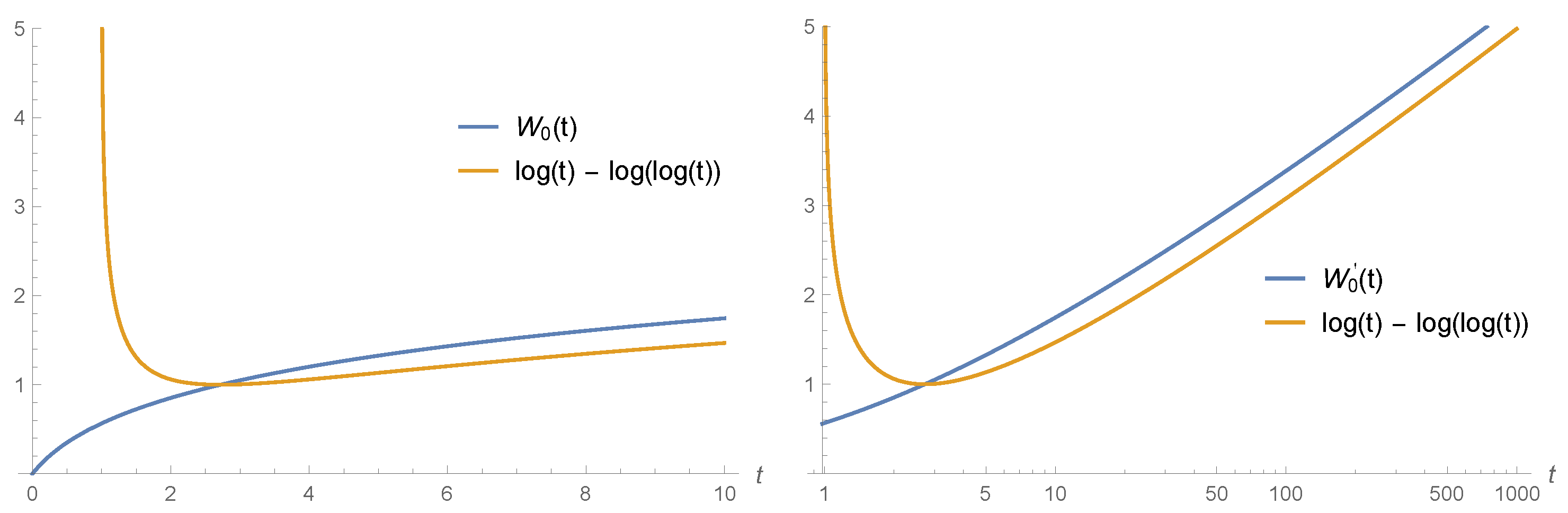
After recalling the properties of the Lambert W function, it is worth to see how its plot looks like compared with its asymptotic representation for large arguments. According to Figure 1, the function appears as a positive one, increasing from 0 at up to ∞ as . The two-term asymptotic representation,
fits the function slowly as .
We can see that the function is positive increasing up to ∞ according to its property of being a Bernstein function, that is, a non-negative function with a CM first derivative in , see, e.g., [4], p. 116. Furthermore, its derivative is known to be a Stieltjes function, that is, according to the definition stated in the previous section, a CM function represented by a real Laplace transform of a CM function, where both functions exhibit non-negative spectral functions, see [9].
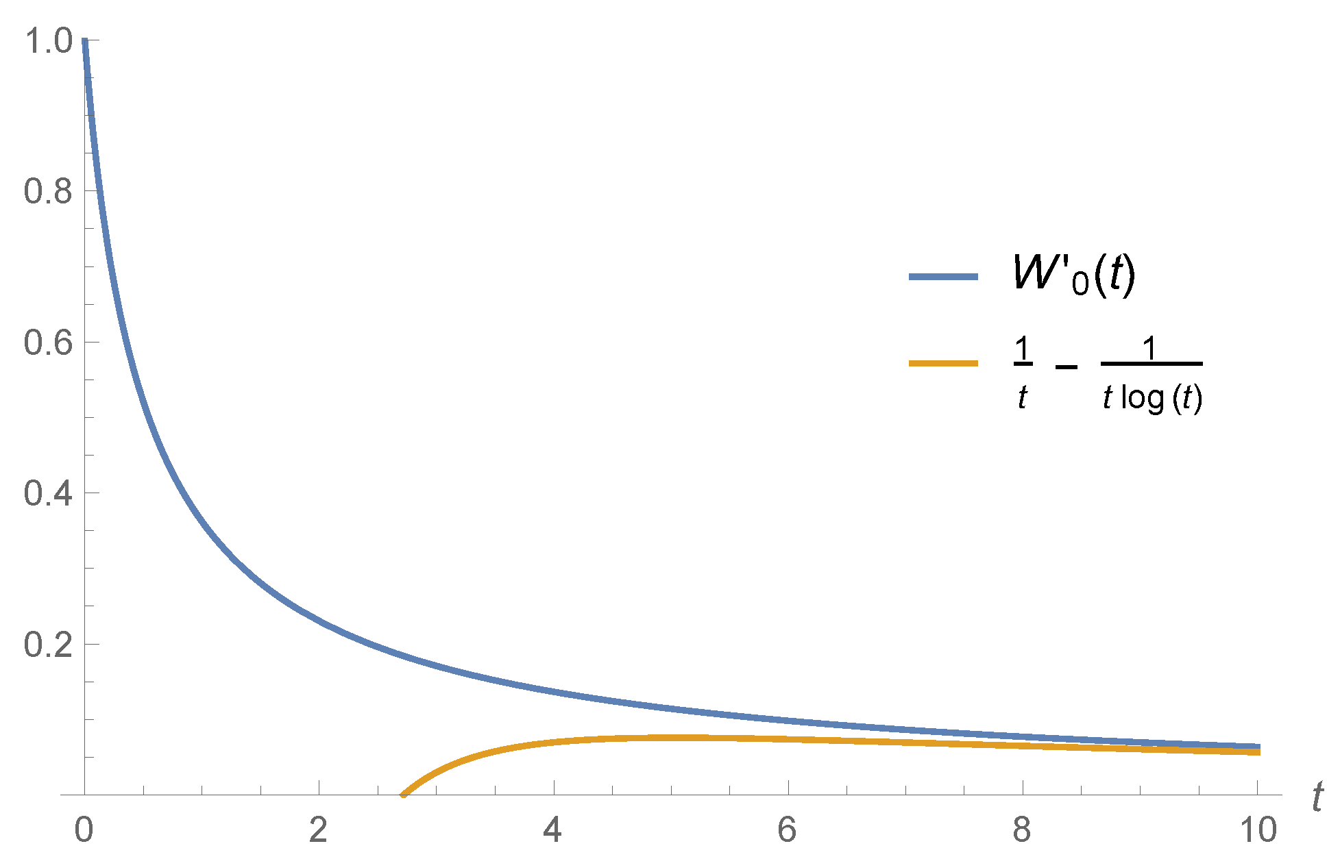
Differentiating in (1) and solving for , we obtain the following expressions for the derivative of :
and its two-term asymptotic representation is
The plots of the derivative of and its asymptotic representation are depicted in Figure 2.
In the proposed viscoelastic model, we assume for the creep that
From this assumption, and also taking into account that is a Stieltjes function, we derive the corresponding spectral functions and presented in the previous section. Indeed, the spectral function can be determined from (15) and (19), i.e.,
where is computed over or down the negative semiaxis that would be its branch cut in the complex plane.
According to the theory of the Titchmarsh formula, the function would be non-negative and continuous. However, our application of the Titchmarsh formula provides a non-negative function, but discontinuous, see Figure 3, where we note that for and non-negative for . In particular, is decreasing from ∞ in the limit to zero in the limit .
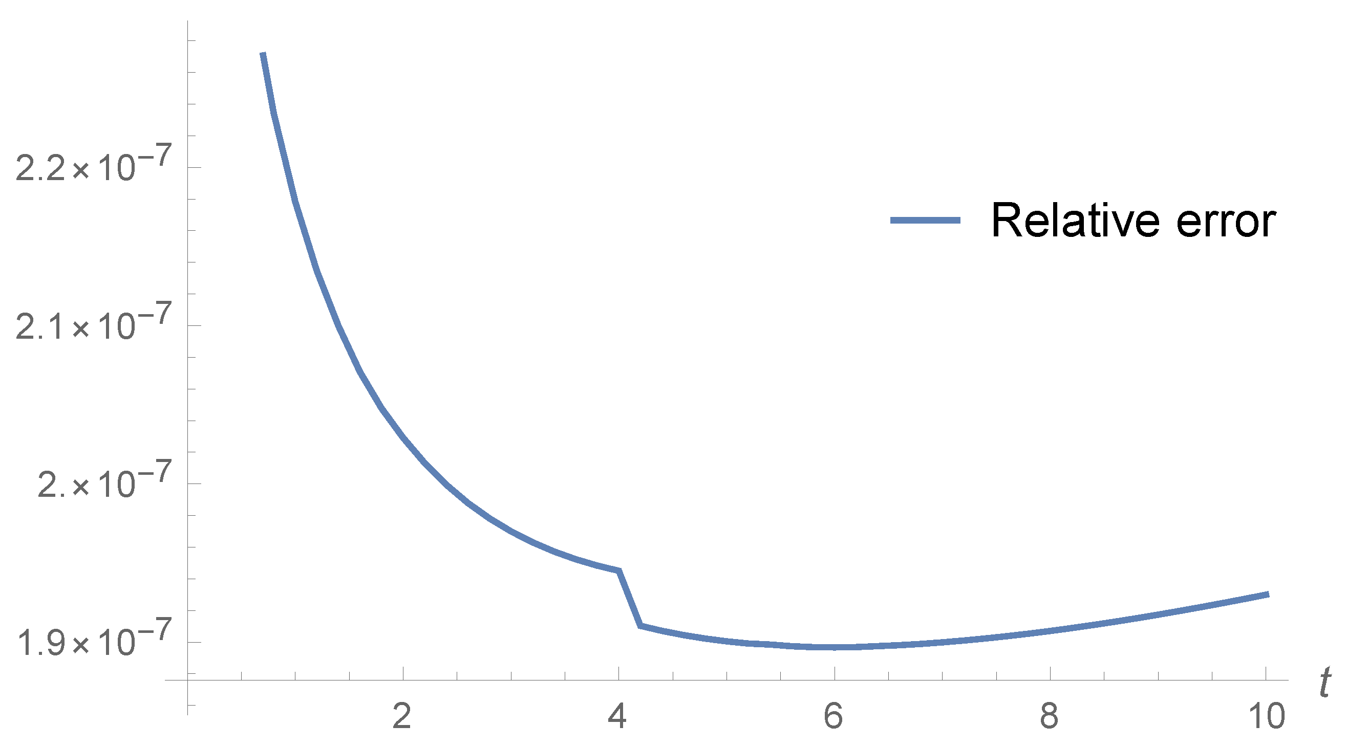
In order to validate the Stieltjes properties with the related Titchmarsh formula, we need to compute the iterated Laplace transform of the (discontinuous) spectral function and verify that it is the original derivative (see Equation (A15)) except for suitable small numerical errors. Indeed, by using MATHEMATICA, this result was verified because the relative error was small enough, as shown in Figure 4. Nonetheless, we obtained an alternative derivation of the function in Appendix A. It is worth noting that the conjugate symmetry property of the Lambert W function along its branch cut on the negative real axis, i.e., (A7), turns out to be essential for this derivation.
We note that a simple reasoning (validated by MATHEMATICA) provides the value of one for the Riemann generalized integral in the positive real semiaxis, that is
Indeed, taking into account (20), performing the change of variables , and knowing that , we have
Similar properties are shared by for , as validate by MATHEMATICA, but of course with different plots as it is shown in Figure 5.
Indeed, the value of the infinite integral of in the positive semiaxis is also one,
where this result is based on (13) for , (19), as well as the fact that , according to Figure 2.
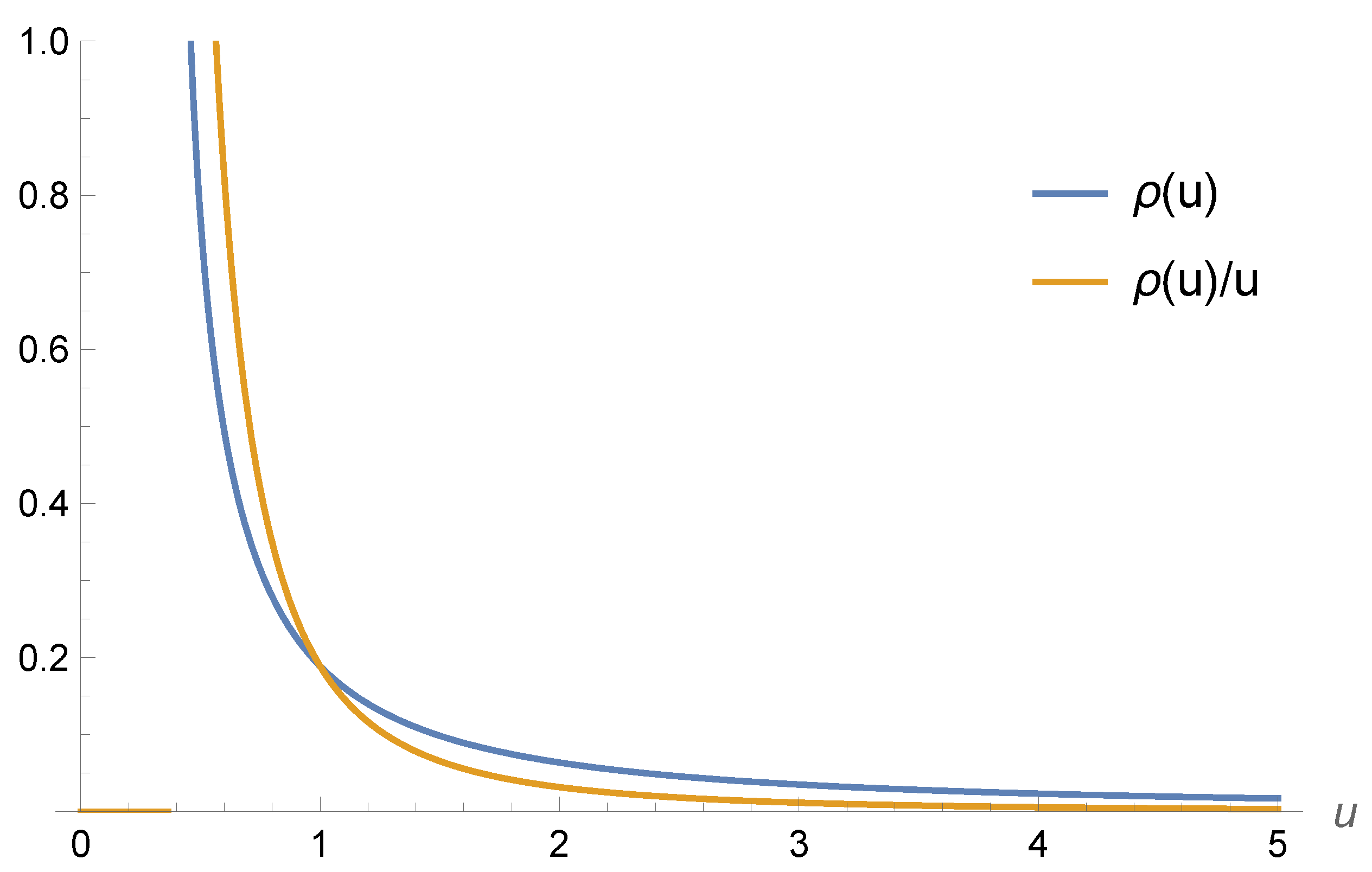
According to (12) and (19), we need the expression of the Laplace transform of in order to calculate the spectral function . However, the latter is not available in the literature. Nevertheless, we can numerically evaluate the spectral function from (14) with the expression given in (20) for the function, i.e.,
as it is shown in Figure 6. Nonetheless, since the function given in (20) is subjected to a numerical validation as discussed above, we provide an analytical derivation of (23) in Appendix A.
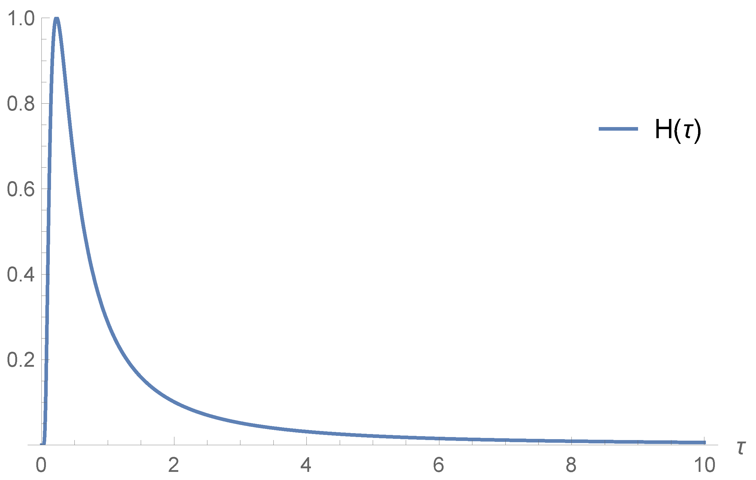
Figure 7 shows the plot of the spectral function in time.
We recognize that is not a CM function because its relation with in the transformation cannot preserve this relevant property.
4. Conclusions
In this paper, we pointed out some properties of the Lambert function taking advantage of the large existing literature on that function. In particular, we used these properties to propose a model in linear viscoelasticity that appears to be novel, as far as we know. This model was well characterized, as far as the creep was concerned, with two spectral functions. These spectral functions were numerically validated with MATHEMATICA, as well as analytically derived in Appendix A.
It is worth noting that this model provides an instructive slow-varying creep function, slower than a logarithmic law exhibited by the Lomintz and Becker models known in the geophysical literature, see [16], Section 2.9.1.
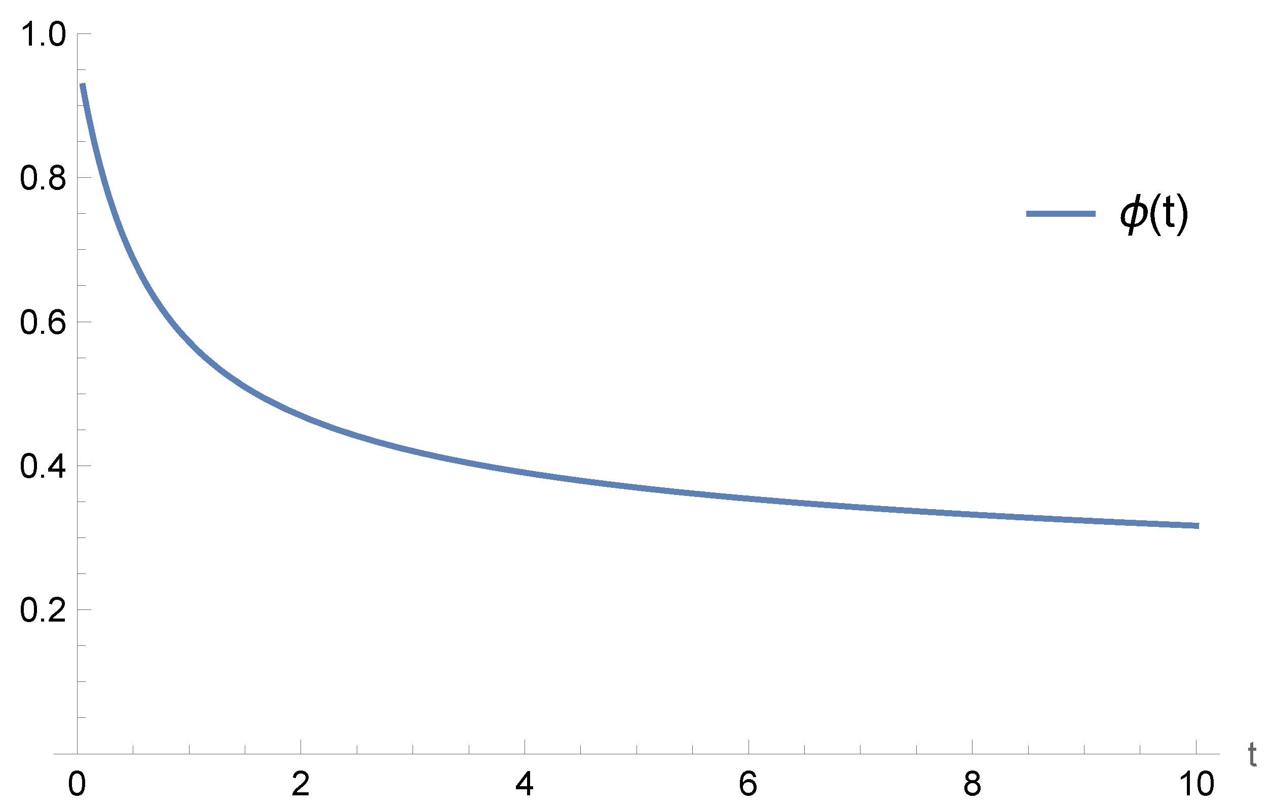
To complete the analysis of our model we provided the calculation of the corresponding relaxation function.
Author Contributions
Conceptualization, F.M.; methodology, F.M.; software, J.L.G.-S. and E.M.; validation, J.L.G.-S. and E.M.; formal analysis, J.L.G.-S.; investigation, F.M.; writing—original draft preparation, F.M.; writing—review and editing, J.L.G.-S.; supervision, F.M. All authors have read and agreed to the published version of the manuscript.
Funding
This research received no external funding.
Acknowledgments
The research activity of F. Mainardi has been carried out within the framework of the activities of the National Group of Mathematical Physics (GNFM, INdAM). The authors are grateful to R. Garra for useful discussions.
Conflicts of Interest
The authors declare no conflict of interest.
Abbreviations
The following abbreviations are used in this manuscript:
| CM | Completely monotonic |
Appendix A. Alternative Method for the Calculation of the Spectral Functions
Appendix A.1. Inverse Laplace Transform of
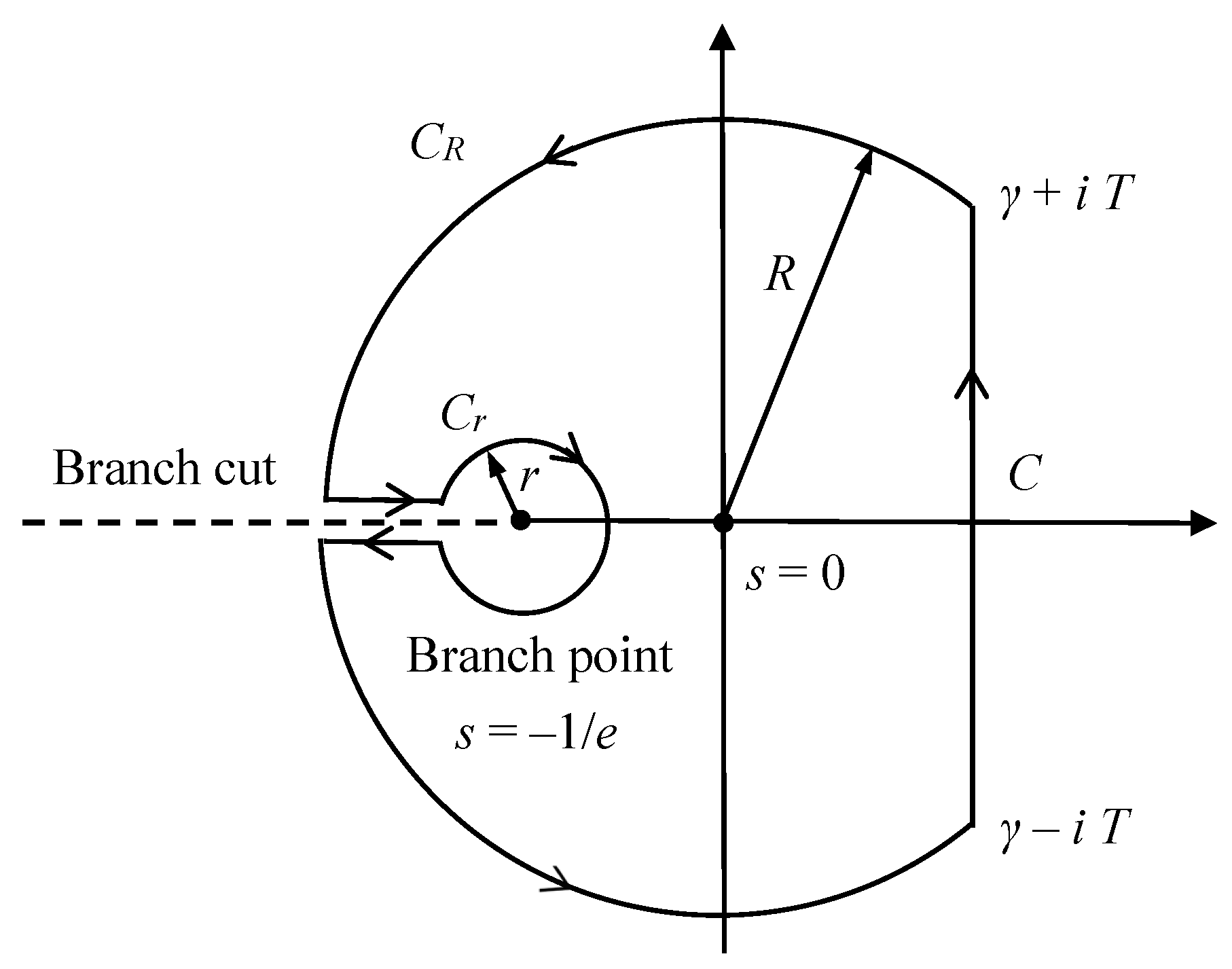
The inverse Laplace transform can be calculated by applying the Bromwich integral:
where the integration is calculated along the vertical line in the complex plane such that is greater than the real part of all singularities of . In our case, according to (17), we have
where has two singularities: and (since ). Note that is a simple pole and is a branch point. Consider the complex integral along the contour C depicted in Figure A1.
Figure A1.
Integration path.

Theorem A1
(Cauchy residue theorem). If is analytic within and on a simple, close contour C except at finitely many points lying in the interior of C, then
where the integral is taken in the positive direction.
Definition A1.
The function has a pole of order m at , if and only if
where is analytic at and .
Theorem A2
(Residues). If has a pole of order m at , then
Therefore, knowing that , we have
Now, consider the following Lemma [28] (Lemma 4.1).
Lemma A1.
If satisfies
and is a circular path of radius R centered at the origin, then, for , we have
On the other hand, applying the power series of about the point ,
and taking on , we have
thus
Performing the change of variables and taking into account that for , we obtain
We collect the results given in (A3), (A4), (A6) and (A8) and substitute them into (A2) to arrive at
Finally, we apply the following result [28] (Theorem 2.7).
Theorem A3.
Let f be continuous on and of exponential order α. If is piecewise continuous on , then
Therefore, in our case, since , we finally arrive at
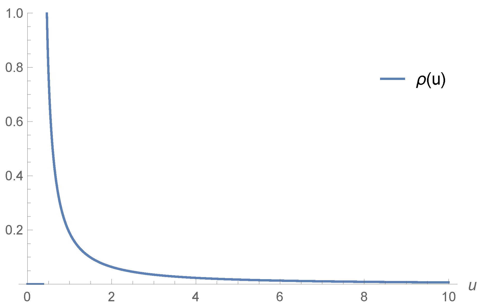
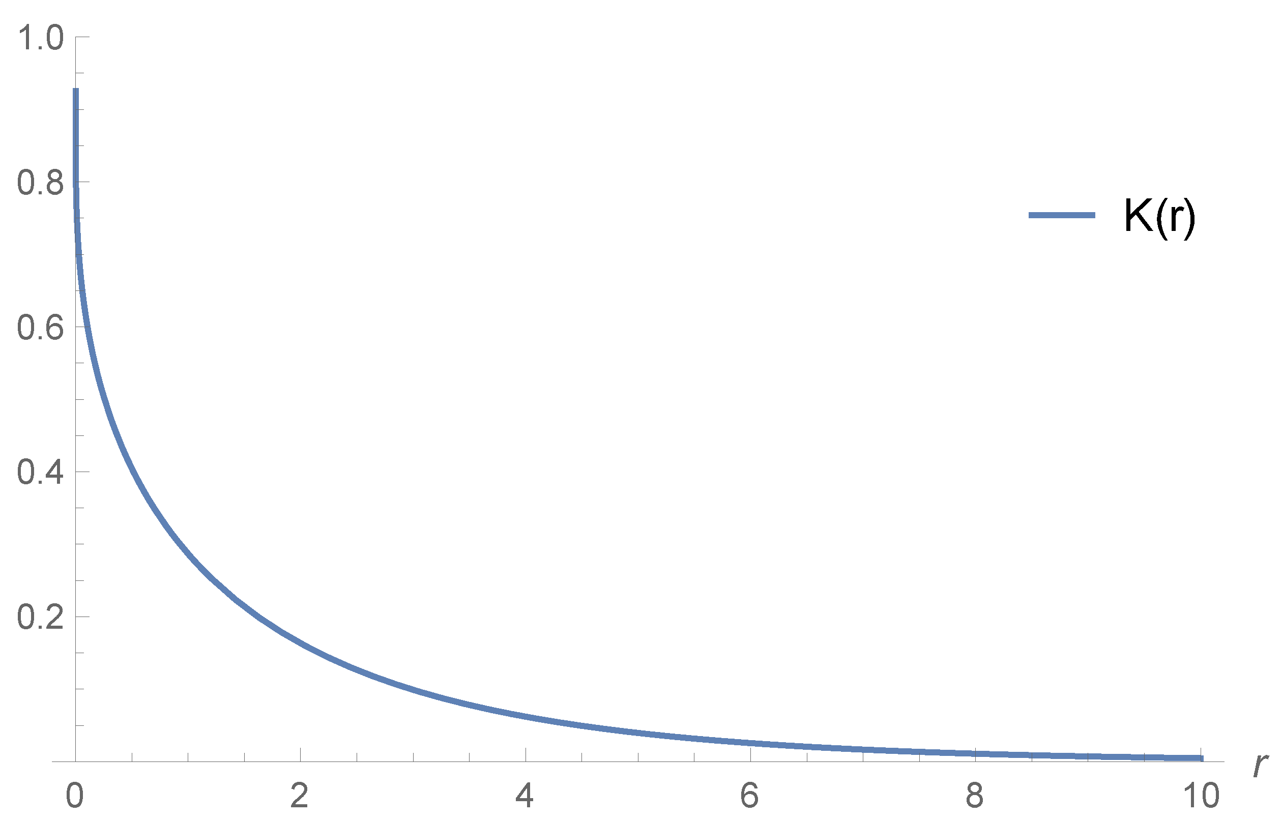
Appendix A.2. Calculation of K(r) and ρ(u)
On the one hand, we write (14) as
Appendix B. Calculation of
Let us solve (6), i.e.,
Theorem A4
(Convolution theorem). If f and g are piecewise continuous on and of exponential order α, then
where the convolution is given by the integral
Therefore, by applying the Laplace transform to (A18), we obtain
Solving for yields
References
- Corless, R.M.; Gonnet, G.H.; Hare, D.E.G.; Jeffrey, D.J.; Knuth, D.E. On the Lambert W function. Adv. Comput. Math. 1996, 51, 329–359. [Google Scholar] [CrossRef]
- Jeffrey, D.J.; Hare, D.E.G.; Corless, R.M. Unwinding the branches of the Lambert W function. Math. Sci. 1996, 21, 1–7. [Google Scholar]
- Kheyfits, A.I. Closed-form representations of the Lambert W function. Fract. Calc. Appl. Anal. 2004, 7, 177–190. [Google Scholar]
- Kalugin, G.A. Analytical Properties of W Lambert Function. Ph.D. Thesis, University of Western Ontario, London, ON, Canada, 2011. [Google Scholar]
- Kalugin, G.A.; Jeffrey, D.J. Unimodal sequences show that Lambert W is Bernstein. C. R. Math. Rep. Acad. Sci. Can. 2011, 33, 50–56. [Google Scholar]
- Kalugin, G.A.; Jeffrey, D.J. Series transformations to improve and extend convergence. In Proceedings of the 12th International Workshop CASC 2010, Tsakhkadzor, Armenia, 6–12 September 2010; pp. 131–147. [Google Scholar]
- Olver, F.W.J.; Lozier, D.W.; Boisvert, R.F.; Clark, C.W. NIST Handbook of Mathematical Functions; Cambridge University Press: Cambridge, UK, 2010. [Google Scholar]
- Mezö, I. The Lambert W Function, Its Generalizations and Applications; CRC Press: Boca Raton, FL, USA, 2022. [Google Scholar]
- Kalugin, G.A.; Jeffrey, D.J.; Corless, R.M.; Borwein, P.B. Stieltjes and other integral representations for functions of Lambert W. Integral Transform. Spec. Funct. 2012, 23, 581–593. [Google Scholar] [CrossRef]
- Valluri, S.R.; Jeffrey, D.J.; Corless, R.M. Some applications of the Lambert W function to physics. Can. J. Phys. 2000, 78, 823–831. [Google Scholar]
- Jordan, P.M. A note on the Lambert W-function: Applications in the mathematical and physical sciences. Contemp. Math. 2014, 618, 247–263. [Google Scholar]
- Pakes, A.G. Lambert’s W, infinite divisibility and Poisson mixtures. J. Math. Anal. Appl. 2011, 378, 480–492. [Google Scholar]
- Vinograadov, V. Some utilizations of Lambert W function in distribution theory. Commun. Stat.-Theory Methods 2013, 42, 2025–2043. [Google Scholar] [CrossRef]
- Pakes, A.G. The Lambert W function, Nuttall’s integral, and the Lambert law. Stat. Probab. Lett. 2018, 119, 53–60. [Google Scholar] [CrossRef]
- Gross, R. Mathematical Structure of the Theories of Viscoelasticity; Hermann: Paris, France, 1953. [Google Scholar]
- Mainardi, F. Fractional Calculus and Waves in Linear Viscoelastity, 2nd ed.; World Scientific: Singapore, 2022. [Google Scholar]
- Christensen, R.M. Theory of Viscoelasticity, 2nd ed.; Academic Press: New York, NY, USA, 1982. [Google Scholar]
- Pipkin, A.C. Lectures on Viscoelastic Theory, 2nd ed.; Springer: New York, NY, USA, 1986. [Google Scholar]
- Tschoegl, N.W. The Phenomenological Theory of Linear Viscoelastic Behavior; Springer: Heidelberg, Germany, 1989. [Google Scholar]
- Molinari, A. Viscoélasticité linéaire et fonctions complètement monotones. J. Méc. 1973, 12, 541–553. [Google Scholar]
- Hanyga, A. Viscous dissipation and completely monotonic relaxation moduli. Rheol. Acta 2005, 44, 614–621. [Google Scholar] [CrossRef]
- Schilling, R.L.; Song, R.; Vondracek, Z. Bernstein Functions. Theory and Applications, 2nd ed.; De Gruyter: Berlin, Germany, 2012. [Google Scholar]
- Widder, D.V. The Laplace Transform; Princeton University Press: Princeton, NJ, USA, 1946; pp. 325–391. [Google Scholar]
- Henrici, P. Applied and Computational Complex Analysis, Vol. 2; Wiley: New York, NY, USA, 1977; p. 591. [Google Scholar]
- Apelblat, A. Laplace Transforms and their Applications; Nova Science Publishing: New York, NY, USA, 2011. [Google Scholar]
- Aghili, A.; Masomi, M.R. Integral transforms method for solving F.S.I.es and P.F.D.es. Konuralp J. Math. 2014, 2, 45–62. [Google Scholar]
- Gorenflo, R.; Mainardi, F. Fractional calculus, integral and differential equations of fractional order. In Fractals and Fractional Calculus in Continuum Mechanics; Carpinteri, A., Mainardi, F., Eds.; Springer: Wien, Austria, 1997; pp. 223–276. [Google Scholar]
- Schiff, J.L. The Laplace Transform: Theory and Applications; Springer Science & Business Media: New York, NY, USA, 1999. [Google Scholar]
Figure 1.
The function versus dimensionless time compared with its two-term asymptotic representation. We have adopted linear scales in the left subfigure for , and in the right subfigure, log–log scales for .
Figure 1.
The function versus dimensionless time compared with its two-term asymptotic representation. We have adopted linear scales in the left subfigure for , and in the right subfigure, log–log scales for .

Figure 2.
The function versus dimensionless time compared with its two-term asymptotic representation for .
Figure 2.
The function versus dimensionless time compared with its two-term asymptotic representation for .

Figure 3.
The spectral function for .

Figure 4.
Relative error between the iterated Laplace transform of the spectral function and the function for .
Figure 4.
Relative error between the iterated Laplace transform of the spectral function and the function for .

Figure 5.
The spectral function compared with the function for .

Figure 6.
The plot of the spectral function for .

Figure 7.
The plot of the spectral function for .

Figure 8.
Dimensionless function for .

Disclaimer/Publisher’s Note: The statements, opinions and data contained in all publications are solely those of the individual author(s) and contributor(s) and not of MDPI and/or the editor(s). MDPI and/or the editor(s) disclaim responsibility for any injury to people or property resulting from any ideas, methods, instructions or products referred to in the content. |
© 2023 by the authors. Licensee MDPI, Basel, Switzerland. This article is an open access article distributed under the terms and conditions of the Creative Commons Attribution (CC BY) license (https://creativecommons.org/licenses/by/4.0/).
Share and Cite
MDPI and ACS Style
Mainardi, F.; Masina, E.; González-Santander, J.L. A Note on the Lambert W Function: Bernstein and Stieltjes Properties for a Creep Model in Linear Viscoelasticity. Symmetry 2023, 15, 1654. https://doi.org/10.3390/sym15091654
AMA Style
Mainardi F, Masina E, González-Santander JL. A Note on the Lambert W Function: Bernstein and Stieltjes Properties for a Creep Model in Linear Viscoelasticity. Symmetry. 2023; 15(9):1654. https://doi.org/10.3390/sym15091654
Chicago/Turabian StyleMainardi, Francesco, Enrico Masina, and Juan Luis González-Santander. 2023. "A Note on the Lambert W Function: Bernstein and Stieltjes Properties for a Creep Model in Linear Viscoelasticity" Symmetry 15, no. 9: 1654. https://doi.org/10.3390/sym15091654
Note that from the first issue of 2016, this journal uses article numbers instead of page numbers. See further details here.