
Automatic Brain Tumor Detection and Volume Estimation in Multimodal MRI Scans via a Symmetry Analysis

1
Department of Electrical and Electronics Engineering, Ankara University, 06830 Ankara, Turkey
2
Department of Biomedical Engineering, TOBB University of Economics and Technology, 06560 Ankara, Turkey
3
Department of Biomedical Engineering, Başkent University, 06790 Ankara, Turkey
*
Author to whom correspondence should be addressed.
Symmetry 2023, 15(8), 1586; https://doi.org/10.3390/sym15081586
Submission received: 30 April 2023
/
Revised: 16 June 2023
/
Accepted: 31 July 2023
/
Published: 14 August 2023
(This article belongs to the Section Life Sciences)
Abstract
:In this study, an automated medical decision support system is presented to assist physicians with accurate and immediate brain tumor detection, segmentation, and volume estimation from MRI which is very important in the success of surgical operations and treatment of brain tumor patients. In the proposed approach, first, tumor regions on MR images are labeled by an expert radiologist. Then, an automated medical decision support system is developed to extract brain tumor boundaries and to calculate their volumes by using multimodal MR images. One advantage of this study is that it provides an automated brain tumor detection and volume estimation algorithm that does not require user interactions by determining threshold values adaptively. Another advantage is that, because of the unsupervised approach, the proposed study realized tumor detection, segmentation, and volume estimation without using very large labeled training data. A brain tumor detection and segmentation algorithm is introduced that is based on the fact that the brain consists of two symmetrical hemispheres. Two main analyses, i.e., histogram and symmetry, were performed to automatically estimate tumor volume. The threshold values used for skull stripping were computed adaptively by examining the histogram distances between T1- and T1C-weighted brain MR images. Then, a symmetry analysis between the left and right brain lobes on FLAIR images was performed for whole tumor detection. The experiments were conducted on two brain MRI datasets, i.e., TCIA and BRATS. The experimental results were compared with the labeled expert results, which is known as the gold standard, to demonstrate the efficacy of the presented method. The performance evaluation results achieved accuracy values of 89.7% and 99.0%, and a Dice similarity coefficient value of 93.0% for whole tumor detection, active core detection, and volume estimation, respectively.
1. Introduction
Magnetic resonance imaging (MRI), which is one of the neuroimaging techniques used in clinics, has important roles in early diagnosis, treatment planning, and post-therapy assessment of abnormal brain tissues. MRI provides different image modalities via various acquisition protocols and parameters, so the same brain tissues can be visualized with different contrast and high resolution [1,2]. Due to the fact that healthy brain tissues and abnormal brain regions have similar intensity levels, it is difficult to determine brain tumor boundary in single-spectral MR images. Multi-spectral MRI scans which possess high resolution and contrast visualization can be useful for accurate detection of abnormal tumor boundary.
The first objective tool for radiologic assessment of treatment response in high-grade gliomas was originally published as the Macdonald criteria in 1990, which is based on the evaluation of tumor enhancement through CT. Besides, to standardize the assessment and reporting of results, objective evaluation of measurable and non-measurable disease relies on the use of 4 categories to describe response: complete response, partial response, stable disease, and progressive disease. These categories were introduced as the essential meas-urement of systemic cancer treatment response in the WHO criteria [3]. Through the years, the guidelines for brain tumor definition and assessment are defined and standardized by the Response Assessment in Neuro-Oncology (RANO) working group [3]. According to this new criteria, MR imaging added fundamental information about the non-enhancing component of the tumor, depicted on T2-weighted/FLAIR sequences, and became the standard neuroimaging technique used to assess treatment response in high-grade glio-mas [4]. However, RANO lacks sufficient detail for consistent implementation in certain aspects and leaves some issues from the original Macdonald guidelines unresolved. To provide the most accurate assessment of response to therapeutic intervention currently possible, it is essential that trial oncologists and radiologists not only have a solid under-standing of RANO guidelines, but also proper insight into the inherent limitations of the criteria [3].
Accurate segmentation of brain tumors is crucial for early diagnosis, treatment planning, and the recovery process of a patient by observing and tracking the size of the brain lesion [2,5,6]. In [7], manual and semi-automatic brain tumor volume estimation approaches were proposed. According to inter- and intra-operator agreement, evaluations showed that the semi-automated method provided faster and reliable results compared to the manual trace method. So, it was revealed that an automated brain tumor volume estimation for measuring serial tumor volumes in patients with high-grade brain neoplasms was faster and reliable compared to manual tracing. According to the World Health Organization and the Response Evaluation Criteria in Solid Tumors, tumor size measurement is used internationally as a surrogate marker for overall survival when following current response assessment protocols [8]. In the study by [8], volumetric, bidimensional, and unidimensional measurements for tumor size were realized by using contrast-enhanced T1-weighted MR images with recurrent malignant glioma receiving intravenous chemotherapy. The authors of the study in [9], presented a clinical evaluation of an automated segmentation approach for longitudinal brain tumor volumetry; they used automatic, machine learning-based segmentation method by subdividing a glioma into necrosis, edema, enhancing tumor, and non-enhancing tumor. The potential of an automatic segmentation method for brain tumor volumetry was confirmed via comparison against manual labeling by experts.
In addition to a multimodal analysis, automatic segmentation is also required for accurate detection of abnormal regions in brain MR images [6,10,11,12]. Manual tumor contouring realized by an expert is tedious work and requires attention, because examining MR sequences which have 50–200 slices for a patient takes a lot of time and the expert can be distracted during the long process. The fact that manual contouring depends on subjective judgements of various observers is also one of the disadvantages of manual segmentation [2].
Since multimodal MR images, which are obtained via different acquisition protocols, provide various information about abnormal tissue intensities, different types of MR sequence combinations have been used in tumor segmentation studies by many researchers. Refs [5,6,8,9,10,11,13,14,15,16] using multimodal MR images. Clark et al. [17] proposed a method segmenting tumor areas automatically via knowledge-based techniques using T1 weighted, T2 weighted and proton density (PD) images, Dou et al. [5] used fuzzy information fusion applied on T1 weighted, T2 weighted and PD images, Verma et al. [6] used support vector machine (SVM) method to segment the abnormal tissues of the brain from T1, T1C, T2, FLAIR and diffusion tensor imaging (DTI) modalities, Nie et al. [18] presented an approach based on spatial accuracy weighted hidden Markov random field and expectation maximization (SHE).
In other studies [2,11,12,19,20,21,22,23,24,25,26] researchers preferred to use single spectral images. Nabizadeh et al. [2] detected brain tumors from T1 and FLAIR images separately, Harati et al. [11] introduced the fuzzy connectedness algorithm to segment tumors from T1 post Gadolinium images, Dvorak et al. [12] and Prastawa et al. [20] used T2 weighted images, while Kaus et al. [19], Wang et al. [21] and Khotanlou et al. [22] used T1 weighted MR images, Khosravanian et al. [25] used fuzzy kernel level set method for 3D brain tumor seg-mentation from 40 FLAIR MR images, Nanda et al. [24] introduced a hybrid salien-cy-k-mean segmentation approach to segment brain tumors from FLAIR MRI.
There are some studies defining the importance of the symmetry/asymmetry in human brain hemispheres [27,28]. By using symmetry analysis in the brain Dvorak et al. [20] obtained brain tumors by using the SVM method, Khotanlou et al. [22] used spatial con-strained deformable models in addition to fuzzy classification, Ogretmenoglu et al. [14,15,16] introduced a brain tumor detection method using symmetry properties of two halves of the brain, Kermi et al. [23] proposed a method for brain tumor segmentation handling a hybrid method composed of fast bounding box, region growing and geodesic level-set methods, Khalil et al. [29] used a level set segmentation method based on dragonfly algorithm to segment brain tumors, Barzegar et al. [10] applied symmetry plane detection followed by similarity comparison.
Recently, in some studies in the literature, deep learning-based methods were used to detect brain tumors. Chen et al. [30] introduced a deep convolutional neural network which combines symmetry for brain tumor segmentation taking four modal MRI, Wu et al. [26] presented a study to segment brain tumors by using symmetric-driven adversarial network applied on T2 weighted MRI, Latif et al. [13] classify glioma type tumors by using deep learning, Athisayamani et al. [31] applied residual deep convolutional neural network (ResNet-152) to classify brain tumors, Pedada et al. [32] proposed a system to segment and classify brain tumor areas from multimodal MRI by using U-Net structure. Also, some analytical methods have been presented for symmetry analysis in literature [33,34,35] providing the solution of the application in different areas such as medical MRI.
There are many studies on brain tumor segmentation in the literature; however, there are still some gaps for methodological and clinical use. By eliminating these gaps, a robust decision support system on brain tumor diagnosis could be provided to the experts that they could be used in clinics. In the literature, brain tumor segmentation approaches using traditional segmentation methods generally cannot handle automated marking and selection of a tumor area from MR images, and they also generally require user assistance. Additionally, deep learning-based brain tumor detection methods necessitate large labeled MRI datasets for training. In addition, the studies on brain tumor detection, generally, have only focused on tumor segmentation or classification instead of tumor volume estimation. However, to assist the radiologist, volume estimation is a valuable skill of the decision support system on brain tumor diagnosis.
In this study, automated brain tumor detection and segmentation is proposed using a symmetry analysis from multimodal MRI. In addition, user interactions in the threshold assignment are eliminated by using a multimodal histogram analysis, so skull stripping is realized by an adaptive thresholding method. Tumor detection is realized via a symmetry analysis, and then segmentation and volume estimation processes are performed.
One of the contributions of this study is that it reveals the distinctiveness of the mean difference, area difference, and Bhattacharyya coefficient features extracted from MRI, thus proving that disruption in brain symmetry is one of the indicators of a brain tumor. Another contribution of this study is that the whole tumor including edema region and covering active core and necrotic core can be used as the mask to narrow the ROI (region of interest), thus reducing the search area as well as the algorithm execution time. Additionally, the unsupervised tumor segmentation method used in this study eliminates the need to use a large number of MRI data for the training phase required for supervised-based learning methods such as neural networks or deep learning. Finally, the proposed method can properly be used as a computer-aided system for assisting physicians with surgical planning and following the growing rate of brain tumor treatment duration.
The main novelty of this study is to provide a medical decision support system that performs all the operations sequentially for detecting MR slices containing tumors, determines tumor borders in these slices to calculate tumor area, and then estimates the volume of the tumor holding the contrast agent. Another novelty of this study is the use of symmetry-based features for brain tumor detection, segmentation, and volume estimation from MRI.
2. Materials and Methods
The algorithm was developed in the Matlab2021a environment and implemented on T1, T1C (T1 post gadolinium), and FLAIR modalities of brain MR images. The datasets used in this study are The Cancer Imaging Archive (TCIA) [36] and Brain Tumor Segmentation (BRATS) datasets. The TCIA dataset contains 529 brain MR images with 256 × 256 resolution and 0.938 mm pixel spacing that had been captured from 10 patients. Slices are differently weighted images per patient (approximately 53 scans per patient). Each patient has T1, T1C, and FLAIR MRI slices with 0.3 mm slice spacing and 0.3 mm slice thickness. The MRI slices in this dataset were labeled by an expert. In addition, the parts of the tumor that hold the contrast agent, called the active core regions, were drawn by a specialist on T1C MR images. The BRATS-2018 [37,38,39] dataset used in this study included 1705 MR images (155 scans per patient) consisting of skull-stripped images with T1, T1C, and FLAIR modalities.
This study’s proposal depends on an unsupervised slice-level segmentation algorithm; thus, the MRI datasets consisted of 529 and 1705 MRI slices per each MRI sequence. The experimental results, considering the high accuracy of the slice-level algorithm performed on 2234 MRI slices, showed that the size of the dataset was satisfactory enough to make conclusions about tumor detection, segmentation, and volume estimation.
The proposed brain tumor detection and volume estimation algorithm consists of six main stages: median filtering, skull stripping, symmetry analysis, whole tumor segmentation, active core segmentation, and volume estimation. The proposed brain tumor detection and volume estimation algorithm flowchart is given in Figure 1. Initially, noise reduction of the T1, T1C, and FLAIR MR images was realized by median filtering, since an amount of impulsive noises naturally affects MR image slices. The original T1, T1C, and FLAIR MR slices and median filtering results are shown in Figure 2 as an example. Secondly, skull parts of the multimodal brain MR slices were extracted by an adaptive thresholding method. The threshold values were obtained by using histograms of the T1 and T1C images. Third, a symmetry analysis applied on the FLAIR images was performed to detect and label tumor-containing MR slices according to asymmetry scores. Fourth, whole tumor segmentation was realized by using fuzzy c-means (FCM) clustering on the FLAIR MR slices labeled as tumor containing. Fifth, the obtained whole tumor regions were used as the ROI mask for active core detection and segmentation. Active core segmentation relies on the FCM clustering method applied on T1C MRI. Finally, after calculating the areas of the tumor in each MR slice for each patient individually, a volume estimation of the tumor active core was performed by using the calculated areas and also the spacing between slices, and the slice thickness parameters were obtained from the Digital Imaging and Communications in Medicine (DICOM) file.
2.1. Histogram Analysis for Skull Stripping
MR images in the TCIA dataset contained brain skull regions, while the BRATS dataset consisted of skull-stripped MR images. So, to remove these parts, a histogram analysis was performed using the T1 and T1C images. The aim of a histogram analysis is to obtain the threshold values automatically by calculating differences between the histogram values of the T1- and T1C-weighted MR images. The framework of the histogram analysis is given in Figure 3. Initially, histogram matching was performed on the T1 and T1C images, and then differences in the histograms were calculated. The maximum intensity level in the difference graph was assigned as the threshold value for a skull removal operation. Figure 3 also shows the determined threshold value on the histogram difference graph for a sample brain slice.
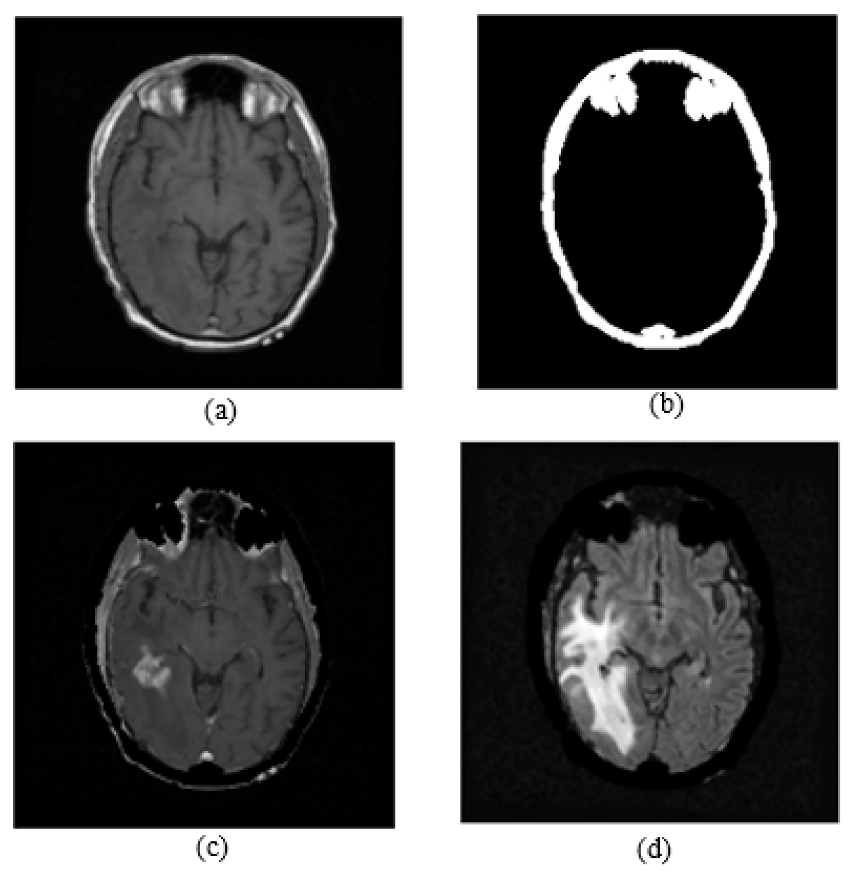
Non-brain regions such as the skull, orbital fat, and sclera in the brain MR images led to confusion in the tumor detection process, because these irrelevant parts have the same intensity level as tumor regions. In the T1C images, the skull, eyes, and tumor regions have high intensity level, while in the T1 images, only the skull and eye regions have high intensity, so the T1 images were used as a skull-stripping mask to remove irrelevant regions. A skull stripping block diagram is shown in Figure 4. To obtain the skull-stripping mask, an adaptive thresholding operation was applied to the T1-weighted images by using the threshold values assigned automatically in the histogram analysis part of the algorithm. A T1 image and the obtained skull stripping mask are shown in Figure 4. After obtaining the skull-stripping mask, the skull and eye regions of the FLAIR images were removed by a masking operation. Figure 5 shows a T1 image, a skull stripping mask, a skull-stripped T1C image, and a skull-stripped FLAIR image are given.
2.2. Symmetry Analysis for Tumor Detection
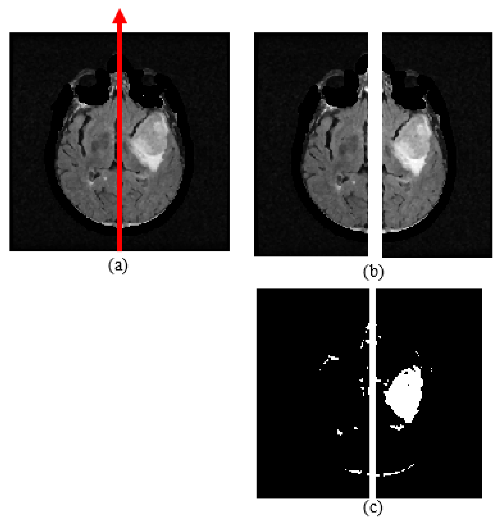
The aim of conducting the symmetry analysis is to obtain symmetry properties between the left and right brain halves. By using this analysis, a possible dissimilarity coming from a defect in a brain part, such as a tumor, can be observed between halves. Brain tumors cause edema that surrounds the abnormal region. The edema region is a high intensity level in the FLAIR modality, so the defected area in this region can be clearly observed in FLAIR images. In this study, the symmetry of two halves was examined using skull-stripped FLAIR images. A brain hemisphere including a tumor causes symmetry anomaly between the left and right parts of the FLAIR images. It is assumed that the mid-sagittal plane is a vertical line that divides the MR slice into two equal parts, so this vertical line is assigned as the geometrical symmetry axis, as shown in Figure 6a. The hemisphere containing a whole tumor is found by comparing the symmetry-based features, which are mean, area, and the Bhattacharyya coefficient (BC). While the Bhattacharyya coefficient and mean represent gray level characteristics, the area is used for examining binary characteristics of the MR image.
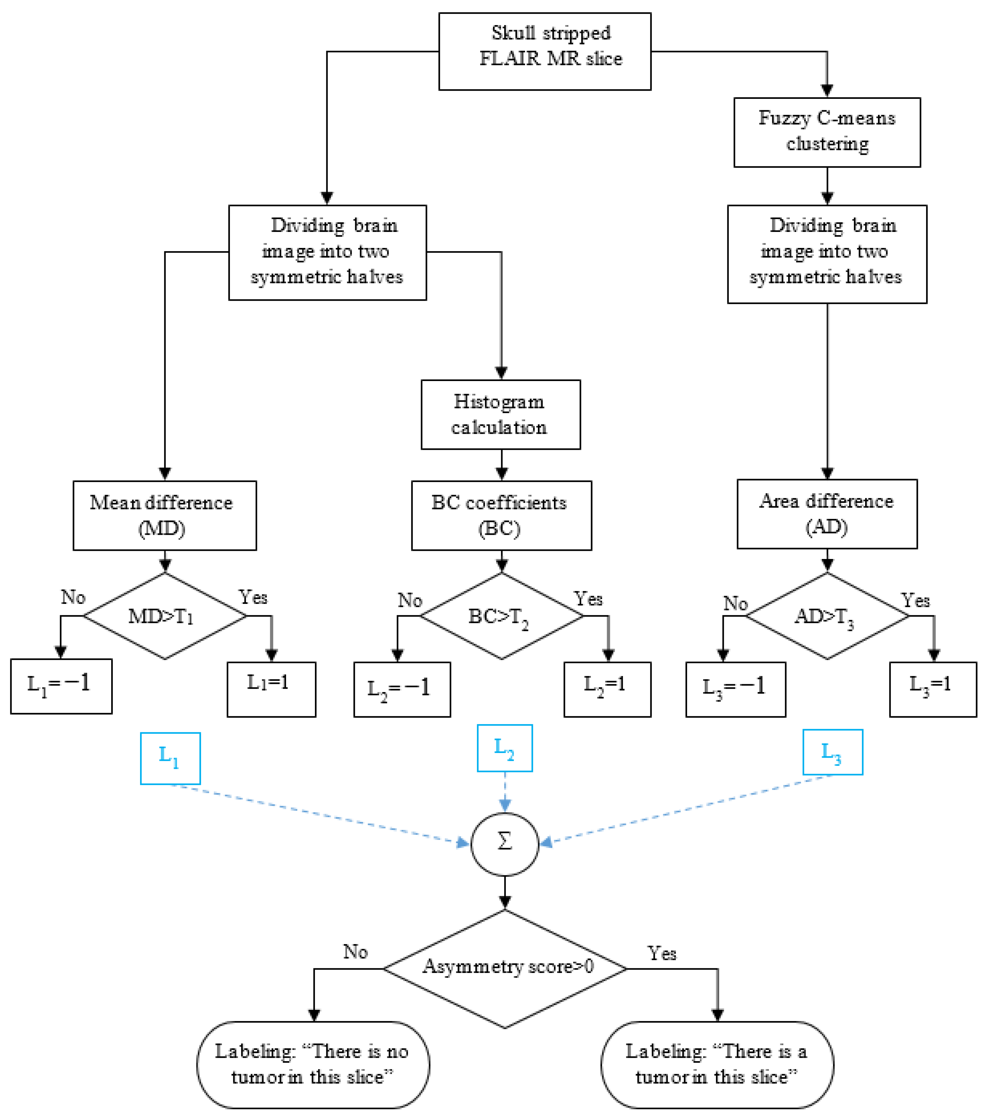
The symmetry analysis stage of the algorithm is processed according to the framework given in Figure 7. Initially, the FCM clustering method is applied on the skull-stripped FLAIR MR images, then the binary image is divided into two equal parts. The area difference (AD) is calculated from this binary left and right hemisphere images. In addition, the gray level, skull-stripped FLAIR MR image is divided into two equal halves, then the mean difference (MD) of the left and right part is calculated. In addition, histograms of the gray level parts are calculated, and then BC is calculated. After obtaining MD, BC, and AD values, L1, L2, and L3 labels are assigned as 1 or −1 according to threshold levels T1, T2, and T3, respectively. Then, the asymmetry score is obtained by summing these labels. Whole tumor detection in each FLAIR slice of a patient is realized according to the asymmetry score.
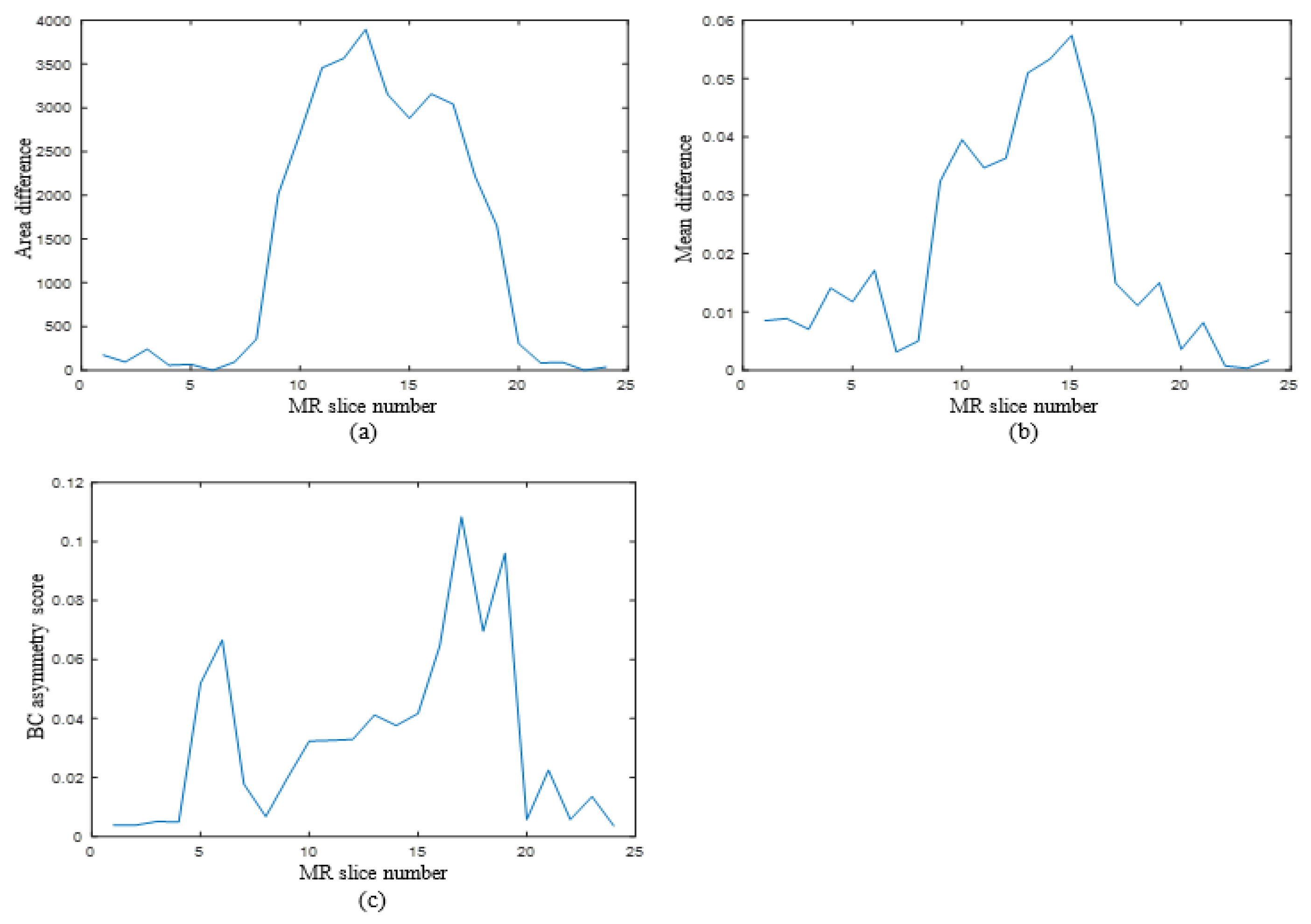
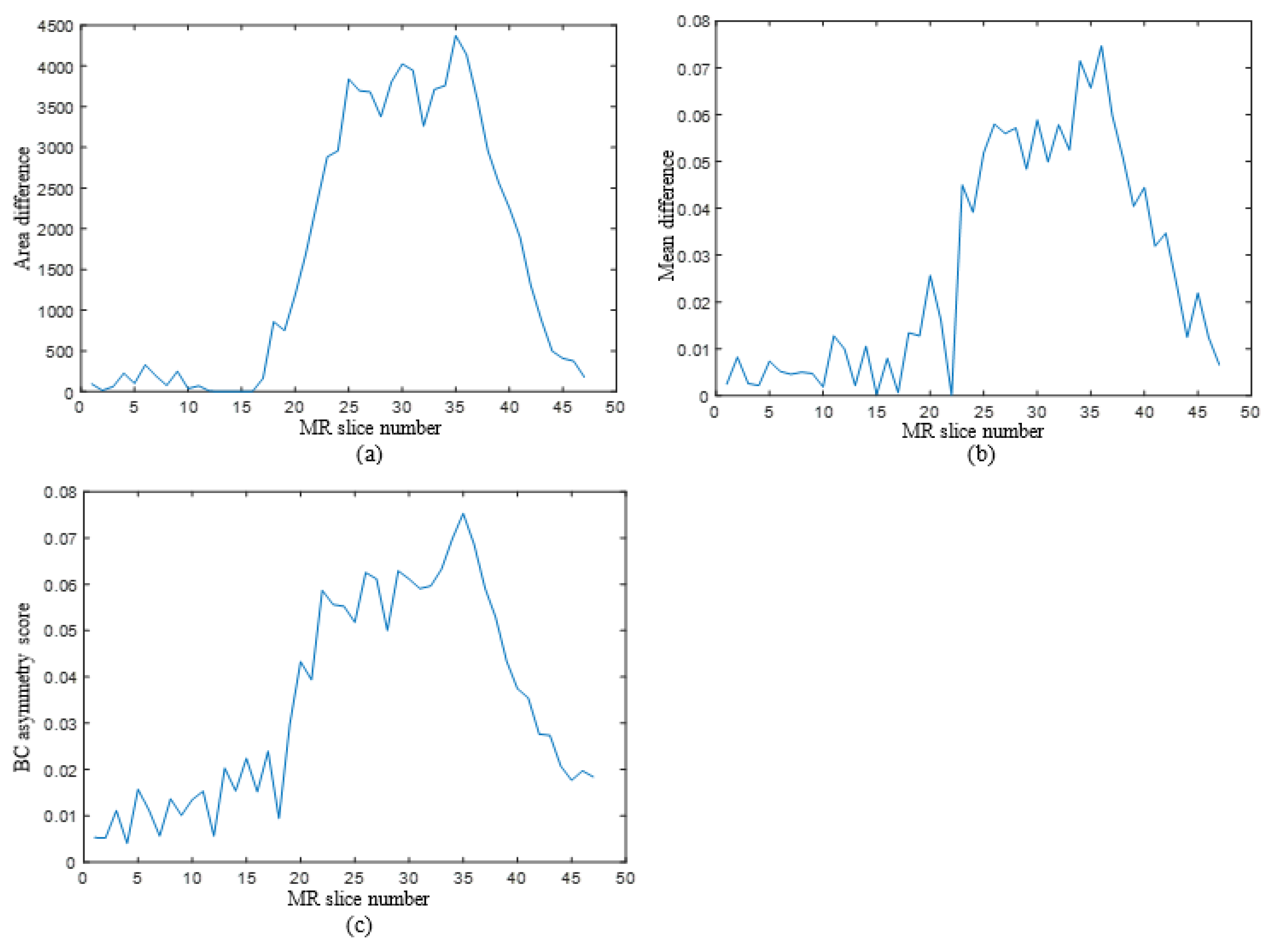
Area difference, mean difference, and BC asymmetry score graphs for two different patients are given in Figure 8 and Figure 9. As can be seen in these figures, graphs of all three features, i.e., MD, BC, and AD, have similar trends for both patients, since MD, BC and AD values are higher in MR sections containing tumors. The experimental results show that MD, BC, and AD values increased between FLAIR slices including tumor. So, it was decided to use these three distinguishing features in the symmetry analysis algorithm to detect brain tumor.
To find the area difference, the FCM clustering method is applied on the skull-stripped FLAIR image, then the binary MR slice obtained is separated into two equal halves via the vertical symmetry axis (Figure 6). Then, the left side area is subtracted from the right side area. FCM is an unsupervised clustering method, which is frequently used in medical image segmentation. Similar pixels are grouped into clusters in terms of their fuzzy memberships via fuzzy c-means clustering technique [40]. FCM is an iterative algorithm for the purpose of minimizing a cost function that is given in Equation (12). The cost function depends on the distance of the pixels to the cluster centers. In Equation (1), N, c, and represent the number of pixels, the number of clusters, and the jth pixel intensity, respectively. In this study, cluster number, c, is assigned as 3, represents the membership of the which is in the ith cluster, represents the ith cluster center, and m controls the fuzziness and it takes a constant value. Membership function and cluster centers are recalculated at every iteration by the formulas given in Equations (2) and (3) [40]:
The mean difference and the BC values are obtained from gray level skull-stripped FLAIR images by using (4) and (5), respectively. The operation of dividing an image into left and right halves is also applied on the gray level FLAIR image (Figure 6). Means of both halves are calculated, then the mean differences of the two halves are obtained via a subtraction operation. BC values are obtained using the histograms of the left and right parts of the MR slice. M, which is given in Equation (11), represents the total number of pixels, while x represents pixel intensity. I, which is given in Equation (12), represents the highest intensity value, while p(i) and q(i) represent normalized histogram values.
2.3. Whole Tumor Segmentation
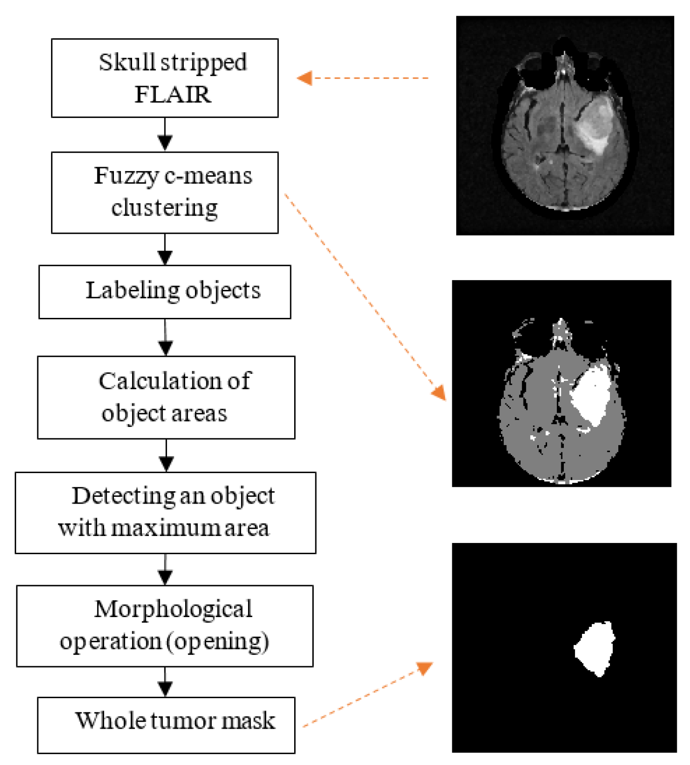
Edema associated with brain tumors includes the tumor and its boundaries, so to restrict the area of the tumor segmentation process, the whole tumor mask is obtained from FLAIR images at this stage. A flowchart of the whole tumor segmentation process is presented in Figure 10. Initially, fuzzy c-means clustering is applied on a skull-stripped FLAIR image, so three main clusters are obtained, i.e., the whole tumor region, the brain region excluding the whole tumor, and the background region. Secondly, each cluster is labeled via connected-component labeling in terms of pixel 8-connectivity, then the areas of each of the labeled regions are calculated. Since the whole tumor region has the smallest area, the region with smallest area is assigned as the whole tumor mask. Finally, the morphological opening operation is applied on the edema mask to remove residuals.
2.4. Active Core Segmentation and Volume Estimation
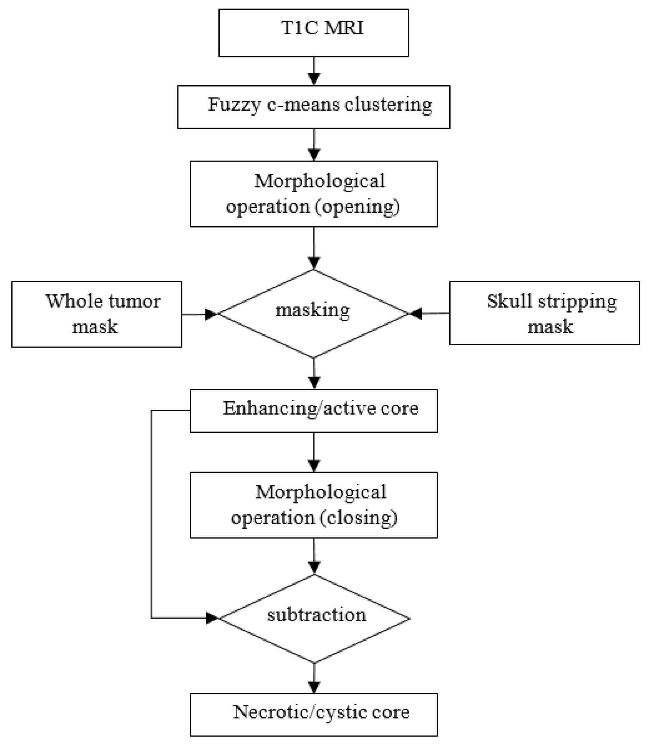
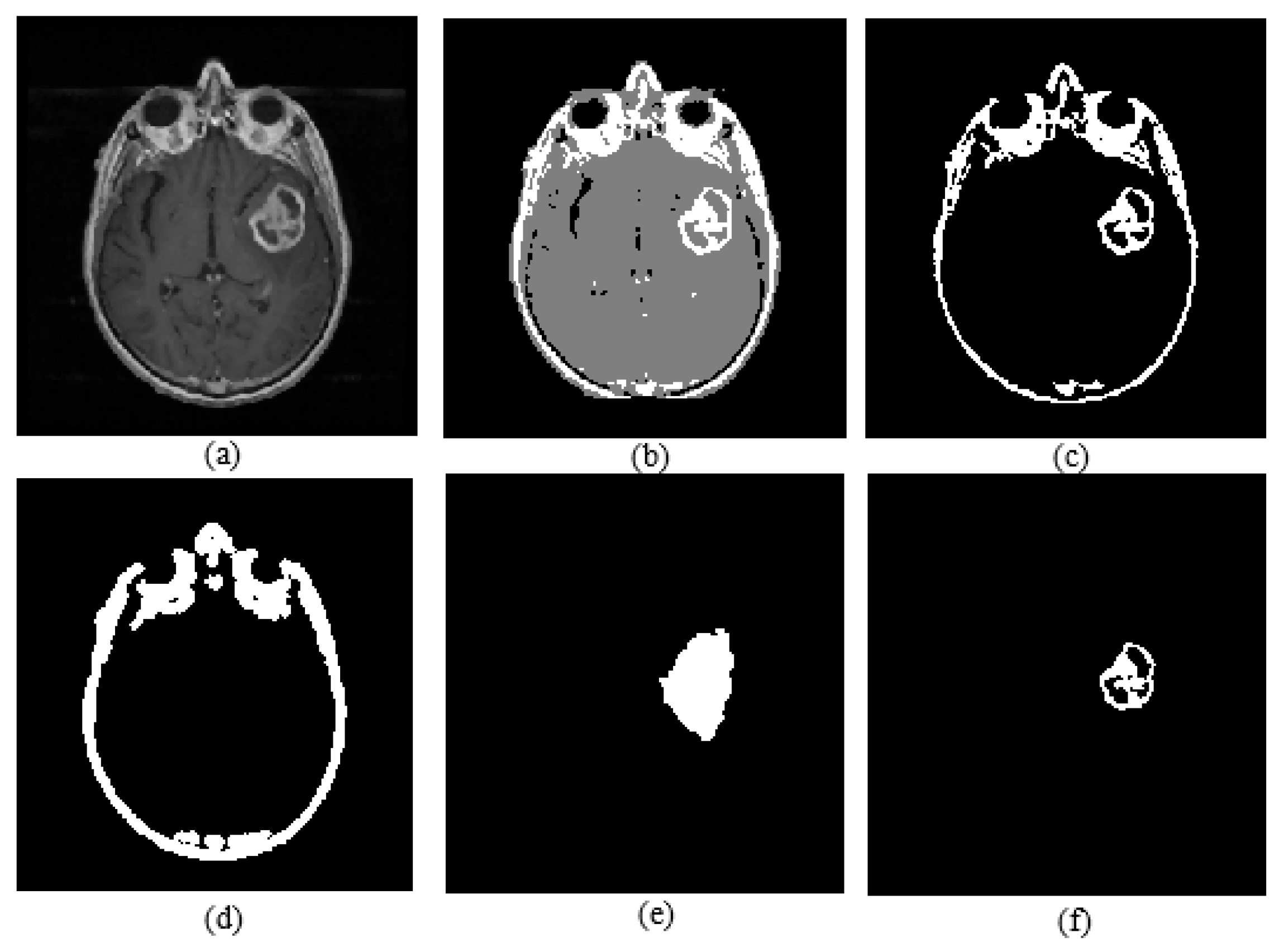
Active core segmentation and the volume estimation stage involve masking and FCM clustering operations, as outlined in Figure 11. The T1C image is converted to a binary image via FCM and a morphological opening operation (Figure 12c), and then skull stripping and whole tumor masks (Figure 12d,e) are applied on this image to obtain the enhancing/active core (Figure 12f). To obtain the necrotic/cystic core, a morphological closing operation is applied on the active core region (Figure 13c), then the active core is subtracted from this image (Figure 13d).
After extracting tumor regions, areas of these regions are calculated using the formula given in Equation (6). It is assumed that all the segmented tumor regions of a patient are superimposed, so these layers compose the volumetric structure of the tumor. Volume estimation is realized using the calculated real tumor areas and information, which are slice thickness, spacing between slices, and pixel spacing obtained from the DICOM header. In this work, 0.938 mm pixel spacing, 3 mm slice thickness, and 3 mm spacing between slices were used according to the DICOM file of the MR images of TCIA dataset. Real tumor area (A) is calculated via Equation (6) and volume estimation formula is given in Equation (7) in which N represents the number of slices:
3. Results
The proposed algorithm was implemented on MATLAB 2021a, and the process took 258.75 s per patient (258.75/53 = 4.88 s per slice). The computer used for implementation was an Intel Core i7, 2.60 GHz processor with 16.0 GB RAM. The proposed algorithm was applied on TCIA and BRATS-2018 datasets; 529 T1, 529 T1C, and 529 FLAIR modality axial brain MR images of 10 patients, and 1705 T1, 1705 T1C, and 1705 FLAIR modality axial brain MR images of 11 patients were used from the TCIA [36] and BRATS-2018 [37,38,39] datasets, respectively. An expert radiologist labeled all test MRI data manually, over approximately a month. The datasets consisted of slices with no tumor and included tumors that were in different locations, with different shapes and sizes. The algorithm developed was implemented on MATLAB 2021a. Boundary drawings of the active core area and labeling of each MR slice by detecting slices containing tumor were prepared by an expert, which is regarded to be a gold standard for evaluation of the proposed system. The performance analysis investigated sensitivity, specificity, the Jaccard coefficient (overlap fraction), and the Dice similarity coefficient. Performance metric formulas are given in Equations (8)–(12), and the TP, TN, FP, and FN terms used in these equations represent true positive, true negative, false positive, and false negative, respectively:
The detection of slices containing active core tumor and the volume estimation results, which were compared with the manual segmentations of an expert, are displayed via performance metrics. Performance metrics quantify the degree of congruence between the manual labeling and segmentation of an expert and the labeling and segmentation by the proposed system. Slices with the tumor identification algorithm evaluation depend on a slice-level analysis, while the volume estimation evaluation is based on a pixel-level analysis. The results and performance analysis of the detection of slices containing tumor algorithm are displayed in Table 1 and Table 2, respectively. For the tumor detection algorithm, the threshold values of the MD, BC, and AD features, represented by T1, T2, and T3, were assigned as 0.02, 0.02, and 600. These threshold values were determined experimentally. In Table 1, the total number of slices and the number of slices containing tumor per patient labeled by the expert are shown.
In addition, in Table 1, true positive (TP) represents the number of slices labeled as tumor by the expert and the proposed system; false negative (FN) represents the number of slices that the expert labels as containing tumor while the proposed system labels as no tumor; false positive (FP) represents the number of slices that the proposed system labels as containing tumor while the expert labels as no tumor; and true negative (TN) represents the number of slices labeled as no tumor by the expert and the proposed system.
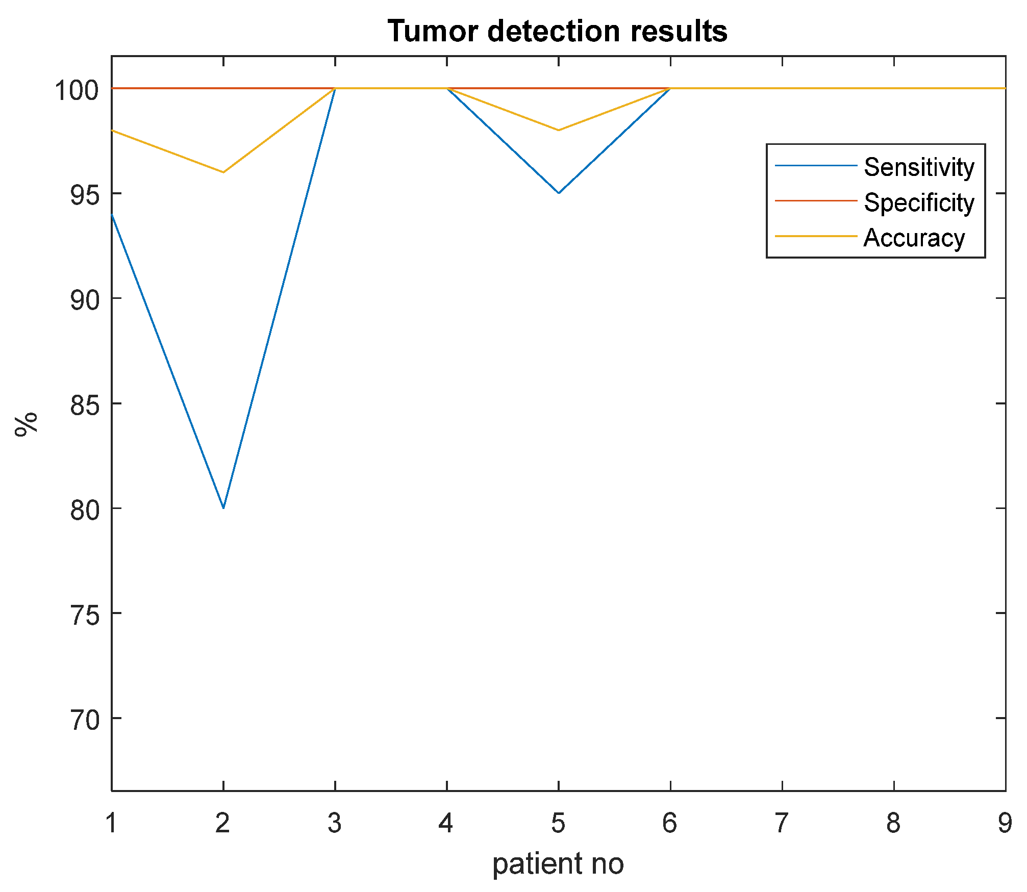
In Table 2, sensitivity is the probability that the proposed method identifies the slices with tumor in which the tumor is present. Specificity is the probability that the proposed method designates the slices without tumor in which the tumor is absent in reality. Accuracy is the ratio of the number of correct identifications to the total number of slices. The sensitivity, specificity, and accuracy of the detection of slices containing tumor algorithm are 97%, 100%, and 99%, respectively. For explaining clearly, the values in Table 2 were re-plotted in Figure 14. It can be seen from this figure that the smallest accuracy and sensitivity are obtained for Patient 2. The reason for this low accuracy result is that the related MR images do not have enough resolution by comparing the other examples in the dataset. Moreover, this active core tumor region cannot be discriminated easily from the background in these images because of insufficient contrast agent hold at that area.
The area estimation results for each MR slice of two patients from our dataset are reported in Table 3 and Table 4 as examples. As can be seen from Table 3 and Table 4, the cross-section area of the tumor increases towards the MR image showing the mid-section of the brain, while it decreases towards the lower sections, with the same logic. The tumor cross-section area in the 31st MR section of the patient in Example 1 (Table 3) is larger than that in the 37th section.
In these tables (Table 3 and Table 4), TP values represent the number of pixels in which both the expert and the proposed system label the same pixels as a tumor. FN values represent the number of pixels in which the expert labels the pixels as a tumor while the proposed system labels them as a background pixel. FP values represent the number of pixels in which the proposed system labels the pixels as a tumor while the expert labels them as a background pixel; and TN values represent the number of pixels in which both the expert and the proposed system label the pixels as a background. Sensitivity indicates the probability that the proposed system detects the tumor pixels that are also detected by the expert. Jaccard coefficient is the ratio of the intersection set of tumor pixels labeled by both the expert and the proposed system to their union set. The Dice similarity coefficient measures the portion of the correctly detected tumor pixels in the overall detected tumor pixels.
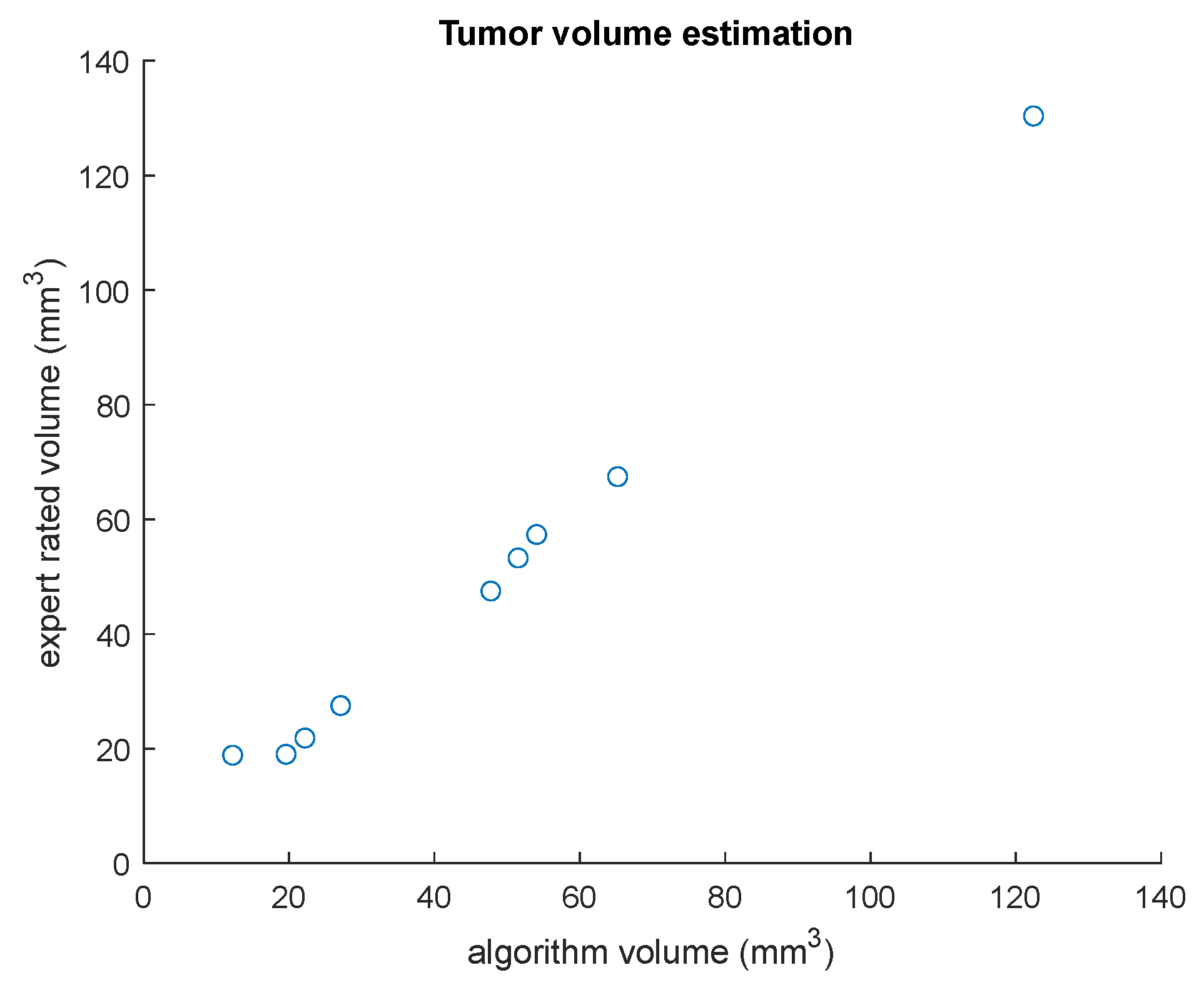
Table 5 shows the overall performance of the volume estimation algorithm. Tumor volumes of each patient estimated via the proposed system and the expert are also displayed in this table. The average percentage volume overlap fraction (Jaccard coefficient), sensitivity, and Dice similarity coefficient of the volume estimation algorithm are obtained as 89%, 91%, and 93%, respectively. It can be seen from Table 5 that the smallest Jaccard coefficient, sensitivity, and Dice similarity coefficient values are obtained in tumor volume estimation of Patient 2. In addition, graphs of tumor active core volumes obtained by the proposed algorithm and by the expert and the tumor active core volume estimation results for each patient are shown in Figure 15.
Accuracies of 89.7% and 87.6% are achieved by using the TCIA and BRATS datasets, respectively. An accuracy value of 99.0% and Dice similarity. Coefficient value of 93.0% are obtained for the proposed active core detection and volume estimation algorithm applied on the cancer imaging archive dataset. A summary of the performance of the proposed algorithm is given in Table 6. These experimental results show that the proposed approach achieved high accuracy in all tasks of the algorithm proposed for detection, segmentation, and volume estimation of brain tumors.
Table 7 displays a comparison of the proposed method and related studies in the literature. In this table, performances of the brain tumor segmentation studies by using both traditional image segmentation methods and deep learning-based methods are listed. It can be seen from this table that deep learning-based brain tumor detection methods generally provide higher accuracy than traditional segmentation methods. This comparison table also demonstrates that the proposed brain tumor detection and volume estimation method from multimodal MRI provides relatively high accuracy compared with traditional image segmentation and deep learning-based brain tumor segmentation methods.
4. Discussion
The algorithm proposed in this study is applied on multimodal brain MR images, which are FLAIR, T1-, and T1C-weighted, obtained from the TCIA and BRATS datasets. The image modality in which each brain tissue can be clearly observed differs due to differences in contrast and resolution. While the whole tumor and edema region are visible in the FLAIR modality, active core and cystic core are clearly visible in T1C modality. A multimodal analysis provides different brain tissues that can be observed in detail. The skull and non-brain regions removal process is realized by using a histogram analysis of T1 and T1C sequences, and whole tumor region segmentation is performed by using a symmetry analysis from FLAIR images. T1C images were masked with the binary image and represented the whole tumor area to narrow the ROI and to increase active core tumor segmentation success. In our study, deterioration of brain symmetry due to tumor was used as a sign, and in this way, it was possible to determine if a tumor was present in the relevant MRI slice. Therefore, in our study, the high accuracy of tumor detection based on a cross-sectional MRI slice is due to the fact that asymmetry in the brain is a distinguishing feature for tumor detection. An accuracy value of 99.0% and Dice similarity coefficient value of 93.0% are obtained in active core detection and volume estimation algorithms, respectively. The experimental results show that the proposed study provides high accuracy in brain tumor detection, segmentation, and volume estimation tasks as compared with the traditional image segmentation and deep learning-based brain tumor segmentation methods mentioned above.
In the literature, brain tumor detection studies have been performed using traditional image segmentation methods [12,14,15,16,23,25] and deep learning algorithms [26,30,31,46,47]. Ho et. al. [41] developed a method for automatic brain tumor segmentation by using level-set snakes, and they obtained a Jaccard coefficient value of 89%. Fletcher et al. [42] presented an automatic segmentation method to separate non-enhancing brain tumors from healthy tissues in MR images. Their algorithm achieved a Jaccard coefficient value of 77%. Nanda et al. [24] proposed a brain tumor classification approach using a hybrid salience-K-mean segmentation technique that depended on a deep learning method. They obtained segmentation accuracy of 96%. Chen et al. [30] proposed a brain tumor segmentation method based on a deep convolutional symmetric neural network with a Dice similarity coefficient value of 85.2%. The proposed brain tumor detection algorithm achieved accuracies of 89.7% and 87.6% by using the TCIA and BRATS datasets, respectively.
As previously mentioned, there are some studies with high accuracy in the literature. We did not implement or try their algorithms, but we used the same dataset (BRATS) in order to compare our results with those in the literature. As a result, the advantages of our study, which explain the high accuracy, are that the skull stripping stage is included in the preprocessing part and also the slices including tumor are detected before active core segmentation. In addition, the volume of the tumor is calculated after the tumor segmentation step. In our study, high success was achieved not only in the tumor detection stage, but also in the segmentation and volume estimation stages.
A limitation of the proposed study may be the execution time of the algorithm. In the current study, the execution time was computed as 258.75 s per patient for our computer specifications mentioned in the Section 3. A more powerful CPU for a computer may provide fast execution close to real-time tumor detection and volume estimation and also real-time applications in clinics. As a comparison, in a study by [48], a deep learning-based tumor segmentation algorithm with a computer configuration similar to our study was proposed. They evaluated their algorithm on the BRATS 2018 dataset by randomly choosing 48 patients’ data. They trained their network on an i7 processor, 8 GB RAM, and 4 GB NVIDIA GTX 1650 GPU. They reported that the time required to only train the given input images was almost 96 h.
One of the advantages of the proposed study is that brain tumor detection and volume estimation were performed automatically without using any user interactions and threshold values were also determined adaptively. Another advantage is that the proposed study was based on the unsupervised segmentation method, so there was no need for a very large dataset for training.
5. Conclusions
In this paper, we present a fully automated brain tumor detection, segmentation, and volume estimation method from multimodal brain MRI. The proposed algorithm was developed based on the fact that the human brain has symmetrical characteristics; however, anomalies such as a tumor in the brain cause this symmetry to be disrupted. Contributions of the current study include the following: (1) A symmetry-based method is used dynamically for large variations in tumor size, location, and shape. (2) This unsupervised tumor segmentation method eliminates the need to use a large number of MRI data required for the training phase in the supervised-based learning algorithms such as neural networks or deep learning. (3) The proposed method can accurately be used as a computer-aided system to assist physicians in surgical planning and following the growing rate of brain tumor treatment duration. (4) In addition to whole tumor segmentation, active core and cystic core segmentation and volume estimation, which are useful for the treatment plan of a patient, are possible by using this method.
Author Contributions
Conceptualization, C.F., O.E., Z.T. and O.K.; Formal analysis, C.F., Z.T. and O.K.; Investigation, O.E. and Z.T.; Methodology, C.F., O.E. and Z.T.; Software, C.F.; Supervision, O.E. and Z.T.; Validation, O.E., Z.T. and O.K.; Visualization, C.F. and O.K.; Writing—original draft, C.F. and Z.T.; Writing—review and editing, O.E. and Z.T. All authors have read and agreed to the published version of the manuscript.
Funding
This research received no external funding.
Institutional Review Board Statement
This study was conducted in accordance with the Declaration of Helsinki, and approved by the Ethics Committee of Ankara University Faculty of Medicine Human Research Ethics Committee (approval code i5-225-19, approval date, 14 November 2019).
Data Availability Statement
Brain MRI dataset is publicaly available at https://www.cancerimagingarchive.net/, accessed on 21 April 2022.
Conflicts of Interest
The authors declare no conflict of interest.
References
- Villanueva-Meyer, J.E.; Mabray, M.C.; Cha, S. Current clinical brain tumor imaging. Neurosurgery 2017, 81, 397–415. [Google Scholar] [CrossRef] [Green Version]
- Nabizadeh, N.; Kubat, M. Brain tumors detection and segmentation in MR images: Gabor wavelet vs. statistical features. Comput. Electr. Eng. 2015, 45, 286–301. [Google Scholar] [CrossRef]
- Yang, D. Standardized MRI assessment of high-grade glioma response: A review of the essential elements and pitfalls of the RANO criteria. Neuro-Oncol. Pract. 2016, 3, 59–67. [Google Scholar] [CrossRef] [PubMed] [Green Version]
- Leao, D.J.; Craig, P.G.; Godoy, L.F.; Leite, C.C.; Policeni, B. Response assessment in neuro-oncology criteria for gliomas: Practical approach using conventional and advanced techniques. Am. J. Neuroradiol. 2020, 41, 10–20. [Google Scholar] [CrossRef] [PubMed]
- Dou, W.; Ruan, S.; Chen, Y.; Bloyet, D.; Constans, J.M. A framework of fuzzy information fusion for the segmentation. Image Vis. Comput. 2007, 25, 164–171. [Google Scholar] [CrossRef]
- Verma, R.; Zacharaki, E.; Ou, Y.; Davatzikos, C. Multiparametric Tissue Characterization of Brain Neoplasms and Their Recurrence Using Pattern Classification of MR Images. Acad. Radiol. 2008, 15, 966–977. [Google Scholar] [CrossRef] [Green Version]
- Joe, B.N.; Fukui, M.B.; Meltzer, C.C.; Huang, Q.S.; Day, R.S.; Greer, P.J.; Bozik, M.E. Brain tumor volume measurement: Comparison of manual and semiautomated methods. Radiology 1999, 212, 811–816. [Google Scholar] [CrossRef]
- Dempsey, M.F.; Condon, B.R.; Hadley, D.M. Measurement of tumor “size” in recurrent malignant glioma: 1D, 2D, or 3D? Am. J. Neuroradiol. 2005, 26, 770–776. [Google Scholar]
- Meier, R.; Knecht, U.; Loosli, T.; Bauer, S.; Slotboom, J.; Wiest, R.; Reyes, M. Clinical evaluation of a fully-automatic segmentation method for longitudinal brain tumor volumetry. Sci. Rep. 2016, 6, 23376. [Google Scholar] [CrossRef] [Green Version]
- Barzegar, Z.; Jamzad, M. Fully automated glioma tumour segmentation using anatomical symmetry plane detection in multimodal brain MRI. IET Comput. Vis. 2021, 15, 463–473. [Google Scholar] [CrossRef]
- Harati, V.; Khayati, R.; Farzan, A. Fully automated tumor segmentation based on improved fuzzy connectedness algorithm in brain MR images. Comput. Biol. Med. 2011, 41, 483–492. [Google Scholar] [CrossRef] [PubMed]
- Dvořák, P.; Kropatsch, W.G.; Bartušek, K. Automatic brain tumor detection in t2-weighted magnetic resonance images. Meas. Sci. Rev. 2013, 13, 223–230. [Google Scholar] [CrossRef] [Green Version]
- Latif, G.; Ben Brahim, G.; Iskandar, D.N.F.A.; Bashar, A.; Alghazo, J. Glioma Tumors’ classification using deep-neural-network-based features with SVM classifier. Diagnostics 2022, 12, 1018. [Google Scholar] [CrossRef] [PubMed]
- Ogretmenoglu, C.; Erogul, O.; Telatar, Z.; Guler, E.R.; Yildirim, F. Brain tumor detection and volume estimation via MR imaging. J. Biotechnol. 2015, 208, S15. [Google Scholar] [CrossRef]
- Ogretmenoglu, C.; Telatar, Z.; Erogul, O. MR Image Segmentation and Symmetry Analysis for Detection of Brain Tumor. J. Biotechnol. 2016, 231, 9. [Google Scholar] [CrossRef]
- Fiçici, C.Ö.; Eroğul, O.; Telatar, Z. Fully automated brain tumor segmentation and volume estimation based on symmetry analysis in MR images. In CMBEBIH 2017: Proceedings of the International Conference on Medical and Biological Engineering; Springer: Singapore, 2017; pp. 53–60. [Google Scholar] [CrossRef]
- Clark, M.C.; Hall, L.O.; Goldgof, D.B.; Velthuizen, R.; Murtagh, F.R.; Silbiger, M.S. Automatic Tumor Segmentation Using knowledge-based techniques. IEEE Trans. Med. Imaging 1998, 17, 187–201. [Google Scholar] [CrossRef] [Green Version]
- Nie, J.; Xue, Z.; Liu, T.; Young, G.S.; Setayesh, K.; Guo, L.; Wong, S.T. Automated Brain Tumor Segmentation Using Spatial Accuracy-Weighted Hidden Markov Random Field. Comput. Med. Imaging Graph. 2009, 33, 431–441. [Google Scholar] [CrossRef] [Green Version]
- Kaus, M.R.; Warfield, S.K.; Nabavi, A.; Black, P.M.; Jolesz, F.A.; Kikinis, R. Automated Segmentation of MR Images of Brain Tumors. Radiology 2001, 218, 586–591. [Google Scholar] [CrossRef] [Green Version]
- Prastawa, M.; Bullitt, E.; Ho, S.; Gerig, G. A brain tumor segmentation framework based on outlier detection. Med. Image Anal. 2004, 8, 275–283. [Google Scholar] [CrossRef]
- Wang, T.; Cheng, I.; Basu, A. Fluid vector flow and applications in brain tumor segmentation. IEEE Trans. Biomed. Eng. 2009, 56, 781–789. [Google Scholar] [CrossRef]
- Khotanlou, H.; Colliot, O.; Atif, J.; Bloch, I. 3D brain tumor segmentation in MRI using fuzzy classification, symmetry analysis and spatially constrained deformable models. Fuzzy Sets Syst. 2009, 160, 1457–1473. [Google Scholar] [CrossRef] [Green Version]
- Kermi, A.; Andjouh, K.; Zidane, F. Fully automated brain tumour segmentation system in 3D-MRI using symmetry analysis of brain and level sets. IET Image Process. 2018, 12, 1964–1971. [Google Scholar] [CrossRef]
- Nanda, A.; Barik, R.C.; Bakshi, S. SSO-RBNN driven brain tumor classification with Saliency-K-means segmentation technique. Biomed. Signal Process. Control 2023, 81, 104356. [Google Scholar] [CrossRef]
- Khosravanian, A.; Rahmanimanesh, M.; Keshavarzi, P.; Mozaffari, S.; Kazemi, K. Level set method for automated 3D brain tumor segmentation using symmetry analysis and kernel induced fuzzy clustering. Multimed. Tools Appl. 2022, 81, 21719–21740. [Google Scholar] [CrossRef]
- Wu, X.; Bi, L.; Fulham, M.; Feng, D.D.; Zhou, L.; Kim, J. Unsupervised brain tumor segmentation using a symmetric-driven adversarial network. Neurocomputing 2021, 455, 242–254. [Google Scholar] [CrossRef]
- Bertamini, M.; Makin, A.D. Brain activity in response to visual symmetry. Symmetry 2014, 6, 975–996. [Google Scholar] [CrossRef] [Green Version]
- Corballis, M.C. Bilaterally symmetrical: To be or not to be? Symmetry 2020, 12, 326. [Google Scholar] [CrossRef] [Green Version]
- Khalil, H.A.; Darwish, S.; Ibrahim, Y.M.; Hassan, O.F. 3D-MRI brain tumor detection model using modified version of level set segmentation based on dragonfly algorithm. Symmetry 2020, 12, 1256. [Google Scholar] [CrossRef]
- Chen, H.; Qin, Z.; Ding, Y.; Tian, L.; Qin, Z. Brain tumor segmentation with deep convolutional symmetric neural network. Neurocomputing 2020, 392, 305–313. [Google Scholar] [CrossRef]
- Athisayamani, S.; Antonyswamy, R.S.; Sarveshwaran, V.; Almeshari, M.; Alzamil, Y.; Ravi, V. Feature Extraction Using a Residual Deep Convolutional Neural Network (ResNet-152) and Optimized Feature Dimension Reduction for MRI Brain Tumor Classification. Diagnostics 2023, 13, 668. [Google Scholar] [CrossRef]
- Pedada, K.R.; Rao, B.; Patro, K.K.; Allam, J.P.; Jamjoom, M.M.; Samee, N.A. A novel approach for brain tumour detection using deep learning based technique. Biomed. Signal Process. Control 2023, 82, 104549. [Google Scholar] [CrossRef]
- Alshammari, S.; Al-Sawalha, M.M.; Shah, R. Approximate Analytical Methods for a Fractional-Order Nonlinear System of Jaulent–Miodek Equation with Energy-Dependent Schrödinger Potential. Fractal Fract. 2023, 7, 140. [Google Scholar] [CrossRef]
- Shah, N.A.; Hamed, Y.S.; Abualnaja, K.M.; Chung, J.D.; Shah, R.; Khan, A. A Comparative Analysis of Fractional-Order Kaup–Kupershmidt Equation within Different Operators. Symmetry 2022, 14, 986. [Google Scholar] [CrossRef]
- Al-Sawalha, M.M.; Ababneh, O.Y.; Shah, R.; Shah, N.A.; Nonlaopon, K. Combination of Laplace transform and residual power series techniques of special fractional-order non-linear partial differential equations. AIMS Math. 2023, 8, 5266–5280. [Google Scholar] [CrossRef]
- The Cancer Imaging Archive (TCIA). 2023. Available online: https://www.cancerimagingarchive.net/ (accessed on 21 April 2022).
- Menze, B.H.; Jakab, A.; Bauer, S.; Kalpathy-Cramer, J.; Farahani, K.; Kirby, J.; Burren, Y.; Porz, N.; Slotboom, J.; Wiest, R.; et al. The Multimodal Brain Tumor Image Segmentation Benchmark (BRATS). IEEE Trans. Med. Imaging 2015, 34, 1993–2024. [Google Scholar] [CrossRef] [PubMed]
- Bakas, S.; Akbari, H.; Sotiras, A.; Bilello, M.; Rozycki, M.; Kirby, J.S.; Freymann, J.B.; Farahani, K.; Davatzikos, C. Advancing The Cancer Genome Atlas glioma MRI collections with expert segmentation labels and radiomic features. Nat. Sci. Data 2017, 4, 170117. [Google Scholar] [CrossRef] [PubMed] [Green Version]
- Bakas, S.; Reyes, M.; Jakab, A.; Bauer, S.; Rempfler, M.; Crimi, A.; Shinohara, R.T.; Berger, C.; Ha, S.M.; Rozycki, M.; et al. Identifying the Best Machine Learning Algorithms for Brain Tumor Segmentation, Progression Assessment, and Overall Survival Prediction in the BRATS Challenge. arXiv 2018, arXiv:1811.02629. [Google Scholar] [CrossRef]
- Chuang, K.-S.; Tzeng, H.-L.; Chen, S.; Wu, J.; Chen, T.-J. Fuzzy c-means clustering with spatial information for image segmentation. Comput. Med. Imaging Graph. 2006, 30, 9–15. [Google Scholar] [CrossRef] [Green Version]
- Ho, S.; Bullitt, E.; Gerig, G. Level Set Evolution with Region Competition: Automatic 3-D segmentation of brain tumors. In Proceedings of the 16th International Conference on Pattern Recognition, Quebec City, QC, Canada, 11–15 August 2002. [Google Scholar]
- Fletcher-Heath, L.M.; Hall, L.O.; Goldgof, D.B.; Murtagh, F.R. Automatic segmentation of non-enhancing brain tumors in magnetic resonance images. Artif. Intell. Med. 2001, 21, 43–63. [Google Scholar] [CrossRef] [Green Version]
- Zhang, J.; Ma, K.-K.; Er, M.H.; Chong, V. Tumor segmentation from magnetic resonance imaging by learning via one-class support vector machine. In Proceedings of the International Workshop on Advanced Imaging Technology, Chengdu, China, 12–13 January 2004. [Google Scholar]
- Corso, J.J.; Sharon, E.; Dube, S.; El-Saden, S.; Sinha, U.; Yuille, A. Efficient Multilevel Brain Tumor Segmentation with Integrated Bayesian Model Classification. Trans. Med. Imaging 2008, 27, 629–640. [Google Scholar] [CrossRef] [Green Version]
- Prastawa, M.; Bullitt, E.; Moon, N.; Leemput, K.V.; Gerig, G. Automatic brain tumor segmentation by subject specific modification of atlas priors. Acad. Radiol. 2004, 10, 1341–1348. [Google Scholar] [CrossRef] [PubMed] [Green Version]
- Mahmoud, A.; Awad, N.A.; Alsubaie, N.; Ansarullah, S.I.; Alqahtani, M.S.; Abbas, M.; Usman, M.; Soufiene, B.O.; Saber, A. Advanced Deep Learning Approaches for Accurate Brain Tumor Classification in Medical Imaging. Symmetry 2023, 15, 571. [Google Scholar] [CrossRef]
- Mahmud, M.I.; Mamun, M.; Abdelgawad, A.A. Deep Analysis of Brain Tumor Detection from MR Images Using Deep Learning Networks. Algorithms 2023, 16, 176. [Google Scholar] [CrossRef]
- Battalapalli, D.; Rao, B.P.; Yogeeswari, P.; Kesavadas, C.; Rajagopalan, V. An optimal brain tumor segmentation algorithm for clinical MRI dataset with low resolution and non-contiguous slices. BMC Med. Imaging 2022, 22, 89. [Google Scholar] [CrossRef]
Figure 1.
The proposed brain tumor detection and volume estimation algorithm flowchart for a patient.
Figure 1.
The proposed brain tumor detection and volume estimation algorithm flowchart for a patient.

Figure 2.
(a) T1 image; (b) T1C image; (c) FLAIR image; (d) median-filtered T1 image; (e) median-filtered T1C image; (f) median-filtered FLAIR image.
Figure 2.
(a) T1 image; (b) T1C image; (c) FLAIR image; (d) median-filtered T1 image; (e) median-filtered T1C image; (f) median-filtered FLAIR image.

Figure 3.
Histogram analysis for skull stripping.

Figure 4.
Skull stripping block diagram.

Figure 5.
(a) T1 image; (b) skull stripping mask; (c) masked T1C image; (d) masked FLAIR image.

Figure 6.
(a) Skull-stripped FLAIR image and symmetry axis; (b) separating FLAIR image into two equal halves; (c) fuzzy c-means clustering result.
Figure 6.
(a) Skull-stripped FLAIR image and symmetry axis; (b) separating FLAIR image into two equal halves; (c) fuzzy c-means clustering result.

Figure 7.
Framework of the symmetry analysis.

Figure 8.
Framework of symmetry analysis: (a) Area difference; (b) mean difference; (c) BC asymmetry score graphs of a patient (Example 1).
Figure 8.
Framework of symmetry analysis: (a) Area difference; (b) mean difference; (c) BC asymmetry score graphs of a patient (Example 1).

Figure 9.
Framework of symmetry analysis: (a) Area difference; (b) mean difference; (c) BC asymmetry score graphs of a patient (Example 2).
Figure 9.
Framework of symmetry analysis: (a) Area difference; (b) mean difference; (c) BC asymmetry score graphs of a patient (Example 2).

Figure 10.
Whole tumor segmentation flowchart.

Figure 11.
Enhancing and necrotic core segmentation flowchart.

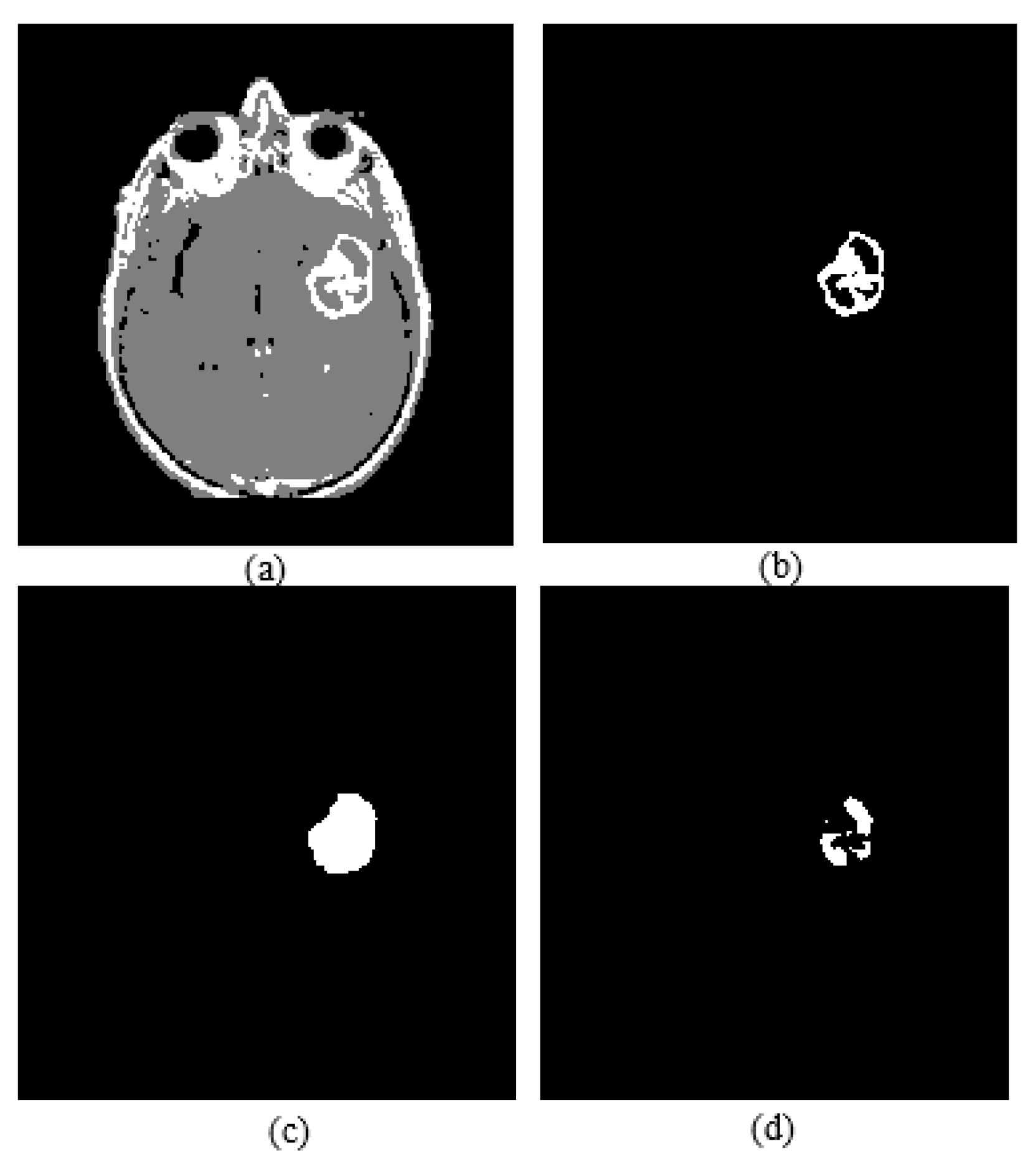
Figure 12.
(a) T1C image; (b) fuzzy c-means clustering result; (c) binary image including active core; (d) skull stripping mask; (e) whole tumor mask; (f) enhancing tumor.
Figure 12.
(a) T1C image; (b) fuzzy c-means clustering result; (c) binary image including active core; (d) skull stripping mask; (e) whole tumor mask; (f) enhancing tumor.

Figure 13.
(a) FCM clustering result of a T1C image; (b) enhancing tumor; (c) image closing result; (d) necrotic core.
Figure 13.
(a) FCM clustering result of a T1C image; (b) enhancing tumor; (c) image closing result; (d) necrotic core.

Figure 14.
Graph of tumor active core detection results for each patient.

Figure 15.
Graph of tumor active core volumes obtained by the proposed algorithm and by the expert for all patients.
Figure 15.
Graph of tumor active core volumes obtained by the proposed algorithm and by the expert for all patients.


Table 1.
Results of the detection of the slices containing tumor active core algorithm.
| Patient | Number of Slices | Number of Slices Containing Tumor | TP | FN | FP | TN |
|---|---|---|---|---|---|---|
| 1 | 49 | 18 | 17 | 1 | 0 | 31 |
| 2 | 54 | 10 | 8 | 2 | 0 | 44 |
| 3 | 54 | 16 | 16 | 0 | 0 | 38 |
| 4 | 55 | 9 | 9 | 0 | 0 | 46 |
| 5 | 53 | 22 | 20 | 1 | 0 | 32 |
| 6 | 51 | 11 | 11 | 0 | 0 | 40 |
| 7 | 55 | 9 | 9 | 0 | 0 | 46 |
| 8 | 58 | 14 | 14 | 0 | 0 | 44 |
| 9 | 50 | 16 | 16 | 0 | 0 | 34 |
| Total | 479 | 125 | 120 | 4 | 0 | 355 |
Table 2.
Tumor active core detection results.
| Patient | Sensitivity (%) | Specificity (%) | Accuracy (%) |
|---|---|---|---|
| 1 | 94 | 100 | 98 |
| 2 | 80 | 100 | 96 |
| 3 | 100 | 100 | 100 |
| 4 | 100 | 100 | 100 |
| 5 | 95 | 100 | 98 |
| 6 | 100 | 100 | 100 |
| 7 | 100 | 100 | 100 |
| 8 | 100 | 100 | 100 |
| 9 | 100 | 100 | 100 |
| Average | 97 | 100 | 99 |
Table 3.
Results of the tumor active core volume estimation algorithm for a patient (Example 1).
| MR Slice | Area Calculated by the Algorithm (mm2) | Area Calculated by the Expert (mm2) | Jaccard Coefficient (%) | Sensitivity (%) | Dice Similarity Coefficient (%) |
|---|---|---|---|---|---|
| 16 | 470.27 | 464.11 | 99 | 100 | 99 |
| 17 | 583.66 | 574.87 | 98 | 100 | 99 |
| 18 | 660.13 | 669.8 | 99 | 99 | 99 |
| 19 | 697.05 | 707.6 | 99 | 99 | 99 |
| 20 | 617.94 | 634.64 | 97 | 97 | 99 |
| 21 | 857.03 | 807.8 | 93 | 100 | 97 |
| 22 | 1034.6 | 1086.4 | 93 | 94 | 96 |
| 23 | 1271 | 1298.3 | 97 | 97 | 99 |
| 24 | 1566.4 | 1523.3 | 97 | 100 | 98 |
| 25 | 1385.3 | 1422.2 | 97 | 97 | 99 |
| 26 | 1560.2 | 1584.8 | 98 | 98 | 99 |
| 27 | 1620.9 | 1600 | 99 | 100 | 99 |
| 28 | 1657.8 | 1705.3 | 97 | 97 | 99 |
| 29 | 0 | 1476.7 | 0 | 0 | 99 |
| 30 | 1679.8 | 1713.2 | 98 | 98 | 99 |
| 31 | 1858.2 | 1799.3 | 97 | 100 | 98 |
| 32 | 1714.1 | 1743.1 | 98 | 98 | 99 |
| 33 | 1630.1 | 1578.7 | 97 | 100 | 98 |
| 34 | 1050 | 1025.8 | 98 | 100 | 99 |
| 35 | 705.84 | 701.44 | 97 | 99 | 99 |
| 36 | 428.07 | 430.71 | 97 | 98 | 98 |
| 37 | 173.16 | 175.8 | 99 | 99 | 99 |
Table 4.
Results of the tumor active core area calculation for a patient (Example 2).
| MR Slice | Area Calculated by the Algorithm (mm2) | Area Calculated by the Expert (mm2) | Jaccard Coefficient (%) | Sensitivity (%) | Dice Similarity Coefficient (%) |
|---|---|---|---|---|---|
| 21 | 627.61 | 614.42 | 98 | 100 | 99 |
| 22 | 959.87 | 958.99 | 100 | 100 | 100 |
| 23 | 1052.2 | 1030.2 | 98 | 100 | 99 |
| 24 | 714.63 | 703.2 | 98 | 100 | 99 |
| 25 | 846.48 | 842.08 | 99 | 100 | 100 |
| 26 | 719.02 | 756.46 | 95 | 95 | 97 |
| 27 | 936.14 | 932.62 | 100 | 100 | 100 |
| 28 | 738.36 | 728.69 | 99 | 100 | 99 |
| 29 | 890.43 | 902.73 | 99 | 99 | 99 |
| 30 | 731.33 | 740.12 | 99 | 99 | 99 |
| 31 | 515.97 | 478.18 | 93 | 100 | 96 |
| 32 | 174.04 | 172.28 | 99 | 100 | 99 |
| 33 | 43.95 | 47.47 | 93 | 93 | 96 |
| 34 | 105.48 | 99.33 | 94 | 100 | 97 |
Table 5.
Performance of the tumor volume estimation algorithm.
| Patient | Volume Estimated by the Algorithm (mm2) | Volume Estimated by the Expert (mm2) | Jaccard Coefficient (%) | Sensitivity (%) | Dice Similarity Coefficient (%) |
|---|---|---|---|---|---|
| 1 | 65,212 | 67,442 | 82 | 86 | 88 |
| 2 | 12,250 | 18,838 | 67 | 68 | 72 |
| 3 | 51,518 | 53,257 | 87 | 92 | 93 |
| 4 | 19,577 | 19,011 | 94 | 98 | 97 |
| 5 | 122,415 | 130,393 | 93 | 94 | 99 |
| 6 | 27,105 | 27,488 | 92 | 94 | 96 |
| 7 | 22,192 | 21,832 | 96 | 98 | 98 |
| 8 | 47,759 | 47,502 | 97 | 99 | 99 |
| 9 | 54,073 | 57,345 | 93 | 94 | 96 |
| Average | 89 | 91 | 93 |
Table 6.
Summary of the performance of the proposed algorithm.
| Algorithm | Dataset | Number of Patients (Number of MRI Slices) | Accuracy (%) |
|---|---|---|---|
| Whole tumor detection | TCIA | 10 (529) | 89.7 |
| BRATS | 11 (1705) | 87.6 | |
| Active core detection | TCIA | 9 (479) | 99.0 |
| Active core volume estimation | TCIA | 9 (479) | 93.0 (Dice similarity coefficient) |
Table 7.
Comparison of the proposed volume estimation method and alternative methods in the literature.
Table 7.
Comparison of the proposed volume estimation method and alternative methods in the literature.
| Author | Dataset | MRI Modality | Approach | Results (%) |
|---|---|---|---|---|
| Ho et al. [41] | Their study database | T1 and T1C | Level set evaluation; snake | Jaccard coefficient: 89 |
| Prastawa et al. [20] | Their study database | T2 | Level-set evaluation; outlier detection | Jaccard coefficient: 77 |
| Fletcher et al. [42] | Their study database | T1, T2, and Proton Density (PD) | Unsupervised fuzzy clustering, knowledge-based system | Jaccard coefficient: 74 |
| Zhang et al. [43] | Their study database | T2 | Support vector machine (SVM) | Jaccard coefficient: 72 |
| Clarc et al. [17] | Their study database | T1, T2, and Proton Density (PD) | Knowledge-based (KB) segmentation, histogram analysis | Jaccard coefficient: 70 |
| Corso et al. [44] | Their study database | T1, T1C, FLAIR, and T2 | Multilevel Bayesian segmentation | Jaccard coefficient: 69 |
| Prastawa et al. [45] | Their study database | T1, T1C, and T2 | Expectation-maximization (EM) method guided by a spatial probabilistic atlas | Jaccard coefficient: 59 |
| Nanda et al. [24] | Kaggle (Dataset-1), BRATS (Dataset-2) | FLAIR | Hybrid salience-K-mean segmentation | Segmentation accuracy (Dataset-1): 96 (Dataset-2): 92 |
| Pedada et al. [32] | BRATS-2017 (Dataset-1) BRATS-2018 (Dataset-2) | T1, T1C, and FLAIR | U-Net model | Segmentation accuracy (Dataset-1): 93.4 (Dataset-2): 92.2 |
| Athisayamani et al. [31] | Figshare (Dataset-1) BRATS 2019 (Dataset-2) MICCAI BRATS (Dataset-3) | (Information does not exist in the paper.) | Residual deep convolutional neural network (ResNet-152) and the Canny Mayfly algorithm | Segmentation accuracy (Dataset-1): 97 (Dataset-2): 98 (Dataset-3): 99 |
| Khosravanian et al. [25] | BRATS 2017 | FLAIR | Fuzzy kernel level set (FKLS) for 3D brain tumor segmentation | Dice: 97.62% Jaccard: 95.41% Sensitivity: 98.79% Specificity: 99.85% |
| Wu et al. [26] | BRATS 2012 BRATS 2018 | T2 | Symmetric-driven adversarial network | Dice: 64.6% Sensitivity: 80.2% Specificity: 70.1% |
| Barzegar et al. [10] | BRATS 2015 BRATS 2017 BRATS 2019 | T1, T1C, FLAIR, and T2 | Symmetry plane detection followed by similarity comparison | Segmentation accuracy (Dataset-1): Dice score: 86.3 Jaccard: 80.5 (Dataset-2): Dice score: 92.7 Jaccard: 82.3 (Dataset-3): Dice score: 91.3 Jaccard: 84.1 |
| Chen et al. [30] | BRATS 2015 | T1, T1c, T2, and Flair | Deep convolutional neural network which combines symmetry | Dice similarity coefficient: 85.2 |
| Khalil et al. [29] | BRATS 2017 | T1 or T1c or T2 or Flair | Level set segmentation based on the dragonfly algorithm | Accuracy: 98.2 Recall: 95.13 Precision: 93.21 |
| Kermi et al. [23] | BRATS 2017 | FLAIR or T2 | Symmetry analysis based on the fast bounding box, region growing, and geodesic level-set methods | Sensitivity: 81.59 (T2) 89.01 (FLAIR) Kappa: 76.82 (T2) 83.04 (FLAIR) |
| Proposed Method | Cancer imaging archive | T1, T1C, and FLAIR | Histogram Analysis, Adaptive thresholding, Symmetry Analysis, FCM | Accuracy: 89.7 (whole tumor detection) Accuracy: 99 (active core detection) Sensitivity: 97 (active core detection) Jaccard coefficient: 89 (active core volume estimation) Sensitivity: 91 (active core volume estimation) Dice similarity coefficient: 93 (active core volume estimation) |
| BRATS 2018 | Accuracy: 87.6 (whole tumor detection) |
Disclaimer/Publisher’s Note: The statements, opinions and data contained in all publications are solely those of the individual author(s) and contributor(s) and not of MDPI and/or the editor(s). MDPI and/or the editor(s) disclaim responsibility for any injury to people or property resulting from any ideas, methods, instructions or products referred to in the content. |
© 2023 by the authors. Licensee MDPI, Basel, Switzerland. This article is an open access article distributed under the terms and conditions of the Creative Commons Attribution (CC BY) license (https://creativecommons.org/licenses/by/4.0/).
Share and Cite
MDPI and ACS Style
Ficici, C.; Erogul, O.; Telatar, Z.; Kocak, O. Automatic Brain Tumor Detection and Volume Estimation in Multimodal MRI Scans via a Symmetry Analysis. Symmetry 2023, 15, 1586. https://doi.org/10.3390/sym15081586
AMA Style
Ficici C, Erogul O, Telatar Z, Kocak O. Automatic Brain Tumor Detection and Volume Estimation in Multimodal MRI Scans via a Symmetry Analysis. Symmetry. 2023; 15(8):1586. https://doi.org/10.3390/sym15081586
Chicago/Turabian StyleFicici, Cansel, Osman Erogul, Ziya Telatar, and Onur Kocak. 2023. "Automatic Brain Tumor Detection and Volume Estimation in Multimodal MRI Scans via a Symmetry Analysis" Symmetry 15, no. 8: 1586. https://doi.org/10.3390/sym15081586
Note that from the first issue of 2016, this journal uses article numbers instead of page numbers. See further details here.