Symmetric Strange Attractors: A Review of Symmetry and Conditional Symmetry

Abstract

A comprehensive review of symmetry and conditional symmetry is made from the core conception of symmetry and conditional symmetry. For a dynamical system, the structure of symmetry means its robustness against the polarity change of some of the system variables. Symmetric systems typically show symmetrical dynamics, and even when the symmetry is broken, symmetric pairs of coexisting attractors are born, annotating the symmetry in another way. The polarity balance can be recovered through combinations of the polarity reversal of system variables, and furthermore, it can also be restored by the offset boosting of some of the system variables if the variables lead to the polarity reversal of their functions. In this case, conditional symmetry is constructed, giving a chance for a dynamical system outputting coexisting attractors. Symmetric strange attractors typically represent the flexible polarity reversal of some of the system variables, which brings more alternatives of chaotic signals and more convenience for chaos application. Symmetric and conditionally symmetric coexisting attractors can also be found in memristive systems and circuits. Therefore, symmetric chaotic systems and systems with conditional symmetry provide sufficient system options for chaos-based applications.

1. Introduction

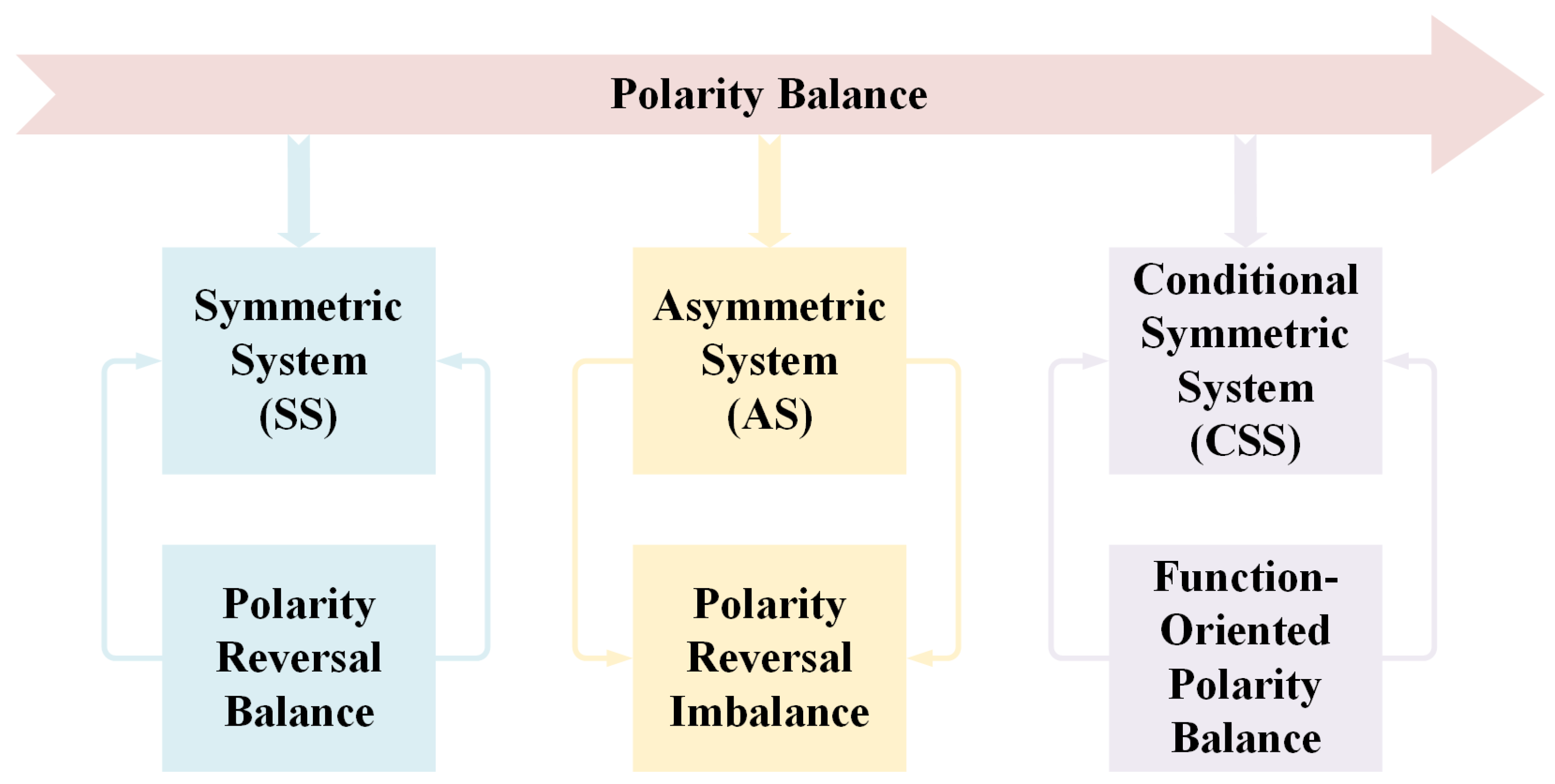
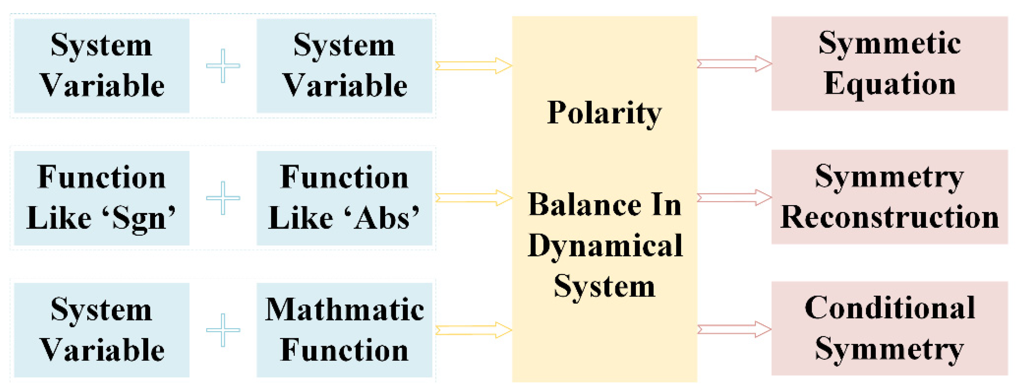
For a dynamical system, the structure of it typically determines the solution feature. From the view of symmetry, the polarity reversal of some of the system variables may not influence the solution because of the symmetric structure. The Lorenz system [1], Chen system [2] and Chua circuit [3] are all examples of such structures. In addition, symmetric systems have aesthetic characteristics; a symmetric system seems to be more robust according to the polarity revision from a variable. Symmetric chaotic systems do not reject the specific feedback of a hyperbolic sinusoidal function [4]. A cyclic symmetric conservative chaotic system can also be constructed with offset boosting [5]. Rotational symmetry has its specific detection method [6,7], and symmetry breaking exists commonly in dynamical systems [8]. When some of the variables are polarity reversed, the system outputs the symmetric attractor without any influence or even gives symmetric pairs of attractors. As found, symmetry-breaking, amplitude control and constant Lyapunov exponents may coexist in a single system [9]. A hyperchaotic memcapacitor oscillator may have infinite equilibria and coexisting attractors without losing symmetry [10]. Various synchronization phenomena can be found in a bidirectionally coupled double scroll circuit [11]. An infinite-dimensional stochastic system may still own the symmetric structure [12], and multistable dynamics and control can be realized in a symmetric 4D memristive system [13]. But for asymmetric systems, any polarity disturbance will destroy the solution. From this view, symmetric systems have stronger stability. More changes in variables in a dynamical system do not necessarily bring more instability. However, in a conditional symmetric system, the polarity reversal could be consumed by offset boosting in some of the dimensions. As shown in Figure 1, here, polarity balance is broken and recovered among those different topologies of the system structure. We can see that in a symmetric system the polarity balance is recovered by the polarity reversal of some of the system variables. Typically, an asymmetric system will lose polarity balance when some of the system variables are polarity reversed. But function-oriented polarity balance can be obtained in symmetric systems and asymmetric systems, which is called as conditional symmetry.

The issue of symmetry in fact widely appears in various systems of different fields, such as in mechanical systems [14,15,16], economic systems [17,18], chemical systems [19,20,21], neuron systems [22,23], ecosystems [24,25], electronic systems [26,27], physical systems [28,29], geographic systems [30,31] and environmental systems [32,33]. Polarity reversal means various patterns of evolution and indicates different physical properties. Specifically, in electronic engineering, symmetric evolution implies the polarity reversal of associated system variables and correspondingly means that a single system can output multiple electronic signals by selecting different initial conditions. Methods of qualitative theory in nonlinear dynamics also reveal an associated principle hidden in symmetry [34]. A symmetric system typically exhibits specifical bifurcation [35], and more strikingly, this topology can also be revised to include multiple-wing attractors [36,37,38]. Some symmetric systems have an infinite number of periodic orbits or aperiodic trajectories [39,40,41]. The diverse and flexible evolutionary attributes of symmetric chaotic systems give them extensive application value in various fields, such as image encryption [42,43,44,45], speech encryption [46,47,48] and random number generating [49,50].

Extensive work indicates that stronger performance is achieved by the specific symmetric topology. Furthermore, toward this direction, symmetric chaotic systems can be rebuilt, and even partially symmetric systems marked by conditional symmetry can be obtained based on offset boosting of a system variable. In this work, our goal is to demonstrate those coexisting attractors hidden in the specific topology of symmetry. We summarize those regimes of symmetric systems that host coexisting symmetric pairs of attractors along with those symmetric attractors in Section 2. In Section 3, the mechanism hidden in the offset boosting for system symmetrization is disclosed and reviewed. Symmetric pairs of coexisting attractors are produced based on this approach with desired distances. In Section 4, offset boosting is applied for constructing chaotic systems with conditional symmetry under various structures, where coexisting conditional symmetric pairs of attractors are obtained. Section 5 reviews symmetry and elegance in simple chaotic circuits, which are also prone to output coexisting symmetric pairs of attractors under some specific conditions. Thereafter, a concise conclusion is offered in the last section.

2. Symmetric Strange Attractors and Symmetric Pairs of Coexisting Attractors

2.1. Various Regimes of Symmetry

The topology of a symmetric system means a unique structure that shows the invariance of the system under some transformation of polarity reversal. And furthermore, when the symmetry is broken, normally, a pair of coexisting asymmetric solutions may appear, sometimes along with some symmetric solutions, and the system outputs coexisting asymmetric and symmetric strange attractors. The fundamental striction is polarity balance in a dynamical system. For a dynamical equation, any transformation should obey some basic laws, and the basic rule is polarity balance. Not all of the systems can resist polarity transformation; many lose polarity balance when any of the state variables are polarity reversed. However, some of the systems named symmetric ones can recover the polarity balance when some of the dimensions are polarity reversed. Furthermore, the polarity balance of a dynamical system can be obtained by any operation such as offset boosting from any of the variables for the reason that the polarity reversal of any of the variables can also be induced by the offset boosting of any of the variables. We know that the derivative of $-x_{i_h}$ gives a definitely negative polarity on the left-hand side in the dimension of i_h; meanwhile a negative sign on the right-hand side could be obtained by many approaches, including the offset boosting of a variable or from a function.

We know that some of the variables being polarity reversed will not break the polarity balance in a symmetric dynamical system; at the same time, an asymmetric one will lose its polarity balance. For example, for a dynamical system $\dot{X}=F\left(X\right)=\left(f_1\right(X),f_2(X),\dots ,f_N(X\left)\right)$ ($X=\left(x_1,x_2,\dots ,x_N\right))$, if we take the variable substitution as: $u_{i_1}={-x}_{i_1},u_{i_2}={-x}_{i_2},\cdots ,u_{i_k}={-x}_{i_k},u_i=x_i$, (here, $1\le i_1,\cdots ,i_k\le N$, $i_1,\cdots ,i_k$ are not identical, $i\in \left\{1,2,\dots ,N\right\}\backslash \{i_1,\cdots ,i_k\}$) satisfying $\dot{U}=F\left(U\right)$ ($U=\left(u_1,u_2,\dots ,u_N\right))$, then the system $\dot{X}=F\left(X\right)$ ($X=\left(x_1,x_2,\dots ,x_N\right))$ can be called a symmetric system. For a three-dimensional dynamical system, $\dot{X}=F\left(X\right)$ ($X=\left(x_1,x_2,x_3\right))$, if $x_{i_0}={-u}_{i_0}(i_0\in \{1,2,3\left\}\right)$ is subject to the same governing equation, the system is named a reflection-symmetric system. If $x_{i_0}={-u}_{i_0},x_{j_0}={-u}_{j_0}(i_0,j_0\in \left\{1,2,3\right\},i_0\ne j_0)$ does not influence the governing equation, the system exhibits rotational symmetry, and if $x_1={-u}_1,x_2={-u}_2,x_3={-u}_3$ leading to the same governing equation, the system exhibits inversion symmetry. All kinds of symmetric systems could hatch coexisting attractors when the symmetry is broken, where coexisting attractors are located in those independent sub-phase spaces. In the following, we see that those coexisting attractors could be a symmetric pair of attractors or combined with a symmetric one.

2.2. Multiple Modes of Coexisting Attractors in a Symmetric System

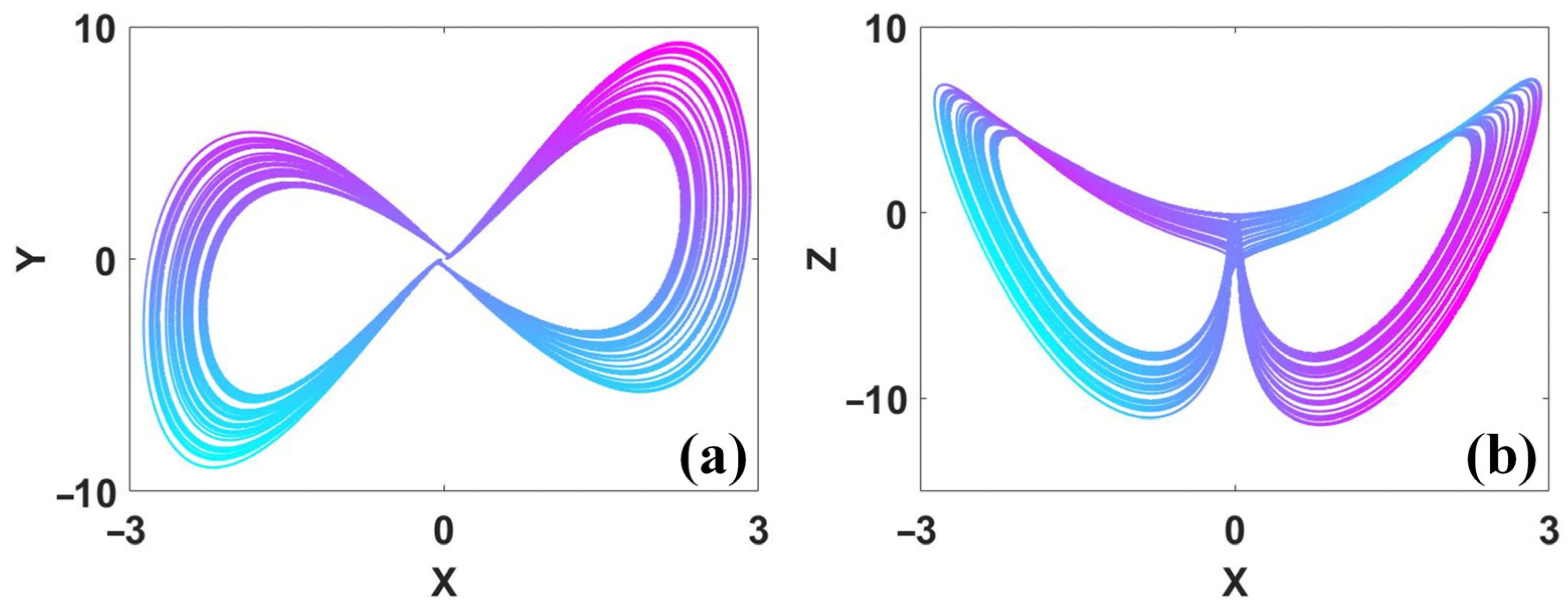
The topology of a symmetric system typically means that the structure of its solution is also symmetric. In a reflection-symmetric system, the coexisting pair of attractors have the single possibility of broken polarities. As an obviously typical system, the Lorenz system gives such an attractor of a symmetric structure. We know that the Lorenz system is one of rotational symmetry since the polarity reversals of x and y do not destroy the polarity balance [51].

$$\{\begin{array}{l}\dot{x}=\sigma (y-x),\\ \dot{y}=-xz+rx-y,\\ \dot{z}=xy-bz.\end{array}$$

(1)

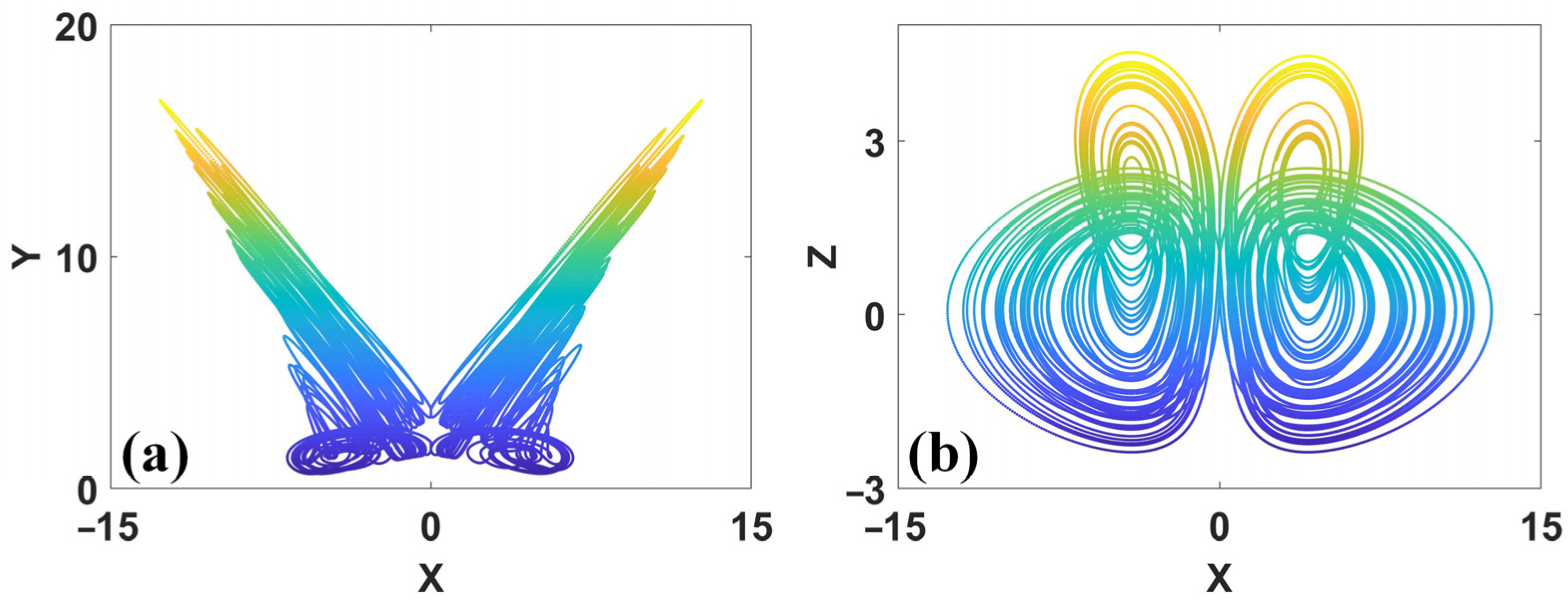
And thus, system (1) gives a rotational symmetric attractor as shown in Figure 2. The structure of the attractor shows a beautiful double-wing structure.

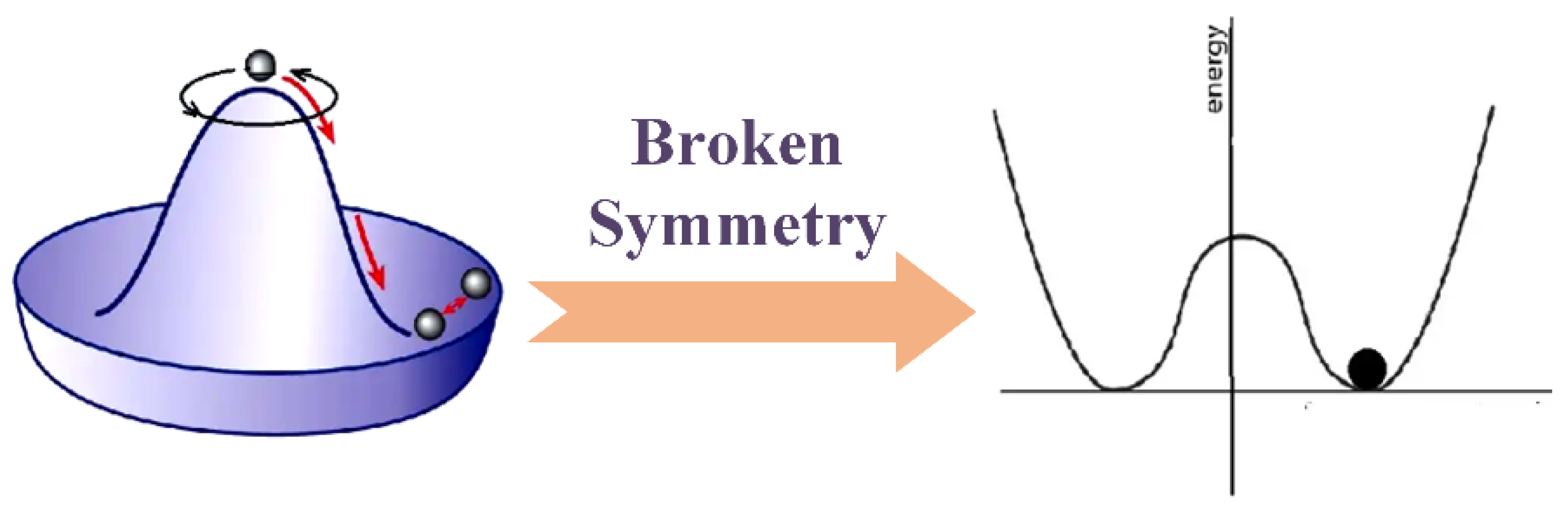
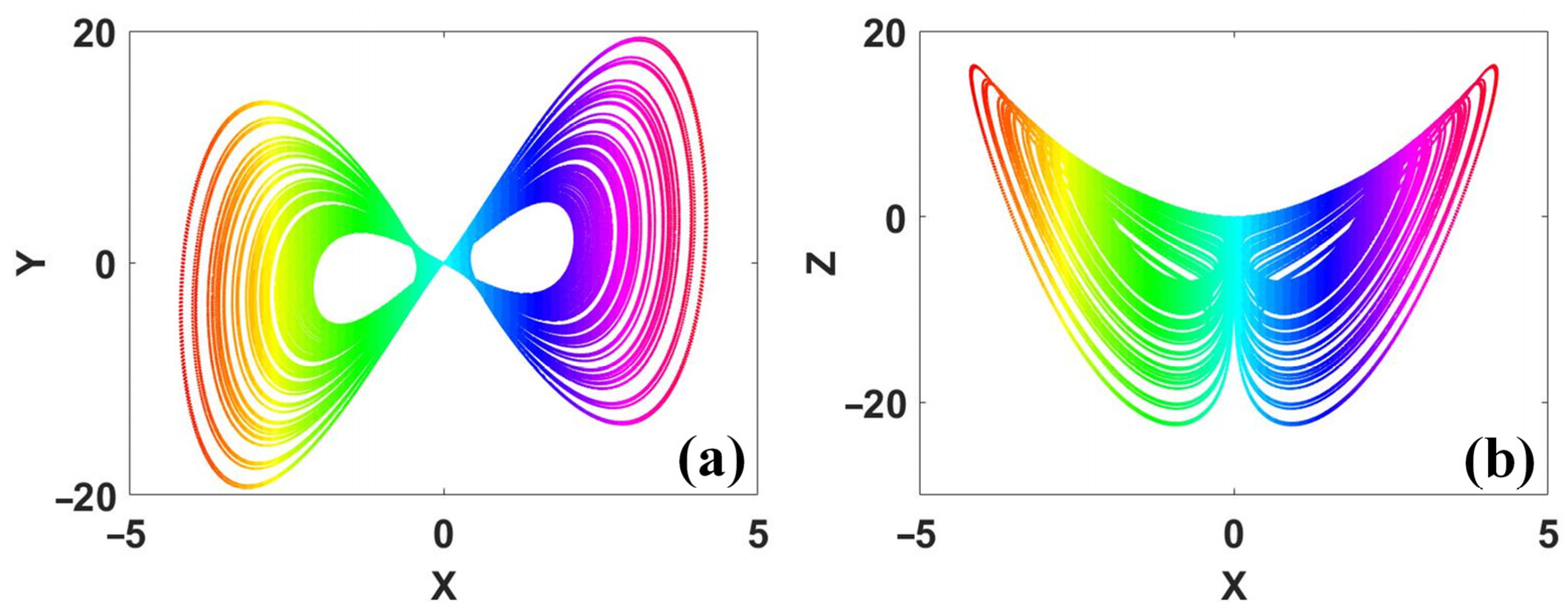
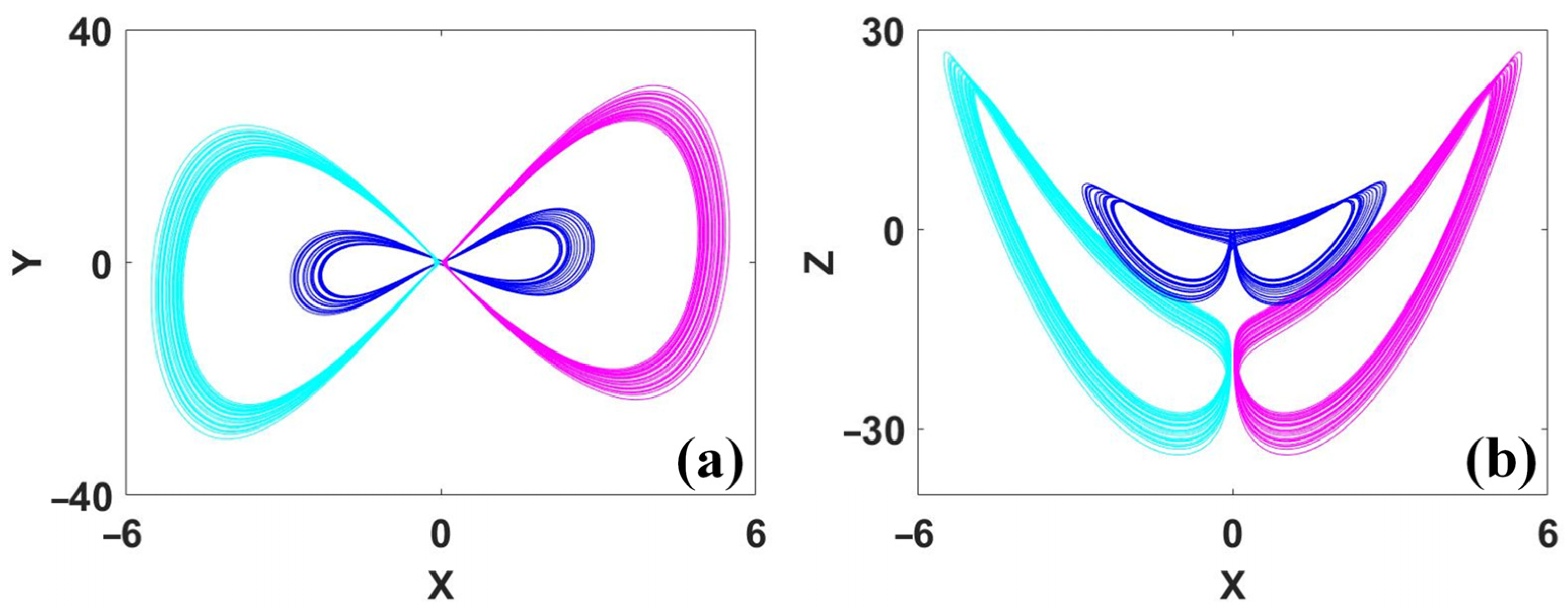
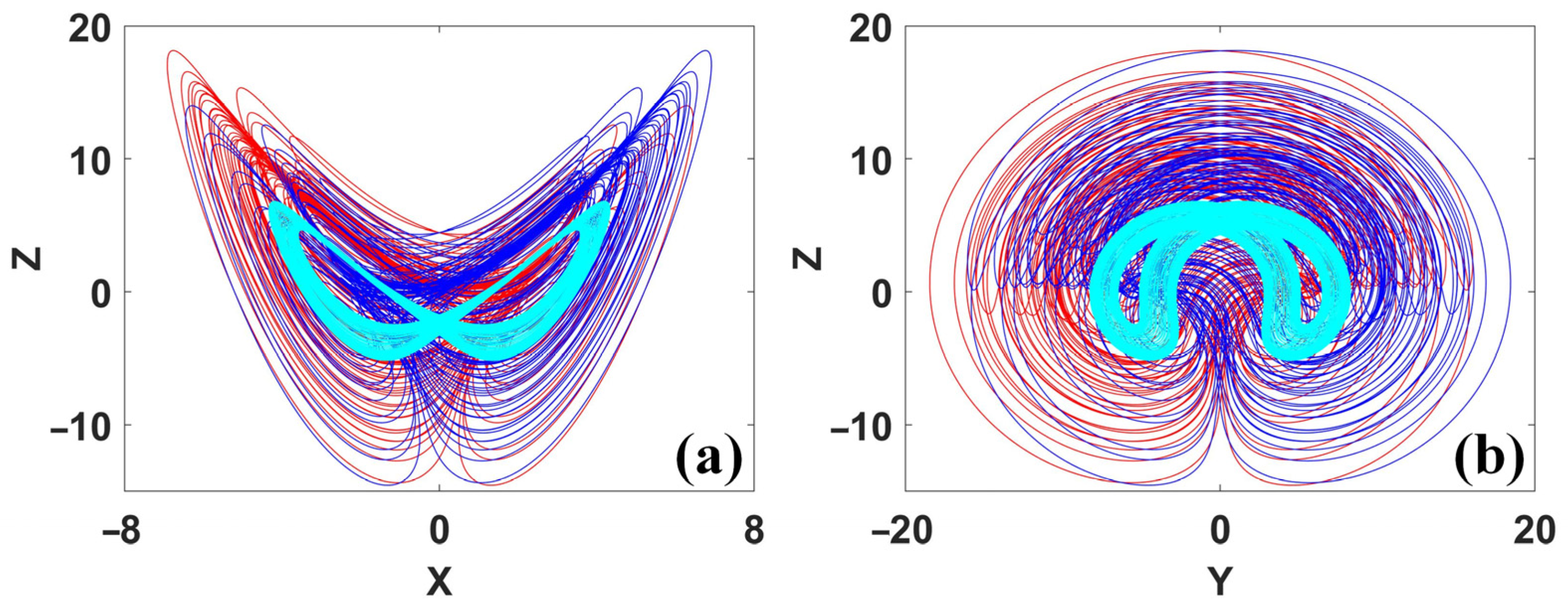
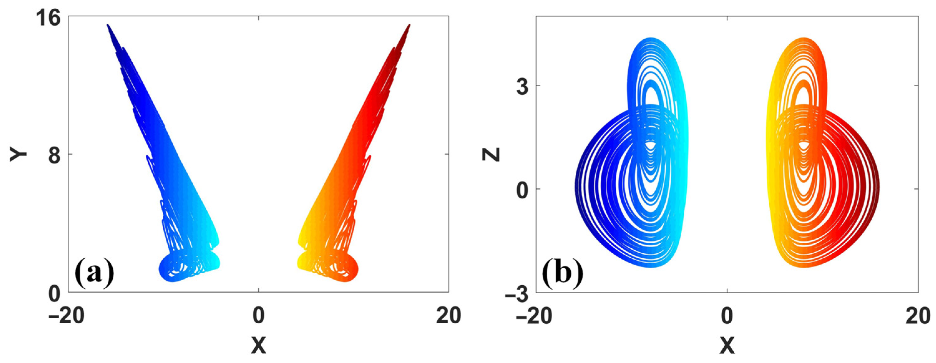
Broken symmetry will bring pairs of independent solutions for the local stability, as shown in Figure 3. In this case, different polarities represent those independent zones with separated solutions. As shown in Figure 4, when the parameters are σ = 0.256, r = 0, b = −0.3, a symmetric pair of coexisting attractors appears. Note that here, the coexisting attractors occupy the regions of x in the regions of positive and negative polarities separately, but for the dimension y, all attractors share the same bipolar space. In some specific circumstances, a symmetric attractor may coexist with pairs of asymmetric attractors. As shown in Figure 5, when σ = 0.279, r = 0, b = −0.3, three chaotic attractors coexist, one of which is a symmetric attractor with bipolar x and y, and the other two are the symmetric pair of attractors with positive x and negative x.

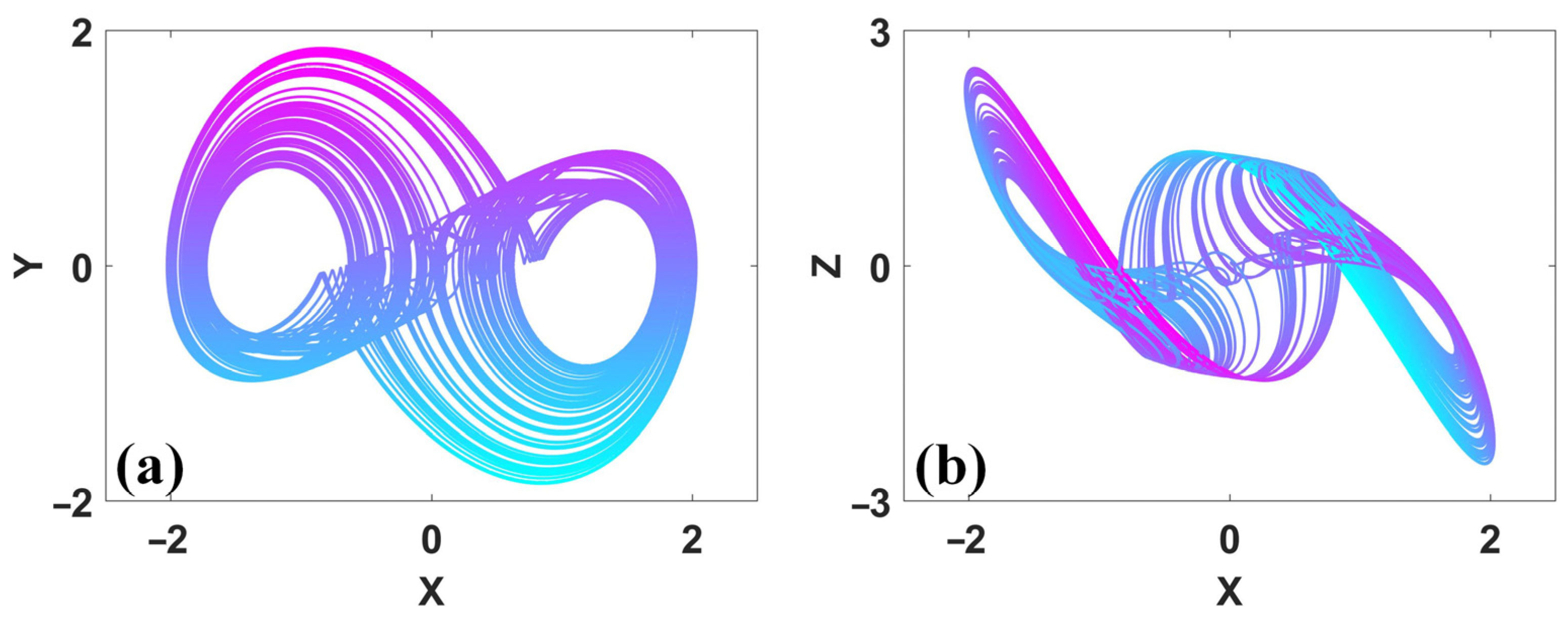
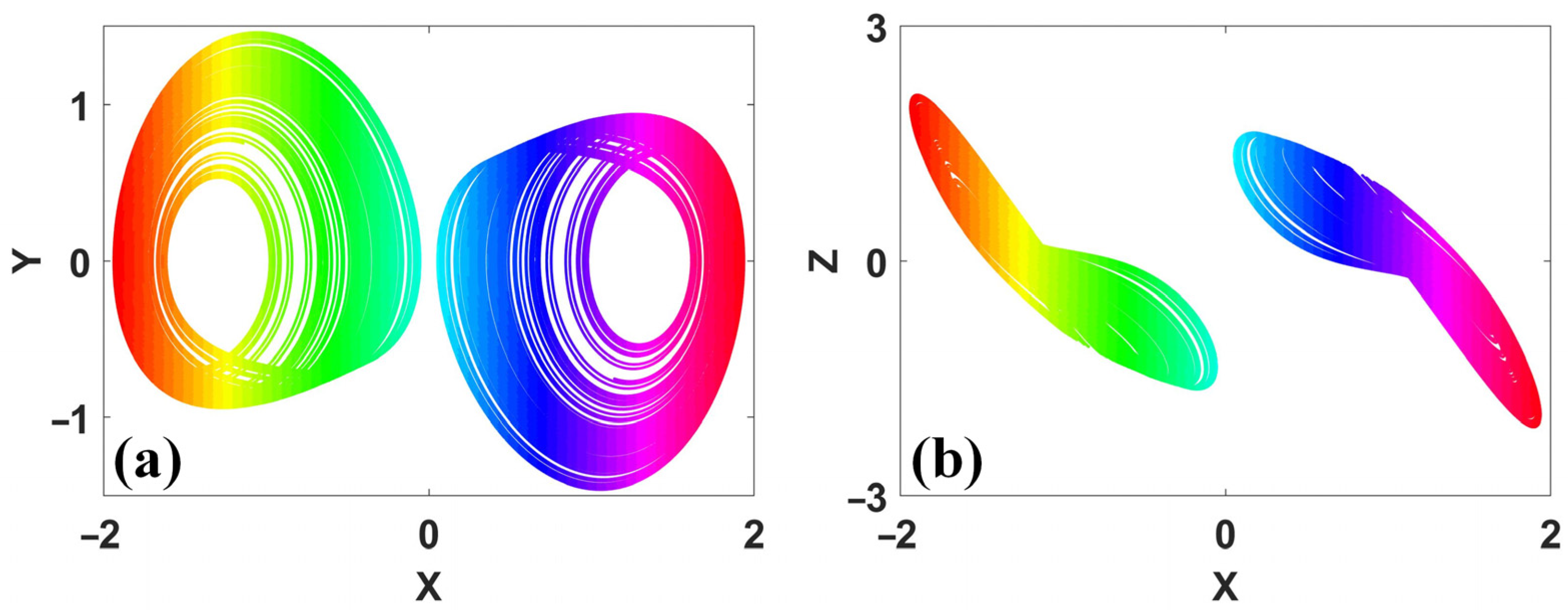
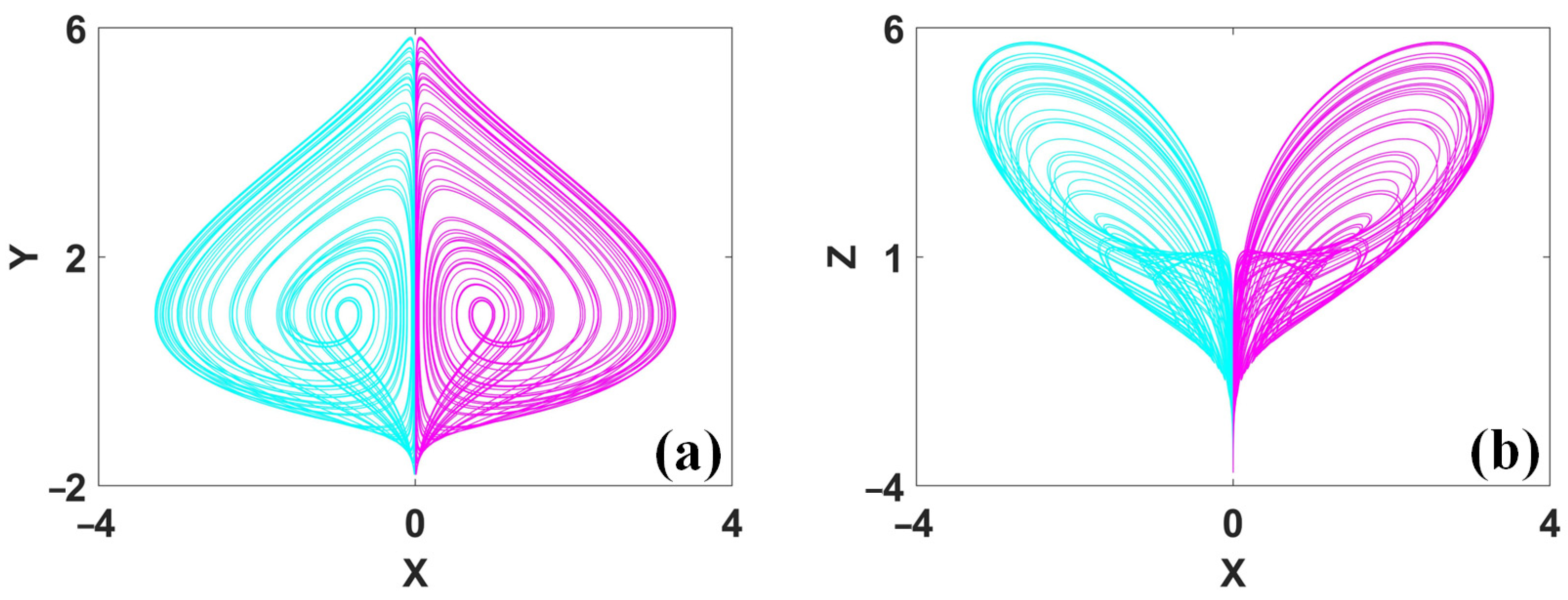
For other regimes of symmetric systems, the power of broken symmetry also leads to coexisting symmetric pairs of attractors. For a system of inversion symmetry, such as system (2) [51], the symmetric attractor crosses the zone of positive and negative polarities, shown in Figure 6. But for the case of broken symmetry, the coexisting pair of attractors has broken polarities of x; meanwhile, the dimensions of y and z share the whole polarity, as shown in Figure 7. For the system of reflection symmetry, the coexisting pair of attractors can only stand in separated phase spaces divided by the dimension with polarity reversal. Let us see the example of system (3) [51]: when the symmetry is broken, the symmetric attractor turns out to be two petals of coexisting attractors, as shown in Figure 8 and Figure 9.

$$\{\begin{array}{l}\dot{x}=y,\\ \dot{y}=z,\\ \dot{z}=-z-ay-x^3+bx.\end{array}$$

(2)

$$\{\begin{array}{l}\dot{x}=x-xy,\\ \dot{y}=z,\\ \dot{z}=-y-az+x^2.\end{array}$$

(3)

2.3. Diversities of Stability in Symmetric Systems

Symmetric systems bursting out symmetric pairs of attractors seems to be associated with the equilibrium points. We can see that the symmetric structure is often combined with the same type of symmetric equilibrium points. When symmetry is broken, the system typically has corresponding symmetric equilibria, as listed in

Table 1. Coexisting equilibria under broken symmetry and corresponding stabilities [51,52].

Equations	Parameters	Equilibria	Eigenvalues
$\left\{\begin{array}{l}\dot{x}=y \\ \dot{y}=z \\ \dot{z}=-z-ay-x^3+bx \end{array}\right.$ [51]	a = 2.1 b = 2	(0, 0, 0) ($\sqrt{2}$, 0, 0) ($-\sqrt{2}$, 0, 0)	(0.6366, $-$0.8183 $\pm$ 1.5723i) ($-$1.4516, 0.2258 $\pm$ 1.6446i)
$\left\{\begin{array}{l}\dot{x}=a(y-x) \\ \dot{y}=-xz+cx-y \\ \dot{z}=xy-bz \end{array}\right.$ [51]	a = 0.279 b = $-$0.3 c = 0	(0, 0, 0) ($\sqrt{30}/10$, $\sqrt{30}/10$, $-$1) ($-\sqrt{30}/10$, $-\sqrt{30}/10$, $-$1)	($-$1, $-$0.279, 0.3) ($-$1.1722, 0.0966 $\pm$ 0.3653i)
$\left\{\begin{array}{l}\dot{x}=y-x \\ \dot{y}=-xz \\ \dot{z}=xy-a \end{array}\right.$ [51]	a = 4.7	($\sqrt{470}/10$, $\sqrt{470}/10$, 0) ($-\sqrt{470}/10$, $-\sqrt{470}/10$, 0)	($-$1.6369, 0.3185 $\pm$ 2.3751i)
$\left\{\begin{array}{l}\dot{x}=y-bx \\ \dot{y}=yz-x \\ \dot{z}=a-y^2 \end{array}\right.$ [51]	a = 1 b = 1.06	(50/53, 1, 50/53) ($-$50/53, $-$1, 50/53)	($-$0.8218, 0.3526 $\pm$ 1.5669i)
$\left\{\begin{array}{l}\dot{x}=x-xy \\ \dot{y}=z \\ \dot{z}=-y-az+x^2\end{array}\right.$ [51]	a = 0.7	(0, 0, 0) (1, 1, 0) ($-$1, 1, 0)	(1, $-$0.35 $\mp$ 0.9368i) ($-$1.2216, 0.2608 $\pm$ 1.2527i)
$\left\{\begin{array}{l}\dot{x}=y-x \\ \dot{y}=-axz+u \\ \dot{z}=xy-1 \\ \dot{u}=-by \end{array}\right.$ [52]	a = 6 b = 0.1	None	None

. Symmetric systems typically have an equilibrium of the origin (0, 0, 0), which can be considered to satisfy any condition of symmetry. The eigenvalues of the equilibria could be various combinations, indicating they are saddle-foci, index-1 saddle points, or nonhyperbolic equilibrium points. Note that the symmetry type of the coexisting equilibria agrees with the topology of the system even when the symmetry is broken.

Sometimes, even when the chaotic system has no equilibrium point, the system still can exhibit symmetric pairs of coexisting attractors, in which case, all the attractors are named as hidden attractors [52]. One example is the simple seven-term system with two quadratic nonlinearities.

$$\{\begin{array}{l}\dot{x}=y-x,\\ \dot{y}=-xz+u,\\ \dot{z}=xy-a,\\ \dot{u}=-by.\end{array}$$

(4)

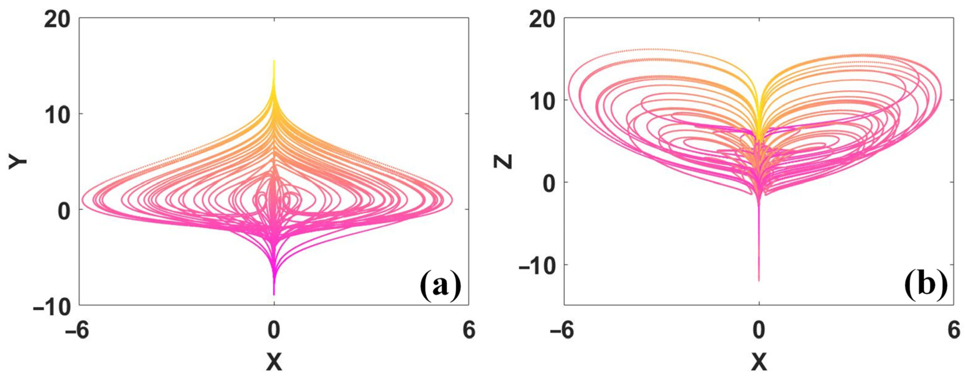
This is exactly the diffusionless Lorenz system with an added variable u. The coefficients of five of the seven terms can be normalized to ±1 through a linear rescaling of the four variables and time without loss of generality; system (1) is completely described by only two independent parameters, taken here as a and b. Although system (4) has no equilibrium point, system (4) can still give chaotic or even hyperchaotic solutions [53,54]. For example, when a = 6, b = 0.1, a quasi-periodic torus coexists with a symmetric pair of chaotic attractors, as shown in Figure 10.

3. Offset Boosting for Symmetric Pairs of Strange Attractors

Symmetry can also be reconstructed even though the system is an asymmetric one. In this way, the desired number of coexisting symmetric pairs of attractors can be obtained. And even the distances between the coexisting pairs of attractors can be defined. If a variable substitution ${u_i=x_i,u}_j=x_j+d_j$, (here, $1\le j\le N$,$i\in \left\{1,2,\dots ,N\right\}\backslash \left\{j\right\}$) in a dynamical system $\dot{X}=F\left(X\right)$ ($X=\left(x_1,x_2,\dots ,x_N\right))$ leads to $\dot{U}=F(U,d_j)$ ($U=\left(u_1,u_2,\dots ,u_N\right))$, the variable $x_j$ in system $\dot{X}=F\left(X\right)$ obtains the operation of offset boosting, and for this reason its average value is boosted by the new introduced constant $d_j$. The variable $x_j$ can be a signal in an electrical system, and correspondingly, the signal is offset-boosted by a direct current voltage of $d_j$. When the operation ${u_i=x_i,u}_j=x_j+d_j$ only introduces an independent constant $d_j$ in one dimension in the system, then the system is named a variable-boostable system [55]. For a variable-boostable dynamical system $\dot{X}=F\left(X\right)=\left(f_1\right(X),f_2(X),\dots ,f_N(X\left)\right)$ ($X=\left(x_1,x_2,\dots ,x_{i_0},\dots ,x_N\right))$, there exists one and only one $f_{j_0}(x_1,x_2,\dots ,x_{i_0},\dots ,x_N)$ ($i_0{\ne j}_0$) satisfying $f_{j_0}\left(x_1,x_2,\dots ,x_{i_0},\dots ,x_N\right)=h_{j_0}\left(x_1,x_2,\dots ,x_{i_0-1},x_{i_0+1},\dots ,x_N\right)+k{x}_{i_0}$, where k is a nonzero constant.

Offset boosting is an effective technique for shifting an attractor in phase space without changing the basic dynamics of a system [56,57,58,59,60,61,62]. In a system $\dot{X}=F\left(X\right)$, $X=\left(x_1,x_2,\dots ,x_n\right)$, take the substitution of ${u_i=x_i,u}_j=x_j+d_j$, $i\in \left\{1,2,\dots ,n\right\}\backslash \left\{j\right\}$, $1\le j\le N$, and the offset of the variable $x_j$ is boosted. The offset parameter $d_j$ controls the attractor to switch between the negative zone and the positive one according to the dimension of $x_j$, $1\le j\le N$. In fact, an attractor can be moved in any dimension by offset boosting. From this view, when the offset boosting is completed by an absolute-value function, corresponding attractors can be doubled by the combination of polarity compensation. The mechanism is as explained in [63,64,65].

For a dynamical system,

$$\{\begin{array}{l}{\dot{x}}_1=f_1(x_1,x_2,\cdots ,x_n),\\ {\dot{x}}_2=f_2(x_1,x_2,\cdots ,x_n),\\ \cdots \\ {\dot{x}}_n=f_n(x_1,x_2,\cdots ,x_n).\end{array}$$

(5)

If system (5) has coexisting solutions identified by attractors like, $O_1,O_2,\dots ,O_m$, take the offset-boosting constants as $d_s>0,s=1,2,\dots ,n$, subjecting to any state vector $\left(x_1,x_2,\dots ,x_m\right)\in O_1\cup O_2\cup \dots \cup O_m$ to satisfy ${|x}_1|<d_1,{|x}_2|<d_2,\dots ,{|x}_n|<d_n$, then substituting $x_i$ with ${|x}_i|-d_i$, $i\in \left\{1,2,\dots ,n\right\}$ into system (5) like,

$$\{\begin{array}{l}{\dot{x}}_1=f_1(x_1,x_2,\cdots ,x_{i-1},|x_i|-d_i,x_{i+1},\dots ,x_n),\\ {\dot{x}}_2=f_2(x_1,x_2,\cdots ,x_{i-1},|x_i|-d_i,x_{i+1},\dots ,x_n),\\ \cdots \\ {\dot{x}}_i=\mathrm{sgn}(x_i)f_i(x_1,x_2,\cdots ,x_{i-1},|x_i|-d_i,x_{i+1},\dots ,x_n),\\ \cdots \\ {\dot{x}}_n=f_n(x_1,x_2,\cdots ,x_{i-1},|x_i|-d_i,x_{i+1},\dots ,x_n).\end{array}$$

(6)

Then:

(I)

System (6) is one of symmetry according to the dimension of $x_i$;

(II)

System (6) has 2 m coexisting attractors $O_{11},O_{12},\cdots ,O_{1m},O_{21},O_{22},\cdots ,O_{2m}$;

(III)

All the attractors $O_{kj}, k=1,2, j=1,2,\dots ,m,$ in system (6) share the same structure with the ones in system (5), and all the equilibria in system (6) have the same stabilities with those of system (5).

Take the above method for constructing coexisting attractors in the Rössler system [66,67,68], which is described by

$$\{\begin{array}{l}\dot{x}=-y-z,\\ \dot{y}=x+ay,\\ \dot{z}=b+z(x-c).\end{array}$$

(7)

We know, when a = b = 0.2, c = 5.7, the system is chaotic with Lyapunov exponents (LEs) of (0.0714, 0, −5.3943) and a Kaplan-Yorke dimension of D_KY = 2.0132. Replace the variable z with an absolute function |z| − d,

$$\{\begin{array}{l}\dot{x}=-y-(|z|-d),\\ \dot{y}=x+ay,\\ \dot{z}=\mathrm{sgn}(z)(b+(\left|z\right|-d)(x-c)).\end{array}$$

(8)

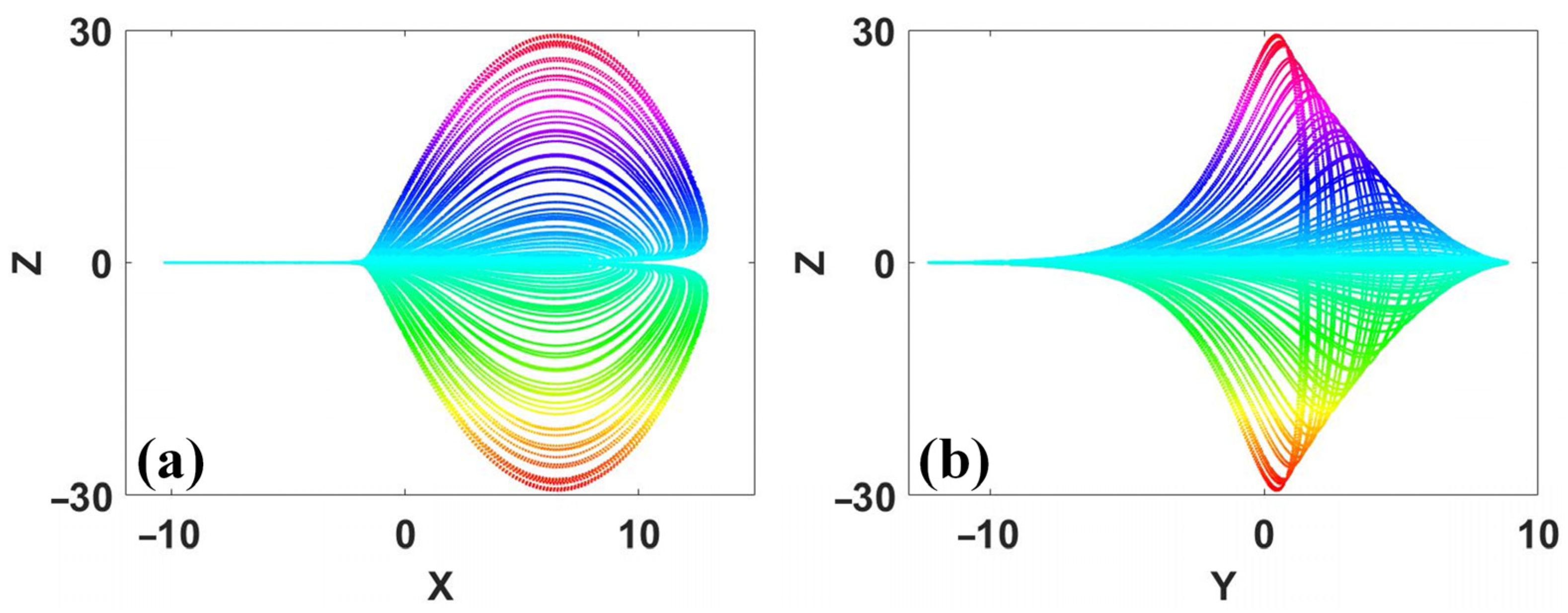
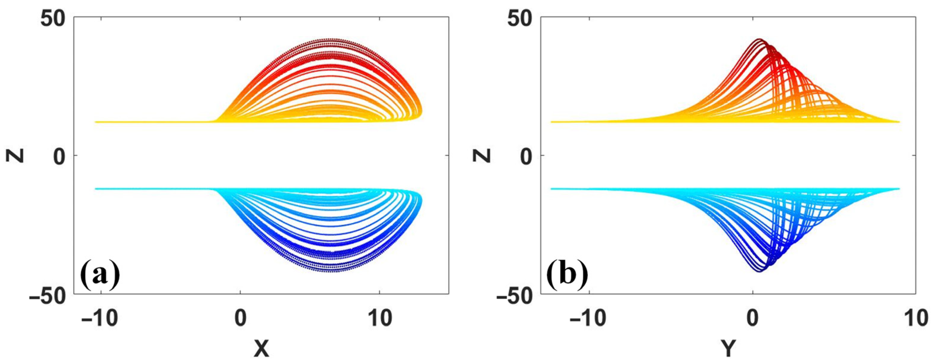
This time, system (8) turns out to be a reflection invariant system since it has polarity balance when z turns to be −z, and the attractors are doubled according to the z-axis, as shown in Figure 11. The larger offset constant d will separate the coexisting attractors farther away in this direction. For example, let d = 12, the two attractors stand in phase space far away, as shown in Figure 12. More absolute functions can turn the original Rössler system to be other regimes of symmetry. That is to say, take |x| − d₁, |y| − d₂, |z| − d₃, the derived system is one of inversion symmetry, and when the variables x, y, and z are polarity inversed, the derived system keeps the same equation, as written in system (9),

$$\{\begin{array}{l}\dot{x}=\mathrm{sgn}(x)(-(\left|y\right|-d_2)-(\left|z\right|-d_3)),\\ \dot{y}=\mathrm{sgn}(y)((\left|x\right|-d_1)+a(\left|y\right|-d_2)),\\ \dot{z}=\mathrm{sgn}(z)(b+(\left|z\right|-d_3)((|x|-d_1)-c)).\end{array}$$

(9)

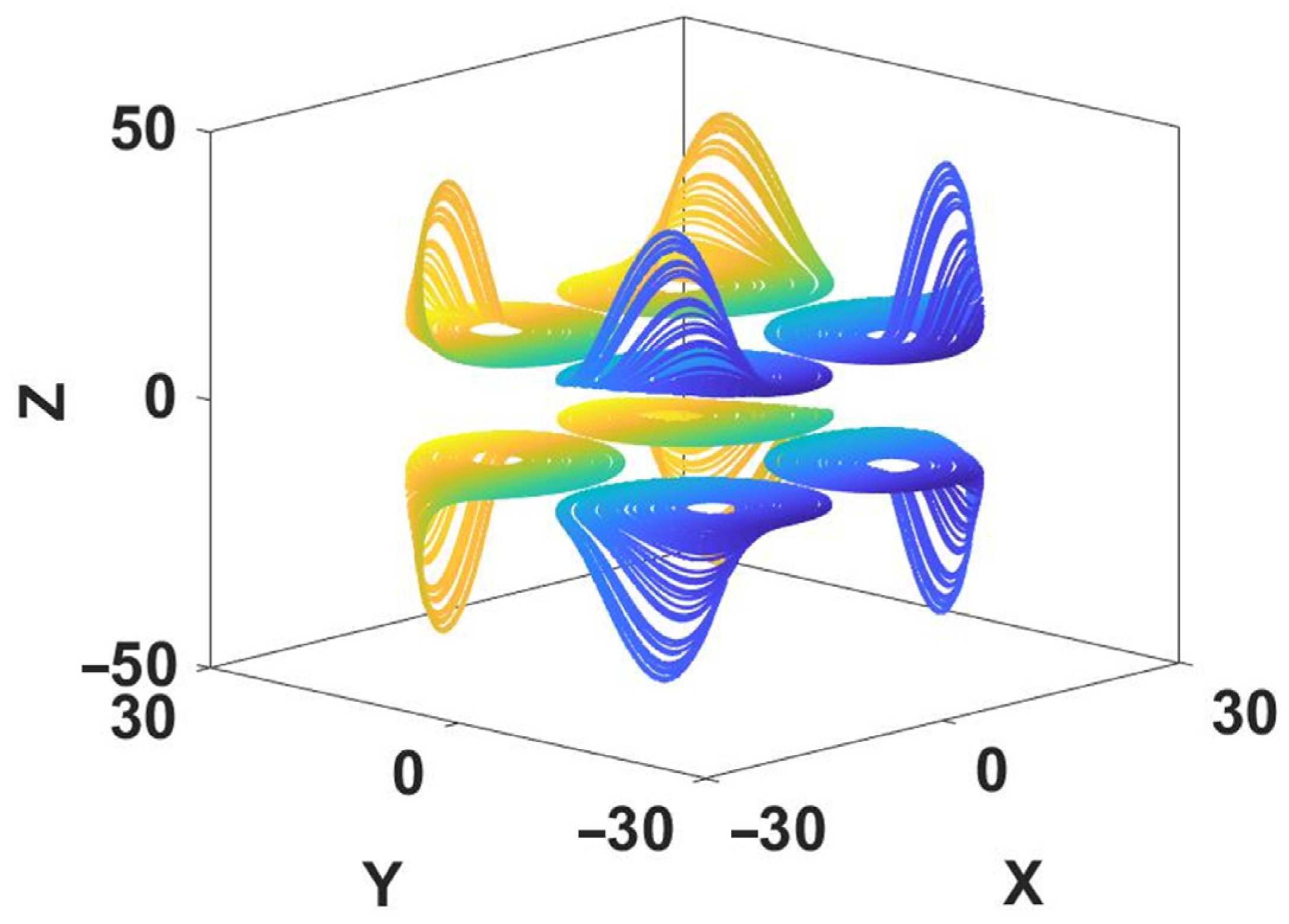
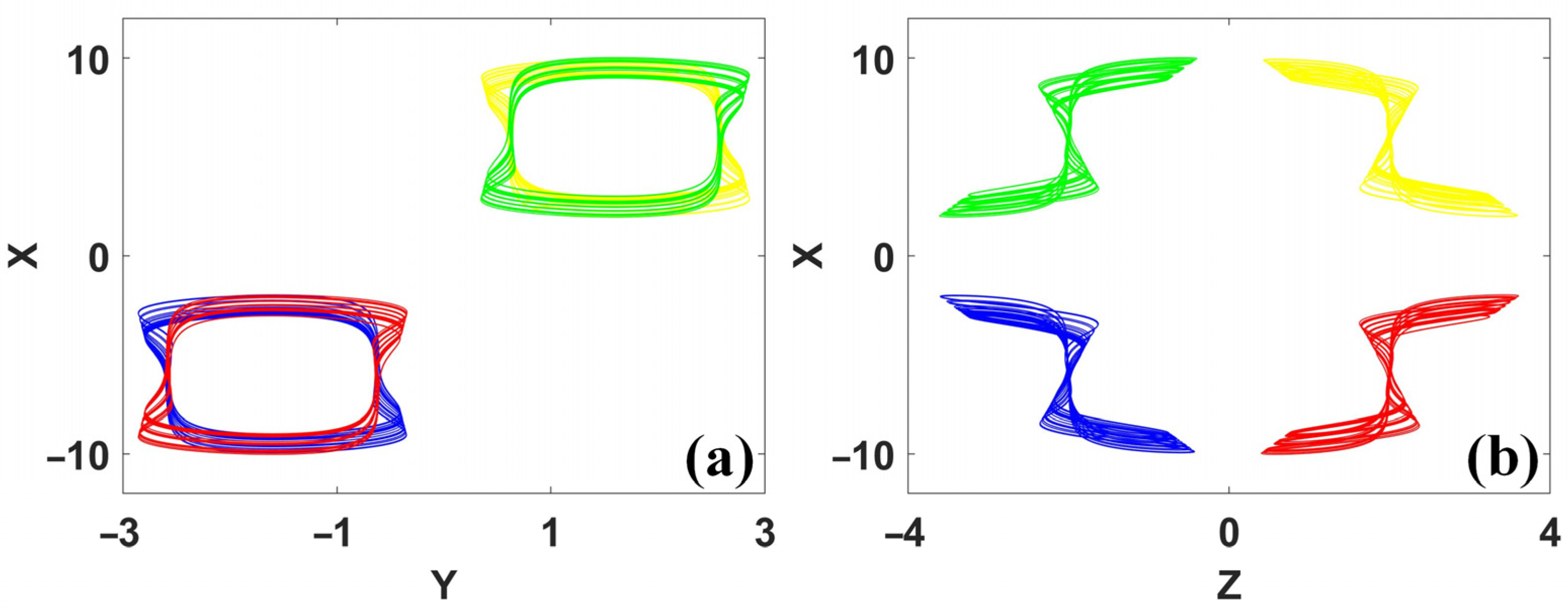
And at this time, the original attractor has three instances of doubling and in total eight attractors appear, as displayed in Figure 13.

4. Coexisting Strange Attractors of Conditional Symmetry

The polarity balance cannot always be preserved when the polarities of some of the variables are reversed. Sometimes an additional operation with some of the variables can return the polarity balance and lead to conditional symmetry. As we know, a system variable like x can be written as x = |x|sgn(x). In fact, any variable in an equation includes two types of inherent features: the amplitude and the polarity of the variable. Therefore, there are two effective polarity adapters: one is the signum function for maintaining the polarity, and the other is the absolute value function removing the polarity. The combination of the signum function and the absolute-value function can produce coexisting doubled attractors. At the same time, the absolute-value function is an effective way of producing functional polarity reversal leading to coexisting conditional symmetric attractors [69,70,71,72,73,74,75,76]. Therefore, from the conception of conditional symmetry, we could conclude that if some of the variables are the polarities reversed, the additional operation like offset boosting may return the polarity balance and result in symmetrical attractor doubling or conditional symmetry, as shown in Figure 14. The polarity adapter and slide polarity converter are widely applied in a dynamical system for giving conditional symmetry or for attractor self-reproduction.

For a dynamical system $\dot{X}=F\left(X\right)=\left(f_1\right(X),f_2(X),\dots ,f_N(X\left)\right)$ ($X=\left(x_1,x_2,\dots ,x_N\right))$, when the variable substitution including polarity reversal and offset boosting such as $u_{i_1}={-x}_{i_1},u_{i_2}={-x}_{i_2},\cdots ,u_{i_k}={-x}_{i_k},u_{j_1}=x_{j_1}+d_{j_1},u_{j_2}=x_{j_2}+d_{j_2},\cdots ,u_{j_l}=x_{j_l}+d_{j_l},u_i=x_i$, (here, $1\le i_1,\cdots ,i_k\le N$,$1\le j_1,\cdots ,j_l\le N$, $i_1,\cdots ,i_k$ and $j_1,\cdots ,j_l$ are not identical, $i\in \left\{1,2,\dots ,N\right\}\backslash \{i_1,\cdots ,i_{k,}{j}_1,\cdots ,j_{l,}\}$) leads to the derived system retaining its polarity balance and satisfies $\dot{U}=F\left(U\right)$ ($U=\left(u_1,u_2,\dots ,u_N\right)$, then the system $\dot{X}=F\left(X\right)$ ($X=\left(x_1,x_2,\dots ,x_N\right))$ is one of one-dimensional conditional symmetry since the polarity balance needs one-dimensional offset boosting. For a three-dimensional system, $\dot{X}=F\left(X\right)$ ($X=\left(x_1,x_2,x_3\right))$, the regime could be conditional rotational symmetry in one dimension or conditional reflection symmetry in one dimension or two dimensions.

The mechanism of conditional symmetry is associated with offset boosting for polarity balance. Suppose we want to construct a conditional reflection symmetric system. Here, the variable $x_i$ is polarity reversed, which will revise the polarity of ${\dot{x}}_i$ and in turn requires the polarity reversal on the right-hand side of ${\dot{x}}_i$ to obtain ${-f}_i\left(X\right)$ without influencing any of the other dimensions for polarity balance. To this end, based on exhaustive researching, a chaotic system of conditional reflection symmetry was found as shown,

$$\{\begin{array}{l}\dot{x}=y^2-0.4z^2,\\ \dot{y}=-z^2-1.75y+3,\\ \dot{z}=yz+(|x|-3).\end{array}$$

(10)

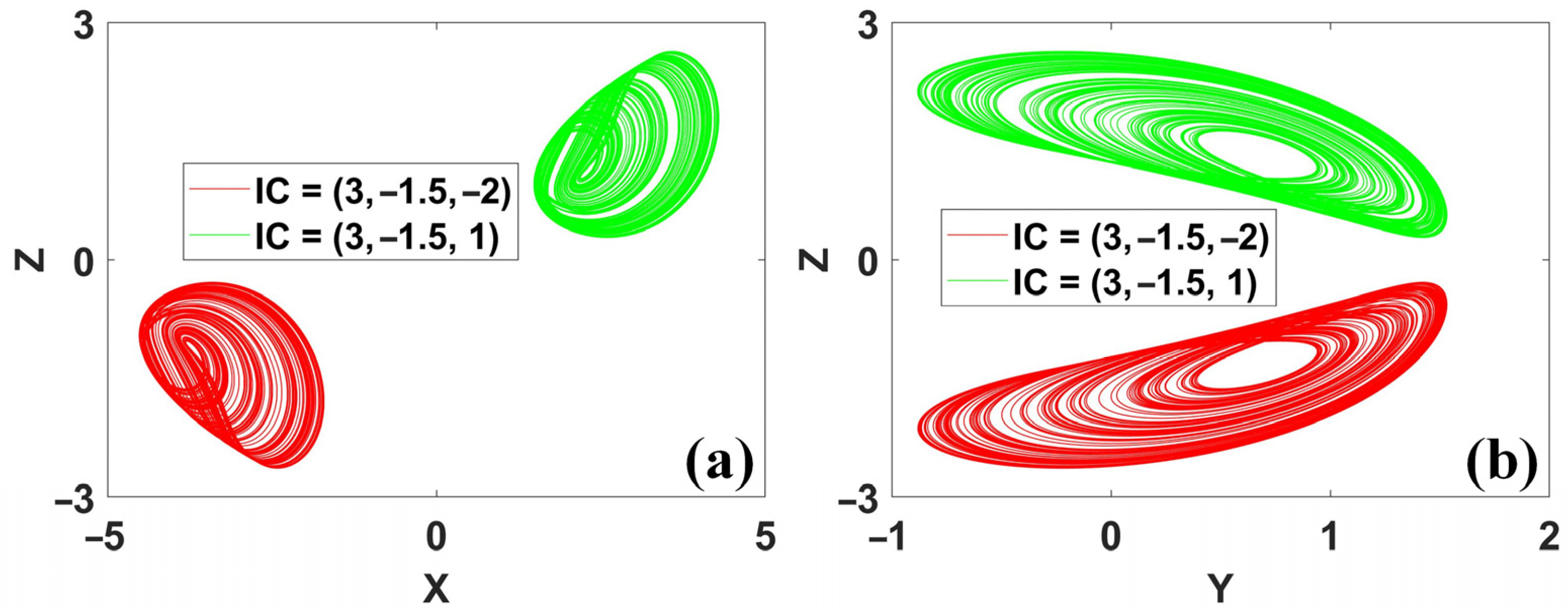
When z is polarity reversed, the polarity of the last dimension is destroyed unless the function F(x) = |x| − 3 obtains a reversed polarity to recover this balance. The polarity reversal of F(x) is induced by the offset boosting of x; that is to say, when x → x + d, the first two dimensions do not change, but the function F(x + d) turns out to be −F(x) since the absolute-value function has two reverse slopes during different positions of its variable. The newly balanced polarity brings a pair of coexisting attractors across the x- and z-axes in phase space, as shown in Figure 15. We see that the direction of the attractor in the dimension of x does not change, but the direction in the dimension of z is overturned. Therefore, we can call this polarity balance a ‘one-jump polarity balance’. Here, the polarity reversal of z depends on the offset boosting in the dimension of x. We call the operation of ‘offset boosting’ as ‘one jump’. This balance is therefore called ‘one-jump polarity balance’.

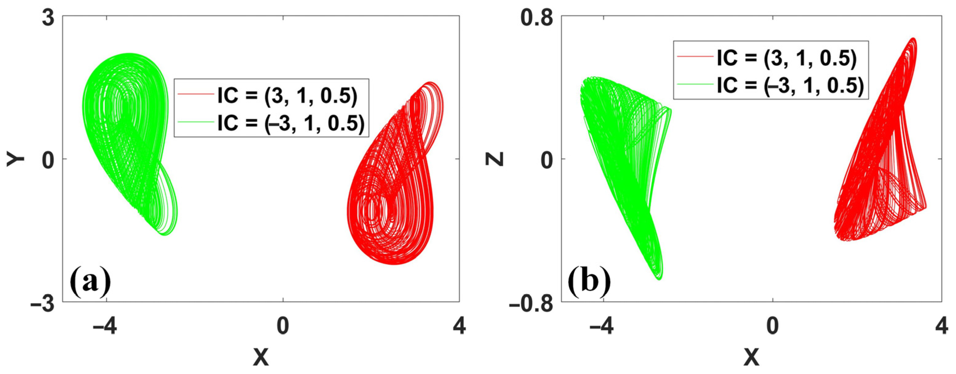
The ‘one-jump polarity balance’ can also happen in rotational symmetric systems. As for system (11), here, the polarity reversal in the dimensions y and z breaks the polarity balance in the last dimension until the offset boosting of x returns its balance without destroying the first dimension since adding a constant term does not change the value of the derivative. As shown in Figure 16, this time the direction of the coexisting attractors does not change in the x-axis but changes in both the y and z dimensions.

$$\{\begin{array}{l}\dot{x}=y^2-1.22,\\ \dot{y}=8.48z,\\ \dot{z}=-y-z+(|x|-3).\end{array}$$

(11)

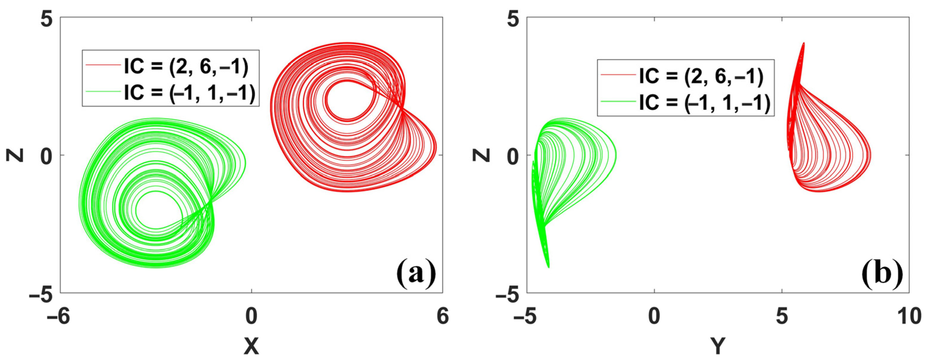
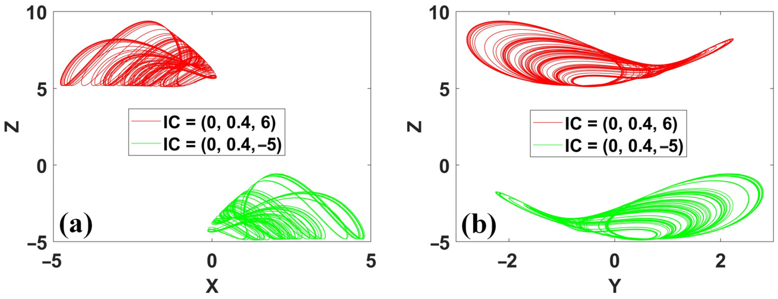
Sometimes, more operations of offset boosting are needed for balancing the polarity reversal of some of the variables. At this time, the conditional symmetry could be marked by ‘two-jump polarity balance’ or ‘more-jump polarity balance’. Like system (12), here, the polarity reversal of z is washed out by the offset boosting in the dimensions of x and y. This time, we can see that the direction of the coexisting attractors does not change in the x and y dimensions but turns down in the z-axis, as shown in Figure 17. The ‘two-jump polarity balance’ may also happen in the same dimension and leave more variables for polarity reversal, as displayed in system (13). Here, two variables are polarity reversed like x and y, but the polarity balance is returned by the offset boosting in the z dimension. As shown in Figure 18, when compared with system (12), system (13) has coexisting attractors with opposite directions in the dimensions of x and y but with the same direction in the z dimension.

$$\{\begin{array}{l}\dot{x}=1-(|y|-5)z,\\ \dot{y}=a{z}^2-(|y|-5)z,\\ \dot{z}=\left|x\right|-3.\end{array}$$

(12)

$$\{\begin{array}{l}\dot{x}=-y,\\ \dot{y}=x+\left|z\right|-5,\\ \dot{z}=2y^2-x(|z|-5)-a.\end{array}$$

(13)

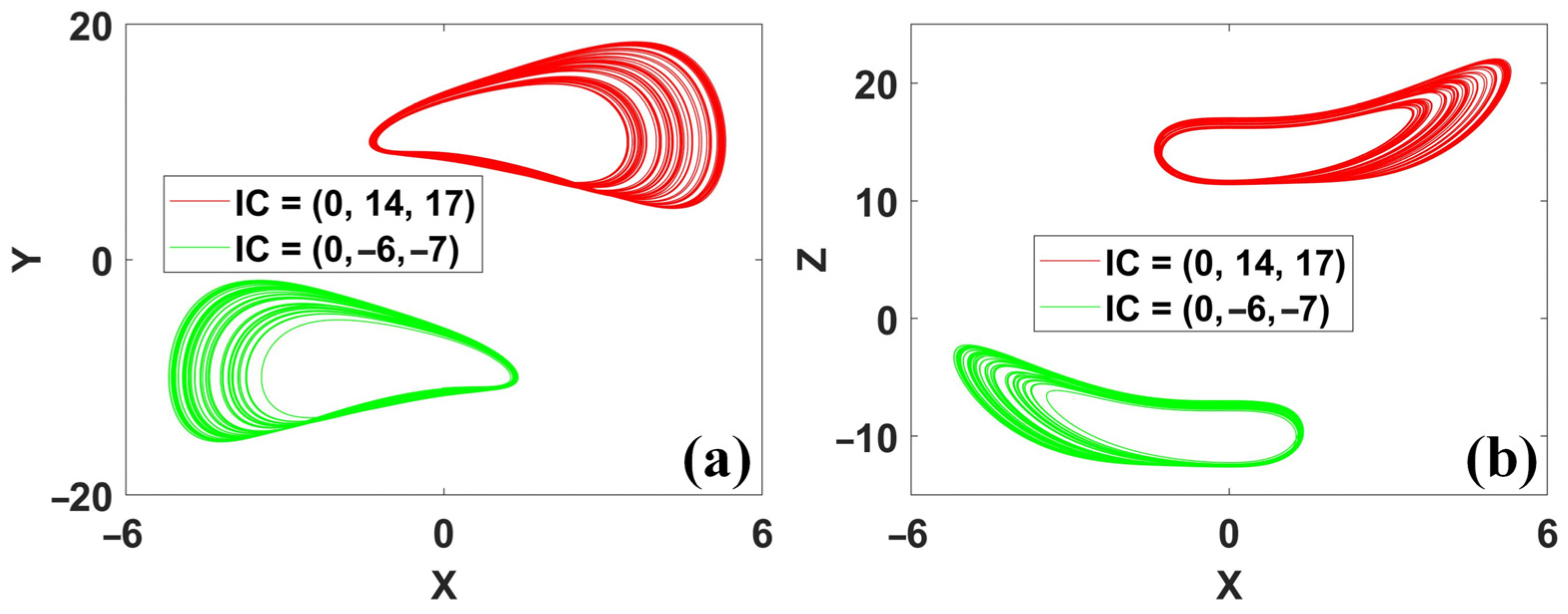
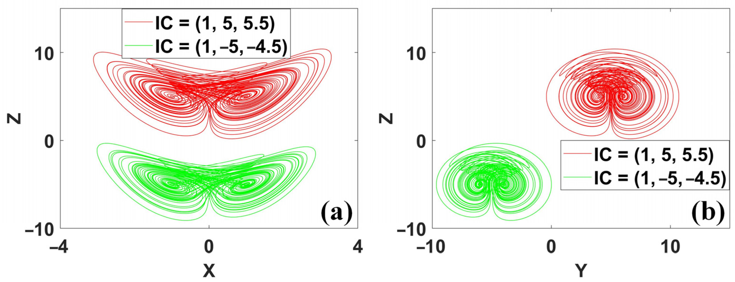
More operations of offset boosting from the absolute-value functions could be introduced for recovering the polarity balance, such as in system (14), which contains six absolute-value functions for balancing the polarity reversal of the variable x. As shown in Figure 19, here, the direction of the coexisting attractors in the x dimension is reversed, but the direction does not change in the y and z dimensions except for the two-dimensional offset boosting. More interestingly, sometimes conditional symmetry may happen in symmetric systems. In this case, the offset boosting of some of the system variables also may return other types of conditional symmetry. As we know, the original version of system (15) is the simplified Lorenz system, but the two-dimensional offset boosting with y and z returns a conditional reflection symmetry, as shown in Figure 20. Note that system (5) is an asymmetric system now, although it has symmetric attractors in a conditionally symmetric way, which means an asymmetric system may host symmetric attractors.

$$\{\begin{array}{l}\dot{x}=\left|y\right|-10,\\ \dot{y}=a(|y|-10)(|y|-10)-x(|z|-12),\\ \dot{z}=x^2+x(|y|-10)-bx(|z|-12).\end{array}$$

(14)

$$\{\begin{array}{l}\dot{x}=\left|y\right|-5-x,\\ \dot{y}=-x(|z|-5),\\ \dot{z}=x(|y|-5)-1.\end{array}$$

(15)

Many candidates of chaotic systems with coexisting attractors have been explored based on various system structures, such as those of chaotic systems with hidden attractors [70]. More candidates of chaotic systems with conditional symmetry [69,70,71,72,73,74,75] are listed in

Table 2. Chaotic systems of conditional symmetry proposed in [69,70,71,72,73,74,75].

Equations	Parameters	(x0, y0, z0)	LEs	DKY
$\left\{\begin{array}{l}\dot{x}=y^2-a{z}^2 \\ \dot{y}=-z^2-by+c \\ \dot{z}=yz+\mathrm{F}\left(x\right) \end{array}\right.$ [69] F(x) = |x| $-$ 3	a = 0.4 b = 1.75 c = 3	(3, $-$1.5, $-$2) (3, $-$1.5, 1)	0.1191, 0, $-$1.2500	2.0953
$\left\{\begin{array}{l}\dot{x}=y^2-a \\ \dot{y}=bz \\ \dot{z}=-y-z+\mathrm{F}\left(x\right) \end{array}\right.$ [69] F(x) = |x| $-$ 3	a = 1.22 b = 8.48	(3, 1, 0.5) ($-$3, 1, 0.5)	0.2335, 0, $-$1.2335	2.1893
$\left\{\begin{array}{l}\dot{x}=\mathrm{F}\left(y\right) \\ \dot{y}=z \\ \dot{z}=-x^2-az+b{\left(\mathrm{F}\right(y\left)\right)}^2+1\end{array}\right.$ [69] F(y) = |y| $-$ 4	a = 2.6 b = 2	(0.5, 4, $-$1) (0.5, $-$4, $-$1)	0.0463, 0, $-$2.6463	2.0175
$\left\{\begin{array}{l}\dot{x}=y \\ \dot{y}=\mathrm{F}\left(z\right) \\ \dot{z}=x^2-a{y}^2+bxy+x\mathrm{F}\left(z\right) \end{array}\right.$ [69] F(z) = |z| $-$ 8	a = 1.24 b = 1	(4, 0.8, $-$2) (4, 0.8, 14)	0.0645, 0, $-$1.2582	2.0513
$\left\{\begin{array}{l}\dot{x}=1-\mathrm{G}\left(y\right)z \\ \dot{y}=a{z}^2-\mathrm{G}\left(y\right)z \\ \dot{z}=\mathrm{F}\left(x\right) \end{array}\right.$ [69] F(x) = |x| $-$ 3 G(y) = |y| $-$ 5	a = 0.22	($-$1, 1, $-$1) (2, 6, $-$1)	0.0729, 0, $-$1.6732	2.0436
$\left\{\begin{array}{l}\dot{x}=\mathrm{F}\left(y\right) \\ \dot{y}=\mathrm{G}\left(z\right)x \\ \dot{z}=-ax\mathrm{F}\left(y\right)-bx\mathrm{G}\left(z\right)-x^2+({\mathrm{F}\left(y\right))}^2 \end{array}\right.$ [69] F(y) = |y| $-$ 5 G(z) = |z| $-$ 5	a = 3 b = 1.2	(0, $-$6, $-$6) (0, 6, 6)	0.0506, 0, $-$0.2904	2.1735
$\left\{\begin{array}{l}\dot{x}=-y \\ \dot{y}=x+\mathrm{F}\left(z\right) \\ \dot{z}=2y^2+x\mathrm{F}\left(z\right)-a \end{array}\right.$ [70] F(z) = |z| $-$ 5	a = 0.35	(0, 0.4, 6) (0, 0.4, $-$5)	0.0776, 0, $-$1.5008	2.0517
$\left\{\begin{array}{l}\dot{x}=y \\ \dot{y}=-x+\mathrm{F}\left(z\right) \\ \dot{z}=-0.8z^2+{\mathrm{F}\left(z\right)}^2+a \end{array}\right.$ [70] F(z) = |z| $-$ 12	a = 2.0	(0, 2.3, 12) (0, $-$2.3, $-$12)	0.0252, 0, $-$6.8521	2.0037
$\left\{\begin{array}{l}\dot{x}=\mathrm{F}\left(z\right) \\ \dot{y}=x-y \\ \dot{z}=-4x^2+8xy+y\mathrm{F}\left(z\right)+a \end{array}\right.$ [70] F(z) = |z| $-$ 12	a = 0.1	(0.5, 0, 11) (0.5, 0, $-$13)	0.0665, 0, $-$2.0410	2.0326
$\left\{\begin{array}{l}\dot{x}=-y \\ \dot{y}=x+\mathrm{F}\left(z\right) \\ \dot{z}=xy+x\mathrm{F}\left(z\right)+0.2y\mathrm{F}\left(z\right)-a \end{array}\right.$ [70] F(z) = |z| $-$ 15	a = 0.4	(2.5, 0, 15) ($-$2.5, 0, $-$15)	0.1026, 0, $-$2.1275	2.0482
$\left\{\begin{array}{l}\dot{x}=y \\ \dot{y}=\mathrm{F}\left(z\right) \\ \dot{z}=x^2-y^2+ax\mathrm{F}\left(z\right)+y\mathrm{F}\left(z\right)\end{array}\right.$ [70] F(z) = |z| $-$ 15	a = 2.0	(1, 0, 11) (1, 0, $-$19)	0.0538, 0, $-$11.8591	2.0045
$\left\{\begin{array}{l}\dot{x}=y \\ \dot{y}=\mathrm{F}\left(z\right) \\ \dot{z}=x^2-y^2+xy+0.4x\mathrm{F}\left(z\right)+a\end{array}\right.$ [70] F(z) = |z| $-$ 30	a = 1.0	(0, 1, 26.1) (0, 1, $-$32.9)	0.1105, 0, $-$1.3882	2.0796
$\left\{\begin{array}{l}\dot{x}=z \\ \dot{y}=-ay-z\mathrm{F}\left(x\right) \\ \dot{z}=z-b{z}^2+y\mathrm{F}\left(x\right) \end{array}\right.$ [70] F(x) = |x| $-$ 9	a = 1.62 b = 0.2	(9, 1, 0.8) ($-$9, 1, 0.8)	0.0645, 0, $-$0.6845	2.0943
$\left\{\begin{array}{l}\dot{x}=\mathrm{G}\left(y\right) \\ \dot{y}=a{\mathrm{G}\left(y\right)}^2-x\mathrm{F}\left(z\right) \\ \dot{z}=x^2+x\mathrm{G}\left(y\right)-bx\mathrm{F}\left(z\right) \end{array}\right.$ [70] G(y) = |y| $-$ 10 F(z) = |z| $-$ 12	a = 0.4 b = 1	(0, 14, 17) (0, $-$6, $-$7)	0.0749, 0, $-$0.7390	2.1013
$\left\{\begin{array}{l}\dot{x}=y \\ \dot{y}=c\left|y\right|\mathrm{F}\left(z\right)+0.1y\left|y\right|-x \\ \dot{z}=0.5x^2-axy-bx\mathrm{F}\left(z\right) \end{array}\right.$ [70] F(z) = |z| $-$ 4	a = 0.8 b = 0.5 c = 0.5	(1, 0.5, 5) ($-$1, $-$0.5, $-$4)	0.0177, 0, $-$0.4092	2.0433
$\left\{\begin{array}{l}\dot{x}=ay-ax+e\mathrm{F}\left(z\right) \\ \dot{y}=cx-y-x\left|\mathrm{F}\right(z\left)\right|+u \\ \dot{z}=xy-b\left|\mathrm{F}\right(z\left)\right| \\ \dot{u}=-kx \end{array}\right.$ [71] F(z) = |z| $-$ 50	a = 10 b = 8/3 c = 28 k = 4 e = 2	(0, $-$0.3, 2, 0) (0, $-$0.3, 50, 0)	0.2563, 0.1674, 0, $-$14.0917	3.0301
$\left\{\begin{array}{l}\dot{x}=1-ayz \\ \dot{y}=z\left|z\right|-z \\ \dot{z}=F\left(x\right)-bz \end{array}\right.$ [72] F(x) = |x| $-$ 3	a = 3.55 b = 0.6	($-$3, 0, $-$1) (3, 0, $-$1)	0.1455, 0, $-$0.7455	2.1952
$\left\{\begin{array}{l}\dot{x}=y^2-a{z}^2 \\ \dot{y}=-z^2-by+c \\ \dot{z}=yz+\mathrm{F}\left(x\right) \end{array}\right.$ [73] F(x) = |x| $-$ 3	a = 0.4 b = 1.75 c = 3	(3, $-$1.5, $-$2) (3, $-$1.5, 1)	0.1191, 0, $-$1.2500	2.0953
$\left\{\begin{array}{l}\dot{x}=y^2-a \\ \dot{y}=bz \\ \dot{z}=-y-z+\mathrm{F}\left(x\right) \end{array}\right.$ [73] F(x) = |x| $-$ 3	a = 1.22 b = 8.48	(3, 1, 0.5) ($-$3, 1, 0.5)	0.2335, 0, $-$1.2335	2.1893
$\left\{\begin{array}{l}\dot{x}=\mathrm{F}\left(y\right) \\ \dot{y}=z \\ \dot{z}=-x^2-az+b{\left(\mathrm{F}\right(y\left)\right)}^2+1 \end{array}\right.$ [74] F(y) = |y| $-$ 4	a = 2.6 b = 2	(0.5, 4, $-$1) (0.5, $-$4, $-$1)	0.0463, 0, $-$2.6463	2.0175
$\left\{\begin{array}{l}\dot{x}=y \\ \dot{y}=\mathrm{F}\left(z\right) \\ \dot{z}=x^2-a{y}^2+bxy+x\mathrm{F}\left(z\right) \end{array}\right.$ [74] F(z) = |z| $-$ 8	a = 1.24 b = 1	(4, 0.8, $-$2) ($-$4, 0.8, 2)	0.0645, 0, $-$1.2582	2.0513
$\left\{\begin{array}{l}\dot{x}=1-\mathrm{G}\left(y\right)z \\ \dot{y}=a{z}^2-\mathrm{G}\left(y\right)z \\ \dot{z}=\mathrm{F}\left(x\right) \end{array}\right.$ [74] F(x) = |x| $-$ 3 G(y) = |y| $-$ 5	a = 0.22	($-$1, 1, $-$1) (2, 6, $-$1)	0.0729, 0, $-$1.6731	2.0436
$\left\{\begin{array}{l}\dot{x}=\mathrm{F}\left(y\right) \\ \dot{y}=x\mathrm{G}\left(z\right) \\ \dot{z}=-ax\mathrm{F}\left(y\right)-bx\mathrm{G}\left(z\right)-x^2+{\left(\mathrm{F}\right(y\left)\right)}^2 \end{array}\right.$ [74] F(y) = |y| $-$ 5 G(z) = |z| $-$ 5	a = 3 b = 1.2	(0, $-$6, $-$6) (0, 6, 6)	0.0506, 0, $-$0.2904	2.1742
$\left\{\begin{array}{l}\dot{x}=\mathrm{F}\left(y\right)-x \\ \dot{y}=-x\mathrm{G}\left(z\right) \\ \dot{z}=x\mathrm{F}\left(y\right)-a \end{array}\right.$ [75] F(y) = |y| $-$ 5 G(z) = |z| $-$ 5	a = 1	(1, 5, 6) (1, $-$5, $-$4)	0.2102, 0, $-$1.2102	2.1737
$\left\{\begin{array}{l}\dot{x}=ay\mathrm{G}\left(z\right) \\ \dot{y}=\mathrm{F}\left(x\right)-y \\ \dot{z}=1-y\mathrm{F}\left(x\right) \end{array}\right.$ [75] F(x) = |x| $-$ 7 G(z) = |z| $-$ 7	a = 1	(8, 1, 6) ($-$6, 1, $-$8)	0.2100, 0, $-$1.210	2.1736
$\left\{\begin{array}{l}\dot{x}=-\mathrm{G}\left(y\right)z \\ \dot{y}={\left(\mathrm{F}\right(x\left)\right)}^2-1 \\ \dot{z}=\mathrm{F}\left(x\right)-az \end{array}\right.$ [75] F(x) = |x| $-$ 4 G(y) = |y| $-$ 5	a = 2	(5, 6, $-$1) ($-$3, $-$4, $-$1)	0.0568, 0, $-$2.0568	2.0276
$\left\{\begin{array}{l}\dot{x}=az \\ \dot{y}=-x^2+1 \\ \dot{z}=bx-z-x\left|\mathrm{F}\right(y\left)\right| \end{array}\right.$ [75] F(y) = |y| $-$ 22	a = 18 b = 1.93	(1, 23, $-$1) ($-$1, $-$21, 1)	0.120, 0, $-$1.12	2.1071
$\left\{\begin{array}{l}\dot{x}=-ax+bx\left|\mathrm{F}\right(y\left)\right| \\ \dot{y}=-x^2+{\left(\mathrm{G}\right(z\left)\right)}^2+\mathrm{F}\left(y\right)\mathrm{G}\left(z\right) \\ \dot{z}=-c{\left(\mathrm{F}\right(y\left)\right)}^2-d\mathrm{F}\left(y\right)\mathrm{G}\left(z\right)+1 \end{array}\right.$ [75] F(y) = |y| $-$ 5 G(z) = |z| $-$ 12	a = 0.33 b = 0.75 c = 0.35 d = 0.9	(2, 1, $-$1) ($-$2, 1, $-$1)	0.0301, 0, $-$2.0419	2.0148
$\left\{\begin{array}{l}\dot{x}=-ax\left|\mathrm{F}\right(y\left)\right|+bx\left|z\right| \\ \dot{y}=-x^2-\mathrm{F}\left(y\right)z+1 \\ \dot{z}=c\mathrm{F}\left(y\right)+z \end{array}\right.$ [75] F(y) = |y| $-$ 3	a = 16.8 b = 2.8 c = 8.25	($-$1, 1, $-$1) (1, 1, $-$1)	0.2985, 0, $-$1.1319	2.2638
$\left\{\begin{array}{l}\dot{x}=-a\mathrm{F}\left(y\right)z+bx\left|\mathrm{F}\right(y\left)\right|-cx\left|z\right| \\ \dot{y}=x^2-z^2+d \\ \dot{z}=z+xF\left(y\right)-z\left|\mathrm{F}\right(y\left)\right| \end{array}\right.$ [75] F(y) = |y| $-$ 3	a = 7.3 b = 6.4 c = 118 d = 0.1	(1, 4, 1) ($-$1, $-$2, 1)	0.0708, 0, $-$25.6071	2.0028
$\left\{\begin{array}{l}\dot{x}=y-y\left|z\right| \\ \dot{y}=-y+y\left|\mathrm{F}\right(x\left)\right| \\ \dot{z}=a\mathrm{F}\left(x\right)\left|y\right|-bz\left|\mathrm{F}\right(x\left)\right| \end{array}\right.$ [75] F(x) = |x| $-$ 4	a = 1 b = 20	(5, 1, 3) ($-$3, 1, $-$3)	0.4543, 0, $-$20.4543	2.0222

, where the system equations, parameters, initial conditions, Lyapunov exponents (Les) and the corresponding Kaplan–York dimension (D_KY) are included. Those systems could be systems of symmetry or asymmetry or jerk systems. Readers could check these systems to see if they have polarity balance. Here, the factors for polarity balance are from the system variables and are also recovered by the absolute functions. The broken polarity originates from the polarity reversal of some of the system variables, and the polarity balance is reconstructed by the internal polarity reversals of the absolute-value function. A one absolute-value function introduces a one-time polarity reversal by offset boosting; multiple absolute-value functions drive multiple instances of a polarity jump due to offset boosting. Those chaotic systems with amplitude control [77,78,79] or other coexisting attractors [80,81,82] may preserve this property since the polarity reversal induced by the offset boosting does not fundamentally change the system structure.

From this view, the route for conditional symmetry is just drawing support from offset boosting to balance the destroyed polarity. The absolute value is just a polarity carrier for returning the polarity balance. The conditional symmetry is in fact a specific attractor rotation of offset dependence [83] without rotation matrix, where conditional reflectional symmetry could be regarded as the attractor rotation of one-dimensional 180 degrees, namely antiphase rotation (and could be regarded as being from the first quadrant to the second quadrant); meanwhile, the conditional rotational symmetry could be regarded as the attractor rotation of two-dimensional 135 degrees, namely anti-quadrant rotation (and could be regarded as being from the first quadrant to the third quadrant in a two-dimensional plane). In fact, more generally, the polarity balance may be recovered from any combinations of a variable and its offset boosting. We can also conclude that even a 3D chaotic system of inversion symmetry can recover its polarity balance based on offset boosting, and such an additional selection of polarity balance can also be employed for repellor construction [84]. As displayed in system TCSS6,

$$\{\begin{array}{l}\dot{x}=\left|y\right|-1.6,\\ \dot{y}=\left|z\right|-2,\\ \dot{z}=-2.03(|z|-2)-\left|x\right|+6+(|x|-6){(|y|-1.6)}^2.\end{array}$$

(16)

The offset boosting of the variables x, y, and z introduces polarity reversal for balancing the polarity destroyed from the variable of t, and thus returns coexisting repellors, as shown in Figure 21. Here, various operations of offset boosting of the variables return two repellors with conditional symmetry to the coexisting attractors.

The offset boosting within a trigonometric function, such as a sinusoidal function or a tangent function [85,86,87,88,89], can also balance the polarity reversal and thus reproduce infinitely many coexisting attractors of conditional symmetry [76]. As appears in system (17),

$$\{\begin{array}{l}\dot{x}=y^2-1.22,\\ \dot{y}=8.48z,\\ \dot{z}=-y-z+d\sin (0.8x).\end{array}$$

(17)

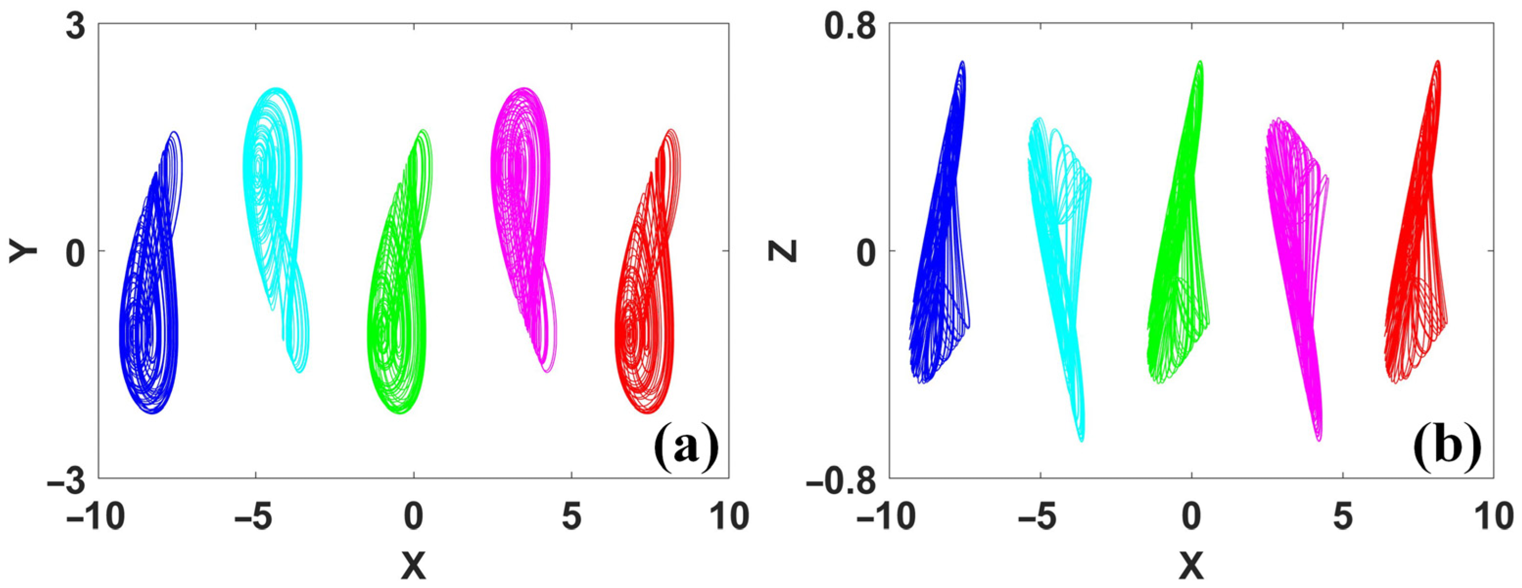
Here, the sinusoidal function of x also brings a new polarity reversal and returns the polarity balance in the last dimension of system (17), thus introducing more coexisting attractors based on periodic offset boosting, as shown in Figure 22. The flexible combinations of offset-boosting-oriented polarity reversal and variable polarity reversal lead to abundant candidates of chaotic systems with infinitely many coexisting attractors or repellors.

5. Symmetry and Elegance in Simple Chaotic Circuits

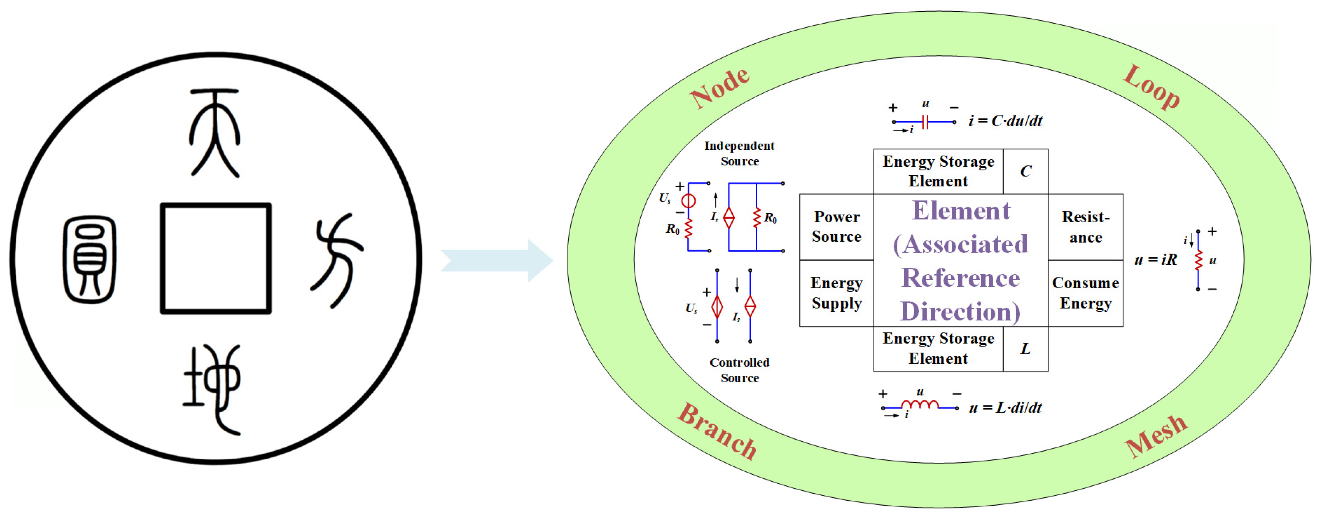
Furthermore, symmetry and conditional symmetry can be seen in nonlinear circuits [90,91,92,93], and in this case, coexisting attractors indicate multiple signal outputting. As we know, the restriction of voltage and current in a circuit is under the rule governed by the structure of circuit topology and the individual characteristic of a circuit component. The structure of circuit topology gives a macro-restriction with the voltage and current, while the individual characteristic of a circuit component leads to a local micro-restriction. The former corresponds to the circuit law of Kirchhoff law, and the latter is related to the local restriction from a circuit element. All the circuit variables must obey the two types of constraints: one is from the topology, and one is from the local specific component. We still see that the local component provides flexibility with the voltage and current constraint because the components vary in many ways. Therefore, using vocabulary from ancient Chinese philosophy, we call these two constraints ‘a square earth with a round sky above’, as shown in Figure 23. The concept of ‘a square earth with a round sky above’ is a philosophical idea in ancient China that is a manifestation of the theory of ‘Yin and Yang’. The sky and circle symbolize movement, but the earth and square represent stillness. In fact, the combination shows a balance of ‘Yin and Yang’ with complementary movement and stillness. The concept of ‘round sky and square earth’ has been shown in ancient Chinese architecture, currency and other aspects, such as the Temple of Heaven, square hole coins and other patterns and structures. In circuits, ‘Sky’ means the fundamental constraint from the ‘Node’ and ‘Loop’. (In fact, they are also combined with ‘Branch’ and ‘Mesh’.) Meanwhile, the ‘Earth’ means the other striction from all kinds of circuit elements. Two kinds of circuit constraints leave much more space for the symmetric evolvement of the circuit system. This special understanding of circuit constraints calls for the insight of circuit design and poses great help for the application of circuit laws.

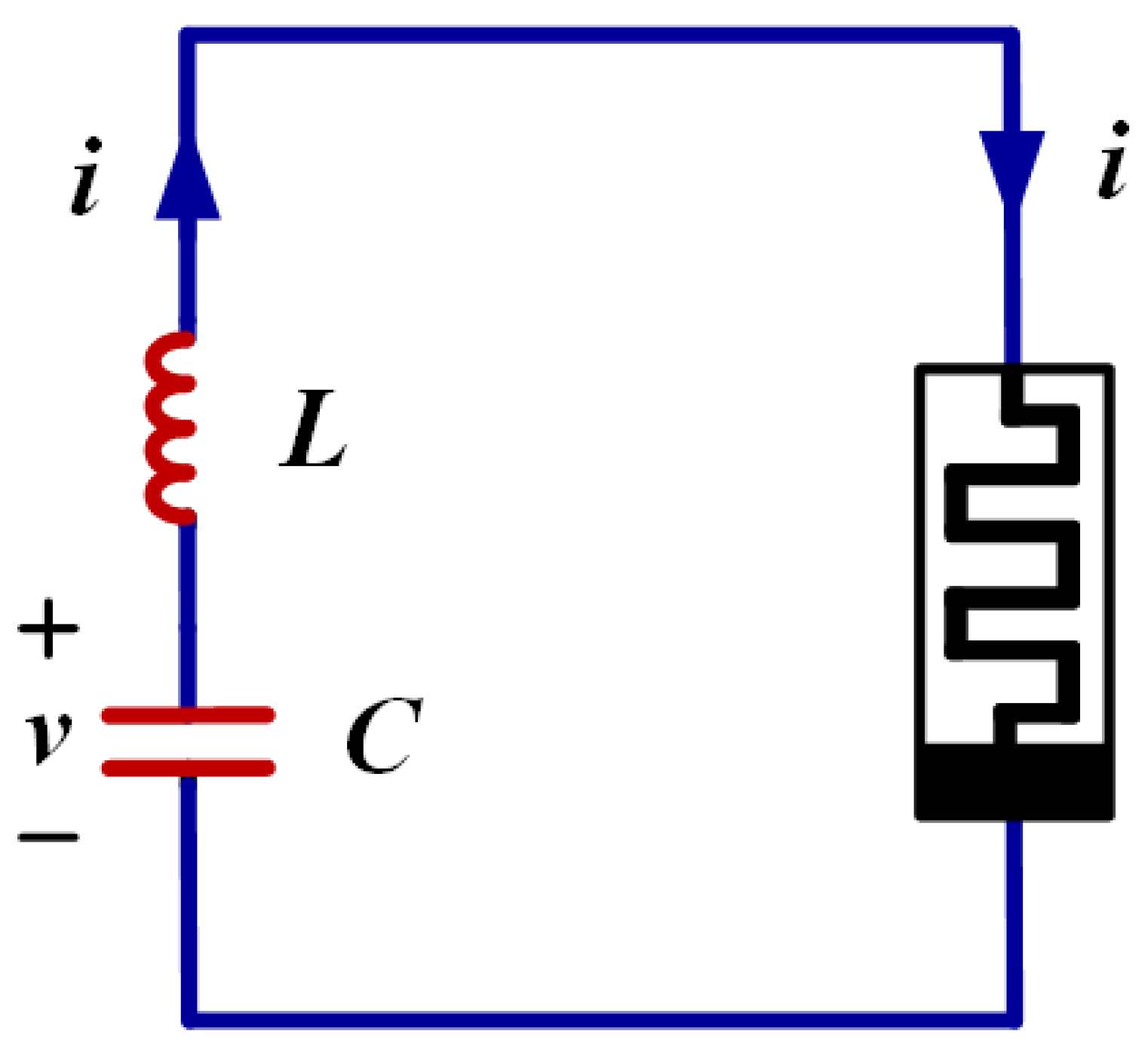
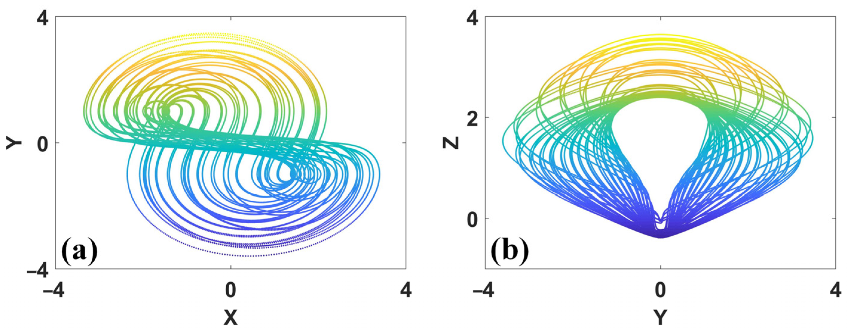
Moreover, in circuits, there are many cases of symmetry and duality. Dynamical behaviors in a chaotic jerk circuit can obtain a smooth symmetry control based on a memristive diode emulator [94]. The effects of symmetry breaking can be seen even in a simple autonomous jerk circuit [95]. Rigorous analyses of windows in a symmetric circuit are revealed in [96]. More observations of symmetry in chaotic systems and circuits are made in [97]. We can enumerate many circuit structures and corresponding circuit laws and see the elegant symmetry or duality, such as capacitive and inductive components, voltage source and current source, series for voltage and parallel for current, series resonance and parallel resonance, the time constant of the resistor and capacitor and the time constant of conduction and inductance. And even more, it seems that the new findings regarding memristors are also associated with the symmetry observation. Furthermore, many circuits of series structure could be transformed to be of parallel structure and give symmetric attractors or coexisting attractors of conditional symmetry. As shown in Figure 24, the simple series circuit [98] including an inductor, a capacitor and a memristor can produce a symmetric chaotic attractor, as shown in Figure 25. The circuit realizes the equation of system (18) with rotational symmetry according to the variables y and z.

$$\{\begin{array}{l}\dot{x}=\alpha (y^2-1),\\ \dot{y}=-\omega z-xy,\\ \dot{z}=\omega y.\end{array}$$

(18)

Conditional symmetry of coexisting attractors can also be generated in a simple parallel circuit structure [99]. The chaotic system (19),

$$\{\begin{array}{l}\dot{x}=\left|y\right|-b,\\ \dot{y}=z,\\ \dot{z}=-az-y+\left|x\right|-c.\end{array}$$

(19)

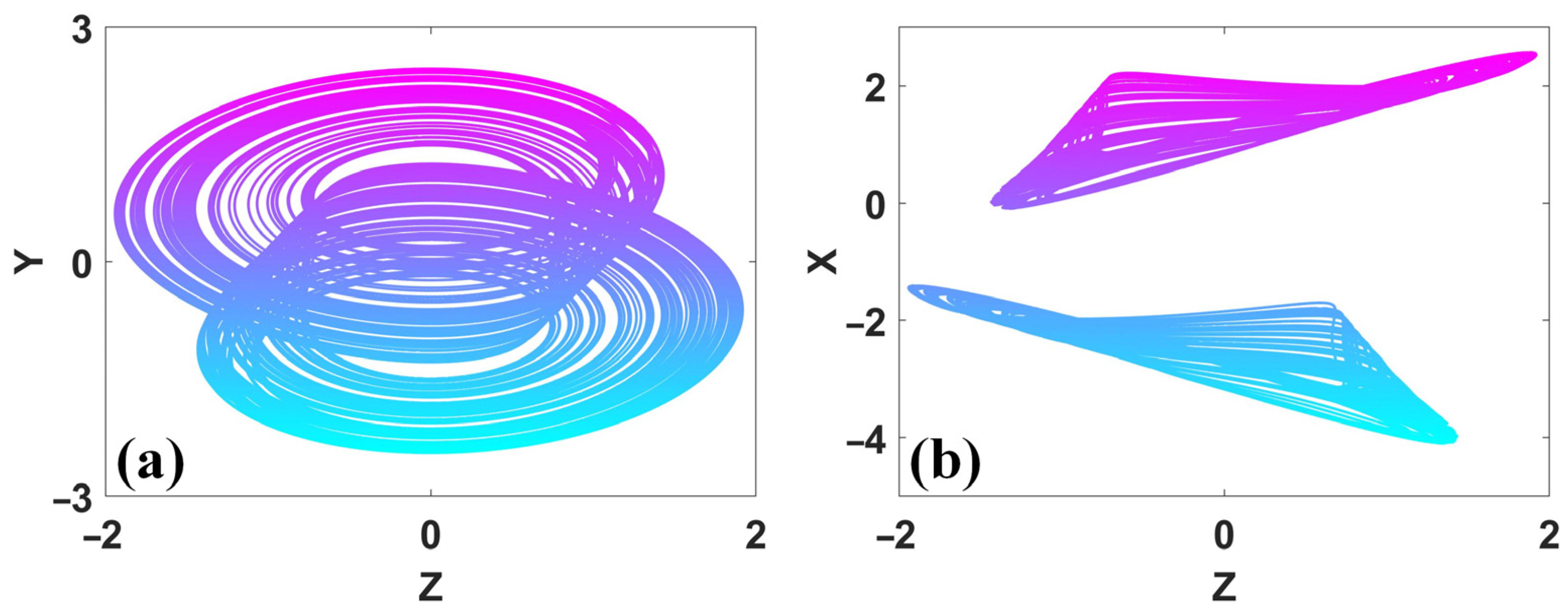
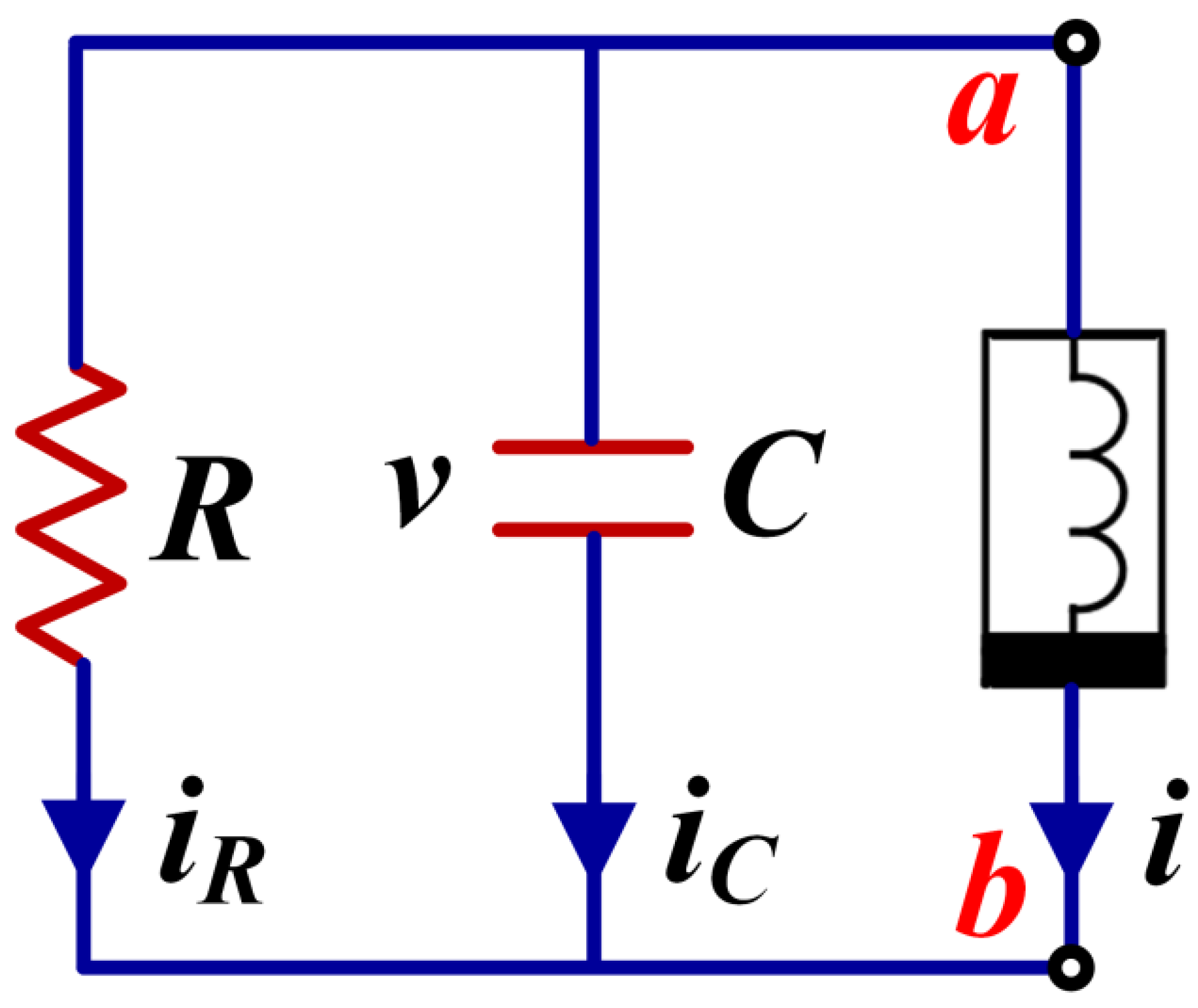
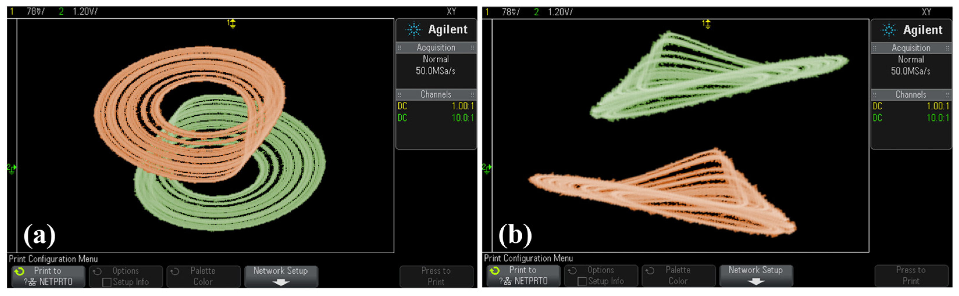
has coexisting chaotic attractors of rotational conditional symmetry when a = 0.6, b = 1, c = 2, as displayed in Figure 26. The structure of system (19) is unique and can be implemented based on a parallel circuit with a capacitor, a resistor and an meminductor, as shown in Figure 27. This simple structure also oscillates outputting two coexisting attractors, as shown in Figure 28. We can declare that people can realize these systems with a dual circuit structure if they want to switch the circuit between the series and parallel.

In fact, the elegant structure or symmetric property of a system does not indicate its simple or easy structure. For example, for doubling the coexisting attractors [63,64,65], let us see system (20),

$$\{\begin{array}{l}\dot{x}=\mathrm{sgn}(x)(c-(b\left|y\right|-1)z),\\ \dot{y}=a{z}^2-yz,\\ \dot{z}=\left|x\right|-d.\end{array}$$

(20)

The coexisting attractors are located in phase space according to the axis of symmetry x = 0. Here, the constant d modifies the distance between two coexisting symmetric attractors. When it increases from d = 4.11 to be d = 8, the distance between those symmetric attractors is also increased, as shown in Figure 29 and Figure 30. Here, the chaotic phase trajectories are elegant and simple, but the circuit for realizing them is not simple. Typically, it is realized based on three lines of operational-amplifier-based integral structure.

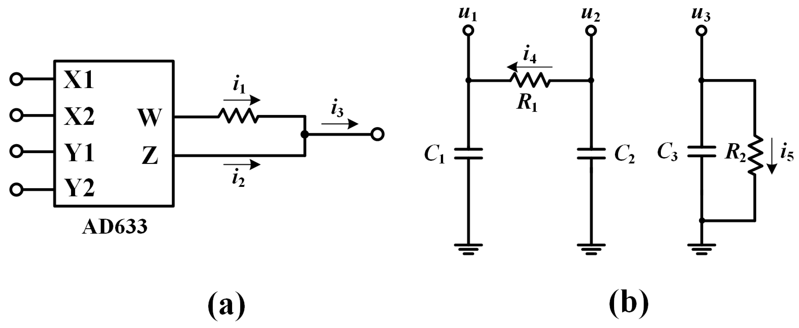
For many of those symmetric chaotic systems, the simple circuit could be constructed by utilizing the inherent characteristics of a multiplier and the differential constraint of the capacitor [100]. As we know, the multiplier AD633 can convert voltage to current with an external resistor. The external voltage transformation characteristic of AD633 obeys the relationship of $\mathrm{W}=\left({\mathrm{X}}_1-{\mathrm{X}}_2\right)\left({\mathrm{Y}}_1-{\mathrm{Y}}_2\right)/10+\mathrm{Z}$. If a resistor connects the output point W and Z in series, as shown in Figure 31a, the output current satisfies $i_2\approx$0 and $i_1\approx i_3$ for a large input resistor of the Z port with a small input current. Thus, the output voltage satisfies the balance of current: $\mathrm{W}=\left({\mathrm{X}}_1-{\mathrm{X}}_2\right)\left({\mathrm{Y}}_1-{\mathrm{Y}}_2\right)/10+\mathrm{W}{-i}_{1}R$. Consequently, the current associated with AD633 is subject to $i_1\approx i_3=\left({\mathrm{X}}_1-{\mathrm{X}}_2\right)\left({\mathrm{Y}}_1-{\mathrm{Y}}_2\right)/10R$. Various combinations of inputs realize those terms with different degrees according to the input variable, and therefore, a multiplier provides the linear terms and quadratic terms for the circuit calculation. Furthermore, the connection of resistor and capacitor drives a flexible integration calculation. When two capacitors are coupled with a resistor as shown in Figure 31b, the current $i_4$ identified by ${(u}_2{-u}_1)/R_1$ equals the current through the capacitor $C_1$ resulting in $\dot{u_1}={(u}_2{-u}_1)/R_1{C}_1$, and similarly leads to the symmetric restraint like $\dot{u_2}={(u}_1{-u}_2)/R_1{C}_2$. When a capacitor and a resistor connect in parallel, the current equation is $\dot{u_3}=-u_3/R_2{C}_3$. From the above two classes of basic circuit constraints, many symmetric chaotic systems with quadratic terms could be implemented in an easy way, like the system written as

$$\{\begin{array}{l}\dot{x}=y-x,\\ \dot{y}=5x-y-xz,\\ \dot{z}=0.5x^2-0.5z.\end{array}$$

(21)

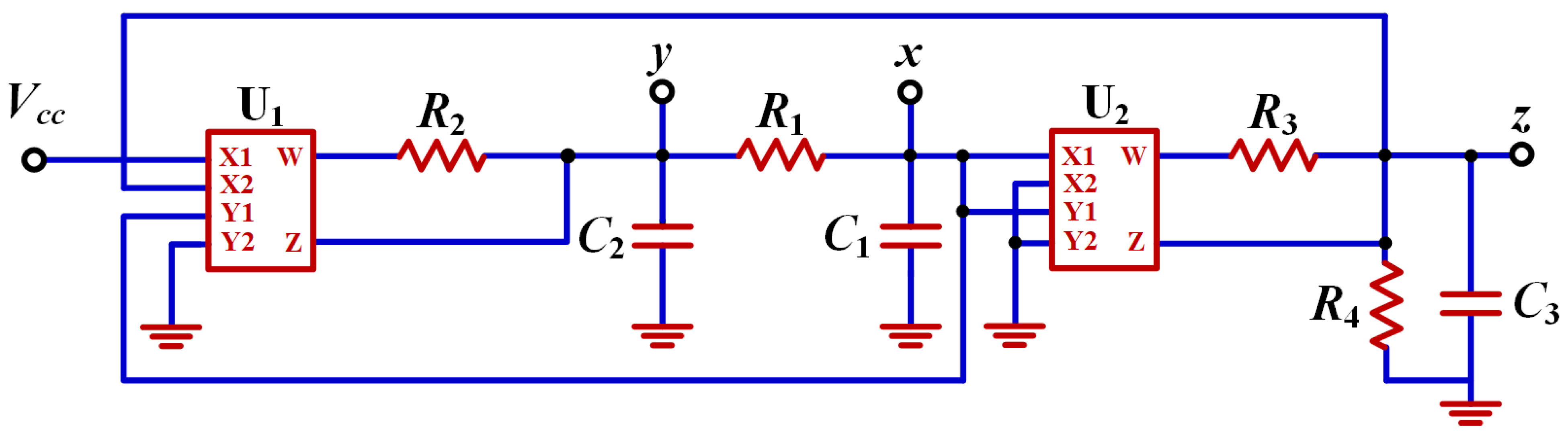
It can be realized with a compact structure, as shown in Figure 32.

6. Conclusions

In the physical world, there are many symmetric systems keeping their stability against the reversal of polarity from some of the dimensions. Symmetric systems provide symmetric solutions, and even when the symmetry is broken, the symmetry turns out to be accompanied by the coexisting symmetric pairs of attractors. More coexisting attractors indicate more freedom of choice for engineering, and sometimes imply more uncertainty and more risks. The observation of symmetry within a dynamical system poses an important suggestive value for fully utilizing the property of symmetry of a practical system. Furthermore, symmetry can be rebuilt, and even can be modified in an imprecise or flexible form. The polarity revision can resort to direct polarity reversals from some of the system variables or be derived by offset boosting with any of the variables. Therefore, a symmetric system can be reconstructed by introducing an absolute-value function and a signum function. More widely, offset boosting can also be employed for rebuilding the chaotic system with conditional symmetry. The structure of a system is not necessarily related to a symmetric or elegant circuit structure. A simple or elegant circuit structure depends on the combinations of modern circuit components.

References

- Lorenz, E.N. Deterministic nonperiodic flow. J. Atmos. Sci. 1963, 20, 130–141. [Google Scholar] [CrossRef]
- Chen, G.; Ueta, T. Yet another chaotic attractor. Int. J. Bifurcat. Chaos 1999, 9, 1465–1466. [Google Scholar] [CrossRef]
- Chua, L.E.; Komuro, M.; Matsumoto, T. The double scroll family. IEEE Trans. Circuits Syst. 1986, 33, 1072–1118. [Google Scholar] [CrossRef] [Green Version]
- Mobayen, S.; Volos, C.; Çavuşoğlu, Ü.; Kaçar, S. A simple chaotic flow with hyperbolic sinusoidal function and its application to voice encryption. Symmetry 2020, 12, 2047. [Google Scholar] [CrossRef]
- Zhang, Z.; Huang, L.; Liu, J.; Guo, Q.; Du, X. A new method of constructing cyclic symmetric conservative chaotic systems and improved offset boosting control. Chaos Solitons Fractals 2022, 158, 112103. [Google Scholar] [CrossRef]
- Khan, J.; Hussain, T.; Mlaiki, N.; Fatima, N. Symmetries of locally rotationally symmetric Bianchi type V spacetime. Results Phys. 2023, 44, 106143. [Google Scholar] [CrossRef]
- Hruda, L.; Kolingerová, I.; Lávička, M.; Maňák, M. Rotational symmetry detection in 3D using reflectional symmetry candidates and quaternion-based rotation parameterization. Comput. Aided Geom. Des. 2022, 98, 102138. [Google Scholar] [CrossRef]
- Boui, A.; Boya, B.F.; Danao, A.A.; Kengne, L.K.; Kengne, J. Control and symmetry breaking aspects of a geomagnetic field inversion model. Chaos 2023, 33, 013139. [Google Scholar] [CrossRef]
- Leutcho, G.D.; Wang, H.; Kengne, R.; Kengne, L.K.; Njitacke, Z.T.; Fozin, T.F. Symmetry-breaking, amplitude control and constant Lyapunov exponent based on single parameter snap flows. Eur. Phys. J. Spec. Top. 2021, 230, 1887–1903. [Google Scholar] [CrossRef]
- Karthikeyan, R.; Jafari, S.; Karthikeyan, A.; Srinivasan, A.; Ayele, B. Hyperchaotic Memcapacitor Oscillator with Infinite Equilibria and Coexisting Attractors. Circuits Syst. Signal Process. 2018, 37, 3702–3724. [Google Scholar]
- Volos, C.K.; Kyprianidis, I.M.; Stouboulos, I.N. Various synchronization phenomena in bidirectionally coupled double scroll circuits. Commun. Nonlinear Sci. Numer. Simul. 2011, 16, 3356–3366. [Google Scholar] [CrossRef]
- Hu, W.; Liu, T.; Han, Z. Dynamical Symmetry Breaking of Infinite-Dimensional Stochastic System. Symmetry 2022, 14, 1627. [Google Scholar] [CrossRef]
- Ramamoorthy, R.; Rajagopal, K.; Leutcho, G.D.; Krejcar, O.; Namazi, H.; Hussain, I. Multistable dynamics and control of a new 4D memristive chaotic Sprott B system. Chaos Solitons Fractals 2022, 156, 111834. [Google Scholar] [CrossRef]
- Bloch, A.M.; Krishnaprasad, P.S.; Marsden, J.E.; Murray, R.M. Nonholonomic mechanical systems with symmetry. Arch. Ration. Mech. Anal. 1996, 136, 21–99. [Google Scholar] [CrossRef] [Green Version]
- Olfati-Saber, R. Normal forms for underactuated mechanical systems with symmetry. IEEE Trans. Autom. Control 2002, 47, 305–308. [Google Scholar] [CrossRef] [Green Version]
- Leonard, N.E.; Marsden, J.E. Stability and drift of underwater vehicle dynamics: Mechanical systems with rigid motion symmetry. Phys. D Nonlinear Phenom. 1997, 105, 130–162. [Google Scholar] [CrossRef] [Green Version]
- Mory, J.F. Oil prices and economic activity: Is the relationship symmetric? Energy J. 1993, 14, 151–161. [Google Scholar] [CrossRef]
- Bischi, G.I.; Gallegati, M.; Naimzada, A. Symmetry-breaking bifurcations and representativefirm in dynamic duopoly games. Ann. Oper. Res. 1999, 89, 252–271. [Google Scholar] [CrossRef]
- Kondepudi, D.K.; Nelson, G.W. Chiral-symmetry-breaking states and their sensitivity in nonequilibrium chemical systems. Phys. A Stat. Mech. Its Appl. 1984, 125, 465–496. [Google Scholar] [CrossRef]
- Piñeros, W.D.; Tlusty, T. Spontaneous chiral symmetry breaking in a random driven chemical system. Nat. Commun. 2022, 13, 2244. [Google Scholar] [CrossRef]
- Kondepudi, D.K.; Nelson, G.W. Chiral symmetry breaking in nonequilibrium chemical systems: Time scales for chiral selection. Phys. Lett. A 1984, 106, 203–206. [Google Scholar] [CrossRef]
- Amit, D.J.; Tsodyks, M.V. Quantitative study of attractor neural networks retrieving at low spike rates: II. Low-rate retrieval in symmetric networks. Netw. Comput. Neural Syst. 1991, 2, 275–294. [Google Scholar] [CrossRef]
- Cho, M.W.; Chun, M.Y. Two symmetry-breaking mechanisms for the development of orientation selectivity in a neural system. J. Korean Phys. Soc. 2015, 67, 1661–1666. [Google Scholar] [CrossRef] [Green Version]
- Meyra, A.G.; Zarragoicoechea, G.J.; Kuz, V.A. Self-organization of plants in a dryland ecosystem: Symmetry breaking and critical cluster size. Phys. Rev. E 2015, 91, 052810. [Google Scholar] [CrossRef]
- Persson, L.; de Roos, A.M. Symmetry breaking in ecological systems through different energy efficiencies of juveniles and adults. Ecology 2013, 94, 1487–1498. [Google Scholar] [CrossRef] [PubMed] [Green Version]
- Dunitz, J.D.; Orgel, L.E. Electronic properties of transition-metal oxides—I: Distortions from cubic symmetry. J. Phys. Chem. Solids 1957, 3, 20–29. [Google Scholar] [CrossRef]
- Berg, R.A.; Wharton, L.; Klemperer, W.; Büchler, A.; Stauffer, J.L. Determination of electronic symmetry by electric deflection: LiO and LaO. J. Chem. Phys. 1965, 43, 2416–2421. [Google Scholar] [CrossRef]
- Renner, R. Symmetry of large physical systems implies independence of subsystems. Nat. Phys. 2007, 3, 645–649. [Google Scholar] [CrossRef] [Green Version]
- Koptsik, V.A. Symmetry principle in physics. J. Phys. C Solid State Phys. 1983, 16, 23. [Google Scholar] [CrossRef]
- Ivanova, I.A.; Leydesdorff, L. Rotational symmetry and the transformation of innovation systems in a Triple Helix of university–industry–government relations. Technol. Forecast. Soc. Chang. 2014, 86, 143–156. [Google Scholar] [CrossRef] [Green Version]
- Daum, S.O.; Hecht, H. Effects of symmetry, texture, and monocular viewing on geographical slant estimation. Conscious. Cogn. 2018, 64, 183–195. [Google Scholar] [CrossRef] [PubMed]
- Hammond, K.R.; Mumpower, J.L.; Smith, T.H. Linking environmental models with models of human judgment: A symmetrical decision aid. IEEE Trans. Syst. Man Cybern. 1977, 7, 358–367. [Google Scholar] [CrossRef]
- Turvey, M.T.; Shaw, R.E. Ecological foundations of cognition. I: Symmetry and specificity of animal-environment systems. J. Conscious. Stud. 1999, 6, 95–110. [Google Scholar]
- Shilnikov, L.P.; Shilnikov, A.L.; Turaev, D.V.; Chua, L.O. Methods of Qualitative Theory in Nonlinear Dynamics, Part 2; World-Scientific: Singapore, 2009. [Google Scholar]
- Shil’nikov, A.L. On bifurcations of the Lorenz attractor in the Shimizu-Morioka model. Phys. D Nonlinear Phenom. 1993, 62, 338–346. [Google Scholar] [CrossRef]
- Grassi, G.; Severance, F.L.; Miller, D.A. Multi-wing hyperchaotic attractors from coupled Lorenz systems. Chaos Solitons Fractals 2009, 41, 284–291. [Google Scholar] [CrossRef]
- Yu, S.; Tang, W.K.; Lu, J.; Chen, G. Generation of n × m wing Lorenz-Like attractors from a modified Shimizu–Morioka model. IEEE Trans. Circuits Syst. II Express Briefs 2008, 55, 1168–1172. [Google Scholar] [CrossRef]
- Chang, H.; Li, Y.; Chen, G. A novel memristor-based dynamical system with multi-wing attractors and symmetric periodic bursting. Chaos 2020, 30, 043110. [Google Scholar] [CrossRef] [Green Version]
- Loskutov, A.Y. Dynamical chaos: Systems of classical mechanics. Phys.-Uspekhi 2007, 50, 939. [Google Scholar] [CrossRef]
- Smale, S. Diffeomorphisms with many periodic points. Matematika 1967, 11, 88–106. [Google Scholar]
- Anosov, D.V.; Sinai, Y.G. Some smooth ergodic systems. Russ. Math. Surv. 1967, 22, 103. [Google Scholar] [CrossRef]
- Guan, Z.H.; Huang, F.; Guan, W. Chaos-based image encryption algorithm. Phys. Lett. A 2005, 346, 153–157. [Google Scholar] [CrossRef]
- Zheng, J.; Hu, H. A symmetric image encryption scheme based on hybrid analog-digital chaotic system and parameter selection mechanism. Multimed. Tools Appl. 2021, 80, 20883–20905. [Google Scholar] [CrossRef]
- Chen, G.; Mao, Y.; Chui, C.K. A symmetric image encryption scheme based on 3D chaotic cat maps. Chaos Solitons Fractals 2004, 21, 749–761. [Google Scholar] [CrossRef]
- Radwan, A.G.; AbdElHaleem, S.H.; Abd-El-Hafiz, S.K. Symmetric encryption algorithms using chaotic and non-chaotic generators: A review. J. Adv. Res. 2016, 7, 193–208. [Google Scholar] [CrossRef] [PubMed] [Green Version]
- Mokhnache, S.; Daachi, M.E.H.; Bekkouche, T.; Diffellah, N. A Combined Chaotic System for Speech Encryption. Eng. Technol. Appl. Sci. Res. 2022, 12, 8578–8583. [Google Scholar] [CrossRef]
- Sathiyamurthi, P.; Ramakrishnan, S. Speech encryption using hybrid-hyper chaotic system and binary masking technique. Multimed. Tools Appl. 2022, 81, 6331–6349. [Google Scholar] [CrossRef]
- Ashtiyani, M.; Birgani, P.M.; Madahi, S. Speech signal encryption using chaotic symmetric cryptography. J. Basic. Appl. Sci. Res. 2012, 2, 1678–1684. [Google Scholar]
- Yu, F.; Li, L.; Tang, Q.; Cai, S.; Song, Y.; Xu, Q. A survey on true random number generators based on chaos. Discret. Dyn. Nat. Soc. 2019, 2019, 2545123. [Google Scholar] [CrossRef]
- Koyuncu, I.; Özcerit, A.T. The design and realization of a new high speed FPGA-based chaotic true random number generator. Comput. Electr. Eng. 2017, 58, 203–214. [Google Scholar] [CrossRef]
- Sprott, J.C. Simplest chaotic flows with involutional symmetries. Int. J. Bifurcat. Chaos 2014, 24, 1450009. [Google Scholar] [CrossRef]
- Li, C.; Sprott, J.C. Coexisting hidden attractors in a 4-D simplified Lorenz system. Int. J. Bifurcat. Chaos 2014, 24, 1450034. [Google Scholar] [CrossRef]
- Wang, X.; Wang, M. A hyperchaos generated from Lorenz system. Phys. A Stat. Mech. Its Appl. 2008, 387, 3751–3758. [Google Scholar] [CrossRef]
- Barboza, R.U.Y. Dynamics of a hyperchaotic Lorenz system. Int. J. Bifurcat. Chaos 2007, 17, 4285–4294. [Google Scholar] [CrossRef]
- Li, C.; Sprott, J.C. Variable-boostable chaotic flows. Optik 2016, 127, 10389–10398. [Google Scholar] [CrossRef]
- Ma, C.; Mou, J.; Xiong, L.; Banerjee, S.; Liu, T.; Han, X. Dynamical analysis of a new chaotic system: Asymmetric multistability, offset boosting control and circuit realization. Nonlinear Dyn. 2021, 103, 2867–2880. [Google Scholar] [CrossRef]
- Leutcho, G.D.; Kengne, J. A unique chaotic snap system with a smoothly adjustable symmetry and nonlinearity: Chaos, offset-boosting, antimonotonicity, and coexisting multiple attractors. Chaos Solitons Fractals 2018, 113, 275–293. [Google Scholar] [CrossRef]
- Xu, C.; Ur Rahman, M.; Baleanu, D. On fractional-order symmetric oscillator with offset-boosting control. Nonlinear Anal. Model. Control 2022, 27, 994–1008. [Google Scholar] [CrossRef]
- Gu, S.; He, S.; Wang, H.; Du, B. Analysis of three types of initial offset-boosting behavior for a new fractional-order dynamical system. Chaos Solitons Fractals 2021, 143, 110613. [Google Scholar] [CrossRef]
- Sayed, W.S.; Roshdy, M.; Said, L.A.; Radwan, A.G. Design and FPGA verification of custom-shaped chaotic attractors using rotation, offset boosting and amplitude control. IEEE Trans. Circuits Syst. II Express Briefs 2021, 68, 3466–3470. [Google Scholar] [CrossRef]
- Bayani, A.; Rajagopal, K.; Khalaf, A.J.M.; Jafari, S.; Leutcho, G.D.; Kengne, J. Dynamical analysis of a new multistable chaotic system with hidden attractor: Antimonotonicity, coexisting multiple attractors, and offset boosting. Phys. Lett. A 2019, 383, 1450–1456. [Google Scholar] [CrossRef]
- Leutcho, G.D.; Kengne, J.; Kengne, R. Remerging Feigenbaum trees, and multiple coexisting bifurcations in a novel hybrid diode-based hyperjerk circuit with offset boosting. Int. J. Dyn. Control 2019, 7, 61–82. [Google Scholar] [CrossRef]
- Li, C.; Wang, R.; Ma, X.; Jiang, Y.; Liu, Z. Embedding any desired number of coexisting attractors in memristive system. Chin. Phys. B 2021, 30, 120511. [Google Scholar] [CrossRef]
- Li, C.; Lu, T.; Chen, G.; Xing, H. Doubling the coexisting attractors. Chaos 2019, 29, 051102. [Google Scholar] [CrossRef] [PubMed]
- Wang, R.; Li, C.; Kong, S.; Jiang, Y.; Lei, T. A 3D memristive chaotic system with conditional symmetry. Chaos Solitons Fractals 2022, 158, 111992. [Google Scholar] [CrossRef]
- Rössler, O.E. An equation for continuous chaos. Phys. Lett. A 1976, 57, 397–398. [Google Scholar] [CrossRef]
- Letellier, C.; Dutertre, P.; Maheu, B. Unstable periodic orbits and templates of the Rössler system: Toward a systematic topological characterization. Chaos 1995, 5, 271–282. [Google Scholar] [CrossRef]
- Rafikov, M.; Balthazar, J.M. On an optimal control design for Rössler system. Phys. Lett. A 2004, 333, 241–245. [Google Scholar] [CrossRef]
- Li, C.; Sun, J.; Lu, T.; Lei, T. Symmetry evolution in chaotic system. Symmetry 2020, 12, 574. [Google Scholar] [CrossRef] [Green Version]
- Li, C.; Sun, J.; Sprott, J.C.; Lei, T. Hidden attractors with conditional symmetry. Int. J. Bifurcat. Chaos 2020, 30, 2030042. [Google Scholar] [CrossRef]
- Gu, Z.; Li, C.; Iu, H.H.; Min, F.; Zhao, Y. Constructing hyperchaotic attractors of conditional symmetry. Eur. Phys. J. B 2019, 92, 221. [Google Scholar] [CrossRef]
- Lu, T.; Li, C.; Jafari, S.; Min, F. Controlling coexisting attractors of conditional symmetry. Int. J. Bifurcat. Chaos 2019, 29, 1950207. [Google Scholar] [CrossRef]
- Li, C.; Sprott, J.C.; Xing, H. Constructing chaotic systems with conditional symmetry. Nonlinear Dyn. 2017, 87, 1351–1358. [Google Scholar] [CrossRef]
- Li, C.; Sprott, J.C.; Liu, Y.; Gu, Z.; Zhang, J. Offset boosting for breeding conditional symmetry. Int. J. Bifurcat. Chaos 2018, 28, 1850163. [Google Scholar] [CrossRef]
- Li, C.; Sprott, J.C.; Zhang, X.; Chai, L.; Liu, Z. Constructing conditional symmetry in symmetric chaotic systems. Chaos Solitons Fractals 2022, 155, 111723. [Google Scholar] [CrossRef]
- Li, C.; Xu, Y.; Chen, G.; Liu, Y.; Zheng, J. Conditional symmetry: Bond for attractor growing. Nonlinear Dyn. 2019, 95, 1245–1256. [Google Scholar] [CrossRef]
- Jia, L.L.; Lai, B.C. A new continuous memristive chaotic system with multistability and amplitude control. Eur. Phys. J. Plus 2022, 137, 604. [Google Scholar] [CrossRef]
- Wu, Q.; Hong, Q.; Liu, X.; Wang, X.; Zeng, Z. A novel amplitude control method for constructing nested hidden multi-butterfly and multiscroll chaotic attractors. Chaos Solitons Fractals 2020, 134, 109727. [Google Scholar] [CrossRef]
- Wang, X.; Deng, L.; Zhang, W. Hopf bifurcation analysis and amplitude control of the modified Lorenz system. Appl. Math. Comput. 2013, 225, 333–344. [Google Scholar] [CrossRef]
- Liu, Z.; Lai, Q. A novel memristor-based chaotic system with infinite coexisting attractors and controllable amplitude. Indian J. Phys. 2023, 97, 1159–1167. [Google Scholar] [CrossRef]
- Moon, S.; Baik, J.J.; Hong, S.H. Coexisting attractors in a physically extended Lorenz system. Int. J. Bifurcat. Chaos 2021, 31, 2130016. [Google Scholar] [CrossRef]
- Boya, B.F.B.A.; Ramakrishnan, B.; Effa, J.Y.; Kengne, J.; Rajagopal, K. The effects of symmetry breaking on the dynamics of an inertial neural system with a non-monotonic activation function: Theoretical study, asymmetric multistability and experimental investigation. Phys. A Stat. Mech. Its Appl. 2022, 602, 127458. [Google Scholar] [CrossRef]
- Yan, S.; Sun, X.; Wang, Q.; Ren, Y.; Shi, W.; Wang, E. A novel double-wing chaotic system with infinite equilibria and coexisting rotating attractors: Application to weak signal detection. Phys. Scr. 2021, 96, 125216. [Google Scholar] [CrossRef]
- Li, C.; Sprott, J.C.; Liu, Y. Time-reversible chaotic system with conditional symmetry. Int. J. Bifurcat. Chaos 2020, 30, 2050067. [Google Scholar] [CrossRef]
- Lai, Q.; Kuate, P.D.K.; Liu, F.; Iu, H.H.C. An extremely simple chaotic system with infinitely many coexisting attractors. IEEE Trans. Circuits Syst. II Express Briefs 2019, 67, 1129–1133. [Google Scholar] [CrossRef]
- Wu, H.; Bao, H.; Xu, Q.; Chen, M. Abundant coexisting multiple attractors’ behaviors in three-dimensional sine chaotic system. Complexity 2019, 2019, 3687635. [Google Scholar] [CrossRef]
- Volos, C.; Akgul, A.; Pham, V.T.; Stouboulos, I.; Kyprianidis, I. A simple chaotic circuit with a hyperbolic sine function and its use in a sound encryption scheme. Nonlinear Dyn. 2017, 89, 1047–1061. [Google Scholar] [CrossRef]
- Hu, X.; Sang, B.; Wang, N. The chaotic mechanisms in some jerk systems. AIMS Math. 2022, 7, 15714–15740. [Google Scholar] [CrossRef]
- Karawanich, K.; Kumngern, M.; Chimnoy, J.; Prommee, P. A four-scroll chaotic generator based on two nonlinear functions and its telecommunications cryptography application. AEU Int. J. Electron. Commun. 2022, 157, 154439. [Google Scholar] [CrossRef]
- Qiu, H.; Xu, X.; Jiang, Z.; Sun, K.; Cao, C. Dynamical behaviors, circuit design, and synchronization of a novel symmetric chaotic system with coexisting attractors. Sci. Rep. 2023, 13, 1893. [Google Scholar] [CrossRef]
- Wang, Z.; Liu, S. Design and implementation of simplified symmetry chaotic circuit. Symmetry 2022, 14, 2299. [Google Scholar] [CrossRef]
- Kengne, J.; Mogue, R.L.T.; Fozin, T.F.; Telem, A.N.K. Effects of symmetric and asymmetric nonlinearity on the dynamics of a novel chaotic jerk circuit: Coexisting multiple attractors, period doubling reversals, crisis, and offset boosting. Chaos Solitons Fractals 2019, 121, 63–84. [Google Scholar] [CrossRef]
- Kahlert, C. The effects of symmetry breaking in Chua’s circuit and related piecewise-linear dynamical systems. Int. J. Bifurcat. Chaos 1993, 3, 963–979. [Google Scholar] [CrossRef]
- Kamdem Tchiedjo, S.; Kamdjeu Kengne, L.; Kengne, J.; Djuidje Kenmoe, G. Dynamical behaviors of a chaotic jerk circuit based on a novel memristive diode emulator with a smooth symmetry control. Eur. Phys. J. Plus 2022, 137, 940. [Google Scholar] [CrossRef]
- Kengne, L.K.; Kengne, J.; Fotsin, H.B. The effects of symmetry breaking on the dynamics of a simple autonomous jerk circuit. Analog. Integr. Circuits Signal Process. 2019, 101, 489–512. [Google Scholar] [CrossRef]
- Nishio, Y.O.; Inaba, N.A.; Mori, S.H.; Saito, T.O. Rigorous analyses of windows in a symmetric circuit. IEEE Trans. Circuits Syst. 1990, 37, 473–487. [Google Scholar] [CrossRef]
- Volos, C. Symmetry in Chaotic Systems and Circuits. Symmetry 2022, 14, 1612. [Google Scholar] [CrossRef]
- Itoh, M.; Chua, L.O. Memristor hamiltonian circuits. Int. J. Bifurcat. Chaos 2011, 21, 2395–2425. [Google Scholar] [CrossRef]
- Jiang, Y.; Li, C.; Zhang, C.; Lei, T.; Jafari, S. Constructing meminductive chaotic oscillator. IEEE Trans. Circuits Syst. II Express Briefs 2023, 70, 2675–2679. [Google Scholar] [CrossRef]
- Wu, J.; Li, C.; Ma, X.; Lei, T.; Chen, G. Simplification of chaotic circuits with quadratic nonlinearity. IEEE Trans. Circuits Syst. II Express Briefs 2021, 69, 1837–1841. [Google Scholar] [CrossRef]
Figure 1.
Symmetry, asymmetry and conditional symmetry in chaotic systems.
Figure 2.
Attractor of rotational symmetry in system (1) when σ = 0.279, r = 0, b = −0.3 and IC = (−0.1, 0.1, −2): (a) x–y, (b) x–z.
Figure 3.
Symmetric solutions under the broken symmetry.
Figure 4.
Symmetric pair of attractors with rotational symmetry in system (1) under the parameters σ = 0.256, r = 0, b = −0.3 and IC1 = (−0.1, 0.1, −2) (left), IC2 = (0.1, −0.1, −2) (right): (a) x–y, (b) x–z.
Figure 5.
Coexisting strange attractors of system (1) with rotational symmetry when σ = 0.279, r = 0, b = −0.3 and IC1 = (−0.1, 0.1, −2) (blue), IC2 = (−0.1, 0.1, −14) (cyan), IC3 = (0.1, −0.1, −14) (purple): (a) x–y, (b) x–z.
Figure 6.
Symmetric attractor of inversion symmetry in system (2) when a = 1.7, b = 2 and IC = (1, 0, 0): (a) x–y, (b) x–z.
Figure 7.
A symmetric pair of coexisting attractors in system (2) when a = 2.1, b = 2 and IC1 = (−1, 0, 0) (left), IC2 = (1, 0, 0) (right): (a) x–y, (b) x–z.
Figure 8.
Attractor of reflection invariant system (3) with a = 0.35 and IC = (−2, 2, 0): (a) x–y, (b) x–z.
Figure 9.
A symmetric pair of attractors in a reflection invariant system (3) with a = 0.7 and IC1 = (−2, 2, 0) (cyan), IC2 = (2, 2, 0) (purple): (a) x–y, (b) x–z.
Figure 10.
Quasi-periodic torus coexisting with a symmetric pair of chaotic attractors at a = 6, b = 0.1 (red and blue attractors correspond to two symmetric initial conditions under IC = (0, ±4, 0, ±5), cyan is for symmetric torus under IC = (1, −1, 1, −1)): (a) x–z, (b) y–z.
Figure 11.
Symmetric attractors of system (8) with a = b = 0.2, c = 6.5, d = 0 and IC1 = (−9, 0, 2) (up), IC2 = (−9, 0, −2) (down): (a) x–z, (b) y–z.
Figure 12.
Symmetric attractors of system (8) with a = b = 0.2, c = 6.5, d = 12 and IC1 = (−9, 0, 12) (up), IC2 = (−9, 0, −12) (down): (a) x–z, (b) y–z.
Figure 13.
Eight coexisting attractors of system (9) with a = b = 0.2, c = 6.5, d1 = 11, d2 = 13, d3 = 12.
Figure 14.
Polarity balance in a dynamical system.
Figure 15.
Coexisting conditional reflection symmetric attractors of system (10) with IC1 = (3, −1.5, −2) (red), IC2 = (3, −1.5, 1) (green): (a) x–z, (b) y–z.
Figure 16.
Coexisting conditional rotational symmetric attractors of system (11) with IC1 = (3, 1, 0.5) (red), IC2 = (−3, 1, 0.5) (green): (a) x–y, (b) x–z.
Figure 17.
Coexisting attractors in system (12) by 2D offset boosting, when a = 0.22 and IC1 = (2, 6, −1) (red), IC2 = (−1, 1, −1) (green): (a) x–z, (b) y–z.
Figure 18.
Coexisting conditional rotational symmetric attractors of system (13) with a = 0.35, IC1 = (0, 0.4, 6) (red), IC2 = (0, 0.4, −5) (green): (a) x–z, (b) y–z.
Figure 19.
Coexisting attractors in conditional symmetric system (14) with a = 0.4, b = 1, IC1 = (0, 14, 17) (red), IC2 = (0, −6, −7) (green): (a) x–y, (b) x–z.
Figure 20.
Coexisting attractors in symmetric system (15) with IC1 = (1, 5, 5.5) (red), IC2 = (1, −5, −4.5) (green): (a) x–z, (b) y–z.
Figure 21.
Coexisting repellors with conditional symmetry in system (16): (a) y–x, (b) z–x. (IC = (0, 0.96, 0) is red, IC = (6, 2, 2) is yellow, IC = (0, −0.96, 0) is green, IC = (−6, −2, −2) is blue).
Figure 22.
Coexisting attractors in system (17): (a) x–y, (b) x–z. (IC = (1, 0, 0) is green, IC = (1 + 1.25π, 0, 0) is pink, IC = (1 + 2.5π, 0, 0) is red, IC = (1−1.25π, 0, 0) is cyan, IC = (1−2.5π, 0, 0) is blue).
Figure 23.
‘A square earth with a round sky above’ and two types of circuit constraints.
Figure 24.
A simple series chaotic circuit with a memristor, an inductor and a capacitor.
Figure 25.
Symmetric attractor in system (18) with α = 1, ω = 1 and IC = (4.1, 0.7, 5): (a) x–y, (b) y–z.
Figure 26.
Conditional symmetric chaotic attractors of system (19) with a = 0.6, b = 1, c = 2, (a) z–y, (b) z–x. (IC = (2, 0, −1) is up, IC = (−2, 0, 1) is down).
Figure 27.
Meminductive parallel chaotic circuit for realizing system (19).
Figure 28.
Conditional symmetric chaotic attractors of system (19) with a = 0.6, b = 1, c = 2 observed in oscilloscope, (a) z–y, (b) z–x. (IC = (2, 0, −1) is green, IC = (−2, 0, 1) is brown).
Figure 29.
Chaotic attractors in system (20) with a = 0.6, b = 1, c = 1, d = 4.11 and IC = (1, 1, −1). Here, two coexisting attractors close each other and bond to be a pseudo-double-scroll attractor: (a) x–y, (b) x–z.
Figure 30.
Coexisting attractors of system (20) with a = 0.6, b = 1, c = 1, d = 8: (a) x–y, (b) x–z. (IC = (−1, 1, −1) is left, IC = (1, 1, −1) is right).
Figure 31.
Simple circuit operation unit: (a) multiplier current constraint under external resistance, (b) the resistor-capacitor coupling realizes current control.
Figure 32.
Schematic circuit of the system (21).