
Enhanced Dispersion Monitoring Structures Based on Modified Successive Sampling: Application to Fertilizer Production Process


1
Department of Economics and Statistics, Dr Hasan Murad School of Management (HSM), University of Management and Technology, Lahore 54770, Pakistan
2
Department of Statistics, Virtual University of Pakistan, Lahore 54000, Pakistan
3
Industrial and Systems Engineering Department, King Fahd University of Petroleum and Minerals, Dhahran 31261, Saudi Arabia
4
Centre for Smart Mobility and Logistics, King Fahd University of Petroleum and Minerals, Dhahran 31261, Saudi Arabia
5
Department of Mathematics, King Fahd University of Petroleum and Minerals, Dhahran 31261, Saudi Arabia
*
Author to whom correspondence should be addressed.
Symmetry 2023, 15(5), 1108; https://doi.org/10.3390/sym15051108
Submission received: 13 April 2023
/
Revised: 12 May 2023
/
Accepted: 16 May 2023
/
Published: 18 May 2023
(This article belongs to the Special Issue Mathematical Models and Methods in Various Sciences)
Abstract
:In this era of Industry 4.0, efficient and affordable monitoring solutions are needed for the surveillance of manufacturing/service operations. In general, memory-type control charts outperform memoryless control charts when it comes to determining the changes in location and dispersion parameters of symmetrically distributed processes. Before monitoring the process location, it is essential to monitor the process dispersion, since the latter presumes that the process variance remains stable. In practice, the modified successive sampling (MSS) mechanism is preferred over simple random sampling for its cost-effectiveness and efficiency. This study was designed in order to propose moving average and double moving average control charts based on the MSS mechanism for monitoring the dispersion parameter. The performance of the proposed charts is evaluated using run-length measures, and a comparison is made with an existing control chart based on MSS and repetitive sampling. Furthermore, the application of the designed moving and double moving average charts is demonstrated using a case study related to fertilizer production. It is observed that the proposed double moving average control chart performs better than the other control charts designed under the MSS and repetitive sampling schemes.
1. Introduction
In statistical process control (SPC), a control chart is the most important and frequently used tool to monitor process parameters (such as location and/or dispersion). Quality practitioners mostly prefer using control charts to identify sustainable variations in the process parameters. In a process, the main application of control charts is the visual detection of unusual variations for which educative action is needed to move the process back into the in-control (IC) state [1]. Shewhart [2] invented the first control chart, named the Shewhart chart, which was designed based on a current sample. Therefore, Shewhart-type (memoryless) control charts are more efficient for detecting large shifts in the process and are less efficient for detecting shifts of small magnitude. On the other hand, memory-type control charts, such as cumulative sum (CUSUM) by Page [3], exponentially weighted moving average (EWMA) by Roberts [4], moving average (MA) by Wong et al. [5] and double moving average (DMA) by [6], perform more efficiently for the timely detection of small shifts in the process. The reason for this is that their structures are based on current as well as past observations of the process [7].
Many quality practitioners have studied MA and DMA control charts in detail. MA and combined MA-Shewhart design procedures were designed by Wong et al. [5]. To monitor both process parameters (mean and variance), Khoo and Yap [8] designed an MA chart for the joint monitoring of both upwards and downwards shift. For the monitoring of process variability, Adeoti et al. [9] designed a double moving average-S chart that detects small to moderate shifts. Khoo and Wong [10] presented a double exponentially weighted moving average (DEWMA) chart to monitor the location parameter of a process. For monitoring defective products, Areepong [11] explicated formulas for the average run length (ARL) of an MA chart, and Phant et al. [12] gave an expression for the ARL of a DMA chart under the integer-valued autoregression of order one (INAR(1)) processes. Adeoti et al. [9] and Alevizakos et al. [6] studied a double moving average (DMA) chart to enhance the detection ability of a moving average (MA) chart under normal distribution and assuming a simple random sampling (SRS) mechanism.
In the literature, many studies have presented more accurate and efficient estimators, some of which use sampling schemes other than SRS. Their findings reveal that such sampling mechanisms are more reliable, time- and cost-effective as compared to SRS. Salazar and Sinha [13] designed memoryless control charts using ranked set sampling (RSS). Al-Nasser and Al-Rawwash [14] developed Shewhart control charts based on a robust RSS mechanism. Abujiya et al. [15] suggested an EWMA structure based on median RSS, while Munir and Haq [16] presented a CUSUM structure using an ordered and double ordered RSS scheme. For location monitoring, Nawaz et al. [17], Nawaz and Han [18] and Hussain et al. [19] studied different median- and mean-based Shewhart, CUSUM, EWMA and homogeneously weighted moving average (HWMA) charts under ranked set sampling (RSS) and neoteric ranked set sampling (NRSS) schemes. Reynolds Jr and Lou [20] evaluated a GLR control chart for the monitoring of process mean. The generalized control chart is based on the likelihood ratio of normal distribution under SRS. The average time to signal measure is used to evaluate the performance of the proposed charts. A comparison with the Shewhart, CUSUM and the combined Shewhart-CUSUM charts is provided. Furthermore, Sheriff et al. [21] performed a comparative study on PCA-based GLR control charts for process monitoring. Their method is based on the likelihood ratio of principal component analysis for high-dimensional data. The proposed chart is used to monitor location and/or dispersion shifts. Riaz et al. [22] designed a new HWMA control chart for the monitoring of the dispersion parameter using wind farm data. Anwar et al. [23] and Anwar et al. [24] proposed mixed memory-type control charts for the simultaneous monitoring of more than one parameters using auxiliary information. A double generally weighted moving average (GWMA) control chart for monitoring dispersion parameters was designed by Alevizakos et al. [25]. Akhtar et al. [26] evaluated the EWMA control chart by using log-normal distributions with estimated parameters to monitor process variability. A GWMA maximum chart for joint monitoring was designed by Chatterjee et al. [27]. Similarly, Chatterjee et al. [28] introduced an efficient control charting structure named double GWMA (DGWMA) for the monitoring of location and dispersion parameters. Khan et al. [29] developed a hybrid EWMA control chart based on a ranked set sampling scheme under a Bayesian approach using hard-bake process data. For the monitoring of variability in a process, an exponentially weighted moving average control chart based on generalized fast initial response was designed by Ajibade et al. [30]. Recently, a new weighted adaptive CUSUM chart using a bivariate normal process to monitor generalized variance was proposed by Haq and Abbasi [31].
All these aforementioned studies under the Shewhart setup and their analyses are conducted under the assumption that all sample observations are available and no information from the previous sample(s) is used for making decisions. The CUSUM and EWMA structures overcome this issue partially by defining the plotting statistics as functions of current and previous samples. There are many practical situations in which it is desirable to conduct control charting analysis with a sample size but only observations are available at each time point, where is a positive integer. For such situations, a cost-effective and time-saving sampling procedure named modified successive sampling (MSS) was first introduced by Yaqub et al. [32]. Yaqub et al. [32] and Abbas et al. [33] proposed Shewhart charts based on MSSS schemes for the detection of location and dispersion parameters, respectively. The modified form of the successive sampling scheme is more effective than other existing sampling techniques and is specially designed to monitor process parameters (location or dispersion). For the real-time surveillance of the location parameter, memory-type control charts based on MSS were designed by Hyder et al. [34].
The situation of a reduced sample size can also occur in the case of dispersion monitoring. To the best of our knowledge, there are no studies in the literature that provide a solution for such situations under memory-type structures. Filling this research gap, the current study is focused on designing efficient memory-type control charts (MA-, DMA-) based on the MSS scheme for the monitoring of symmetrical process variability. The performance of the designed control charts is compared with the existing Shewhart chart for process dispersion monitoring under various MSS schemes.
The rest of this article is organized as follows. In Section 2, a summary of MSS schemes is given, along with the construction of the designed charts based on these schemes. Section 3 presents the performance of proposed charts, which is evaluated through simulations. A comparative analysis is presented in Section 4, Section 5 illustrates the implementation of the designed charts using real-life data and the concluding remarks of the article and future recommendations are given in Section 6.
2. Methodology
This section briefly defines the structure and several schemes of MSS. Additionally, for the efficient monitoring framework of the scale parameter, we construct MA- and DMA- charts based on MSS in this section.
2.1. Modified Successive Sampling
The timely inspection of defective items may improve the cost-efficiency of any industrial process. To improve cost-efficiency, Jessen [35] developed the successive sampling technique for various inventory problems. However, in most surveys, SRS is suggested for a single occasion. However, an item’s quality is regularly examined in industrial practices. Therefore, to obtain reliable estimates, successive sampling plays an important role in such repeated assessments. The structure of successive sampling is that the initial sample is selected on the 1st occasion and the next sample (having some sample points from the previous sample) is drawn on the 2nd occasion, and so on. This sampling procedure will be carried out until desired sample size is achieved. Patterson [36], Rao and Graham [37], Choudhary et al. [38], Yaqub et al. [32], Abbas et al. [33] and Hyder et al. [34] described some modifications of successive sampling.
Abbas et al. [33] discussed the structure of modified successive sampling (MSS) for memoryless control charts. The procedure of MSS is outlined as follows:
- Firstly, select a sample of size from a symmetric distribution by using simple random sampling (SRS).
- New observations are drawn by using SRS for the 2nd sample and the rest of the observations are some selected quantiles of the previous sample as [, ], where = , = and so on, up to =
- Using the SRS scheme again, take new observations as the 3rd sample and the leftover observations are selected by using some quantile points of the 2nd sample. Similarly, this procedure will continue for the complete production process run.
The is symbolized as , where and denote the size of the sample and the number of values chosen from the preceding sample and is a function of the preceding sample , respectively. For the monitoring of the dispersion parameter, following Abbas et al. [33], we have considered ten different MSS schemes, as given below:
- (a)
- For , the new observations are selected by using the SRS scheme, and the other two observations are specific quantile points ( of the previous sample. Notationally, this is defined as In this study, different choices of quantile pairs such as ( and ( By using these quantile pairs, the various schemes are considered, which are described below:
- is the first scheme, where .
- is the second scheme, where .
- is the third scheme, where .
- is the fourth scheme, where .
- is the fifth scheme, where .
- (b)
- When , new observations are drawn by using the SRS scheme, and the remaining three observations are specific quantiles points ( of the previous sample. Symbolically, This is defined as In this study, different choices of quantile points such as ( and ( By using these quantile pairs, the other schemes are described as follows:
- is the sixth scheme, where .
- is the seventh scheme, where .
- is the eighth scheme, where .
- is the ninth scheme, where .
- is the tenth scheme, where .
It should be noted that the subscript (S) in describes the different pairing schemes of modified successive sampling (MSS).
2.2. Existing Shewhart- Control Chart
For the detection of large shifts in the dispersion parameter, Abbas et al. [33] introduced a Shewhart-S2 chart based on modified successive sampling. The plotting statistic of the Shewhart- control chart is as follows:
The lower and upper control limits of the Shewhart- chart are defined as follows:
where is the mean of , is the mean square error of and is the charting coefficient of the existing Shewhart chart based on MSS.
2.3. Proposed MA- Control Chart
Initially, the moving average (MA) control chart structure was proposed by Wong et al. [5]. For the monitoring of the dispersion parameter, the statistic of the designed chart (MA-) under different MSS schemes is described as follows:
where indicates the variance of the sample with the specific MSS schemes shown by the subscript (S), is the sampling time and denotes the span of the moving average. The mean of the statistic is and the variance of is given as
The control limits of the MA- chart are calculated as follows:
where is a control charting coefficient observed against the specified values of and sample size . If MA- statistic is plotted outside the control limits , then the process is declared to be out of control (OOC).
2.4. Proposed DMA- Control Chart
Alevizakos et al. [6] proposed a memory-type double moving average (DMA) control chart for efficient monitoring. The statistic of DMA- under MSS schemes is defined as follows:
The expected value of the statistic is obtained as
and the variance of the statistic is evaluated as follows:
for ,
for ,
and for
The mean and variances of the DMA statistic are derived by Alevizakos et al. [6]. The control limits of the DMA- control chart are defined as follows:
The charting constant is denoted as . If the statistic lies between these (lower and upper) control limits, the process is called IC; otherwise, it is OOC.
3. Performance Evaluations of Designed Charts
In this section, performance evaluations and comparative analysis of the designed charts with the existing Shewhart control charts proposed by Abbas et al. [33] have been conducted. All the comparisons are carried out under the assumption of known parameters. However, the effect of parameter estimation on some moving average control charts is studied in detail by Jones et al. [39] and Noorossana et al. [40]. The performance of the designed MA- and DMA- charts are evaluated by using run length (RL) metrics. The RL metrics include various performance measuring criteria such as average RL (ARL), standard deviation RL (SDRL) and median RL (MDRL). The average RL (ARL) is the average of the number of plotting statistics before detecting an OOC signal [41,42]. is defined as the ARL of the IC process, while is the ARL of an OOC process. In practice, the control limits of their corresponding charts are set against the pre-specified value of , and then the performance is evaluated based on the values [43,44]. It should be noted here that there are several short production runs with low-volume manufacturing environments where the quality of characteristics is monitored [45]. The shifts in such processes, if any, occur at or close to the start. The current study is targeted towards such processes where early change point detection is desired for shifts that occur close to the beginning of the process. Accordingly, the algorithm of zero-state ARL computation is used where the possible change point is at .
Assuming normal distribution (symmetrical distribution) with the average run length of an IC process is pre-fixed at 370, i.e., , the moving span is set at and (this means that the process variability has no shift). For a fixed the values of charting coefficients and of the designed MA- and DMA- charts, and under different schemes of MSS are presented in Table 1 for the sample size choices .
The control chart with the fewest values of is said to be more efficient and have higher detection ability than the others. For this instance, the complete profiles of RL with different shifts in process variability, sample sizes and moving span are presented under various MSS schemes in Table 2 and Table 3.
Algorithm for Control Charting Constants
In this section, under various MSS schemes, the following basic procedure has been carried out to find the suitable values of the charting coefficients and of the designed MA- and DMA- charts, respectively.
Step 1: The first step of this procedure is to select the values of the parameters for the designed chart with pre-fixed . This article also considers the various choices of the above-mentioned design parameters (i) sample size and (ii) moving average span for both the proposed MA- and DMA- charts.
Step 2: A normally distributed random sample of size (symmetrical sample) is generated using , and the remaining samples with size will be generated through the MSS technique. It should be noted that refers to the size of the shift; hence, to calculate it is considered to be equal to 1; otherwise, for the study, it is set to be more than 1.
Step 3: The variance given in Equation (1) is computed for each sample, which is further used to compute the MA- and DMA- plotting statistics using Equations (4) and (8).
Step 4: The arbitrary values of the charting coefficients and of the designed MA- and DMA- charts are set, and the control limits of the designed charts are computed.
Step 5: The proposed charts’ statistics are plotted against their control limits to obtain a single RL value by the number of samples. Afterwards, the process is declared to be OOC.
The R language software is used to run steps 1–5 100,000 times and obtain the value. If the obtained is not equal to the pre-specified value of 370, then the and values are adjusted and this procedure is repeated to find the desired value of . Once the proper choice of and are obtained, then the shifts in variance and obtained values are added.
4. Comparative Analysis
In practice, if the variation in the quality characteristics is reduced, this leads to an efficient production process. However, if the variation in the quality characteristics increases, the production process deteriorates. Hence, most quality experts are interested in diagnosing the effect of process deterioration. Therefore, this study is also designed to evaluate the performance of the designed charts (MA- and DMA-) by using incremental shifts ) in the dispersion parameter. The shift is defined as for the dispersion parameter, where are the standard deviation of IC and OOC processes, respectively. Under different MSS schemes, a comparative analysis has been made between these designed charts along with the existing Shewhart- chart (cf. Table 2 and Table 3). The , and are used as performance measures to examine the performances of the above-mentioned control charts.
Under different sampling schemes of MSS at constant the results of the Shewhart-, MA- and DMA- charts are shown in Table 2. The primary findings are listed below:
- ▪
- It is observed that the DMA- chart outperformed the Shewhart- and MA- charts on the same amount of shift in the dispersion parameter. For example, when , a 30% increase in the change in the dispersion parameter reduces the values of the Shewhart-, MA- and DMA- charts to 72.18, 65.18 and 64.29, respectively. However, when and , values 31.10, 21.91 and 21.64 are reported for the Shewhart-, MA- and DMA- charts, respectively.
- ▪
- The findings also reveal that increasing the sample size leads to better performance of the charts. For example, the DMA- chart outperformed the others; therefore, at , value of the DMA- chart is reported as 44.36 when , while for the same settings with it is reported as 31.60.
The findings of the Shewhart-, MA- and DMA- charts under the MSS scheme with are shown in Table 3. The primary findings are listed below:
- ▪
- It is noted that the DMA- chart outperformed the Shewhart- and MA- charts at a fixed amount of shift in the dispersion parameter. For example, when , a 60% increase in the dispersion parameter reduces the values of the Shewhart-, MA- and DMA- charts to 34.21, 22.74 and 17.00, respectively. However, when and , values 28.73, 20.29 and 10.00 are reported for the Shewhart-, MA- and DMA- charts, respectively.
- ▪
- Moreover, the results also show that the charts’ performance improved as the sample size increased. For example, the DMA- chart outperformed the others; therefore, at , value of the DMA- chart is reported as 115.87 when , while for the same settings with it is reported as 88.79.
Overall, from Table 2 and Table 3, it is also revealed that based on different MSS schemes, the DMA- chart performed better than the Shewhart- and MA- charts with respect to at a pre-fixed .
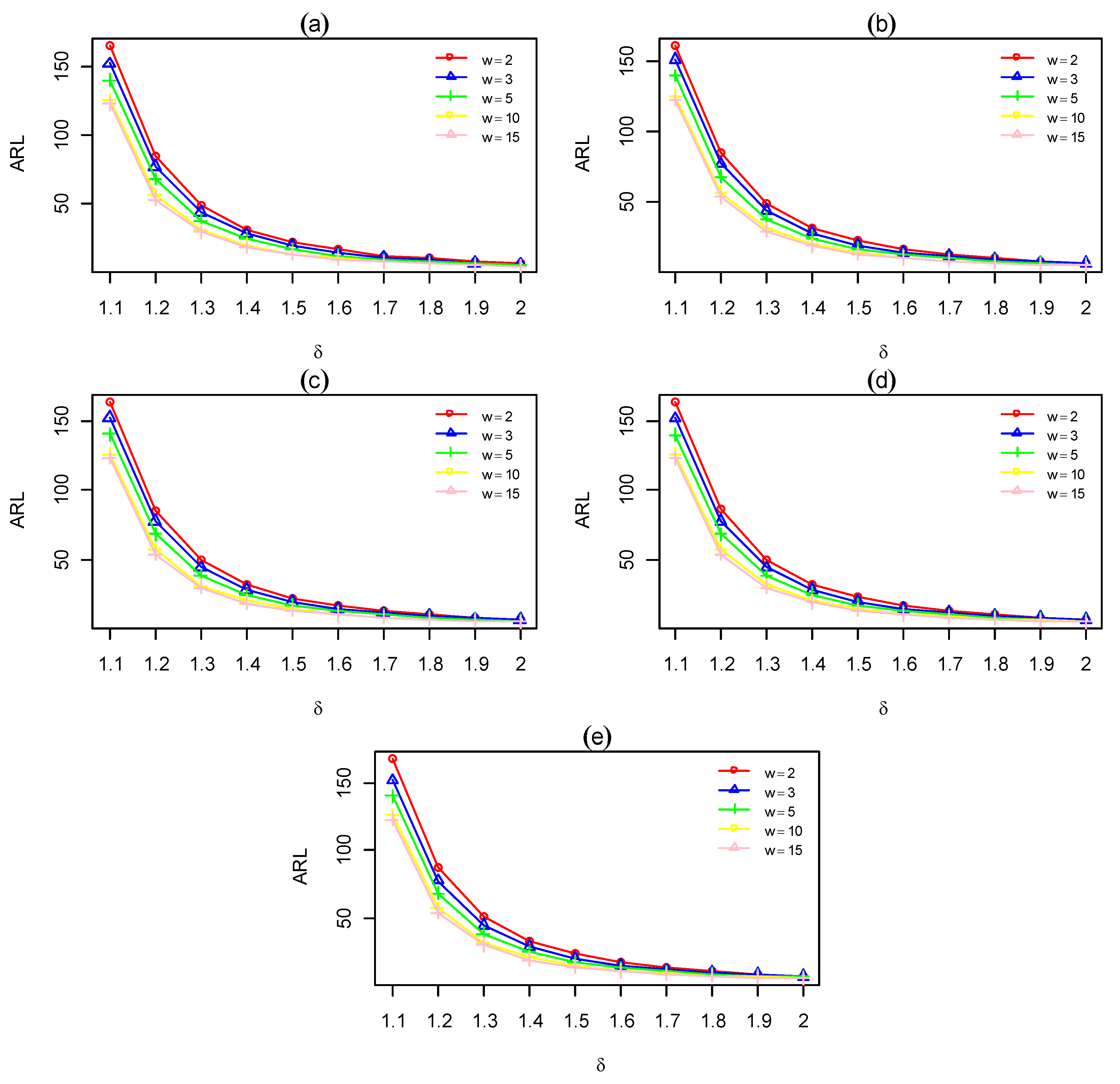
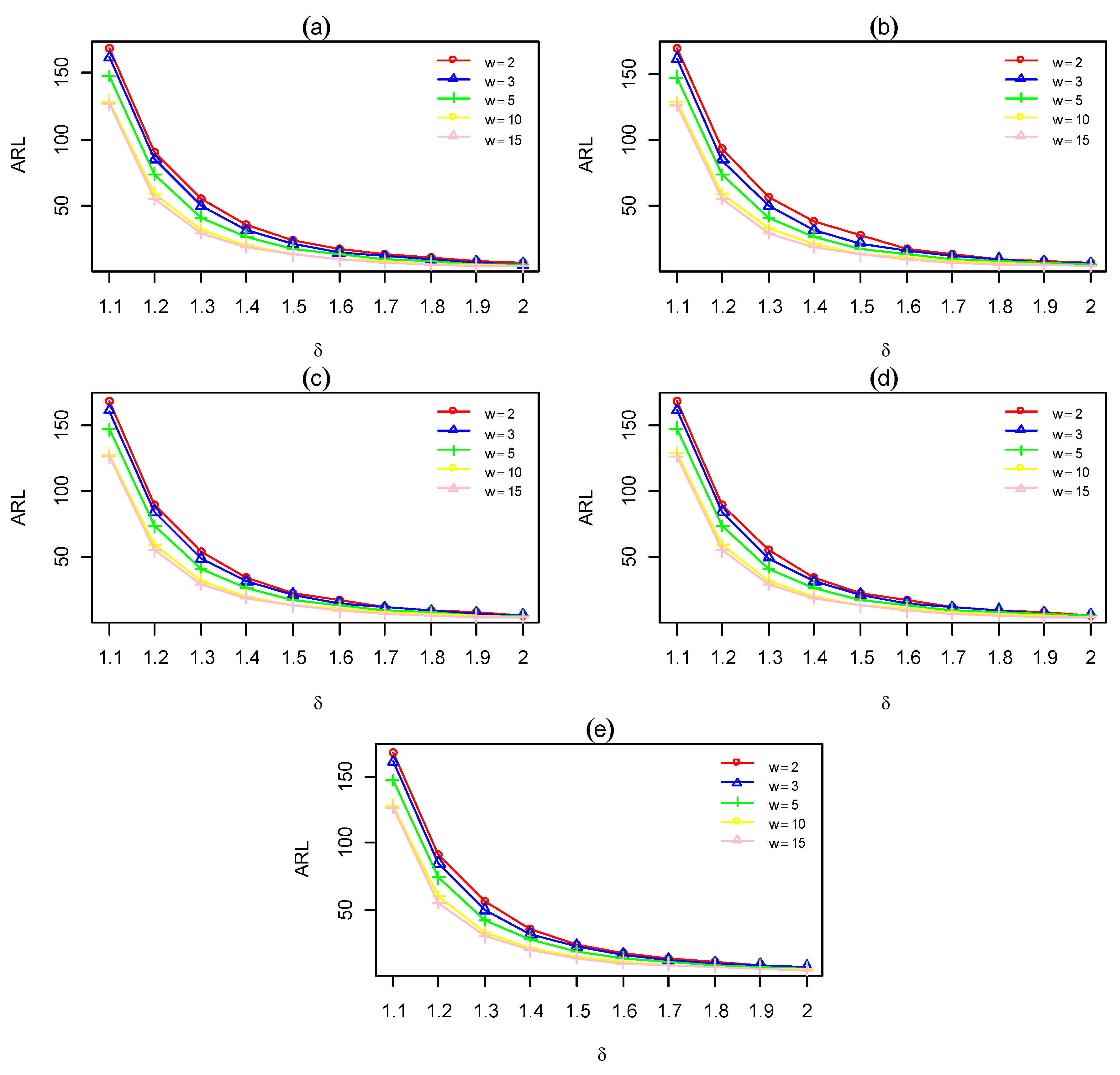
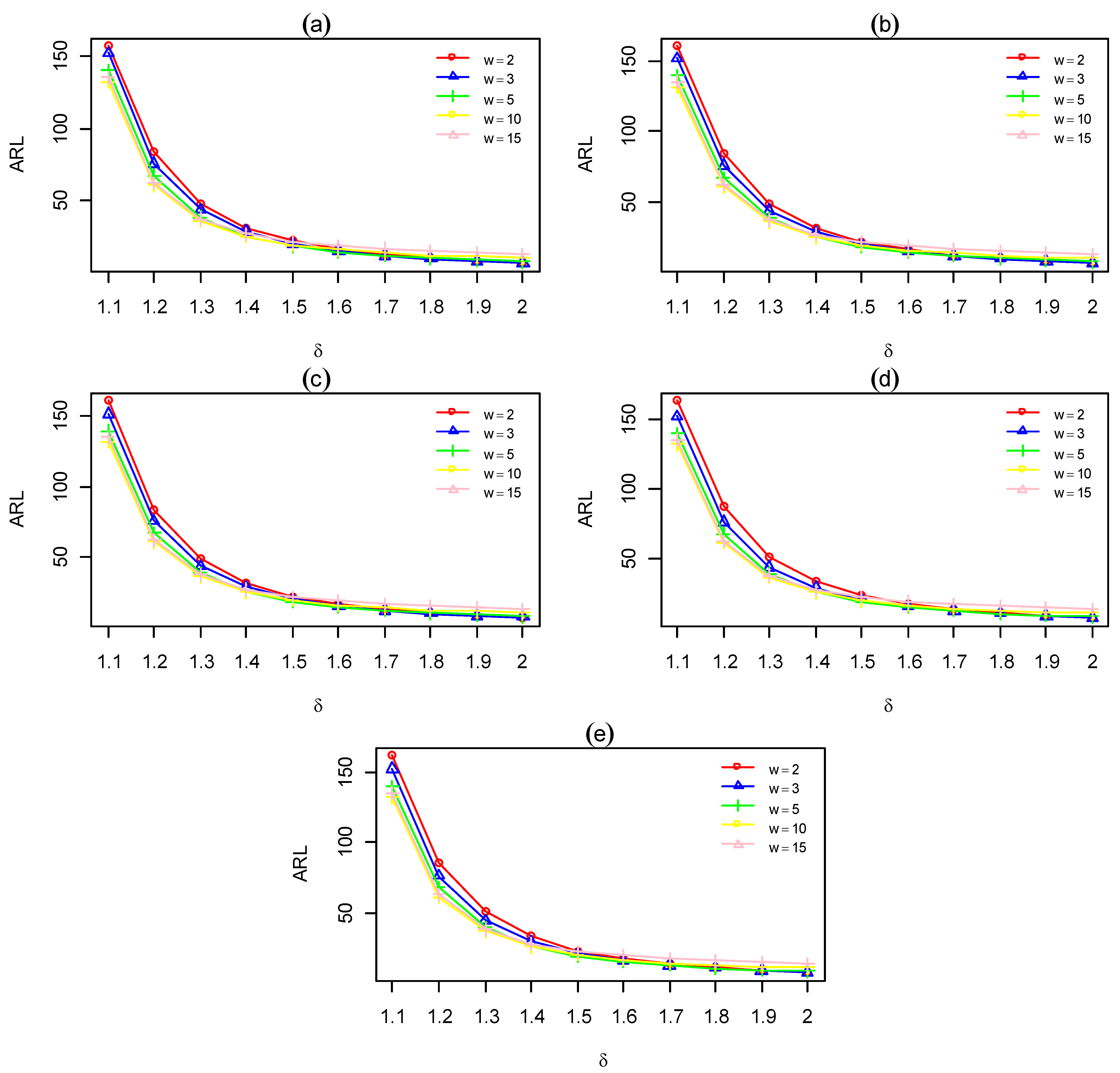
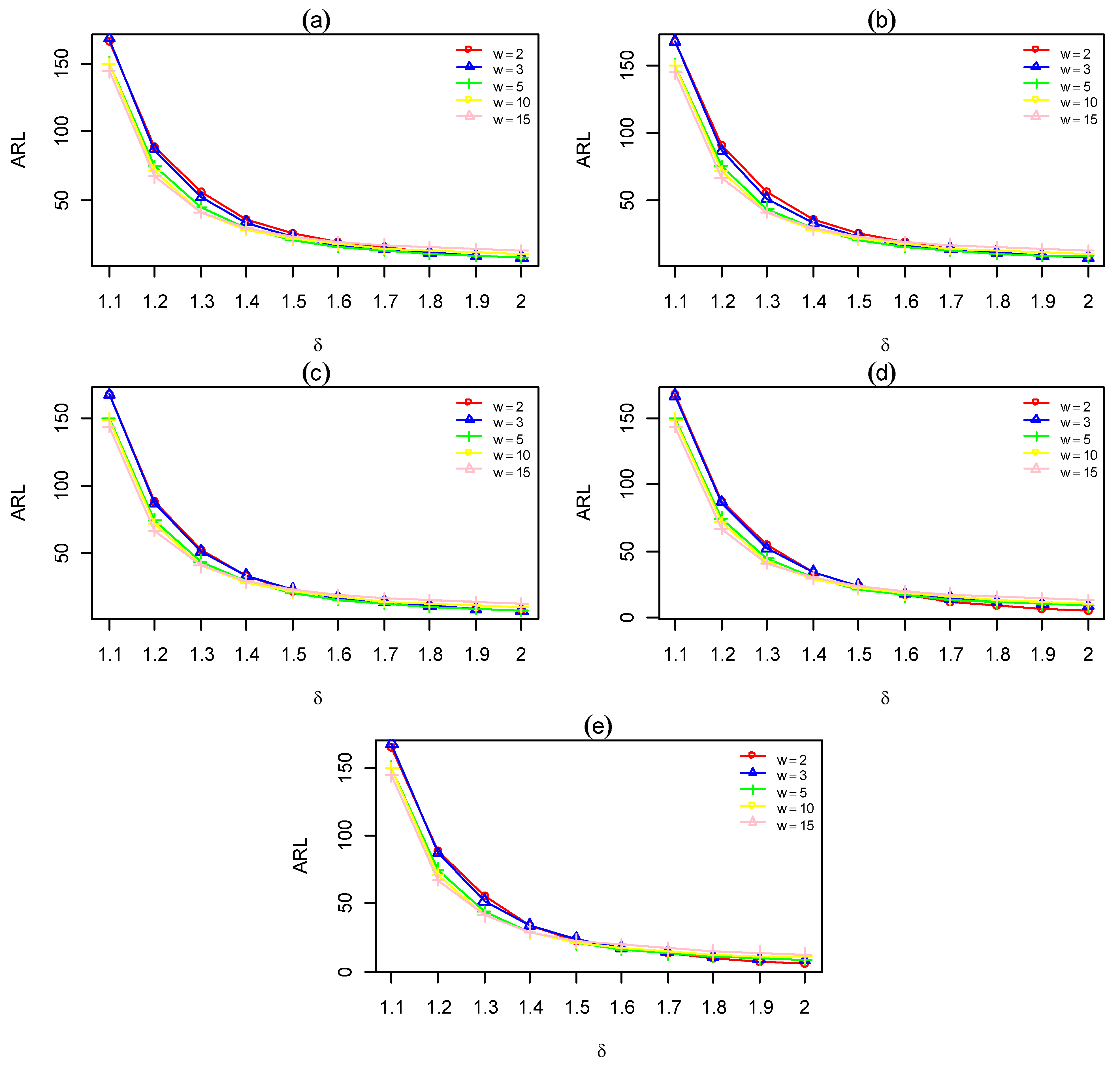
Furthermore, to check the effect of moving average span on the detection ability of the designed MA- and DMA- charts, sensitivity analysis was performed based on various choices of moving average span . The results of the sensitivity analysis for the MA- and DMA- charts with are presented in Figure 1, Figure 2, Figure 3 and Figure 4. At the pre-specified , it is noted that the performance ability of the MA- and DMA- charts increased with the increase in the moving average span. For example, it can be easily observed in Figure 1, Figure 2, Figure 3 and Figure 4 that at , both the designed charts have the lowest curves of for all the above-mentioned MSS schemes as compared to all the choices of for .
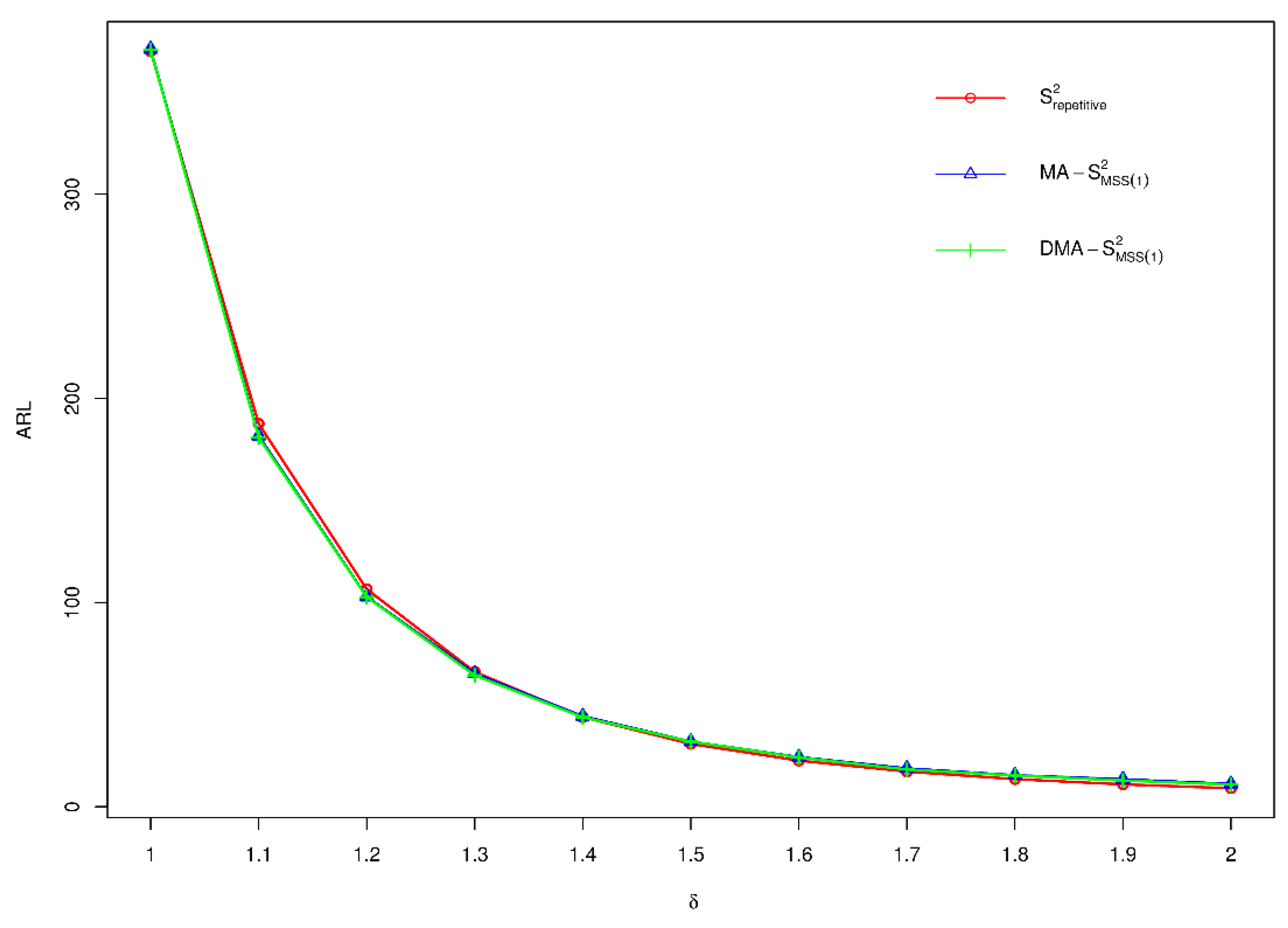
Furthermore, a comparative study of the best proposed MA- and DMA- charts with the existing chart was designed based on the repetitive sampling proposed by Aslam et al. [46]. For the pre-fixed and , the run length curves of the MA-, DMA- and are plotted in Figure 5. It is observed that for small amounts of shift (i.e., 1.1 to 1.5), the MA- and DMA- charts have comparatively better detection ability, while for large shifts (i.e., more than 1.5), the chart showed relatively lower ARL values. The dominance of the chart in the presence of large shifts is natural because of the Shewhart structure.
5. Case Study
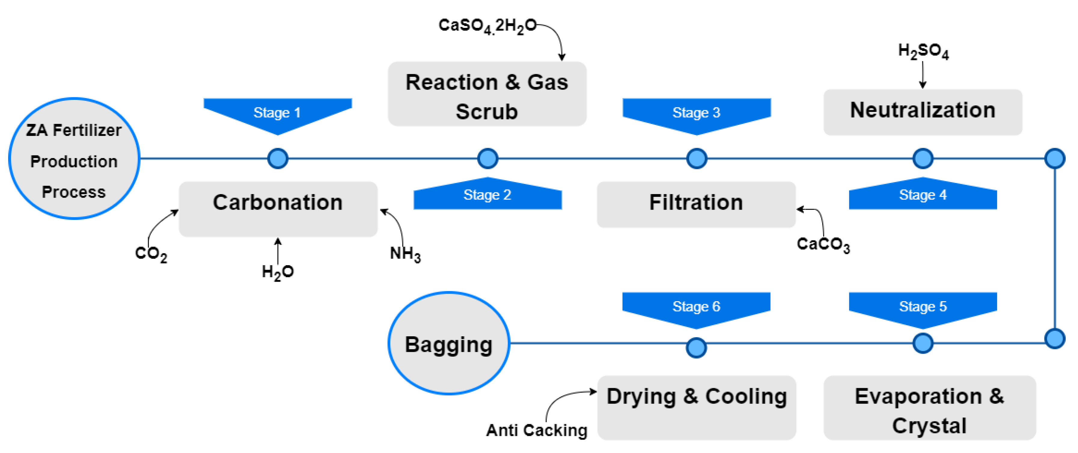
This section contains real-life applications of the designed control charts to monitor process dispersion in a ZA fertilizer production-based dataset. Mashuri et al. [47] also used this dataset to illustrate the better performance of proposed multivariate control charts in terms of monitoring the process variability. ZA fertilizer is frequently used to increase the concentration of sulfur and nitrogen in soil. It is also called ammonium sulfate fertilizer. The production process of ZA fertilizer is based on six stages (cf. Figure 6): carbonation, reaction and gas scrub, filtration, neutralization, evaporation and crystal, and drying and cooling stages. Air and carbon dioxide are emitted in this production process.
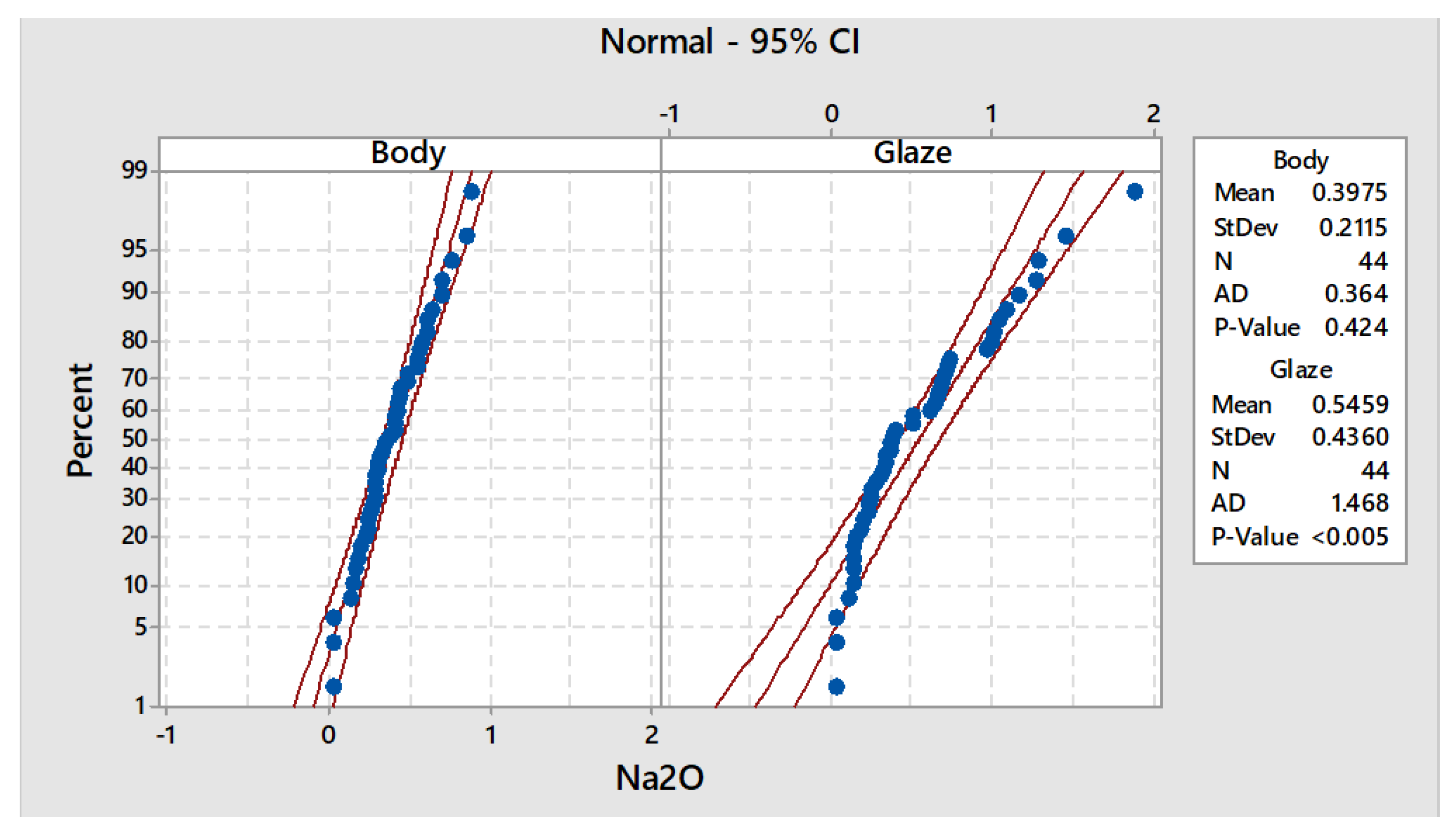
In this case study, the concentration of is the variable of interest in the fertilizer production process. This variable has 526 values consisting of the concentration of in the body and in the glassy coating on ceramics called glaze. These observations related to the body are considered in-control (239 values) data, while observations related to glaze are considered out-of-control (287 values) data. To assess the normality of both datasets, probability plots were prepared, which are shown in Figure 7. It should be noted that the in-control data are normally distributed, with a mean of 0.3975 and 0.2115 standard deviation. However, the out-of-control data are not normally distributed; their mean is 0.5459 with 0.424 standard deviation. By adopting the mechanism of MSS, 174 samples of size 5 were drawn from this dataset, which has two subgroups (79 in control and 95 out of control). To evaluate the performance of both the designed charts, the in-control subgroup of this dataset was utilized to calculate the proposed MA- and DMA- charts’ control limits at the pre-defined .
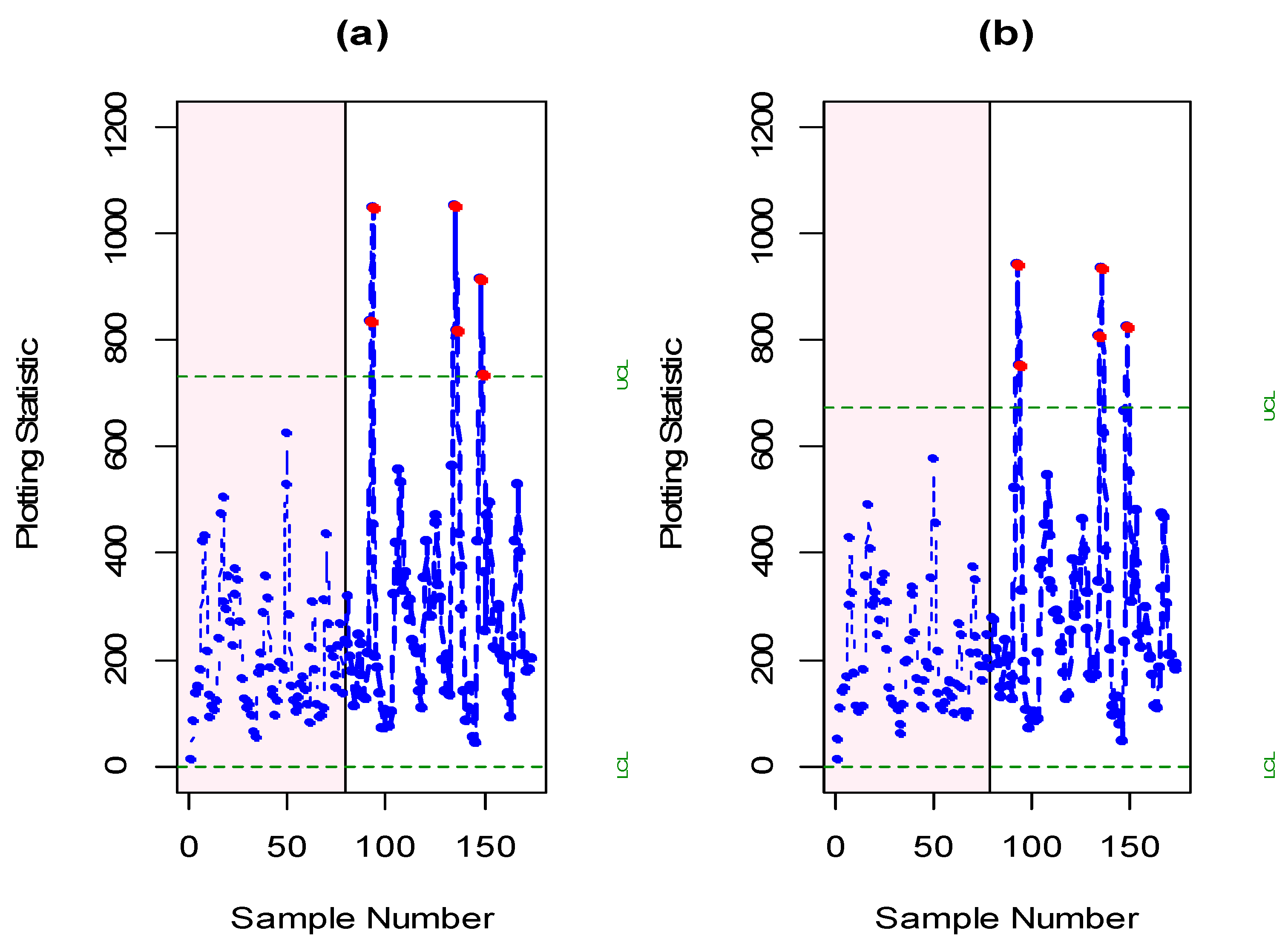
Figure 8 presents a graphical view of both the proposed charts. On the X-axis, the subgroups (sample numbers) are plotted, and on the y-axis, the plotting statistics of both the proposed charts are plotted against their respective control limits. The pink shaded area represents in-control points while white colored is referring to the out-of-control region. It shows that the MA- control chart detects an out-of-control signal after inspecting 92 samples, while the DMA- control chart detects out-of-control points after observing 90 samples. Both control charts have alternatively in-control and out-of-control points in out-of-control regions; therefore, a specific pattern can be seen in both the MA- and DMA- charts (cf. Figure 8). From the above simulation study, it is noted that the DMA- chart has outperformed the Shewhart- and MA- charts with a fixed amount of shift in the dispersion parameter. Similarly, by implementing the real-life example, we observe that the detection ability of the DMA- control chart is high, and it is more sensitive than the MA- control chart for the monitoring of process variability.
Furthermore, the proposed charts have wide real-life applications in different major fields of life. For example, we can utilize this control charting structure in the chemical industry, medical industry, glass field, ceramic industry, engineering, fertilizer production, hard-bake process and wind farm data (cf. Riaz et al. [22], Anwar et al. [24] and Khan et al. [29]).
6. Conclusions
Usually, memory-type control charts are used to detect small to moderate shifts in the location or dispersion process parameters. The process is said to be OOC depending on the amount of shift detected in the location or dispersion parameters. Usually, it is preferable to detect a shift in the dispersion parameter of the process before the detection of a shift in the location parameter. In this study, we have designed memory-type MA- and DMA- control charts for the monitoring of the process dispersion parameter using a modified successive sampling technique. Additionally, a comparative analysis with the existing Shewhart- chart has been presented using different performance measures (ARL, MDRL and SDRL). From the results, we have observed that the value of decreases with the increasing value of dispersion shift and sample size at a fixed value of (cf. Table 2 and Table 3). Moreover, the findings lead to the conclusion that the designed DMA- control chart performs better than Shewhart- and MA- under all the aforementioned MSS schemes. We have also noted that increasing values of the moving average span show a declining trend in curves under all MSS schemes (cf. Figure 1, Figure 2, Figure 3 and Figure 4).
Generally, the structure of mixed EWMA and CUSUM charts are more efficient compared to traditional MA, DMA, EWMA and CUSUM charts because they are more sensitive to the detection of small shifts in any process (cf. [48]). Therefore, one could extend this study by using different choices of MSS schemes and sample sizes to design a new mixed structure of the EWMA and CUSUM control charts. Moreover, the current study is designed based on the known parameter case (K-case), while the unknown parameter case (U-case) is recommended for future study. Furthermore, the MSS structure is proposed under normal distribution (symmetric distribution); however, one could propose MSS structure based on asymmetrical distribution and further extend the performance ability of the proposed control charts under the new MSS structure based on asymmetrical distributions.
Author Contributions
Conceptualization, M.H. and T.M.; methodology, M.H., T.M. and S.M.M.R.; software, M.H. and T.M.; validation, M.H., S.M.M.R., T.M. and N.A.; formal analysis, M.H.; writing—original draft preparation, M.H., N.A., T.M. and S.M.M.R.; writing—review and editing, M.H., N.A., T.M. and S.M.M.R.; visualization, M.H.; supervision, T.M. and S.M.M.R.; funding acquisition, T.M. All authors have read and agreed to the published version of the manuscript.
Funding
This publication is based on work supported by King Fahd University of Petroleum and Minerals. Tahir Mahmood and Nasir Abbas at KFUPM acknowledge the Interdisciplinary Research Center for Smart Mobility and Logistics for the support received under grant no. INML2205.
Data Availability Statement
Data sharing is not applicable to this article as no datasets were generated or analyzed during the current study.
Acknowledgments
We are thankful to King Fahd University of Petroleum and Minerals for providing us with research facilities for conducting this research.
Conflicts of Interest
The authors declare no conflict of interest.
References
- Arslan, M.; Anwar, S.; Gunaime, N.M.; Shahab, S.; Lone, S.A.; Rasheed, Z. An Improved Charting Scheme to Monitor the Process Mean Using Two Supplementary Variables. Symmetry 2023, 15, 482. [Google Scholar] [CrossRef]
- Shewhart, W.A. Quality control charts. Bell Syst. Tech. J. 1926, 5, 593–603. [Google Scholar] [CrossRef]
- Page, E.S. Continuous inspection schemes. Biometrika 1954, 41, 100–115. [Google Scholar] [CrossRef]
- Roberts, S. Control chart tests based on geometric moving averages. Technometrics 1959, 42, 97–101. [Google Scholar] [CrossRef]
- Wong, H.; Gan, F.; Chang, T. Designs of moving average control chart. J. Stat. Comput. Simul. 2004, 74, 47–62. [Google Scholar] [CrossRef]
- Alevizakos, V.; Chatterjee, K.; Koukouvinos, C.; Lappa, A. A double moving average control chart: Discussion. Commun. Stat.-Simul. Comput. 2020, 51, 6043–6057. [Google Scholar] [CrossRef]
- Hu, X.; Sun, G.; Xie, F.; Tang, A. Monitoring the Ratio of Two Normal Variables Based on Triple Exponentially Weighted Moving Average Control Charts with Fixed and Variable Sampling Intervals. Symmetry 2022, 14, 1236. [Google Scholar] [CrossRef]
- Khoo, M.B.; Yap, P. Joint monitoring of process mean and variability with a single moving average control chart. Qual. Eng. 2004, 17, 51–65. [Google Scholar] [CrossRef]
- Adeoti, O.A.; Akomolafe, A.A.; Adebola, F.B. Monitoring process variability using double moving average control chart. Ind. Eng. Manag. Syst. 2019, 18, 210–221. [Google Scholar] [CrossRef]
- Khoo, M.B.; Wong, V. A double moving average control chart. Commun. Stat.—Simul. Comput.® 2008, 37, 1696–1708. [Google Scholar] [CrossRef]
- Areepong, Y. Explicit formulas of average run length for a moving average control chart for monitoring the number of defective products. Int. J. Pure Appl. Math. 2012, 80, 331–343. [Google Scholar]
- Phant, S.; Sukparungsee, S.; Areepong, Y. Explicit formula for average run length of double moving control chart for INAR (1) processes. Preprint 2016. [Google Scholar] [CrossRef]
- Salazar, R.; Sinha, A. Control chart X based on ranked set sampling. Comun. Tecica 1997, 1, 1–97. [Google Scholar]
- Al-Nasser, A.D.; Al-Rawwash, M. A control chart based on ranked data. J. Appl. Sci. 2007, 7, 1936–1941. [Google Scholar]
- Abujiya, M.a.R.; Lee, M.H.; Riaz, M. Improving the performance of exponentially weighted moving average control charts. Qual. Reliab. Eng. Int. 2014, 30, 571–590. [Google Scholar] [CrossRef]
- Munir, W.; Haq, A. New cumulative sum control charts for monitoring process variability. J. Stat. Comput. Simul. 2017, 87, 2882–2899. [Google Scholar] [CrossRef]
- Nawaz, T.; Raza, M.A.; Han, D. A new approach to design efficient univariate control charts to monitor the process mean. Qual. Reliab. Eng. Int. 2018, 34, 1732–1751. [Google Scholar] [CrossRef]
- Nawaz, T.; Han, D. Monitoring the process location by using new ranked set sampling-based memory control charts. Qual. Technol. Quant. Manag. 2020, 17, 255–284. [Google Scholar] [CrossRef]
- Hussain, S.; Mahmood, T.; Riaz, M.; Nazir, H.Z. A new approach to design median control charts for location monitoring. Commun. Stat.-Simul. Comput. 2022, 51, 3553–3577. [Google Scholar] [CrossRef]
- Reynolds, M.R., Jr.; Lou, J. An evaluation of a GLR control chart for monitoring the process mean. J. Qual. Technol. 2010, 42, 287–310. [Google Scholar] [CrossRef]
- Sheriff, M.Z.; Karim, M.N.; Nounou, H.N.; Nounou, M.N. Process monitoring using PCA-based GLR methods: A comparative study. J. Comput. Sci. 2018, 27, 227–246. [Google Scholar] [CrossRef]
- Riaz, M.; Abbasi, S.A.; Abid, M.; Hamzat, A.K. A new HWMA dispersion control chart with an application to wind farm data. Mathematics 2020, 8, 2136. [Google Scholar] [CrossRef]
- Anwar, S.M.; Aslam, M.; Riaz, M.; Zaman, B. On mixed memory control charts based on auxiliary information for efficient process monitoring. Qual. Reliab. Eng. Int. 2020, 36, 1949–1968. [Google Scholar] [CrossRef]
- Anwar, S.M.; Aslam, M.; Zaman, B.; Riaz, M. Mixed memory control chart based on auxiliary information for simultaneously monitoring of process parameters: An application in glass field. Comput. Ind. Eng. 2021, 156, 107284. [Google Scholar] [CrossRef]
- Alevizakos, V.; Chatterjee, K.; Koukouvinos, C.; Lappa, A. A double generally weighted moving average control chart for monitoring the process variability. J. Appl. Stat. 2023. [Google Scholar] [CrossRef]
- Akhtar, N.; Abid, M.; Amir, M.W.; Abbas, Z.; Nazir, H.Z.; Raza, Z.; Riaz, M. Design and analysis of exponentially weighted moving average control charts for monitoring the variability of log-normal processes with estimated parameters. Qual. Reliab. Eng. Int. 2022, 38, 1590–1611. [Google Scholar] [CrossRef]
- Chatterjee, K.; Koukouvinos, C.; Lappa, A.; Roupa, P. A joint monitoring of the process mean and variance with a generally weighted moving average maximum control chart. Commun. Stat.-Simul. Comput. 2023. [Google Scholar] [CrossRef]
- Chatterjee, K.; Koukouvinos, C.; Lappa, A. Monitoring process mean and dispersion with one double generally weighted moving average control chart. J. Appl. Stat. 2023, 50, 19–42. [Google Scholar] [CrossRef]
- Khan, I.; Khan, D.M.; Noor-ul-Amin, M.; Khalil, U.; Alshanbari, H.M.; Ahmad, Z. Hybrid EWMA Control Chart under Bayesian Approach Using Ranked Set Sampling Schemes with Applications to Hard-Bake Process. Appl. Sci. 2023, 13, 2837. [Google Scholar] [CrossRef]
- Ajibade, G.A.; Ajadi, J.O.; Kuboye, O.J.; Alih, E. Generalized new exponentially weighted moving average control charts (NEWMA) for monitoring process dispersion. Int. J. Qual. Reliab. Manag. 2023. [Google Scholar] [CrossRef]
- Haq, A.; Abbasi, A.A. New weighted adaptive CUSUM charts for monitoring the generalized variance of a bivariate normal process. J. Stat. Comput. Simul. 2023, 93, 604–633. [Google Scholar] [CrossRef]
- Yaqub, M.; Abbas, N.; Riaz, M.; Shabbir, J. On modified successive sampling based control charting schemes. Qual. Reliab. Eng. Int. 2016, 32, 2491–2497. [Google Scholar] [CrossRef]
- Abbas, N.; Riaz, M.; Mahmood, T. An improved S2 control chart for cost and efficiency optimization. IEEE Access 2017, 5, 19486–19493. [Google Scholar] [CrossRef]
- Hyder, M.; Mahmood, T.; Butt, M.M.; Raza, S.M.M.; Abbas, N. On the location-based memory type control charts under modified successive sampling scheme. Qual. Reliab. Eng. Int. 2021, 38, 2200–2217. [Google Scholar] [CrossRef]
- Jessen, R.J. Statistical Investigation of a Sample Survey for Obtaining Farm Facts; Jessen, R.J., Ed.; Lowa State University: Ames, IA, USA, 1942. [Google Scholar]
- Patterson, H. Sampling on successive occasions with partial replacement of units. J. R. Stat. Society. Ser. B. 1950, 12, 241–255. [Google Scholar] [CrossRef]
- Rao, J.; Graham, J.E. Rotation designs for sampling on repeated occasions. J. Am. Stat. Assoc. 1964, 59, 492–509. [Google Scholar] [CrossRef]
- Choudhary, R.; Bathla, H.; Sud, U. On non-response in sampling on two occasions. J. Indian Soc. Agric. Stat. 2004, 58, 331–343. [Google Scholar]
- Jones, L.A.; Champ, C.W.; Rigdon, S.E. The performance of exponentially weighted moving average charts with estimated parameters. Technometrics 2001, 43, 156–167. [Google Scholar] [CrossRef]
- Noorossana, R.; Fathizadan, S.; Nayebpour, M.R. EWMA control chart performance with estimated parameters under non-normality. Qual. Reliab. Eng. Int. 2016, 32, 1637–1654. [Google Scholar] [CrossRef]
- Mahmood, T.; Erem, A. A bivariate exponentially weighted moving average control chart based on exceedance statistics. Comput. Ind. Eng. 2023, 175, 108910. [Google Scholar] [CrossRef]
- Omar, M.H.; Arafat, S.Y.; Hossain, M.P.; Riaz, M. Inverse Maxwell Distribution and Statistical Process Control: An Efficient Approach for Monitoring Positively Skewed Process. Symmetry 2021, 13, 189. [Google Scholar] [CrossRef]
- Erem, A.; Mahmood, T. A bivariate CUSUM control chart based on exceedance statistics. Qual. Reliab. Eng. Int. 2023, 39, 1172–1191. [Google Scholar] [CrossRef]
- Iqbal, A.; Mahmood, T.; Ali, Z.; Riaz, M. On Enhanced GLM-Based Monitoring: An Application to Additive Manufacturing Process. Symmetry 2022, 14, 122. [Google Scholar] [CrossRef]
- Berardinelli, C. Short-Run Statistical Process Control Techniques. Available online: https://www.isixsigma.com/control-charts/short-run-statistical-process-control-techniques/ (accessed on 6 April 2023).
- Aslam, M.; Khan, N.; Jun, C.-H. A new S2 control chart using repetitive sampling. J. Appl. Stat. 2015, 42, 2485–2496. [Google Scholar] [CrossRef]
- Mashuri, M.; Haryono, H.; Aksioma, D.F.; Wibawati, W.; Ahsan, M.; Khusna, H. Tr (R2) control charts based on kernel density estimation for monitoring multivariate variability process. Cogent Eng. 2019, 6, 1665949. [Google Scholar] [CrossRef]
- Zaman, B.; Abbas, N.; Riaz, M.; Lee, M.H. Mixed CUSUM-EWMA chart for monitoring process dispersion. Int. J. Adv. Manuf. Technol. 2016, 86, 3025–3039. [Google Scholar] [CrossRef]
Figure 1.
The effect of moving average span parameter (w) on the performance of the MA- control chart under MSS schemes for constant c = 2; (a) , (b) , (c) , (d) MSS(4), (e) .
Figure 1.
The effect of moving average span parameter (w) on the performance of the MA- control chart under MSS schemes for constant c = 2; (a) , (b) , (c) , (d) MSS(4), (e) .

Figure 2.
The effect of moving average span parameter (w) on the performance of the MA- control chart under MSS schemes for constant c = 3; (a) , (b) , (c) , (d) , (e) .
Figure 2.
The effect of moving average span parameter (w) on the performance of the MA- control chart under MSS schemes for constant c = 3; (a) , (b) , (c) , (d) , (e) .

Figure 3.
The effect of moving average span parameter (w) on the performance of the DMA- control chart under MSS schemes for constant c = 2; (a) , (b) , (c) , (d) , (e) .
Figure 3.
The effect of moving average span parameter (w) on the performance of the DMA- control chart under MSS schemes for constant c = 2; (a) , (b) , (c) , (d) , (e) .

Figure 4.
The influence of moving average span parameter (w) on the performance of the DMA- control chart under MSS schemes for constant c = 3; (a) , (b) , (c) , (d) , (e) .
Figure 4.
The influence of moving average span parameter (w) on the performance of the DMA- control chart under MSS schemes for constant c = 3; (a) , (b) , (c) , (d) , (e) .

Figure 5.
At a fixed constant , a comparison of the best proposed MA- and DMA- charts with the chart based on repetitive sampling .
Figure 5.
At a fixed constant , a comparison of the best proposed MA- and DMA- charts with the chart based on repetitive sampling .

Figure 6.
Stages of ZA fertilizer production process.

Figure 7.
The probability plots of the concentration of with respect to body and glaze.

Figure 8.
Demonstration for (a) MA- and (b) DMA- control charts using ZA fertilizer production dataset.
Figure 8.
Demonstration for (a) MA- and (b) DMA- control charts using ZA fertilizer production dataset.


Table 1.
Control charting coefficients and for the proposed control charts under different schemes of MSS (w = 2).
Table 1.
Control charting coefficients and for the proposed control charts under different schemes of MSS (w = 2).
| Scheme | ||||||||
|---|---|---|---|---|---|---|---|---|
| 1.08 | 0.37 | 10.18 | 17.14 | 0.97 | 0.26 | 10.72 | 17.74 | |
| 0.86 | 0.34 | 9.39 | 15.64 | 0.86 | 0.26 | 9.994 | 16.48 | |
| 0.73 | 0.38 | 8.37 | 13.84 | 0.8 | 0.28 | 9.36 | 15.35 | |
| 0.67 | 0.40 | 7.76 | 12.8 | 0.76 | 0.29 | 8.95 | 14.58 | |
| 0.64 | 0.42 | 7.49 | 12.3 | 0.74 | 0.30 | 8.78 | 14.27 | |
| 0.76 | 0.3 | 9.6 | 16.1 | 0.78 | 0.25 | 9.8 | 16.32 | |
| 0.55 | 0.40 | 7.12 | 11.85 | 0.68 | 0.29 | 8.5 | 14.04 | |
| 0.46 | 0.48 | 6.08 | 10.03 | 0.63 | 0.32 | 7.81 | 12.8 | |
| 0.43 | 0.51 | 5.75 | 9.53 | 0.60 | 0.34 | 7.5 | 12.23 | |
| 0.41 | 0.52 | 5.57 | 9.17 | 0.59 | 0.35 | 7.38 | 12.02 | |
Table 2.
Run length profile of the proposed charts under MSS at pre-specified and .
| Schemes | |||||||||||||||||||
|---|---|---|---|---|---|---|---|---|---|---|---|---|---|---|---|---|---|---|---|
| ARL | MDRL | SDRL | ARL | MDRL | SDRL | ARL | MDRL | SDRL | ARL | MDRL | SDRL | ARL | MDRL | SDRL | ARL | MDRL | SDRL | ||
| 1 | 369.56 | 309.5 | 369.08 | 369.21 | 308.1 | 371.56 | 371.03 | 254.00 | 375.92 | 369.91 | 260.00 | 368.71 | 370.61 | 261.00 | 367.68 | 369.37 | 251.00 | 363.10 | |
| 1.1 | 193.53 | 162 | 194.28 | 177.70 | 149 | 177.88 | 181.63 | 126.00 | 180.77 | 165.03 | 113.00 | 165.99 | 180.83 | 129.00 | 184.70 | 156.43 | 108.00 | 156.00 | |
| 1.2 | 113.28 | 94.5 | 113.41 | 97.62 | 82 | 97.61 | 102.83 | 72.00 | 102.67 | 85.11 | 59.00 | 85.59 | 102.64 | 73.00 | 98.51 | 83.57 | 58.00 | 82.99 | |
| 1.3 | 72.18 | 60.5 | 72.09 | 59.70 | 50 | 60.09 | 65.18 | 44.00 | 62.99 | 49.36 | 34.00 | 49.42 | 64.29 | 46.00 | 64.25 | 47.61 | 34.00 | 45.74 | |
| 1.4 | 49.45 | 41.5 | 49.48 | 39.16 | 32.5 | 39.31 | 44.30 | 30.00 | 42.58 | 31.72 | 22.00 | 29.82 | 43.79 | 31.00 | 44.25 | 31.67 | 22.00 | 31.76 | |
| 1.5 | 35.53 | 29.5 | 35.46 | 27.24 | 23 | 27.26 | 31.87 | 23.00 | 30.27 | 22.35 | 16.00 | 20.70 | 31.83 | 22.00 | 31.50 | 22.27 | 15.00 | 22.18 | |
| 1.6 | 26.97 | 22.5 | 26.90 | 20.18 | 17 | 20.37 | 24.27 | 17.00 | 22.70 | 16.58 | 12.00 | 14.84 | 24.09 | 17.00 | 23.82 | 16.38 | 11.00 | 16.44 | |
| 1.7 | 21.23 | 17.5 | 21.13 | 15.36 | 12.5 | 15.33 | 18.73 | 14.00 | 17.74 | 12.88 | 9.00 | 11.46 | 18.20 | 13.00 | 18.10 | 12.54 | 9.00 | 12.25 | |
| 1.8 | 17.04 | 14.5 | 16.96 | 12.23 | 10 | 12.15 | 15.38 | 11.00 | 13.95 | 10.58 | 8.00 | 9.13 | 15.25 | 11.00 | 14.78 | 10.18 | 7.00 | 9.93 | |
| 1.9 | 14.09 | 11.5 | 14.00 | 9.94 | 8.5 | 9.81 | 13.39 | 10.00 | 11.94 | 8.95 | 7.00 | 7.54 | 12.83 | 9.00 | 12.16 | 8.09 | 6.00 | 7.83 | |
| 2 | 11.88 | 9.5 | 11.78 | 8.32 | 6.5 | 8.22 | 11.15 | 8.00 | 9.96 | 7.55 | 6.00 | 6.13 | 10.84 | 8.00 | 10.20 | 7.10 | 5.00 | 6.79 | |
| 1 | 370.31 | 310 | 371.98 | 370.72 | 310.1 | 375.07 | 369.67 | 249.00 | 368.53 | 369.49 | 252.00 | 369.52 | 369.95 | 250.00 | 373.62 | 369.56 | 253.00 | 357.75 | |
| 1.1 | 200.19 | 167 | 202.15 | 183.68 | 153.5 | 185.50 | 181.62 | 124.00 | 185.11 | 161.31 | 111.00 | 163.25 | 180.49 | 127.00 | 186.63 | 160.13 | 113.00 | 159.44 | |
| 1.2 | 119.88 | 99.5 | 121.58 | 102.47 | 86 | 103.13 | 102.96 | 71.00 | 104.10 | 85.62 | 59.00 | 86.67 | 101.68 | 72.00 | 103.17 | 84.08 | 59.00 | 84.42 | |
| 1.3 | 77.33 | 64.5 | 78.68 | 62.62 | 52 | 63.46 | 66.06 | 45.00 | 67.80 | 49.21 | 34.00 | 49.95 | 64.60 | 45.00 | 63.28 | 48.95 | 35.00 | 47.53 | |
| 1.4 | 53.30 | 44 | 54.19 | 41.59 | 34.5 | 42.56 | 44.46 | 31.00 | 43.19 | 32.37 | 23.00 | 31.23 | 44.38 | 30.00 | 46.02 | 31.60 | 22.00 | 31.74 | |
| 1.5 | 38.63 | 32 | 39.71 | 29.24 | 24.5 | 29.94 | 32.26 | 23.00 | 31.26 | 22.38 | 16.00 | 21.27 | 31.76 | 22.00 | 32.73 | 22.12 | 15.00 | 22.46 | |
| 1.6 | 29.29 | 24.5 | 30.11 | 21.33 | 18 | 21.85 | 24.60 | 18.00 | 23.25 | 16.70 | 12.00 | 15.49 | 23.95 | 17.00 | 24.32 | 16.13 | 11.00 | 16.35 | |
| 1.7 | 22.69 | 19 | 23.32 | 16.33 | 13.5 | 16.61 | 19.64 | 14.00 | 18.83 | 12.85 | 9.00 | 11.50 | 18.27 | 13.00 | 18.75 | 12.44 | 9.00 | 12.73 | |
| 1.8 | 18.49 | 15.5 | 19.18 | 12.93 | 10.5 | 13.27 | 15.53 | 11.00 | 14.27 | 10.53 | 8.00 | 9.26 | 15.16 | 10.00 | 15.78 | 9.66 | 7.00 | 9.74 | |
| 1.9 | 15.15 | 12.5 | 15.69 | 10.51 | 9 | 10.77 | 13.14 | 9.00 | 12.18 | 8.88 | 6.00 | 7.70 | 12.55 | 8.00 | 12.94 | 8.06 | 5.00 | 8.22 | |
| 2 | 12.70 | 10.5 | 13.19 | 8.65 | 7 | 8.82 | 11.32 | 8.00 | 10.23 | 7.54 | 5.00 | 6.28 | 10.47 | 7.00 | 10.66 | 6.55 | 4.00 | 6.56 | |
| 1 | 370.12 | 313.5 | 375.77 | 369.67 | 306.5 | 367.15 | 370.35 | 250.50 | 375.53 | 369.46 | 256.00 | 372.18 | 370.45 | 261.00 | 372.14 | 369.14 | 260.00 | 367.74 | |
| 1.1 | 206.36 | 172.5 | 208.55 | 184.49 | 154 | 185.84 | 186.20 | 128.00 | 189.26 | 163.16 | 113.00 | 167.37 | 184.92 | 134.00 | 193.63 | 160.93 | 112.00 | 157.70 | |
| 1.2 | 124.14 | 103.5 | 126.43 | 103.32 | 86 | 105.21 | 105.86 | 73.00 | 108.69 | 85.53 | 59.00 | 87.62 | 103.29 | 77.00 | 108.00 | 83.53 | 58.00 | 82.80 | |
| 1.3 | 81.44 | 68 | 83.01 | 63.94 | 53 | 65.25 | 66.60 | 44.00 | 70.46 | 49.61 | 33.00 | 51.83 | 65.23 | 48.00 | 70.38 | 49.32 | 35.00 | 47.16 | |
| 1.4 | 56.46 | 47 | 58.17 | 42.17 | 35 | 43.11 | 44.64 | 30.00 | 46.71 | 32.43 | 23.00 | 30.68 | 43.51 | 33.00 | 46.87 | 31.81 | 22.00 | 32.94 | |
| 1.5 | 41.10 | 34.5 | 42.65 | 29.71 | 25 | 30.59 | 33.15 | 23.00 | 32.21 | 22.66 | 16.00 | 21.75 | 32.08 | 21.00 | 34.05 | 21.93 | 15.00 | 23.10 | |
| 1.6 | 31.10 | 26 | 32.49 | 22.06 | 18.5 | 22.76 | 25.62 | 18.00 | 25.12 | 16.64 | 12.00 | 15.30 | 23.93 | 16.00 | 25.34 | 16.07 | 11.00 | 16.91 | |
| 1.7 | 24.32 | 20 | 25.58 | 16.70 | 13.5 | 17.38 | 19.83 | 14.00 | 19.00 | 13.15 | 9.00 | 11.84 | 18.70 | 12.00 | 19.91 | 12.31 | 8.00 | 13.00 | |
| 1.8 | 19.49 | 16 | 20.61 | 13.20 | 10.5 | 13.84 | 16.11 | 11.00 | 15.28 | 10.49 | 7.00 | 9.38 | 15.14 | 10.00 | 16.26 | 9.65 | 6.00 | 10.09 | |
| 1.9 | 16.00 | 13.5 | 16.99 | 10.63 | 9 | 11.12 | 13.35 | 9.00 | 12.44 | 8.90 | 6.00 | 7.72 | 12.40 | 8.00 | 13.48 | 7.84 | 5.00 | 8.28 | |
| 2 | 13.40 | 11 | 14.31 | 8.89 | 7 | 9.28 | 11.59 | 8.00 | 10.72 | 7.48 | 5.00 | 6.30 | 10.12 | 6.00 | 10.88 | 6.60 | 4.00 | 6.91 | |
| 1 | 370.03 | 313.5 | 379.63 | 370.33 | 313.5 | 378.75 | 369.81 | 252.50 | 371.42 | 369.00 | 256.00 | 369.53 | 370.51 | 254.00 | 376.92 | 370.17 | 257.00 | 374.43 | |
| 1.1 | 207.91 | 173.5 | 211.00 | 189.03 | 157.5 | 191.70 | 185.47 | 126.00 | 192.29 | 163.40 | 111.00 | 170.20 | 185.00 | 131.00 | 191.72 | 162.91 | 114.50 | 165.71 | |
| 1.2 | 127.41 | 106.5 | 129.93 | 107.02 | 89 | 108.71 | 105.98 | 72.00 | 109.41 | 86.78 | 60.00 | 86.12 | 105.25 | 77.00 | 110.24 | 86.10 | 59.00 | 89.59 | |
| 1.3 | 84.13 | 70 | 86.42 | 66.26 | 55 | 67.76 | 66.83 | 45.00 | 70.29 | 51.16 | 36.00 | 49.78 | 65.35 | 49.00 | 69.44 | 49.78 | 33.00 | 52.16 | |
| 1.4 | 58.41 | 48.5 | 60.58 | 44.02 | 36.5 | 45.16 | 45.14 | 33.00 | 45.75 | 33.18 | 24.00 | 31.32 | 44.46 | 30.00 | 47.31 | 31.71 | 21.00 | 33.36 | |
| 1.5 | 42.51 | 35.5 | 44.10 | 30.86 | 25.5 | 31.93 | 34.47 | 24.00 | 33.89 | 22.97 | 16.00 | 22.01 | 31.94 | 21.00 | 34.68 | 22.19 | 15.00 | 23.34 | |
| 1.6 | 32.41 | 26.5 | 34.13 | 22.66 | 19 | 23.57 | 26.15 | 18.00 | 25.75 | 16.89 | 12.00 | 15.81 | 23.72 | 16.00 | 25.68 | 16.07 | 11.00 | 16.88 | |
| 1.7 | 25.32 | 21 | 26.93 | 17.35 | 14 | 18.33 | 20.49 | 14.00 | 19.97 | 13.01 | 9.00 | 11.90 | 18.59 | 12.00 | 20.30 | 12.21 | 8.00 | 13.18 | |
| 1.8 | 20.21 | 16.5 | 21.49 | 13.68 | 11 | 14.42 | 16.48 | 12.00 | 15.65 | 10.79 | 8.00 | 9.86 | 14.92 | 10.00 | 16.31 | 9.65 | 6.00 | 10.29 | |
| 1.9 | 16.72 | 14 | 17.94 | 11.10 | 9.5 | 11.72 | 13.76 | 10.00 | 13.08 | 9.01 | 6.00 | 8.01 | 12.26 | 8.00 | 13.69 | 7.85 | 5.00 | 8.36 | |
| 2 | 14.02 | 11.5 | 15.26 | 9.09 | 7.5 | 9.62 | 11.62 | 8.00 | 11.10 | 7.54 | 5.00 | 6.39 | 10.21 | 6.00 | 11.23 | 6.44 | 4.00 | 6.84 | |
| 1 | 370.87 | 311.5 | 373.74 | 370.04 | 316 | 377.20 | 369.75 | 250.00 | 378.34 | 371.98 | 258.00 | 375.82 | 369.95 | 252.00 | 367.78 | 369.82 | 261.00 | 358.28 | |
| 1.1 | 208.89 | 174.5 | 211.68 | 188.64 | 157.5 | 190.19 | 187.49 | 129.00 | 192.44 | 167.65 | 115.00 | 172.97 | 186.50 | 129.00 | 188.01 | 161.28 | 111.00 | 162.45 | |
| 1.2 | 128.23 | 107 | 131.36 | 107.90 | 90 | 109.52 | 106.97 | 73.00 | 111.64 | 86.99 | 59.00 | 91.39 | 105.16 | 75.00 | 108.44 | 85.08 | 60.00 | 82.69 | |
| 1.3 | 85.32 | 71 | 88.56 | 66.78 | 55.5 | 68.19 | 67.23 | 45.00 | 71.09 | 50.54 | 35.00 | 48.99 | 66.90 | 48.00 | 67.66 | 50.12 | 34.00 | 51.97 | |
| 1.4 | 59.26 | 49 | 61.36 | 44.49 | 37 | 46.04 | 45.19 | 30.00 | 48.68 | 32.98 | 23.00 | 32.17 | 44.21 | 34.00 | 47.13 | 32.16 | 22.00 | 33.95 | |
| 1.5 | 43.07 | 35.5 | 45.14 | 31.10 | 26 | 32.17 | 32.15 | 21.00 | 35.36 | 21.91 | 16.00 | 21.82 | 31.59 | 24.00 | 34.09 | 21.64 | 15.00 | 23.81 | |
| 1.6 | 32.60 | 27 | 34.48 | 23.10 | 19 | 24.01 | 25.99 | 18.00 | 25.76 | 16.76 | 12.00 | 15.52 | 24.01 | 16.00 | 26.75 | 16.12 | 11.00 | 17.26 | |
| 1.7 | 25.61 | 21 | 27.48 | 17.55 | 14.5 | 18.42 | 20.53 | 14.00 | 19.85 | 13.25 | 9.00 | 12.26 | 18.60 | 12.00 | 20.60 | 12.39 | 8.00 | 13.36 | |
| 1.8 | 20.54 | 16.5 | 22.18 | 13.87 | 11 | 14.59 | 16.64 | 12.00 | 15.96 | 10.67 | 8.00 | 9.68 | 14.99 | 9.00 | 16.92 | 9.63 | 6.00 | 10.59 | |
| 1.9 | 16.79 | 13.5 | 18.27 | 11.22 | 9.5 | 11.90 | 13.81 | 10.00 | 13.34 | 8.91 | 6.00 | 7.96 | 12.27 | 8.00 | 13.72 | 7.95 | 5.00 | 8.55 | |
| 2 | 14.06 | 11.5 | 15.44 | 9.22 | 7.5 | 9.81 | 11.43 | 8.00 | 10.75 | 7.59 | 5.00 | 6.57 | 9.95 | 6.00 | 11.23 | 6.45 | 4.00 | 6.80 | |
Table 3.
Run length profile of the proposed charts under MSS at pre-specified and .
| Schemes | |||||||||||||||||||
|---|---|---|---|---|---|---|---|---|---|---|---|---|---|---|---|---|---|---|---|
| ARL | MDRL | SDRL | ARL | MDRL | SDRL | ARL | MDRL | SDRL | ARL | MDRL | SDRL | ARL | MDRL | SDRL | ARL | MDRL | SDRL | ||
| 1 | 370.83 | 311 | 379.94 | 370.13 | 313 | 377.80 | 370.40 | 257.00 | 371.47 | 369.86 | 250.00 | 370.83 | 370.31 | 254.00 | 375.76 | 370.99 | 256.00 | 368.59 | |
| 1.1 | 208.43 | 173 | 213.70 | 187.60 | 156 | 191.13 | 195.24 | 134.00 | 201.60 | 167.49 | 115.00 | 171.74 | 194.09 | 133.00 | 194.52 | 165.25 | 124.00 | 176.65 | |
| 1.2 | 126.35 | 105 | 130.14 | 106.39 | 89 | 108.87 | 116.99 | 79.00 | 123.07 | 88.44 | 66.00 | 91.71 | 115.63 | 80.00 | 115.91 | 90.60 | 61.00 | 93.61 | |
| 1.3 | 82.62 | 68.5 | 85.98 | 65.75 | 54.5 | 68.32 | 74.97 | 50.00 | 78.58 | 55.56 | 38.00 | 55.71 | 74.67 | 51.00 | 77.00 | 55.05 | 37.00 | 57.81 | |
| 1.4 | 58.02 | 47.5 | 61.31 | 43.29 | 36 | 45.25 | 50.99 | 34.00 | 54.33 | 35.96 | 25.00 | 35.37 | 50.68 | 36.00 | 52.94 | 35.75 | 24.00 | 38.52 | |
| 1.5 | 42.32 | 35 | 45.48 | 30.70 | 25 | 32.42 | 37.22 | 25.00 | 39.90 | 25.21 | 17.00 | 24.76 | 37.09 | 26.00 | 37.35 | 24.18 | 16.00 | 25.77 | |
| 1.6 | 31.92 | 26 | 34.57 | 22.47 | 18.5 | 23.80 | 28.77 | 19.00 | 29.37 | 18.82 | 13.00 | 18.38 | 27.72 | 20.00 | 28.62 | 17.92 | 12.00 | 19.15 | |
| 1.7 | 25.01 | 20 | 27.42 | 17.15 | 14 | 18.35 | 23.06 | 16.00 | 23.26 | 15.05 | 11.00 | 14.37 | 21.65 | 14.00 | 23.88 | 13.39 | 9.00 | 14.45 | |
| 1.8 | 20.22 | 16.5 | 22.22 | 13.51 | 11 | 14.64 | 18.50 | 12.00 | 18.86 | 11.70 | 8.00 | 11.15 | 17.29 | 11.00 | 19.08 | 10.78 | 7.00 | 11.59 | |
| 1.9 | 16.63 | 13.5 | 18.44 | 10.92 | 8.5 | 11.96 | 15.26 | 10.00 | 15.80 | 9.77 | 7.00 | 8.88 | 14.62 | 9.00 | 16.32 | 8.56 | 5.00 | 9.37 | |
| 2 | 13.88 | 11 | 15.63 | 9.09 | 7.5 | 9.88 | 13.09 | 9.00 | 13.18 | 8.19 | 6.00 | 7.41 | 12.29 | 8.00 | 13.81 | 7.19 | 4.00 | 7.65 | |
| 1 | 369.52 | 307 | 376.50 | 370.10 | 313 | 379.64 | 370.76 | 256.00 | 388.48 | 369.39 | 248.00 | 372.77 | 370.38 | 255.00 | 373.82 | 369.72 | 264.00 | 371.97 | |
| 1.1 | 211.02 | 175.5 | 219.56 | 190.71 | 158 | 195.74 | 198.16 | 135.00 | 211.65 | 168.35 | 111.00 | 172.04 | 197.03 | 135.00 | 203.24 | 167.05 | 121.00 | 166.65 | |
| 1.2 | 131.91 | 109 | 139.26 | 108.75 | 90 | 112.75 | 115.59 | 77.00 | 126.94 | 92.59 | 60.00 | 94.35 | 114.09 | 81.00 | 126.98 | 91.57 | 64.00 | 91.41 | |
| 1.3 | 87.46 | 71.5 | 93.80 | 68.32 | 56.5 | 71.99 | 74.23 | 47.00 | 83.80 | 57.30 | 36.00 | 57.04 | 73.85 | 52.00 | 78.44 | 55.97 | 39.00 | 56.26 | |
| 1.4 | 61.64 | 50 | 66.89 | 45.49 | 37.5 | 48.13 | 49.71 | 31.00 | 56.71 | 37.96 | 22.00 | 37.64 | 48.37 | 36.00 | 56.04 | 35.60 | 24.00 | 35.41 | |
| 1.5 | 45.13 | 36.5 | 50.20 | 32.17 | 26.5 | 34.72 | 36.58 | 22.00 | 42.17 | 27.32 | 14.00 | 26.18 | 35.98 | 25.00 | 39.90 | 25.11 | 17.00 | 25.47 | |
| 1.6 | 34.21 | 27.5 | 38.58 | 23.62 | 19 | 25.91 | 27.74 | 19.00 | 30.29 | 18.81 | 13.00 | 18.78 | 27.24 | 17.00 | 31.56 | 17.06 | 11.00 | 19.33 | |
| 1.7 | 26.68 | 21 | 30.66 | 17.98 | 14.5 | 19.77 | 22.53 | 14.00 | 24.42 | 14.34 | 10.00 | 14.14 | 20.63 | 12.00 | 24.96 | 13.13 | 8.00 | 14.82 | |
| 1.8 | 21.61 | 17 | 25.21 | 14.12 | 11 | 15.83 | 18.94 | 12.00 | 20.21 | 11.53 | 8.00 | 11.20 | 16.42 | 9.00 | 20.10 | 10.09 | 6.00 | 11.45 | |
| 1.9 | 17.65 | 13.5 | 20.85 | 11.36 | 9 | 12.81 | 15.40 | 10.00 | 16.45 | 9.55 | 6.00 | 9.05 | 13.72 | 7.00 | 17.05 | 8.30 | 5.00 | 9.44 | |
| 2 | 14.78 | 11.5 | 17.64 | 9.40 | 7 | 10.69 | 13.11 | 8.00 | 14.14 | 8.03 | 5.00 | 7.60 | 11.30 | 6.00 | 14.25 | 6.83 | 4.00 | 7.94 | |
| 1 | 370.11 | 311.5 | 385.43 | 369.13 | 306.5 | 372.65 | 369.21 | 251.00 | 383.21 | 369.71 | 248.00 | 381.95 | 370.38 | 260.00 | 376.17 | 370.92 | 255.00 | 378.80 | |
| 1.1 | 217.49 | 180.5 | 228.07 | 190.47 | 158 | 195.58 | 197.04 | 130.00 | 216.21 | 168.85 | 112.00 | 179.77 | 196.47 | 136.00 | 207.60 | 167.63 | 121.00 | 175.42 | |
| 1.2 | 135.84 | 111.5 | 145.65 | 110.47 | 92 | 114.50 | 116.06 | 75.00 | 131.40 | 89.47 | 59.00 | 95.15 | 115.87 | 81.00 | 125.95 | 88.79 | 65.00 | 92.54 | |
| 1.3 | 91.23 | 74 | 99.84 | 69.39 | 57 | 73.47 | 73.84 | 46.00 | 84.78 | 54.44 | 36.00 | 59.81 | 72.27 | 52.00 | 82.88 | 53.10 | 38.00 | 57.29 | |
| 1.4 | 64.46 | 52 | 71.81 | 46.38 | 38.5 | 49.53 | 48.80 | 29.00 | 58.16 | 34.79 | 22.00 | 39.39 | 47.11 | 35.00 | 58.31 | 33.72 | 25.00 | 37.26 | |
| 1.5 | 47.28 | 37.5 | 53.58 | 32.68 | 27 | 35.63 | 36.23 | 21.00 | 43.98 | 23.42 | 14.00 | 26.69 | 35.54 | 25.00 | 42.80 | 22.60 | 17.00 | 26.13 | |
| 1.6 | 35.71 | 28 | 41.39 | 24.33 | 19.5 | 26.87 | 26.55 | 15.00 | 32.32 | 17.91 | 13.00 | 18.98 | 25.73 | 19.00 | 32.82 | 17.21 | 10.00 | 19.93 | |
| 1.7 | 28.14 | 22 | 33.37 | 18.45 | 14.5 | 20.73 | 20.58 | 11.00 | 25.72 | 14.62 | 10.00 | 14.48 | 20.51 | 15.00 | 26.23 | 12.93 | 8.00 | 14.93 | |
| 1.8 | 22.69 | 17.5 | 27.22 | 14.44 | 11.5 | 16.40 | 17.89 | 12.00 | 20.89 | 11.69 | 8.00 | 11.62 | 16.15 | 8.00 | 21.03 | 10.15 | 6.00 | 11.98 | |
| 1.9 | 18.46 | 14 | 22.64 | 11.61 | 9 | 13.32 | 12.91 | 6.00 | 17.23 | 9.45 | 6.00 | 9.19 | 11.64 | 9.00 | 17.33 | 8.03 | 4.00 | 9.68 | |
| 2 | 15.32 | 11.5 | 19.01 | 9.58 | 7.5 | 11.14 | 11.12 | 5.00 | 14.65 | 8.10 | 5.00 | 7.57 | 10.00 | 8.00 | 14.52 | 6.64 | 4.00 | 7.90 | |
| 1 | 370.46 | 313.5 | 388.17 | 369.15 | 306.5 | 375.18 | 370.32 | 250.00 | 392.33 | 369.71 | 250.00 | 376.49 | 369.39 | 253.00 | 377.28 | 370.61 | 252.00 | 374.99 | |
| 1.1 | 219.78 | 180.5 | 232.80 | 193.73 | 160.625 | 198.72 | 198.35 | 130.00 | 221.03 | 168.32 | 113.00 | 178.71 | 197.35 | 130.00 | 210.57 | 168.15 | 120.00 | 177.68 | |
| 1.2 | 138.21 | 113 | 149.28 | 112.05 | 92.5 | 116.81 | 118.23 | 75.00 | 135.93 | 89.98 | 60.00 | 96.09 | 116.89 | 77.00 | 127.20 | 88.04 | 64.00 | 95.91 | |
| 1.3 | 92.89 | 75.5 | 101.98 | 70.82 | 58.5 | 74.91 | 74.37 | 44.00 | 87.75 | 55.03 | 36.00 | 61.22 | 73.13 | 43.00 | 82.29 | 54.16 | 39.00 | 57.19 | |
| 1.4 | 65.66 | 52.5 | 73.55 | 47.19 | 38.5 | 50.86 | 49.84 | 29.00 | 60.16 | 34.99 | 22.00 | 40.03 | 48.52 | 28.00 | 60.24 | 33.96 | 25.00 | 38.15 | |
| 1.5 | 48.34 | 38.5 | 55.43 | 33.43 | 27.5 | 36.61 | 36.27 | 21.00 | 44.38 | 23.43 | 14.00 | 26.82 | 35.58 | 20.00 | 44.02 | 22.63 | 17.00 | 25.64 | |
| 1.6 | 36.65 | 29 | 43.04 | 24.51 | 19.5 | 27.41 | 26.46 | 14.00 | 33.09 | 17.45 | 10.00 | 20.35 | 25.79 | 13.00 | 33.65 | 16.28 | 13.00 | 19.19 | |
| 1.7 | 28.73 | 22 | 34.63 | 18.72 | 15 | 21.27 | 20.29 | 10.00 | 26.12 | 12.87 | 7.00 | 15.18 | 19.27 | 10.00 | 26.72 | 11.00 | 10.00 | 14.87 | |
| 1.8 | 22.88 | 17.5 | 28.14 | 14.62 | 11.5 | 16.80 | 14.42 | 9.00 | 21.63 | 10.13 | 6.00 | 12.11 | 13.97 | 8.00 | 20.85 | 9.02 | 8.00 | 11.85 | |
| 1.9 | 18.65 | 14.5 | 23.12 | 11.83 | 9.5 | 13.71 | 12.14 | 6.00 | 17.92 | 7.97 | 4.00 | 9.74 | 12.01 | 6.00 | 17.53 | 6.60 | 6.00 | 9.53 | |
| 2 | 15.66 | 11.5 | 19.72 | 9.68 | 7.5 | 11.36 | 9.63 | 5.00 | 15.22 | 6.53 | 3.00 | 7.79 | 8.86 | 5.00 | 14.97 | 5.13 | 5.00 | 7.94 | |
| 1 | 370.20 | 306.5 | 386.05 | 369.79 | 309 | 376.85 | 369.95 | 246.00 | 400.58 | 370.58 | 251.00 | 384.72 | 369.99 | 248.00 | 381.01 | 370.15 | 251.00 | 364.44 | |
| 1.1 | 215.30 | 177.5 | 229.16 | 193.10 | 161 | 197.78 | 195.87 | 126.00 | 220.30 | 167.96 | 114.00 | 179.01 | 194.50 | 137.00 | 211.75 | 164.12 | 123.00 | 177.52 | |
| 1.2 | 136.48 | 111.5 | 148.08 | 113.43 | 94 | 118.53 | 116.60 | 72.00 | 137.39 | 90.63 | 61.00 | 96.49 | 114.89 | 83.00 | 127.09 | 88.81 | 65.00 | 94.08 | |
| 1.3 | 91.67 | 74 | 102.09 | 71.11 | 59 | 75.48 | 73.65 | 43.00 | 88.02 | 56.02 | 37.00 | 62.19 | 72.63 | 52.00 | 87.23 | 55.02 | 39.00 | 58.06 | |
| 1.4 | 65.05 | 52 | 73.81 | 47.94 | 39 | 51.99 | 48.60 | 28.00 | 60.00 | 34.77 | 22.00 | 40.15 | 46.19 | 35.00 | 61.22 | 33.61 | 26.00 | 38.40 | |
| 1.5 | 47.89 | 38 | 55.95 | 33.56 | 27.5 | 36.85 | 35.92 | 19.00 | 45.04 | 23.85 | 14.00 | 27.63 | 34.59 | 25.00 | 44.02 | 22.57 | 18.00 | 26.62 | |
| 1.6 | 36.22 | 28.5 | 43.49 | 24.99 | 20 | 27.98 | 25.94 | 13.00 | 33.26 | 17.45 | 10.00 | 20.20 | 24.81 | 19.00 | 34.02 | 17.36 | 13.00 | 19.51 | |
| 1.7 | 28.32 | 21.5 | 34.58 | 18.88 | 15 | 21.49 | 20.42 | 14.00 | 25.55 | 13.98 | 10.00 | 15.17 | 20.17 | 10.00 | 26.75 | 13.08 | 8.00 | 15.47 | |
| 1.8 | 22.61 | 17 | 28.12 | 14.85 | 11.5 | 17.18 | 16.31 | 12.00 | 21.53 | 10.08 | 8.00 | 12.04 | 15.81 | 7.00 | 21.43 | 10.21 | 6.00 | 12.36 | |
| 1.9 | 18.39 | 13.5 | 23.37 | 11.85 | 9 | 13.94 | 12.57 | 9.00 | 17.74 | 7.80 | 7.00 | 9.68 | 12.48 | 5.00 | 17.41 | 7.97 | 4.00 | 9.67 | |
| 2 | 15.15 | 11 | 19.54 | 9.73 | 7.5 | 11.51 | 11.15 | 8.00 | 14.88 | 6.26 | 5.00 | 8.15 | 10.67 | 4.00 | 14.70 | 6.65 | 3.00 | 8.05 | |
Disclaimer/Publisher’s Note: The statements, opinions and data contained in all publications are solely those of the individual author(s) and contributor(s) and not of MDPI and/or the editor(s). MDPI and/or the editor(s) disclaim responsibility for any injury to people or property resulting from any ideas, methods, instructions or products referred to in the content. |
© 2023 by the authors. Licensee MDPI, Basel, Switzerland. This article is an open access article distributed under the terms and conditions of the Creative Commons Attribution (CC BY) license (https://creativecommons.org/licenses/by/4.0/).
Share and Cite
MDPI and ACS Style
Hyder, M.; Raza, S.M.M.; Mahmood, T.; Abbas, N. Enhanced Dispersion Monitoring Structures Based on Modified Successive Sampling: Application to Fertilizer Production Process. Symmetry 2023, 15, 1108. https://doi.org/10.3390/sym15051108
AMA Style
Hyder M, Raza SMM, Mahmood T, Abbas N. Enhanced Dispersion Monitoring Structures Based on Modified Successive Sampling: Application to Fertilizer Production Process. Symmetry. 2023; 15(5):1108. https://doi.org/10.3390/sym15051108
Chicago/Turabian StyleHyder, Mehvish, Syed Muhammad Muslim Raza, Tahir Mahmood, and Nasir Abbas. 2023. "Enhanced Dispersion Monitoring Structures Based on Modified Successive Sampling: Application to Fertilizer Production Process" Symmetry 15, no. 5: 1108. https://doi.org/10.3390/sym15051108
Note that from the first issue of 2016, this journal uses article numbers instead of page numbers. See further details here.