A Non-Second-Gradient Model for Nonlinear Electroelastic Bodies with Fibre Stiffness

Abstract

The study of the mechanical behaviour of fibre-reinforced electroactive polymers (EAPs) with bending stiffness is beneficial in engineering for mechanical design and problem solving. However, constitutive models of fibre-reinforced EAPs with fibre bending stiffness do not exist in the literature. Hence, to enhance the understanding of the mechanical behaviour of fibre-reinforced EAPs with fibre bending stiffness, the development of a relevant constitutive equation is paramount. In this paper, we develop a constitutive equation for a nonlinear nonpolar EAP, reinforced by embedded fibres, in which the elastic resistance of the fibres to bending is modelled via the classical branches of continuum mechanics without using the second gradient theory, which assumes the existence of contact torques. In view of this, the proposed model is simple and somewhat more realistic, in the sense that contact torques do not exist in nonpolar EAPs.

1. Introduction

Recent research in various fields of science and engineering has led to the development of new materials and technologies. For instance, the effect of dielectric relaxation of epoxy resin on the dielectric loss of medium-frequency transformers was investigated in [1]. In [2], a novel one-dimensional V3S4@NC nanofibre for sodium-ion batteries was proposed. Meanwhile, the physical layer security of uplink NOMA via energy-harvesting jammers was improved in [3]. In another study, the structures and stabilities of carbon chain clusters influenced by atomic antimony was examined in [4]. Furthermore, Shi et al. integrated redox-active polymer with MXene for ultrastable and fast aqueous proton storage [5]. In [6], an analytical model for the nonlinear buckling responses of confined polyhedral FGP-GPL lining subjected to crown point loading in engineering structures was developed.

In this paper, we are interested in the mechanical behaviour of fibre-reinforced electroactive polymers (EAPs) with bending stiffness, which is an important issue in engineering. EAPs are multifunctional materials that are innovative and smart, as they can adapt their physical and mechanical properties as a result of external stimuli. EAPs deform under the application of an electric field, and have recently attracted growing interest because of their potential for use, for example, in biomedical applications, artificial muscles in robotics and actuators [7].

Fibre-reinforced composite materials have often been used in recent engineering applications. The rapid growth in manufacturing industries has led to the need for the improvement of materials in terms of strength, stiffness, density and lower cost with improved sustainability. Fibre-reinforced composite materials have emerged as one of the materials possessing such improvement in properties serving their potential in a variety of applications [8,9,10,11]. The infusion of synthetic or natural fibres in the fabrication of composite materials has revealed significant applications in a variety of fields, such as the biomedical, automobile, mechanical, construction, marine and aerospace fields [12,13,14,15]. In biomechanics, some soft tissues can be modelled as fibre-reinforced composite materials [16,17,18]. In modern heavy engineering, heavy traditional materials are gradually being replaced by fibre-reinforced polymer composite structures of lower weight and higher strength. These structures, such as railroads and bridges, are always under the action of dynamic moving loads caused by the moving vehicular traffic.

Constitutive equations for fibre-reinforced EAPs have recently been developed [19,20]. However, fibre-reinforced EAP models that appear in the literature do not consider fibres that resist bending. Hence, the understanding of the mechanics of fibre-reinforced EAPs where the fibres resist bending is an important issue in engineering. The mechanical behaviour of fibre-reinforced EAPs with stiff bending fibres is significantly different from those that are perfectly flexible [21]. Hence, in view of the above, a rigorous construction of a mechanical constitutive model, based on the sound theory of continuum mechanics, for nonpolar fibre-reinforced solids is paramount, and is of valuable interest in engineering designs and would find many practical applications.

In the case of non-EAP materials, the long history [22,23,24] of mechanics of nonpolar fibre-reinforced solids has, in general, significantly enriched and advanced the knowledge of solid mechanics. A boundary value problem for a nonpolar elastic solid reinforced by (finite radius) fibres can be solved using the finite element method (FEM), if small elements are permitted to mesh the fibres. If we treat the fibres as isotropic solids but with different material properties from the matrix’s (material that is not attributable to the fibres) properties, we can use an inhomogeneous strain energy function

$$\begin{array}{c}\hfill W({\lambda }_1,{\lambda }_2,{\lambda }_3)\end{array}$$

(1)

in solving the FEM problem, where ${\lambda }_1,{\lambda }_2$ and ${\lambda }_3$ are the principal stretches. We note that due to the finite radius of the fibres, bending resistance due to changes in the curvature for the fibres is observed. However, if the fibre radius is significantly small, meshing the fibres and the matrix can be troublesome, and hence it may not be possible to seek a boundary value solution via the FEM. To overcome this significantly small radius problem, a FEM solution can be obtained using a transversely elastic strain energy function [24]

$$\begin{array}{c}\hfill W(\mathit{U},\mathit{a}),\end{array}$$

(2)

where U is the right stretch tensor and a is the unit preferred vector in the reference configuration. We note that this transversely isotropic model contains infinitely many purely flexible fibres with zero radius; hence, this model cannot model elastic resistance due to changes in the curvature for the fibres. We emphasise that the Cauchy stress in both isotropic and transversely isotropic non-EAP models is symmetric, and this is actually observed in a nonpolar solid in the absence of a couple stress. To model the effect of elastic resistance due to changes in the curvature for the fibres, recent models [25,26,27,28] that are framed in the setting of the nonlinear strain gradient theory or Kirchhoff rod theory [29], were developed. We note that these second-gradient models characterise the mechanical behaviour of (polar) transversely isotropic solids with infinitely many purely flexible fibres with zero radius. However, in order to simulate the effect of fibre bending stiffness on purely flexible fibres with zero radius, the second-gradient non-EAP models introduce the existence of a couple stress and a nonsymmetric Cauchy stress in the constitutive equations; we must emphasise that both of these stresses are not present on deformations of actual nonpolar EAP elastic solids reinforced by finite-radius fibres. In general, higher-gradient elasticity models are used to describe mechanical structures at the micro- and nanoscale or to regularise certain ill-posed problems by means of these higher-gradient contributions. Discussion on the effectiveness of higher-gradient elasticity models to mechanically describe continuum solids is still ongoing [30,31,32].

Hence, the objective of this paper is to propose a model to simulate the mechanical behaviour of actual nonpolar EAP reinforced by finite-radius fibres, where the contact torque is absent and fibre bending resistance is caused by changes in curvature of the fibres. We focus on changes in fibre curvature, since in composite solids, these changes play an important role in the mechanical behaviour of solids. Since our simulated model contains infinitely many fibres with zero radius, we exclude the effects due to fibre ’twist’. In fact, Spencer and Soldatos [28] stated that

“In doing this, we exclude effects due to fibre ’splay’ and fibre ’twist’, both of which feature in liquid crystal theory, but it is plausible that in fibre composite solids the major factor is fibre curvature.”

Please note that our model does not:

(1)

Require the existence of contact torques (which are not observed in actual nonpolar elastic solids reinforced by finite-radius fibres).

(2)

Introduce higher-order differential equations in the corresponding boundary value problem.

Both (1) and (2) complicate the solving of boundary value problems, which is discussed in references [30,31,32]. Since our model does not involve (1) and (2), solving EAP boundary value problems is much easier, analytically and numerically, compared to solving boundary value problems of second-gradient models that are associated with (1) and (2).

A spectral approach [25,33] is used in the modelling, and this is preliminary described in Section 2 and Section 4, where in Section 4, a total energy function contains an electric field and a vector that governs the changes in the fibre curvature. A prototype of the strain energy is given in Section 5, and boundary value problems to study the effect of fibre bending resistance are presented in Section 6.

2. Preliminaries

2.1. Deformation

Unless stated otherwise, all subscripts i, j and k assume the values of 1 or 2 or 3, and we do not use the summation convention. Let y and x denote the position vectors of a solid body particle, respectively, in the current and reference configurations. The deformation gradient F is spectrally [23] described as follows:

$$\begin{array}{c}\hfill \mathit{F}({\lambda }_i,{\mathit{v}}_i,{\mathit{u}}_i)={\displaystyle \frac{\partial \mathit{y}}{\partial \mathit{x}}}=\sum _{i=1}^3{\lambda }_i{\mathit{v}}_i\otimes {\mathit{u}}_i,\end{array}$$

(3)

where ${\lambda }_i$ is a principal stretch, ${\mathit{u}}_i$ is an eigenvector of the right stretch tensor $\mathit{U}=\mathit{F}({\lambda }_i,{\mathit{u}}_i,{\mathit{u}}_i)$ and ${\mathit{v}}_i$ is an eigenvector of the left stretch tensor $\mathit{V}=\mathit{F}({\lambda }_i,{\mathit{v}}_i,{\mathit{v}}_i)$. We can spectrally express the rotation tensor $\mathit{R}=\mathit{F}({\lambda }_i=1,{\mathit{v}}_i,{\mathit{u}}_i)$ and the right Cauchy–Green tensor $\mathit{C}=\mathit{F}({\lambda }_i^2,{\mathit{u}}_i,{\mathit{u}}_i)$, where $\mathit{F}=\mathit{R}\mathit{U}$. In this article, we assume that the effect of mechanical body forces is negligible, and only incompressible elastic solids are considered. Hence, $det\mathit{F}=1$, where det indicates the tensor determinant. We only consider time-independent fields and quasi-static deformations.

2.2. Electrostatics

In the absence of the distribution of free charges, the simplified forms of the Maxwell equations are [34]

$$\begin{array}{c}\hfill \mathrm{div}\left(\mathit{d}\right)=0,\mathrm{curl}\left(\mathit{e}\right)=0,\end{array}$$

(4)

where d is the current-configuration electric displacement; e is the current-configuration electric field; and $\mathrm{curl}$ and $\mathrm{div}$ are, respectively, the curl and divergence operators with respect to y. The relation between d and e in a vacuum is

$$\begin{array}{c}\hfill \mathit{d}={\epsilon }_0\mathit{e},\end{array}$$

(5)

where ${\epsilon }_0=8.85\times {10}^{-12}$ F/m is the vacuum electric permittivity. The condensed matter relation is

$$\begin{array}{c}\hfill \mathit{d}={ϵ}_0\mathit{e}+\mathit{p},\end{array}$$

(6)

where p is the electric polarisation.

Let T be the total symmetric Cauchy stress defined in [35]. We assume surface electric charges are absent, and hence, we have the continuity equations [36,37]

$$\mathit{n}·\left[\left[\mathit{d}\right]\right]=0,\mathit{n}\times \left[\left[\mathit{e}\right]\right]=0,\mathit{T}\mathit{n}=\widehat{\mathit{t}}+{\mathit{T}}_{\mathrm{M}}\mathit{n},$$

(7)

where $\mathit{n}$ is the unit outward normal vector to the boundary of the deformed body, $\widehat{\mathit{t}}$ is the external mechanical traction, $\left[\right[\left]\right]$ denotes the difference of a quantity from outside and inside a body and ${\mathit{T}}_{\mathrm{M}}$ is the Maxwell stress tensor outside the body in a vacuum, defined as

$${\mathit{T}}_{\mathrm{M}}=\mathit{d}\otimes \mathit{e}-\frac{1}{2}(\mathit{d}·\mathit{e})\mathit{I}.$$

(8)

3. Embedded Fibres

We assume the material body consists of a matrix material and fibres. We model this material by considering a transversely elastic solid with the referential preferred unit direction $\mathit{a}\left(x\right)$, and it becomes the vector

$$\begin{array}{c}\hfill \mathit{b}=\mathit{F}\mathit{a}=\varrho \mathit{f},\varrho =\sqrt{\mathit{a}·\mathit{C}\mathit{a}}>0,\end{array}$$

(9)

in the current configuration, where f is a unit vector. In our proposed model, the directional derivative of the fibre unit vector in the fibre direction, i.e.,

$$\begin{array}{c}\hfill \mathit{c}={\displaystyle \frac{\partial \mathit{f}}{\partial \mathit{x}}}\mathit{a},\end{array}$$

(10)

plays an important role in modelling elastic resistance due to changes in curvature for the fibres. In view of this, we endow a vector m associated with c (we will make the association clear later) in (10), which is independent of F, i.e., [25,26,38]

$$\begin{array}{c}\hfill \mathit{m}={\displaystyle \frac{1}{\iota }}\mathbf{\Lambda }\mathit{a}-{\displaystyle \frac{1}{{\iota }^3}}(\mathit{a}·\mathbf{\Lambda }\mathit{a})\overline{\mathit{C}}\mathit{a},\iota =\sqrt{\mathit{a}·\overline{\mathit{C}}\mathit{a}},\end{array}$$

(11)

where

$$\begin{array}{c}\hfill \overline{\mathit{C}}={\overline{\mathit{F}}}^T\overline{\mathit{F}},\mathbf{\Lambda }={\overline{\mathit{F}}}^T\mathit{G}-{\displaystyle \frac{\partial \mathit{a}}{\partial \mathit{x}}},\mathit{G}={\displaystyle \frac{\partial \overline{\mathit{F}}\mathit{a}}{\partial \mathit{x}}},\end{array}$$

(12)

$\overline{\mathit{F}}\left(x\right)$ is a deformation tensor independent of F, i.e., m is not embedded in the matrix, and so in general, its image ${\overline{\mathit{F}}}^{-T}\mathit{m}$ in the current configuration is not directly connected to the deformation of the matrix. Clearly, from (11), we have $\mathit{m}·\mathit{a}=0$. If we let $\overline{\mathit{F}}=\mathit{F}$, we then have the association $c={\mathit{F}}^{-T}\mathit{m}$ [25,26]. To facilitate the process of modelling, we express the vector

$$\begin{array}{c}\hfill \mathit{m}=\rho \mathit{k},\rho =\sqrt{\mathit{m}·\mathit{m}},\end{array}$$

(13)

where k is a unit vector with the property $\mathit{a}·\mathit{k}=0$.

4. Total Energy Function

Let W be the total energy. Following the work of [35,37], we have

$$\begin{array}{c}\hfill W={\widehat{W}}_{\left(a\right)}(\mathit{U},\mathit{a},\mathit{m},{\mathit{e}}_L)=W_{\left(\mathit{a}\right)}(\mathit{U},\mathit{a},\mathit{k},\mathit{g},\rho ,e),\end{array}$$

(14)

where

$$\begin{array}{c}\hfill \mathit{g}=\frac{1}{e}{\mathit{e}}_L,e=\left|{\mathit{e}}_L\right|>0.\end{array}$$

(15)

and the Lagrangian electric field ${\mathit{e}}_L$ is defined as ${\mathit{e}}_L={\mathit{F}}^T\mathit{e}$ [35].

For an incompressible body, the total symmetric Cauchy stress is [35]

$$\begin{array}{c}\hfill \mathit{T}=\mathit{F}\frac{\partial \Omega }{\partial \mathit{F}}-p\mathit{I}=2\mathit{F}\frac{\partial \Omega }{\partial \mathit{C}}{\mathit{F}}^T-p\mathit{I}\end{array}$$

(16)

and the Eulerian electric displacement is

$$\begin{array}{c}\hfill \mathit{d}=-\mathit{F}\frac{\partial \Omega }{\partial {\mathit{e}}_L}.\end{array}$$

(17)

The Lagrangian electric displacement is given as [35]

$$\begin{array}{c}\hfill {\mathit{d}}_L=-{\displaystyle \frac{\partial \Omega }{\partial {\mathit{e}}_L}},\end{array}$$

(18)

where ${\mathit{d}}_L={\mathit{F}}^{-1}\mathit{d}$. The Lagrangian fields must satisfy the relations [35]

$$\begin{array}{c}\hfill \mathrm{Curl}\left({\mathit{e}}_L\right)=0\mathrm{and}\mathrm{Div}\left({\mathit{d}}_L\right)=0,\end{array}$$

(19)

where $\mathrm{Div}$ and $\mathrm{Curl}$ are, respectively, the divergence and curl operators with respect to x, associated with the undeformed configuration.

4.1. Spectral Invariants

The total energy function requires the restriction

$$\begin{array}{c}\hfill W=W_{\left(a\right)}(\mathit{U},\mathit{a},\mathit{k},\mathit{g},\rho ,e)=W_{\left(a\right)}(\mathit{Q}\mathit{U}{\mathit{Q}}^T,\mathit{Q}\mathit{a},\mathit{Q}\mathit{k},\mathit{Q}\mathit{g},\rho ,\mathit{e}),\end{array}$$

(20)

for every rotation tensor Q, hence it must depend on invariants with respect to the rotation tensor Q. Recently, attractive, useful and successful spectral invariants have been used in modelling anisotropic bodies (see, for example, references [17,19,20,23,25,26,33,39]) and in view of this, we characterise W by the spectral invariants [40]

$$\begin{array}{c}\hfill {\lambda }_i{a}_i=\mathit{a}·{\mathit{u}}_i,b_i=\mathit{k}·{\mathit{u}}_i,c_i=\mathit{g}·{\mathit{u}}_i,\sum _{i=1}^3{a}_i^2=1,\sum _{i=1}^3{b}_i^2=1,\sum _{i=1}^3{c}_i^2=1.\end{array}$$

(21)

and the scalers $\rho$ and e. Hence, we can express

$$\begin{array}{c}\hfill W=W_{\left(a\right)}({\lambda }_i,a_i,b_i,c_i,\rho ,e),\end{array}$$

(22)

taking note that the $W_{\left(a\right)}$ must satisfy the P-property described in [39] associated with the coalescence of principal stretches ${\lambda }_i$. In view of the 3 constraints in (21), only 11 of the invariants in (22) are independent; in the case of an incompressible material, only 10 of the invariants are independent due to the constraint ${\lambda }_1{\lambda }_2{\lambda }_3=1$. In our current model, W is independent of the sign of $\mathit{a},\mathit{k}$ and g, hence we express

$$\begin{array}{c}\hfill W=W_{\left(s\right)}({\lambda }_i,{\alpha }_i,{\beta }_i,{\gamma }_i,\rho ,e),{\alpha }_i=a_i^2,{\beta }_i=b_i^2,{\gamma }_i=c_i^2.\end{array}$$

(23)

4.2. Spectral Derivative Components

The evaluation of stress tensors requires the Lagrangian spectral tensor components of ${\displaystyle \frac{\partial W}{\partial \mathit{C}}}$, i.e.,

$$\begin{array}{c}\hfill {\left({\displaystyle \frac{\partial W}{\partial \mathit{C}}}\right)}_{ii}={\displaystyle \frac{1}{2{\lambda }_i}}{\displaystyle \frac{\partial W_{\left(s\right)}}{\partial {\lambda }_i}},\end{array}$$

(24)

$$\begin{array}{c}\hfill {\left({\displaystyle \frac{\partial W}{\partial \mathit{C}}}\right)}_{ij}={\displaystyle \frac{1}{({\lambda }_i^2-{\lambda }_j^2)}}\left\{\left({\displaystyle \frac{\partial W_{\left(s\right)}}{\partial {\alpha }_i}}-{\displaystyle \frac{\partial W_{\left(s\right)}}{\partial {\alpha }_j}}\right)a_i{a}_j+\left({\displaystyle \frac{\partial W_{\left(s\right)}}{\partial {\beta }_i}}-{\displaystyle \frac{\partial W_{\left(s\right)}}{\partial {\beta }_j}}\right)b_i{b}_j+\left({\displaystyle \frac{\partial W_{\left(s\right)}}{\partial {\gamma }_i}}-{\displaystyle \frac{\partial W_{\left(s\right)}}{\partial {\gamma }_j}}\right)c_i{c}_j\right\},\end{array}$$

$$\begin{array}{c}\hfill i\ne j.\end{array}$$

(25)

The Eulerian description of the total Cauchy stress T for an incompressible body is

$$\begin{array}{c}\hfill \mathit{T}=\sum _{i,j=1}^3{t}_{ij}{\mathit{v}}_i\otimes {\mathit{v}}_j,\end{array}$$

(26)

where

$$\begin{array}{c}\hfill {\tau }_{ii}={\lambda }_i{\displaystyle \frac{\partial W_{\left(s\right)}}{\partial {\lambda }_i}}-p,{\tau }_{ij}=2{\lambda }_i{\lambda }_j{\left({\displaystyle \frac{\partial W}{\partial \mathit{C}}}\right)}_{ij},i\ne j.\end{array}$$

(27)

The Lagrangian spectral components for the electric displacement d are

$$\begin{array}{c}\hfill {\mathit{d}}_L=-{\displaystyle \frac{\partial W}{\partial {\mathit{e}}_L}}=-\sum _{k=1}^3({\mathit{d}}_L·{\mathit{u}}_k){\mathit{u}}_k,\end{array}$$

(28)

where

$$\begin{array}{c}\hfill {\displaystyle \frac{\partial W}{\partial {\mathit{e}}_L}}={\displaystyle \frac{\partial W}{\partial e}}\mathit{g}+{\displaystyle \frac{1}{e}}\left({[\mathit{I}-(\mathit{g}\otimes \mathit{g})]}^T{\displaystyle \frac{\partial W}{\partial \mathit{g}}}\right).\end{array}$$

(29)

The electric field in the deformed configuration can simply be expressed by

$$\begin{array}{c}\hfill \mathit{d}=-\sum _{\mathit{k}=1}^3{\lambda }_k({\mathit{d}}_L·{\mathit{u}}_k){\mathit{v}}_k.\end{array}$$

(30)

5. Strain Energy Prototype

In this section, a prototype total energy function W is proposed. A more general but complex form of the total energy function can be constructed following the work of Shariff [33], if required. We propose

$$\begin{array}{c}\hfill W=W_{\left(T\right)}+W_{(\Lambda )}+W_{\left(E\right)},\end{array}$$

(31)

where

$$\begin{array}{c}\hfill W_{\left(T\right)}=\mu \sum _{i=1}^3{r}_1^2\left({\lambda }_i\right)+2{\mu }_1\sum _{i=1}^3{\alpha }_i{r}_2^2\left({\lambda }_i\right)+{\displaystyle \frac{{\kappa }_1}{2}}{\left(\sum _{i=1}^3{\alpha }_i{r}_3\left({\lambda }_i\right)\right)}^2,\end{array}$$

(32)

$$\begin{array}{c}\hfill W_{(\Lambda )}=2{\mu }_2{\rho }^2\sum _{i=1}^3{\beta }_i{r}_4^2\left({\lambda }_i\right)+{\displaystyle \frac{{\kappa }_2}{2}}{\rho }^4{\left(\sum _{i=1}^3{\beta }_i{r}_5\left({\lambda }_i\right)\right)}^2+{\kappa }_3{\rho }^2\left[\sum _{i=1}^3{\alpha }_i{r}_6\left({\lambda }_i\right)\right]\left[\sum _{i=1}^3{\beta }_i{r}_7\left({\lambda }_i\right)\right],\end{array}$$

(33)

and [33]

$$\begin{array}{c}\hfill W_{\left(E\right)}=\sum _{i=1}^3{\gamma }_i{c}_0\left(e\right)r_8^2\left({\lambda }_i\right)-{\epsilon }_0{\gamma }_i{\displaystyle \frac{e^2}{2{\lambda }_i^2}},\end{array}$$

(34)

with the properties [33]

$$\begin{array}{c}\hfill c_0\left(0\right)=0,r_{\alpha }\left(1\right)=0,r_{\alpha }^{\prime }\left(1\right)=1,\alpha =1,2,\dots 8.\end{array}$$

(35)

We note that $\mu ,{\mu }_1,{\mu }_2,{\kappa }_1,{\kappa }_2,{\kappa }_3$ and $c_0\left(e\right)$ are ground-state constants, and their restrictions are given in Appendix A. We could also include the following property, when appropriate: $r_{\alpha }$, to represent physical strain measures with the extreme deformation values

$$\begin{array}{c}\hfill r_{\alpha }({\lambda }_i\to \infty )=\infty ,r_{\alpha }(\lambda \to 0)=-\infty .\end{array}$$

(36)

The energy functions (31) to (34) can be easily extended to construct a more general strain energy function (see, for example, [33]), but the total energy function proposed in this section should suffice to illustrate our model. From the above and Equation (17), it is clear that

$$\begin{array}{c}\hfill \mathit{d}={\epsilon }_0\mathit{e}-\mathit{F}{\displaystyle \frac{\partial W_{\left(F\right)}}{\partial {\mathit{e}}_L}},\mathit{p}=-\mathit{F}{\displaystyle \frac{\partial W_{\left(F\right)}}{\partial {\mathit{e}}_L}},W_{\left(F\right)}=\sum _{i=1}^3{\gamma }_i{c}_0\left(e\right)r_8^2\left({\lambda }_i\right).\end{array}$$

(37)

In a vacuum, $W_{\left(F\right)}=0$, and we recover the relation

$$\begin{array}{c}\hfill \mathit{d}={\epsilon }_0\mathit{e}.\end{array}$$

(38)

6. Boundary Value Problem

To illustrate our theory, we consider two simple deformations: pure bending and finite torsion of a right circular cylinder, where their displacements are known. For boundary value problems, where the displacements are unknown, the construction of solutions is described in Appendix B.

To plot the results in this section, for simplicity, we use

$$\begin{array}{c}\hfill r_{\alpha }\left(x\right)=ln\left(x\right),\alpha =1,2,\dots 8,\end{array}$$

(39)

and the ground-state values

$$\begin{array}{c}\hfill \mu =5\mathrm{kPa},{\mu }_1=80\mathrm{kPa},\end{array}$$

(40)

are those associated with skeletal muscle tissue [18,41]. Since our model is new, and there are no experimental values for the following ground-state constants, we use the ad hoc values

$$\begin{array}{c}\hfill {\mu }_2=10.0\mathrm{kPa},{\kappa }_1={\kappa }_2=0,{\kappa }_3=-100\mathrm{kPa},c_0\left(e\right)=0.1{\epsilon }_0{e}^2,\end{array}$$

(41)

to plot the graphs. Take note that the above values satisfy the restrictions given in Appendix A.

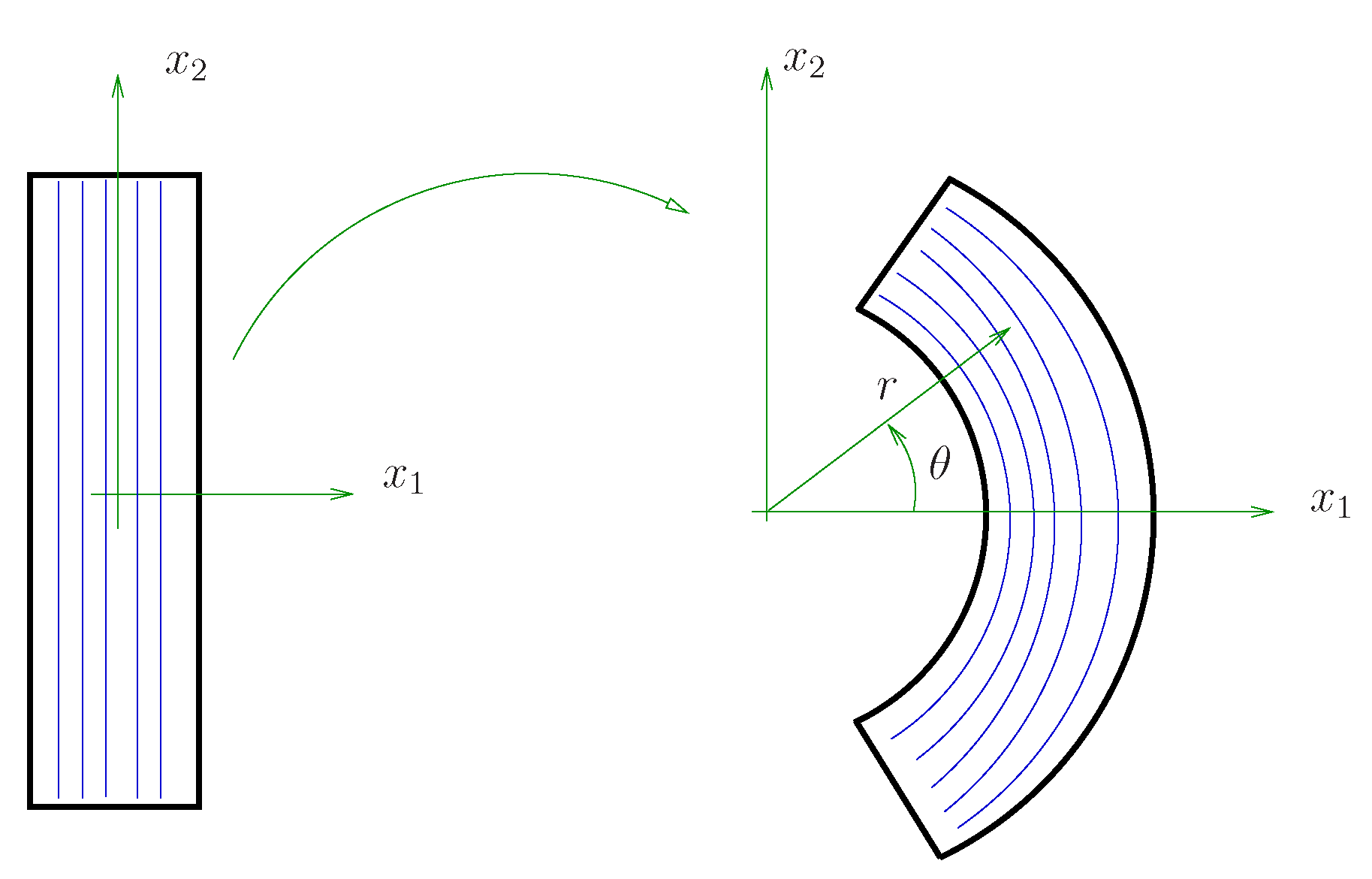
6.1. Pure Bending

A deformation of pure bending in plane strain is depicted in Figure 1, where a sector of a circular annulus defined by

$$\begin{array}{c}\hfill r=r\left(x_1\right),\theta =\theta \left(x_2\right),z=x_3,0\le x_1\le B,-L\le x_2\le L,-H\le x_3\le H\end{array}$$

(42)

is obtained via bending a rectangular slab of incompressible material: Note that $(r,\theta ,z)$ is the cylindrical polar coordinate for the current configuration and $(x_1,x_2,x_3)$ is the Cartesian referential coordinate with the basis $\{{\mathit{g}}_1,{\mathit{g}}_2,{\mathit{g}}_3={\mathit{e}}_z\}$.

The formula employed here could be used to compare our theory with experiments (for example, a three-point bending test experiment described in reference [42]).

In this case,

$$\begin{array}{c}\hfill \mathit{F}=r^{\prime }{\mathit{e}}_r\otimes {\mathit{g}}_1+r{\theta }^{\prime }{\mathit{e}}_{\theta }\otimes {\mathit{g}}_2+{\mathit{e}}_z\otimes {\mathit{g}}_3.\end{array}$$

(43)

In view of $det\mathit{F}=1$ and the conditions $\theta \left(0\right)=0$ and $r\left(A\right)=a$ at the boundary, we obtain

$$\begin{array}{c}\hfill r^2-a^2=2\chi x_1,\theta ={\displaystyle \frac{x_2}{\chi }},\chi ={\displaystyle \frac{b^2-a^2}{2B}}>0,\end{array}$$

(44)

where $r\left(B\right)=b$. Hence, in view of (3), (43) and (44), we have

$$\begin{array}{c}\hfill {\lambda }_1={\displaystyle \frac{\chi }{r}},{\lambda }_2={\displaystyle \frac{r}{\chi }},{\lambda }_3=1\end{array}$$

(45)

and the spectral basis vectors are ${\mathit{u}}_i=g_i$, ${\mathit{v}}_1={\mathit{e}}_r$, ${\mathit{v}}_2={\mathit{e}}_{\theta }$ and ${\mathit{v}}_3={\mathit{e}}_z$.

We only study the case $\mathit{a}={\mathit{g}}_2$ and $\mathit{e}={\displaystyle \frac{e_0}{r}}{\mathit{e}}_{\theta }$. Hence, ${\displaystyle {\mathit{e}}_L={\displaystyle \frac{e_0}{\chi }}}{\mathit{g}}_2$, $a_1=a_3=0$, $a_2=1$ $c_1=c_3=0$ and $c_2=1$, and clearly $\mathrm{Curl}{\mathit{e}}_L=0$ is satisfied. If we let $\overline{\mathit{F}}=\mathit{F}$, we obtain

$$\begin{array}{c}\hfill \mathit{k}=-{\mathit{g}}_1,\rho ={\displaystyle \frac{1}{r}},b_1=-1,b_2=b_3=0.\end{array}$$

(46)

The strain energy function is simplified, i.e.,

$$\begin{array}{ccc}\hfill W_{\left(T\right)}& =& \mu \sum _{i=1}^3{r}_1^2\left({\lambda }_i\right)+2{\mu }_1{r}_2^2\left({\lambda }_2\right)+{\displaystyle \frac{{\kappa }_1}{2}}{r}_3^2\left({\lambda }_2\right),\hfill \\ \hfill W_{(\Lambda )}& =& 2{\rho }^2{\mu }_2{r}_4^2\left({\lambda }_1\right)+{\rho }^4{\displaystyle \frac{{\kappa }_2}{2}}{r}_5^2\left({\lambda }_1\right)+{\rho }^2{\kappa }_3{r}_6\left({\lambda }_2\right)r_7\left({\lambda }_1\right),\hfill \\ \hfill W_{\left(E\right)}& =& c_0\left(\mathit{e}\right)r_8^2\left({\lambda }_2\right)-{\displaystyle \frac{{ϵ}_0{\mathit{e}}^2}{2{\lambda }_2^2}},W=W_{\left(T\right)}+W_{(\Lambda )}+W_{\left(E\right)}.\hfill \end{array}$$

(47)

The nonzero Cauchy stress components simply become

$$\begin{array}{c}\hfill {\sigma }_i={\lambda }_i{\displaystyle \frac{\partial W}{\partial {\lambda }_i}}-p,\end{array}$$

(48)

where ${\sigma }_1={\sigma }_{rr}$, ${\sigma }_2={\sigma }_{\theta \theta }$ and ${\sigma }_3={\sigma }_{zz}$ are cylindrical components of the Cauchy stress. The Maxwell stress simply becomes

$$\begin{array}{c}\hfill {\mathit{T}}_M={\displaystyle \frac{{\epsilon }_0{e}^2}{2r^2}}(-{\mathit{e}}_r\otimes {\mathit{e}}_r+{\mathit{e}}_{\theta }\otimes {\mathit{e}}_{\theta }-{\mathit{e}}_z\otimes {\mathit{e}}_z).\end{array}$$

(49)

Since ${\sigma }_i$ depends only on r, the equilibrium equation simply becomes

$$\begin{array}{c}\hfill {\displaystyle \frac{d{\sigma }_{rr}}{dr}}+{\displaystyle \frac{1}{r}}({\sigma }_{rr}-{\sigma }_{\theta \theta })=0.\end{array}$$

(50)

We note that in view of the Maxwell stress in (49), ${\displaystyle {\sigma }_{rr}=-{\displaystyle \frac{{\epsilon }_0{e}^2}{2b^2}}}$ at $r=b$, we then have

$$\begin{array}{c}\hfill {\sigma }_{rr}=-{\int }_r^{b}G\left(y\right)dy+{\displaystyle \frac{{\epsilon }_0{e}^2}{2b^2}},rG\left(r\right)={\lambda }_2{\displaystyle \frac{\partial W}{\partial {\lambda }_2}}-{\lambda }_1{\displaystyle \frac{\partial W}{\partial {\lambda }_1}}.\end{array}$$

(51)

Hence, we can evaluate

$$\begin{array}{c}\hfill p={\lambda }_1{\displaystyle \frac{\partial W}{\partial {\lambda }_1}}+{\int }_r^{b}G\left(y\right)dy-{\displaystyle \frac{{\epsilon }_0{e}^2}{2b^2}}.\end{array}$$

(52)

The stress–strain relations for ${\sigma }_{\theta \theta }$ and ${\sigma }_{zz}$ can now be obtained using the above p. The bending moment is

$$\begin{array}{c}\hfill \mathcal{M}={\int }_a^{b}r{\sigma }_{\theta \theta }dr\end{array}$$

(53)

and the normal force is

$$\begin{array}{c}\hfill \mathcal{N}={\int }_a^b{\sigma }_{\theta \theta }dr.\end{array}$$

(54)

Both $\mathcal{M}$ and $\mathcal{N}$ are derived per unit length in the $x_3$ direction, and applied to a section of constant $\theta$.

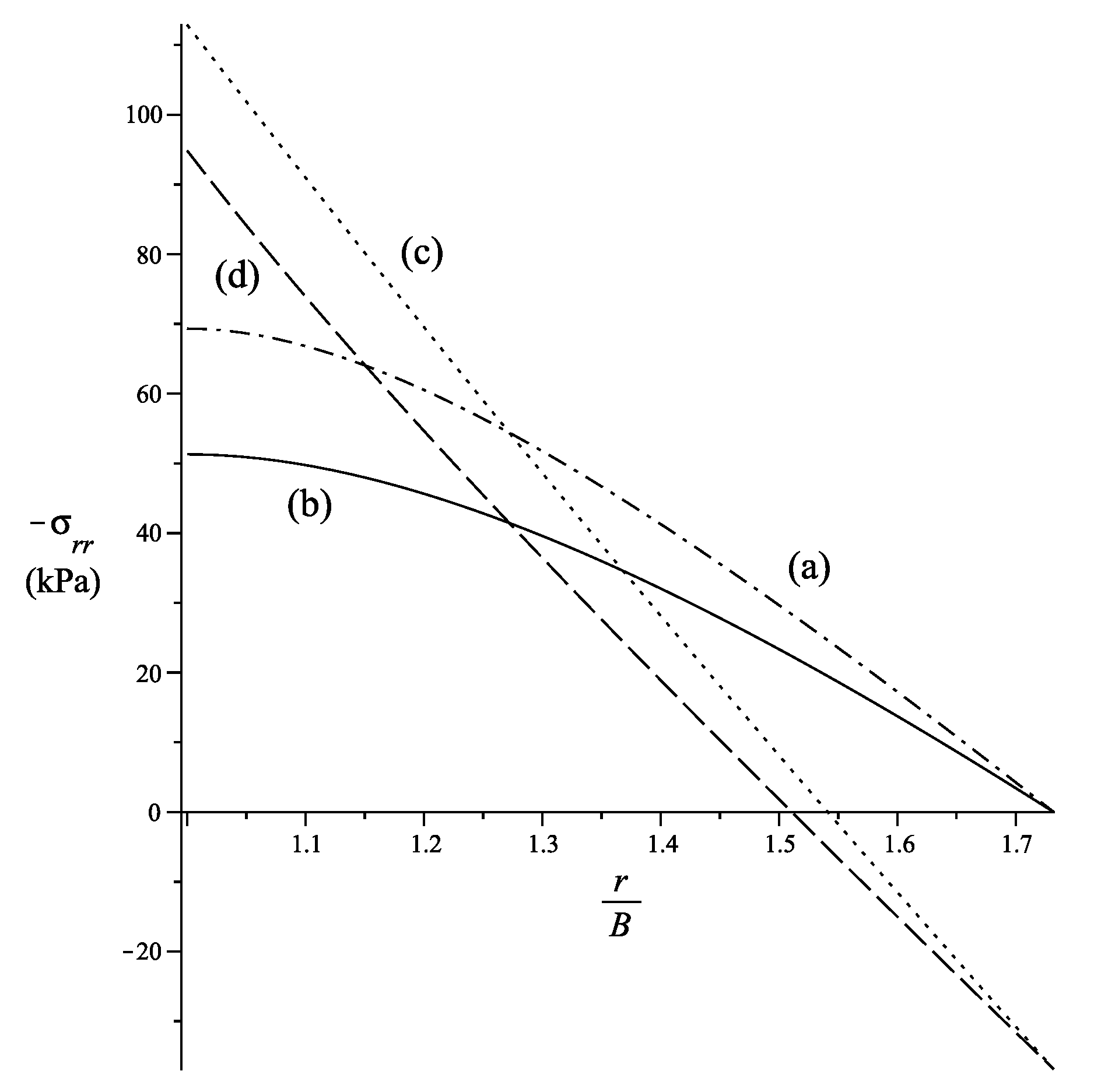
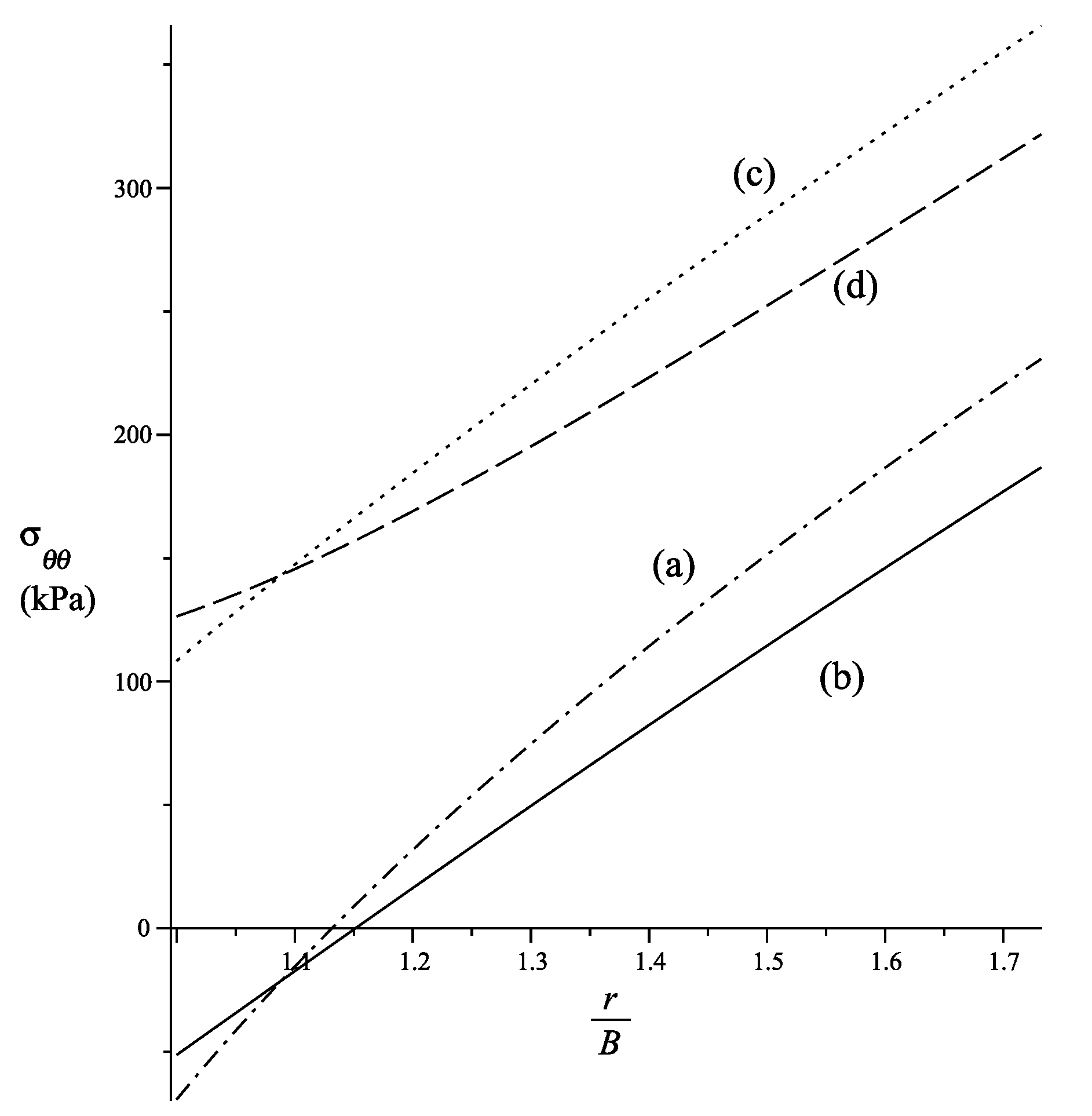
In Figure 2 and Figure 3, the behaviours of, respectively, the radial and hoop stresses are depicted using ${\displaystyle \frac{\chi }{B}}=1$, and the material is deformed to ${\displaystyle \frac{a}{B}}=1$. It is clear from these figures that the magnitude of the stresses is affected by bending fibre resistance and by the presence of an electric field.

The bending moment $\mathcal{M}$ values are

$$\begin{array}{ccc}\hfill 107.8388439& & {\mathrm{kPam}}^2,\mathrm{with} \mathrm{fibre} \mathrm{bending} \mathrm{resistance},e_0=0 \mathrm{V}/\mathrm{m};\hfill \\ \hfill 80.72073233& & {\mathrm{kPam}}^2,\mathrm{without} \mathrm{fibre} \mathrm{bending} \mathrm{resistance},e_0=0 \mathrm{V}/\mathrm{m};\hfill \\ \hfill 252.8614021& & {\mathrm{kPam}}^2,\mathrm{with} \mathrm{fibre} \mathrm{bending} \mathrm{resistance},e_0=5\times {10}^6 \mathrm{V}/\mathrm{m};\hfill \\ \hfill 225.7432905& & {\mathrm{kPam}}^2,\mathrm{without} \mathrm{fibre} \mathrm{bending} \mathrm{resistance},e_0=5\times {10}^6 \mathrm{V}/\mathrm{m}.\hfill \end{array}$$

(55)

The normal force $\mathcal{N}$ values are

$$\begin{array}{ccc}\hfill 69.32308513& & \mathrm{kPam},\mathrm{with} \mathrm{fibre} \mathrm{bending} \mathrm{resistance},e_0=0 \mathrm{V}/\mathrm{m};\hfill \\ \hfill 51.29533089& & \mathrm{kPam},\mathrm{without} \mathrm{fibre} \mathrm{bending} \mathrm{resistance},e_0=0 \mathrm{V}/\mathrm{m};\hfill \\ \hfill 176.7433952& & \mathrm{kPam},\mathrm{with} \mathrm{fibre} \mathrm{bending} \mathrm{resistance},e_0=5\times {10}^6 \mathrm{V}/\mathrm{m};\hfill \\ \hfill 158.7156409& & \mathrm{kPam},\mathrm{without} \mathrm{fibre} \mathrm{bending} \mathrm{resistance},e_0=5\times {10}^6 \mathrm{V}/\mathrm{m}.\hfill \end{array}$$

(56)

Hence, the presence of fibre bending stiffness and an electric field increases the magnitude of $\mathcal{M}$ and $\mathcal{N}$.

We note that

$$\begin{array}{c}\hfill {\mathit{d}}_L=d_1\left(x_1\right){\mathit{g}}_2,d_1\left(x_1\right)={\displaystyle \frac{{ϵ}_{0}e}{{\lambda }_2^2}}-c_0^{\prime }\left(e\right)r_8^2\left({\lambda }_2\right)\end{array}$$

(57)

which implies that $\mathrm{Div}{\mathit{d}}_L=0$, since the component of ${\mathit{d}}_L$ depends on the variable $x_1$ only.

6.2. Torsion and Extension of a Cylinder

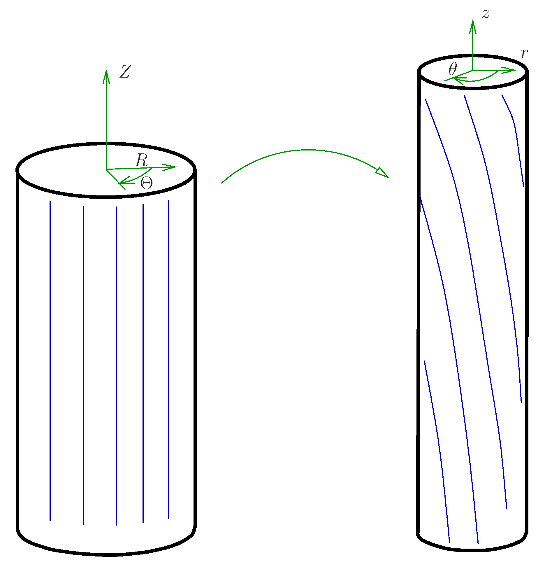
The initial geometry of an incompressible thick-walled circular cylindrical annulus is described by

$$0\le R\le A,0\le \Theta \le 2\pi ,0\le Z\le L,$$

(58)

where R, $\Theta$ and Z are reference polar coordinates with the corresponding basis $B_R=\{{\mathit{E}}_R,{\mathit{E}}_{\Theta },{\mathit{E}}_Z\}$. The boundary value problem illustrated here could be used in an experiment (see, for example, reference [43]) to verify our theoretical predictions.

The deformation is depicted in Figure 4 and is described by

$$r={\lambda }_z^{-\frac{1}{2}}R,\theta =\Theta +{\lambda }_z\tau Z,z={\lambda }_{z}Z,$$

(59)

where $\tau$ is the amount of torsional twist per unit deformed length and ${\lambda }_z$ is the axial stretch. In the above formulation, r, $\theta$ and z are cylindrical polar coordinates in the deformed configuration with the corresponding basis $B_C=\{{\mathit{e}}_r,{\mathit{e}}_{\theta },{\mathit{e}}_z\}$. Here, we have allowed ${\mathit{e}}_r={\mathit{E}}_R$, ${\mathit{e}}_{\theta }={\mathit{E}}_{\Theta }$ and ${\mathit{e}}_z={\mathit{E}}_Z$. The deformation gradient is

$$\begin{array}{c}\hfill \mathit{F}={\lambda }_z^{-1/2}{\mathit{e}}_r\otimes {\mathit{E}}_R+{\lambda }_z^{-1/2}{\mathit{e}}_{\theta }\otimes {\mathit{E}}_{\Theta }+{\lambda }_z\gamma {\mathit{e}}_{\theta }\otimes {\mathit{E}}_Z+{\lambda }_z{\mathit{e}}_z\otimes {\mathit{E}}_Z,\end{array}$$

(60)

where $\gamma =r\tau$, and in this paper, we only consider ${\lambda }_z\ge 1$. The Lagrangian principal directions are

$${\mathit{u}}_1={\mathit{E}}_R,{\mathit{u}}_2=c{\mathit{E}}_{\Theta }+s{\mathit{E}}_Z,{\mathit{u}}_3=-s{\mathit{E}}_{\Theta }+c{\mathit{E}}_Z,$$

(61)

where

$$c=cos\left(\varphi \right)=\frac{2}{\sqrt{2({\widehat{\gamma }}^2+4)+2\widehat{\gamma }\sqrt{{\widehat{\gamma }}^2+4}}},s=sin\left(\varphi \right)=\frac{\widehat{\gamma }+\sqrt{{\widehat{\gamma }}^2+4}}{\sqrt{2({\widehat{\gamma }}^2+4)+2\widehat{\gamma }\sqrt{{\widehat{\gamma }}^2+4}}},$$

(62)

with

$$\begin{array}{c}\hfill \frac{\pi }{4}\le \frac{\pi -{tan}^{-1}\left(\frac{1}{\sqrt{{\lambda }_z^3-1}}\right)}{2}\le \varphi <\frac{\pi }{2},\widehat{\gamma }=\frac{{\lambda }_z^3{\gamma }^2+{\lambda }_z^3-1}{{\lambda }_z^{\frac{3}{2}}\gamma }\ge 0,c^2-s^2=-\widehat{\gamma }cs.\end{array}$$

(63)

In the case of pure torsion, ${\lambda }_z=1$ and we have $\widehat{\gamma }=\gamma$. The principal stretches for a combined extension and torsion deformation are

$$\begin{array}{c}\hfill {\lambda }_1=\frac{1}{{\lambda }_z^{\frac{1}{2}}},{\lambda }_2=\sqrt{\frac{1}{{\lambda }_z}+\frac{s\gamma \sqrt{{\lambda }_z}}{c}},{\lambda }_3=\sqrt{\frac{1}{{\lambda }_z}-\frac{c\gamma \sqrt{{\lambda }_z}}{s}}.\end{array}$$

(64)

In this section, for simplicity, we only consider the cases when $\mathit{a}={\mathit{E}}_z$ and ${\mathit{e}}_L=e{\mathit{E}}_R$, where e is a constant. Hence, $a_1=0$, $a_2=s$, $a_3=c$, $c_2=c_3=0$ and $c_1=1$. Clearly, the relation $\mathrm{Curl}{\mathit{e}}_L=0$ is satisfied. If we let $\overline{\mathit{F}}=\mathit{F}$, and using

$$\begin{array}{c}\hfill \mathrm{Grab}\mathit{b}={\displaystyle \frac{\partial \mathit{b}}{\partial R}}\otimes {\mathit{E}}_R+{\displaystyle \frac{1}{R}}{\displaystyle \frac{\partial \mathit{b}}{\partial \Theta }}\otimes E_{\Theta }+{\displaystyle \frac{\partial \mathit{b}}{\partial Z}}\otimes {\mathit{E}}_Z,\end{array}$$

(65)

we obtain

$$\begin{array}{c}\hfill \mathit{k}=-{\mathit{E}}_R,\rho ={\displaystyle \frac{{\lambda }_z^3\gamma \tau }{\sqrt{{\lambda }_z^2(1+{\gamma }^2)}}},b_1=-1,b_2=b_3=0.\end{array}$$

(66)

The strain energy function then takes the form

$$\begin{array}{ccc}\hfill W_{\left(T\right)}& =& \mu \sum _{i=1}^3{r}_1^2\left({\lambda }_i\right)+2{\mu }_1[s^2{r}_2^2\left({\lambda }_2\right)+c^2{r}_2^2\left({\lambda }_3\right)]+{\displaystyle \frac{{\kappa }_1}{2}}{[s^2{r}_3\left({\lambda }_2\right)+c^2{r}_3\left({\lambda }_3\right)]}^2,\hfill \\ \hfill W_{(\Lambda )}& =& 2{\rho }^2{\mu }_2{r}_4^2\left({\lambda }_1\right)+{\rho }^4{\displaystyle \frac{{\kappa }_2}{2}}{r}_5^2\left({\lambda }_1\right)+{\rho }^2{\kappa }_3[s^2{r}_6\left({\lambda }_2\right)+c^2{r}_6\left({\lambda }_3\right)]r_7\left({\lambda }_1\right),\hfill \\ \hfill W_{\left(E\right)}& =& c_0\left(\mathit{e}\right)r_8^2\left({\lambda }_1\right)-{\displaystyle \frac{{\epsilon }_0{e}^2}{2{\lambda }_1^2}}.\hfill \end{array}$$

(67)

The Maxwell stress is

$$\begin{array}{c}\hfill {\mathit{T}}_M={\displaystyle \frac{{\epsilon }_0{\lambda }_z{e}^2}{2}}({\mathit{e}}_r\otimes {\mathit{e}}_r-{\mathit{e}}_{\theta }\otimes {\mathit{e}}_{\theta }+{\mathit{e}}_z\otimes {\mathit{e}}_z).\end{array}$$

(68)

The total Cauchy stress is

$$\begin{array}{c}\hfill \mathit{T}=2\mathit{F}{\displaystyle \frac{\partial W}{\partial \mathit{C}}}{\mathit{F}}^T-pI.\end{array}$$

(69)

In view of $\mathit{a}\equiv {[0,0,1]}^{\mathit{T}}$, we have $a_1=0$, $a_2=s$ and $a_3=c$ and

$$\begin{array}{c}\hfill \mathit{T}={\sigma }_{rr}{\mathit{e}}_r\otimes {\mathit{e}}_r+{\sigma }_{\theta \theta }{\mathit{e}}_{\theta }\otimes {\mathit{e}}_{\theta }+{\sigma }_{zz}{\mathit{e}}_z\otimes {\mathit{e}}_z+{\sigma }_{z\theta }({\mathit{e}}_z\otimes {\mathit{e}}_{\theta }+{\mathit{e}}_{\theta }\otimes {\mathit{e}}_z),\end{array}$$

(70)

where

$$\begin{array}{ccc}& & {\sigma }_{\theta \theta }=2\left[{\displaystyle \frac{l_2{c}^2+l_3{s}^2-2l_{4}cs}{{\lambda }_z}}+2\sqrt{{\lambda }_z}\gamma ((l_2-l_3)cs+l_4(c^2-s^2))+{\lambda }_z^2{\gamma }^2(l_2{s}^2+l_3{c}^2+2l_{4}cs)\right]-p,\hfill \\ & & {\sigma }_{z\theta }=2\left[\sqrt{{\lambda }_z}((l_2-l_3)cs+l_4(c^2-s^2))+{\lambda }_z^2\gamma (l_2{s}^2+l_3{c}^2+2l_{4}cs)\right],\hfill \\ & & {\sigma }_{zz}=2{\lambda }_z^2\left(l_2{s}^2+l_3{c}^2+2l_{4}cs\right)-p,{\sigma }_{rr}={\displaystyle \frac{2l_1}{{\lambda }_z}}-p,\hfill \end{array}$$

(71)

where

$$\begin{array}{c}\hfill l_i={\left({\displaystyle \frac{\partial W}{\partial \mathit{C}}}\right)}_{ii},i=1,2,3,l_4={\left({\displaystyle \frac{\partial W}{\partial \mathit{C}}}\right)}_{23}.\end{array}$$

(72)

The normal force per unit deformed area N and the torque per unit deformed area $\mathcal{M}$ applied at the ends of the cylinder are as follows:

$$N={\displaystyle \frac{2}{a^2}}{\int }_0^a{\sigma }_{zz}r\mathrm{d}r,\mathcal{M}={\displaystyle \frac{2}{a^2}}{\int }_0^a{\sigma }_{z\theta }{r}^2\mathrm{d}r,a={\displaystyle \frac{A}{\sqrt{{\lambda }_z}}}.$$

(73)

To remove p in (73), we use the equilibrium relation

$$\begin{array}{c}\hfill {\sigma }_{rr}+{\sigma }_{\theta \theta }=\frac{1}{r}\frac{\mathrm{d}\left(r^2{\sigma }_{rr}\right)}{\mathrm{d}r}.\end{array}$$

(74)

and re-express (73) as

$$N={\displaystyle \frac{1}{a^2}}{\int }_0^a(2{\sigma }_{zz}-{\sigma }_{rr}-{\sigma }_{\theta \theta })r\mathrm{d}r+{\displaystyle \frac{{\epsilon }_0{\lambda }_z{e}^2}{2}}.$$

(75)

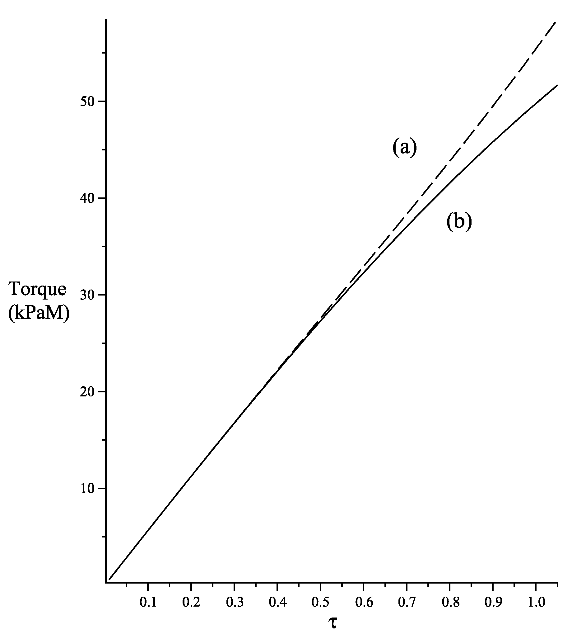
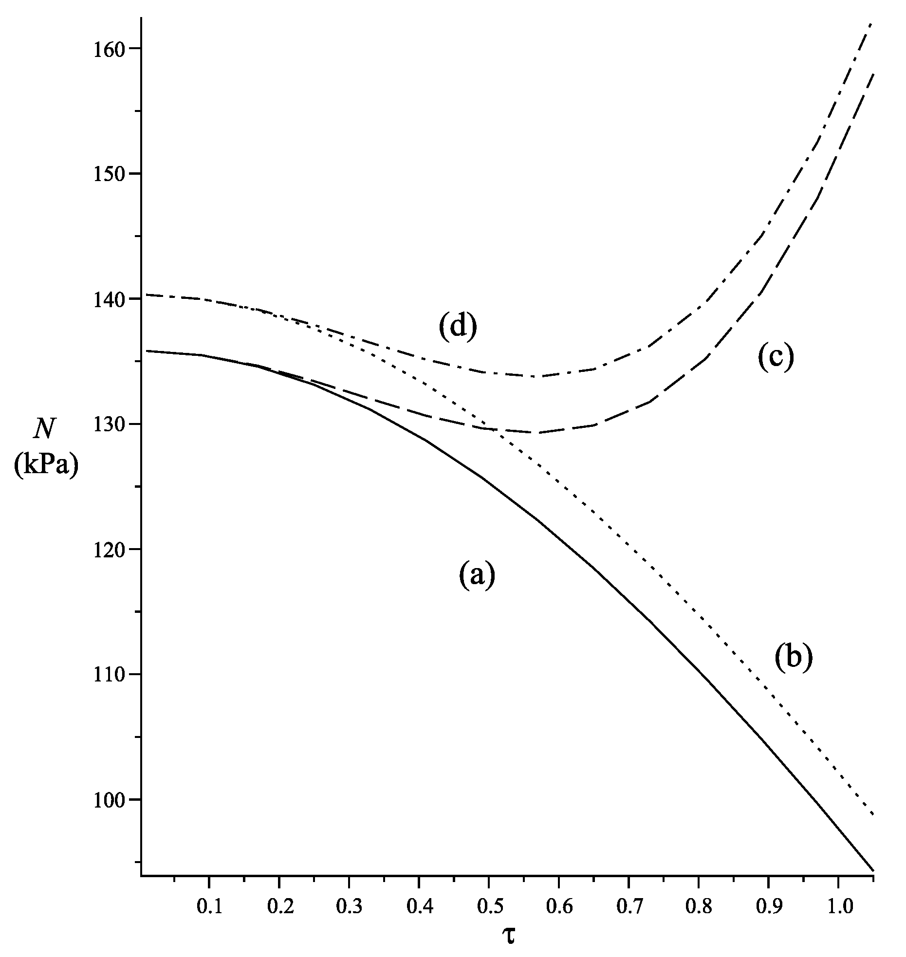
It is clear from Figure 5 that for an axial stretch ${\lambda }_z=1.5$, we require more torque to twist an elastic solid cylinder with fibre bending stiffness, and the torque is independent of the electric field ${\mathit{e}}_L=e{\mathit{E}}_R$. However, in the case of the normal force (see Figure 6), the presence of an electric field and fibre bending stiffness increases the magnitude of the normal force and changes its behaviour.

Since $W_{\left(E\right)}$ depends only on the constant principal stretch ${\lambda }_1$ (see Equation (67)), it is clear that the property $\mathrm{Div}{\mathit{d}}_L=0$ is satisfied.

7. Conclusions

We have modelled bending resistance of EAPs due to changes in the curvature of the fibres without using the second gradient theory. In view of this, our proposed constitutive equation is simpler (as shown in Section 4 and Section 5) than the second-gradient constitutive equations given in the literature; solving boundary value problems using our model is also simpler, as exemplified in Section 6. Our model does not contain contact torques (which is required in a second-gradient model), and hence, the proposed model is more realistic in the sense that contact torques do not exist in deformations of nonpolar carbon fibre-reinforced EAPs. Our constitutive equation uses recently developed spectral invariants (see Section 4.1) that are attractive and useful for experimental designs. The boundary value problem results in Section 6 indicate that our model manages to simulate fibre bending stiffness. In the near future, stable numerical decoupling strategies will be developed, whereas a level set description can be used to model the fibre direction [44,45,46]. FEM solutions of the proposed model will be obtained, and we will extend this model to EAPs that are reinforced with a family of two fibres.

References

- Wu, Z.; Lin, B.; Fan, J.; Zhao, J.; Zhang, Q.; Li, L. Effect of Dielectric Relaxation of Epoxy Resin on Dielectric Loss of Medium-Frequency Transformer. IEEE Trans. Dielectr. Electr. Insul. 2022, 29, 1651–1658. [Google Scholar] [CrossRef]
- Huang, Z.; Luo, P.; Zheng, H.; Lyu, Z.; Ma, X. Novel one-dimensional V3S4@NC nanofibers for sodium-ion batteries. J. Phys. Chem. Solids 2023, 172, 111081. [Google Scholar] [CrossRef]
- Cao, K.; Wang, B.; Ding, H.; Lv, L.; Dong, R.; Cheng, T.; Gong, F. Improving Physical Layer Security of Uplink NOMA via Energy Harvesting Jammers. IEEE Trans. Inf. Forensics Secur. 2021, 16, 786–799. [Google Scholar] [CrossRef]
- Song, Z.; Shao, X.; Wu, W.; Liu, Z.; Yang, M.; Liu, M.; Wang, H. Structures and Stabilities of Carbon Chain Clusters Influenced by Atomic Antimony. Molecules 2023, 28, 1358. [Google Scholar] [CrossRef] [PubMed]
- Shi, M.; Wang, R.; Li, L.; Chen, N.; Xiao, P.; Yan, C.; Yan, X. Redox-Active Polymer Integrated with MXene for Ultra-Stable and Fast Aqueous Proton Storage. Adv. Funct. Mater. 2022, 33, 2209777. [Google Scholar] [CrossRef]
- Xiao, X.; Zhang, Q.; Zheng, J.; Li, Z.; Yan, X. Analytical model for the nonlinear buckling responses of the confined polyhedral FGP-GPLs lining subjected to crown point loading. Eng. Struct. 2023, 282, 115780. [Google Scholar] [CrossRef]
- Bar-Cohen, Y. Electro-active polymers: Current capabilities and challenges. In Proceedings of the 4th Electroactive Polymer Actuators and Devices (EAPAD) Conference, 9th Smart Structures and Materials Symposium, San Diego, CA, USA, 11 July 2002. [Google Scholar]
- Chukov, D.; Nematulloev, S.; Zadorozhnyy, M.; Tcherdyntsev, V.; Stepashkin, A.; Zherebtsov, D. Structure, mechanical and thermal properties of polyphenylene sulfide and polysulfone impregnated carbon fiber composites. Polymers 2019, 11, 684. [Google Scholar] [CrossRef]
- Linul, E.; Lell, D.; Movahedi, N.; Codrean, C.; Fiedler, T. Compressive properties of Zinc Syntactic Foams at elevated temperatures. Compos. Part B Eng. 2019, 167, 122–134. [Google Scholar] [CrossRef]
- Sherif, G.; Chukov, D.; Tcherdyntsev, V.; Torokhov, V. Effect of formation route on the mechanical properties of the polyethersulfone composites reinforced with glass fibers. Polymers 2019, 11, 1364. [Google Scholar] [CrossRef]
- Yashas Gowda, T.G.; Sanjay, M.R.; Subrahmanya Bhat, K.; Madhu, P.; Senthamaraikannan, P.; Yogesha, B. Polymer matrix-natural fiber composites: An overview. Cogent. Eng. 2018, 5, 1446667. [Google Scholar] [CrossRef]
- Clyne, T.W.; Hull, D. An Introduction to Composite Materials, 3rd ed.; Cambridge University Press: Cambridge, UK, 2019. [Google Scholar]
- Monteiro, S.N.; de Assis, F.S.; Ferreira, C.L.; Simonassi, N.T.; Weber, R.P.; Oliveira, M.S.; Colorado, H.A.; Pereira, A.C. Fique fabric: A promising reinforcement for polymer composites. Polymers 2018, 10, 246. [Google Scholar] [CrossRef] [PubMed]
- Movahedi, N.; Linul, E. Quasi-static compressive behavior of the ex-situ aluminum-alloy foam-filled tubes under elevated temperature conditions. Mater. Lett. 2017, 206, 182–184. [Google Scholar] [CrossRef]
- Zagho, M.M.; Hussein, E.A.; Elzatahry, A.A. Recent overviews in functional polymer composites for biomedical applications. Polymers 2018, 10, 739. [Google Scholar] [CrossRef] [PubMed]
- Gizzi, A.; Ruiz-Baier, R.; Rossi, S.; Laadhari, A.; Cherubini, C.; Filippi, S. A three-dimensional continuum model of active contraction in single cardiomyocytes. In Modeling the Heart and the Circulatory System; Springer International Publishing: Cham, Switzerland, 2015; pp. 157–176. [Google Scholar] [CrossRef]
- Shariff, M.H.B.M. Physical invariant strain energy function for passive myocardium. J. Biomech. Model. Mechanobiol. 2012, 12, 215–223. [Google Scholar] [CrossRef]
- Shariff, M.H.B.M. On the spectral constitutive modelling of transversely isotropic soft tissue: Physical invariants. Int. J. Eng. Sci. 2017, 120, 199–219. [Google Scholar] [CrossRef]
- Shariff, M.H.B.M.; Bustamante, R.; Merodio, J. A nonlinear electro- elastic model with residual stresses and a preferred direction. Math. Mech. Solids 2020, 25, 838–865. [Google Scholar] [CrossRef]
- Shariff, M.H.B.M.; Bustamante, R.; Merodio, J. A nonlinear con- stitutive model for a two preferred direction electro-elastic body with residual. Int. J.-Non-Linear Mech. 2020, 119, 103352. [Google Scholar] [CrossRef]
- Ferreti, M.; Madeo, A.; Dell’isola, F.; Boisse, P. Modeling the onset of shear boundary layers in fibrous composite reinforcements by second gradient theory. Z. Angew. Math. Phys. 2013, 65, 587–612. [Google Scholar] [CrossRef]
- Pipkin, A.C. Stress analysis for fiber-reinforced materials. Adv. Appl. Mech. 1979, 19, 1–51. [Google Scholar]
- Shariff, M.H.B.M.; Merodio, J. Residually stressed fiber reinforced solids: A spectral approach. Materials 2020, 13, 4076. [Google Scholar] [CrossRef]
- Spencer, A.J.M. Deformations of Fibre-Reinforced Materials; Oxford University Press: Oxford, UK, 1972. [Google Scholar]
- Shariff, M.H.B.M.; Merodio, J.; Bustamante, R. Finite deformations of fibre bending stiffness: A spectral approach. J. Appl. Comput. Mech. 2022, 8, 1332–1342. [Google Scholar]
- Shariff, M.H.B.M.; Merodio, J.; Bustamante, R. Nonlinear elastic constitutive relations of residually stressed composites with stiff curved fibres. Appl. Math. Mech. 2022, 43, 1515–1530. [Google Scholar] [CrossRef]
- Soldatos, K.P.; Shariff, M.H.B.M.; Merodio, J. On the Constitution of Polar Fibre-reinforced Materials. Mech. Adv. Mater. Struct. 2020, 28, 2255–2266. [Google Scholar] [CrossRef]
- Spencer, A.J.M.; Soldatos, K.P. Finite deformations of fibre-reinforced elastic solids with fibre bending stiffness. Int. J.-Non-Linear Mech. 2007, 42, 355–368. [Google Scholar] [CrossRef]
- Steigmann, D. Theory of elastic solids reinforced with fibers resistant to extension, flexure and twist. Int. J. Non-Linear Mech. 2012, 47, 734–742. [Google Scholar] [CrossRef]
- Hadjesfandiari, A.R.; Dargush, G.F. Couple stress theory for solids. Int. J. Solids Struct. 2011, 48, 2496–2510. [Google Scholar] [CrossRef]
- Hadjesfandiari, A.R.; Dargush, G.F. Evolution of generalized couple-stress continuum theories:a critical analysis. arXiv 2015, arXiv:1501.03112. [Google Scholar]
- Neff, P.; Münch, I.; Ghiba, I.; Madeo, A. On some fundamental misunderstandings in the indeterminate couple stress model. A comment on recent papers of A.R. Hadjesfandiari and G.F. Dargush. Int. J. Solids Struct. 2016, 81, 233–243. [Google Scholar] [CrossRef]
- Shariff, M.H.B.M. A generalized strain approach to anisotropic elasticity. Sci. Rep. 2022, 12, 172. [Google Scholar] [CrossRef]
- Shariff, M.H.B.M.; Bustamante, R.; Hossain, M. A Generalised Time-Dependent Mathematical Formulation for Magnetoelectrically Coupled Soft Solids at Finite Strains. Symmetry 2023, 15, 628. [Google Scholar] [CrossRef]
- Dorfmann, A.; Ogden, R.W. Nonlinear electroelasticity. Acta Mech. 2005, 174, 167–183. [Google Scholar] [CrossRef]
- Kovetz, A. Electromagnetic Theory; Oxford University Press: Oxford, UK, 2000. [Google Scholar]
- Ogden, R.W.; Steigmann, D.J. Mechanics and Electrodynamics of Magneto- and Electro-Elastic Materials; Springer: Wien, Austria, 2011; Volume 527, CISM Courses and Lectures Series. [Google Scholar]
- Shariff, M.H.B.M.; Merodio, J.; Bustamante, R. A non-second-gradient model for nonlinear elastic bodies with fibre stiffness. Sci. Rep. 2023, 13, 6562. [Google Scholar] [CrossRef] [PubMed]
- Shariff, M.H.B.M. Anisotropic separable free energy functions for elastic and non-elastic solids. Acta Mech. 2016, 227, 3213–3237. [Google Scholar] [CrossRef]
- Shariff, M.H.B.M. On the Smallest Number of Functions Representing Isotropic Functions of Scalars, Vectors and Tensors. Q. J. Mech. Appl. Math. 2023. [Google Scholar] [CrossRef]
- Morrow, D.A.; Donahue, T.L.H.; Odegard, G.M.; Kaufman, K.R. Transversely isotropic tensile material properties of skeletal muscle tissue. J. Mech. Behav. Biomed. Mater. 2010, 3, 124–129. [Google Scholar] [CrossRef]
- Mathieu, S.; Hamila, N.; Bouillon, F.; Boisse, P. Enhanced modeling of 3D composite preform deformations taking into account local fiber bending stiffness. Compos. Sci. Technol. 2015, 117, 322–333. [Google Scholar] [CrossRef]
- Lu, W.-Y.; Jin, H.; Foul, J.W.; Ostien, J.; Kramer, S.L.; Jones, A. Solid cylinder torsion for large shear deformation and failure of engineering materials. Exp. Mech. 2021, 61, 307–320. [Google Scholar] [CrossRef]
- Laadhari, A.; Saramito, P.; Misbah, C.; Székely, G. Fully implicit methodology for the dynamics of biomembranes and capillary interfaces by combining the level set and Newton methods. J. Comput. Phys. 2017, 343, 271–299. [Google Scholar] [CrossRef]
- Laadhari, A.; Székely, G. Fully implicit finite element method for the modeling of free surface flows with surface tension effect. Int. J. Numer. Methods Eng. 2017, 111, 1047–1074. [Google Scholar] [CrossRef]
- Laadhari, A. Implicit finite element methodology for the numerical modeling of incompressible two-fluid flows with moving hyperelastic interface. Appl. Math. Comput. 2018, 333, 376–400. [Google Scholar] [CrossRef]
- Ogden, R.W. Non-Linear Elastic Deformations; Ellis Horwood: Chichester, UK, 1984. [Google Scholar]
Figure 1.
Bending of a rectangular block into a sector of a cylindrical tube.
Figure 2.
Radial behaviour of stress . (a) Elastic solid with fibre bending resistance. V/m. (b) Elastic solid with no fibre bending resistance. V/m. (c) Elastic solid with fibre bending resistance. V/m. (d) Elastic solid with no fibre bending resistance. V/m.
Figure 3.