Ranking Method of Intuitionistic Fuzzy Numbers and Multiple Attribute Decision Making Based on the Probabilistic Dominance Relationship

Abstract

The uncertainty of intuitionistic fuzzy numbers (IFNs) is further enhanced by the existence of the degree of hesitation (DH). The shortcomings of existing researches are mainly reflected in the following situations: when comparing IFNs, the comparison rules of IFNs are difficult to apply to the comparison of any two IFNs, or the relevant methods do not fully consider the uncertainty expressed by DH. Thus, the rationality of the decision results needs to be improved. On the other hand, multi-attribute decision making (DADM) based on IFNs is often not objective due to the need to determine the attribute weight. Moreover, the strict condition of attribute aggregation of classical dominance relation makes it a method that fails considering the practical application. Aiming at the comparison problem of IFNs, this paper takes probability conversion as the starting point and proposes an IFN comparison method based on the area method, which can better deal with the comparison problem of “either superior or inferior” IFNs. In addition, aiming at the MADM problem of an intuitionistic fuzzy information system, we propose an intuitionistic fuzzy probabilistic dominance relation model and construct the MADM method under the probabilistic dominance relation. The series properties of IFNs and probabilistic dominance relation were summarized and proved, which theoretically ensured the scientificity and rigor of the method. The results show that the comparison and ranking method of IFNs proposed in this paper can be applied to the comparison of any two IFNs, and the dominance degree of IFNs is presented in the form of probability, which is more flexible and practical than the classical method. The probabilistic dominance relation method based on IFNs avoids the problem of determining attribute weights subjectively or objectively, and the decision maker can reflect decision preference by adjusting decision parameters to better match the actual problem. The application of this model to a campus express site evaluation further verifies the feasibility of the proposed method and the rationality of the results. In addition, various extension problems of the model and method proposed in this paper are discussed, which pave the way for future related research. This paper constructs a complete decision-making framework through theoretical analysis and application from practical problems, which provides a reference for enriching and improving uncertain decision-making theory and the MADM method.

1. Introduction

Since its birth in 1965, fuzzy sets theory [1] has been widely concerned by the academic community and has been widely applied in various fields subsequently as a uncertainty quantification model and method [2,3]. At present, the research on fuzzy sets theory in the academic circle has tended to be mature, and many new concepts and models of fuzzy sets extension have appeared, such as intuitionistic fuzzy sets (IFS) [4,5], hesitant fuzzy sets [6,7], etc. Some scholars integrate fuzzy sets theory with other theories to solve new problems, such as fuzzy rough sets [8,9,10,11], rough fuzzy sets [12,13,14], fuzzy soft sets [15], Pythagorean fuzzy sets [16,17], etc. Regarding the application of fuzzy sets, relevant scholars have also conducted extensive discussions, such as applying intuitionistic fuzzy sets to ensemble learning [18] and emergency logistics plan decision [19], applying hesitant fuzzy sets to sequence recognition [20] and product quality management [21], applying interval fuzzy sets to risk management [22] and transportation problems [23], etc., and achieving fruitful results in a series of studies.

IFS increase the uncertainty of information expression and applicability to practical problems because the uncertainty of fuzzy sets is described by the degree of membership (DM) and degree of non-membership (DN). Therefore, many scholars have conducted researches on IFS, such as distance measure [24,25,26] and similarity measure [27]. In addition, the model generalization of IFS is also studied, such as interval type IFS [28], Atanassov-type intuitionistic fuzzy [29], intuitionistic fuzzy soft sets [30,31], intuitionistic fuzzy rough sets [32,33], intuitionistic fuzzy set and three-way decision [34,35,36,37], intuitionistic fuzzy set and dominance relationship [38,39], and other series of achievements. At present, IFS have achieved good application results in fault diagnosis [40], multi-attribute decision-making [41], incomplete data decision-making [42], deep learning [43], imbalance learning [44], and other fields.

However, it is precisely because of the introduction of the degree of non-membership (DN) and the degree of hesitation (DH) in IFS, and there is no unified standard for the treatment of DH in the academic circle, so the comparison of intuitionistic fuzzy numbers (IFNs) has become a problem that researchers continue to explore. Atanassov K [4] defined the inclusion relation of fuzzy sets from the perspective of sets. Wei C P et al. [45] believed that the uncertainty of IFS was reflected in fuzziness and intuitionality. The fuzziness was determined by the difference between its DM and DN, while the intuitionality was determined by its DH, and the entropy measurement formula of IFS was proposed based on this. Sevastjanov P [46] proposed a new comparison method for intuitionistic fuzzy numbers that can deal with real, interval and fuzzy values. Some scholars often do not consider the influence of DH when measuring IFS. For example, Wang Y [47] and Zhao F X [48] only measured the distance between IFS with the difference between DM and DN; Li YH et al. [49] proposed a unified ranking method of intuitionistic fuzzy numbers and Pythagorean fuzzy numbers based on area characterization, but they also did not consider the influence of DH. Ye J [50] defined cosine similarity of IFS, but did not consider the influence of DH, so it is easy to get unreasonable comparison results. Xie J M et al. [51] put the DH in the same position as the DM and DN when considering the distance measure. Xu C L et al. [52] equally divided the DH into the DM and the DN, and proposed its distance measure by constructing a four-dimensional space.

In summary, the current research on IFS mainly has the following deficiencies: First, most literature does not consider the DH enough, or choose to ignore the DH, which may lead to information loss and unreasonable decision making. In other studies, DM, DN, and DH are processed in the same way. However, as DH is not completely independent of DM and DN, information redundancy will be caused to a certain extent. Second, most research results based on the integration of IFS and rough sets consider the inclusion relationship between fuzzy sets from the perspective of sets, calculate the upper approximation and lower approximation of concepts, or take classification as the purpose; in contrast, there are few studies for the purpose of evaluation and ranking.

Given the current academic research on IFS, this paper proposes a comparison method of intuitionistic fuzzy numbers considering the DH and then constructs a MADM method for intuitionistic fuzzy numbers based on probabilistic dominance relations. The main contributions of this paper are as follows:

(1) In view of the problem that the comparison and measurement of IFNs in the current research do not fully consider the DH, this paper proposes a comparison and ranking method of IFNs based on DN conversion, and by constructing the number of fuzzy intervals, the comparison of intervals based on the geometric area method is carried out and finally converted into the comparison probability of IFNs. This method can be applied to the comparison of any two IFNs, and fully considers the influence of the size of DH on the comparison of IFNs, expands the comparison method of IFNs, and obtains more reasonable results.

(2) The classical rough sets model of dominance relation often faces failure in practical decision-making problems due to the requirement of the construction of its dominance class to satisfy the condition that all attributes are simultaneously dominant. Therefore, for intuitionistic fuzzy information systems, this paper proposes a MADM method based on probabilistic dominance relations. By setting parameters α and β as the threshold of IFNs comparison and multi-attribute dominance class construction, respectively, the method can effectively solve the situation that the classical dominance relation is easy to fail, which makes the method more widely applied and robust. In addition, the method of element comparison based on the dominance class is improved and the decision steps are given. It is helpful to further develop the theory and method of uncertain decision-making theory and method based on fuzzy sets and rough sets, and improve the theory and application research of MADM.

The following chapters of this paper are arranged as follows: Section 2 is a review of basic knowledge, Section 3 is a comparison and ranking method for IFNs based on probability conversion and the area method, Section 4 is an intuitionistic fuzzy probabilistic dominance relationship and the MADM method, Section 5 is a case application analysis, Section 6 is a discussion, and Section 7 is a conclusion.

2. Basic Knowledge

In this section, the basic concept of IFS is reviewed briefly to lay a foundation for subsequent research.

Definition 1.

([4]). Let $U$ be a non-empty finite universe, and an IFS $A$ on $U$ is defined as $A=\{x,{\mu }_A(x),{\nu }_A(x)|x\in U\}$, where ${\mu }_A(x),{\nu }_A(x)$ indicate the degree of membership (DM) and degree of non-membership (DN) that element $x$ in $U$ belongs to IFS $A$, and for $\forall x\in U$, $0\le {\mu }_A(x)+{\nu }_A(x)\le 1$, ${\mu }_A$:$U\to [0,1]$ and ${\nu }_A$: $U\to [0,1]$ represent membership functions and non-membership functions of $U$ on $A$, respectively. Let ${\pi }_A(x)=1-{\mu }_A(x)-{\nu }_A(x)$ be the degree of hesitation (DH) of $U$ for set $A$, and $0\le {\pi }_A(x)\le 1$ is obvious. For $\forall x\in U$, $A(x)=({\mu }_A(x),{\nu }_A(x))$ is the intuitionistic fuzzy number (IFN) of $U$ under set $A$.

For the sake of simplification, $x=(\mu ,\nu )$ is generally used to represent the IFN; then, $0\le \mu \le 1$, $0\le \nu \le 1$ and $0\le \mu +\nu \le 1$.

Definition 2.

([38]). Let $x_1=({\mu }_1,{\nu }_1)$ and $x_2=({\mu }_2,{\nu }_2)$ be two IFNs, then $x_1\le x_2$ if and only if ${\mu }_1\le {\mu }_2$ and ${\nu }_1\ge {\nu }_2$. In particular, $x_1=x_2$ if and only if ${\mu }_1={\mu }_2$ and ${\nu }_1={\nu }_2$.

Example 1.

If  $x_1=(0.2,0.5)$,  $x_2=(0.3,0.3)$  and  $x_3=(0.4,0.4)$  are three IFNs, then it can be seen from Definition 2 that  $x_1\le x_2$  and  $x_1\le x_3$  are valid, but  $x_2$  and  $x_3$  cannot be compared according to Definition 2.

As shown in Example 1, there are two problems in the comparison of IFNs. First, this rule cannot give comparison results for any two IFNs, which greatly limits the application of IFNs in MADM. Secondly, for the IFNs that can be compared according to Definition 2, the comparison results are often irrational. This is because the existence of DH makes IFNs have greater uncertainty. If the DH is converted into DM or DN under certain conditions, the conclusion of $x_1\le x_2$ is not always valid. If the DH of $x_1$ is converted into DM and the DH of $x_2$ is converted into DN, namely $\mu ({x_1}^{\prime })=\mu (x_1)+\pi (x_1)=0.2+0.3=0.5$, $\nu ({x_2}^{\prime })=\nu (x_2)+\pi (x_2)=0.3+0.4=0.7$, then ${x_1}^{\prime }=(0.5,0.5)$ and ${x_2}^{\prime }=(0.3,0.7)$ are available. Obviously, the comparison result at this time should be ${x_1}^{\prime }>{x_2}^{\prime }$, although this conversion is not an inevitable result. However, the above example at least shows that there is a possibility of $x_1>x_2$, and it cannot be directly determined that $x_1\le x_2$ is satisfied with ${\mu }_1\le {\mu }_2$ and ${\nu }_1\ge {\nu }_2$.

3. Comparison of IFNs Based on the Area Method

Definition 3.

Let  $x_1=({\mu }_1,{\nu }_1)$ and $x_2=({\mu }_2,{\nu }_2)$ be two IFNs satisfying ${\mu }_1+{\nu }_1=1$, ${\mu }_2+{\nu }_2=1$, namely ${\pi }_1=1-{\mu }_1-{\nu }_1=0$, ${\pi }_2=1-{\mu }_2-{\nu }_2=0$. Therefore, $x_1\le x_2$ if and only if ${\mu }_1\le {\mu }_2$ and ${\nu }_1\ge {\nu }_2$. In particular, $x_1=x_2$ if and only if ${\mu }_1={\mu }_2$ and ${\nu }_1={\nu }_2$.

On the basis of Definition 2, Definition 3 makes a further strictly defined, that is, when there is no DH in IFNs, the comparison of IFNs can be made according to Definition 2.

In fact, in Definition 3, if ${\mu }_1+{\nu }_1=1$ and ${\mu }_2+{\nu }_2=1$ are satisfied, then there will be ${\nu }_1\ge {\nu }_2$ when ${\mu }_1\le {\mu }_2$. Therefore, for IFNs without DH, the IFN can be sorted by the comparison of DM directly.

Definition 4.

Let  $x=(\mu ,\nu )$  be an IFN, $\pi =1-\mu -\nu$. For $\forall \alpha \in [0,1]$, let $N_{\alpha }(x)=(\mu +\alpha \pi ,\nu +(1-\alpha )\pi )$ be an $\alpha$-probability conversion of the IFN of $x$. Obviously, $N_{\alpha }(x)=({\mu }_{\alpha },{\nu }_{\alpha })$ satisfies ${\mu }_{\alpha }+{\nu }_{\alpha }=1$.

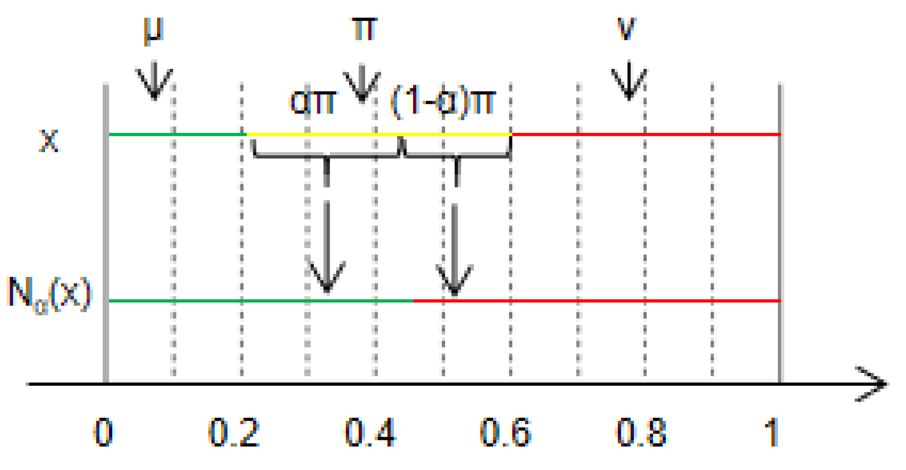
According to Definition 4, the DH of IFNs can be further clarified and converted into DM or DN of fuzzy numbers. As shown in Figure 1, the part near the left expresses the concept of certainty belonging, namely DM; the part near the right expresses the concept of certainty unbelonging, namely DN; and the middle part expresses the concept of uncertainty, namely DH. According to the assumption of probability conversion, if we convert part of π of DH into DM, the part of DM will become larger, and if we convert another part of π of DH into DN, the part of DN will also become larger. Through this probability conversion, the uncertain attribution problem of IFNs is eliminated to a certain extent, so as to enhance the comparability of IFNs.

It can be seen from Definition 4 that when $\alpha =0$, $N_0(x)=(\mu ,\nu +\pi )$, that is all the DH is converted into DN, then the degree of “non-belonging” reaches the maximum. When $\alpha =1$, $N_1(x)=(\mu +\pi ,\nu )$, that is the DH is completely converted into the DM, then the degree of “belonging” reaches the maximum. When $\alpha \in (0,1)$, the DH $\pi$ is divided into two parts, which are converted into DM and DN using $\alpha \pi$ and $(1-\alpha )\pi$, respectively.

Although all IFNs can be converted into another IFNs without DH according to Definition 4, then all IFNs without DH can be compared and sorted according to Definition 3. However, the actual problem is not so simple, because the conversion probability $\alpha$ is difficult to determine; in other words, when the value of $\alpha$ is different, different comparison and sorting results will be obtained, as shown in Example 2.

Example 2.

Let $x_1=(0.3,0.4)$ and $x_2=(0.4,0.5)$ be two IFNs. Obviously, $x_1$ and $x_2$ cannot be compared according to Definition 2. Take $\alpha =0,0.5,1$ respectively, then:

$N_0(x_1)=(0.3,0.7)$, $N_0(x_2)=(0.4,0.6)$, there is $N_0(x_1)<N_0(x_2)$.

$N_{0.5}(x_1)=(0.45,0.55)$, $N_{0.5}(x_2)=(0.45,0.55)$, there is $N_{0.5}(x_1)=N_{0.5}(x_2)$.

$N_1(x_1)=(0.6,0.4)$, $N_1(x_2)=(0.5,0.5)$, there is $N_1(x_1)>N_1(x_2)$.

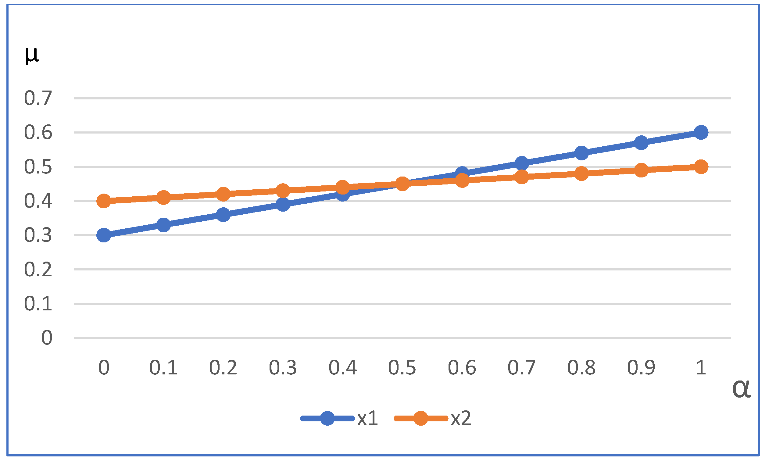
The result of Example 2 shows that when the conversion probability $\alpha$ takes different values, completely different comparison results may be obtained. We can further draw the variation trend of DM of $x_1$ and $x_2$ after conversion with conversion probability $\alpha$ through Figure 2. Since the probability conversion formula is linear, the conversion DM of $x_1$ and $x_2$ also follows a linear trend. The conversion DM of $x_1$ and $x_2$ increases with the increase of $\alpha$, which is monotonous. The relative comparison of conversion DM between $x_1$ and $x_2$ with 0.5 as the dividing line, when $\alpha <0.5$, there is $N_{\alpha }(x_1)<N_{\alpha }(x_2)$, when $\alpha >0.5$, there is $N_{\alpha }(x_1)>N_{\alpha }(x_2)$, if and only if $\alpha =0.5$, there is $N_{\alpha }(x_1)=N_{\alpha }(x_2)$.

In view of this, we cannot artificially give the conversion probability, because it is difficult to give itself; in addition, for different IFNs, the conversion probability does not have to be the same. Therefore, the comparison of IFNs cannot be made simply using a given conversion probability. However, probability conversion still provides an effective idea for the comparison of IFNs. In practice, we can compare and analyze all possible conversion cases with an “exhaustive method”, and finally, give a reasonable conclusion for the comparison of IFNs in the form of probability.

Definition 5.

Let  $x=({\mu }_1,{\nu }_1)$ and $y=({\mu }_2,{\nu }_2)$ be two IFNs, ${\pi }_1=1-{\mu }_1-{\nu }_1$, ${\pi }_2=1-{\mu }_2-{\nu }_2$, denoting $L(x)=[{\mu }_1,{\mu }_1+{\pi }_1]$ and $L(y)=[{\mu }_2,{\mu }_2+{\pi }_2]$ as the DM conversion interval of IFNs $x$ and $y$, then the dominance degree of $x$ relative to $y$ can be formalized as $P(x\ge y)={\displaystyle \underset{G}{\iint }f(m,n)dmdn}$, Where $f(m,n)$ is the joint probability density of random variables $X$ and $Y$, the value range of $X$ corresponds to $L(x)=[{\mu }_1,{\mu }_1+{\pi }_1]$, and the value range of $Y$ corresponds to $L(y)=[{\mu }_2,{\mu }_2+{\pi }_2]$. $G$ is the integral region for comparing $x\ge y$ constructed via DM conversion interval $L(x)$ and $L(y)$ of IFNs $x$ and $y$, namely $G=\{(m,n)|m\in L(x),n\in L(y),m\ge n\}$.

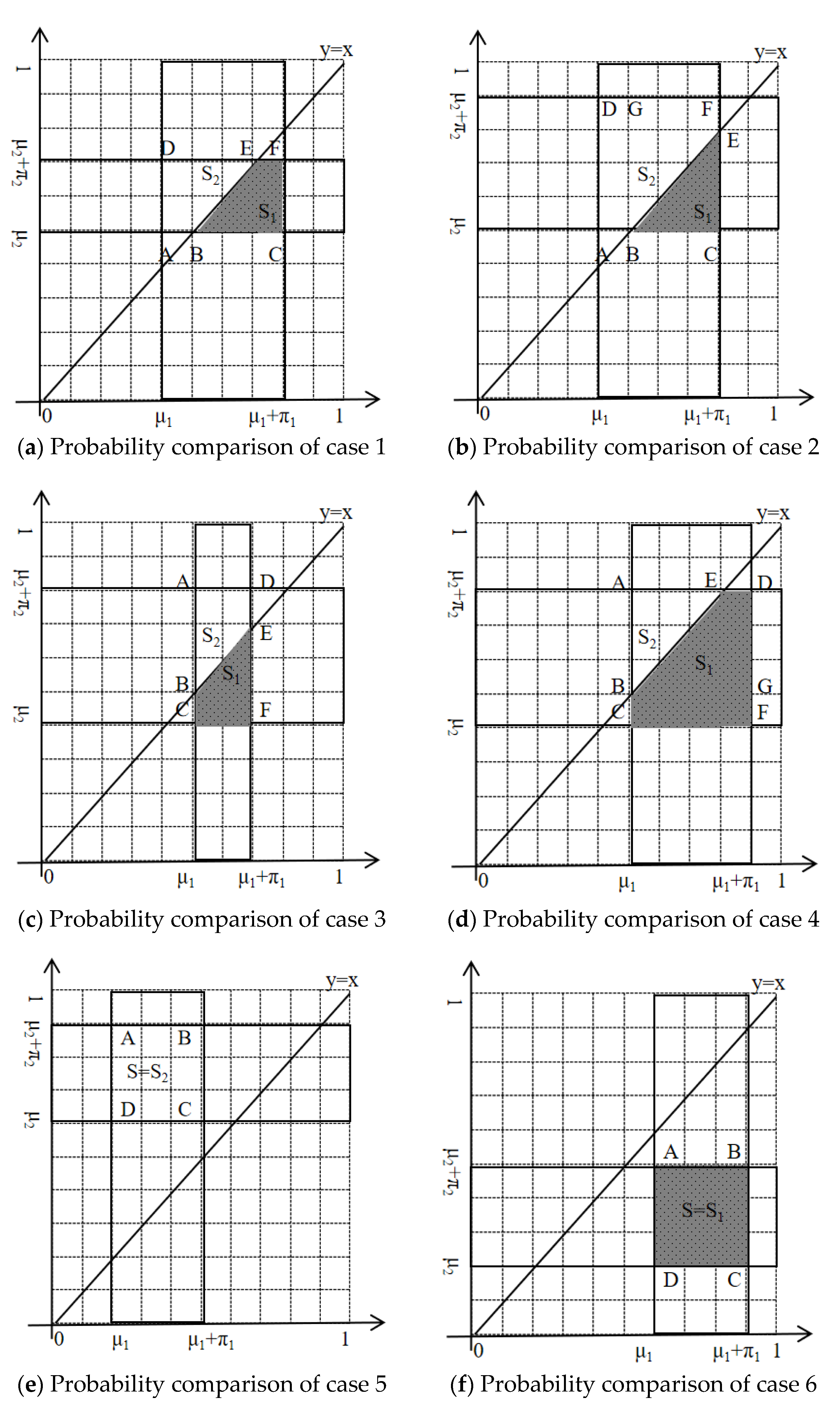
The specific expression of $P(x\ge y)$ in Definition 5 explicitly depends on the relative size relationship between ${\mu }_1,{\mu }_2,{\pi }_1,{\pi }_2$, which can be discussed in 6 cases as follows:

Case 1: ${\mu }_1\le {\mu }_2\le {\mu }_2+{\pi }_2\le {\mu }_1+{\pi }_1$; currently, the position relationship is shown in Figure 3a. The rectangular ACFD is divided into two parts via the first quadrant diagonal $y=x$. The area of the trapezoid EFCB in the lower right corner is denoted as $S_1$, and the area of the trapezoid ABED in the upper left corner is denoted as $S_2$, then $P(x\ge y)=S_1/S$, $P(x\le y)=S_2/S$.

As shown in Figure 3a, $AC={\pi }_1$, $AD={\pi }_2$, so $S={\pi }_1{\pi }_2$. Then $EF=({\mu }_1+{\pi }_1)-({\mu }_2+{\pi }_2)$, $BC=({\mu }_1+{\pi }_1)-{\mu }_2$, $CF={\pi }_2$, so $S_1=\frac{1}{2}(EF+BC)CF=\frac{{\pi }_2}{2}(2{\mu }_1+2{\pi }_1-2{\mu }_2-{\pi }_2)$. $AB={\mu }_2-{\mu }_1$, $DE={\mu }_2+{\pi }_2-{\mu }_1$, $AD={\pi }_2$, then $S_2=\frac{1}{2}(AB+DE)AD=\frac{{\pi }_2}{2}(2{\mu }_2-2{\mu }_1+{\pi }_2)$. There is:

$P(x\ge y)=\frac{S_1}{S}=\frac{2{\mu }_1+2{\pi }_1-2{\mu }_2-{\pi }_2}{2{\pi }_1}$, $P(x\le y)=\frac{S_2}{S}=\frac{2{\mu }_2-2{\mu }_1+{\pi }_2}{2{\pi }_1}$, it is easy to verify $S_1+S_2=S$, $P(x\ge y)+P(x\le y)=1$.

Case 2: ${\mu }_1\le {\mu }_2\le {\mu }_1+{\pi }_1\le {\mu }_2+{\pi }_2$, the position relationship is shown in Figure 3b, and the other symbol marks and interpretation are the same as Case 1.

As shown in Figure 3b, $AC={\pi }_1$, $AD={\pi }_2$, so $S={\pi }_1{\pi }_2$. Because $BC=CF={\mu }_1+{\pi }_1-{\mu }_2$, there is $S_1=\frac{1}{2}{({\mu }_1+{\pi }_1-{\mu }_2)}^2$. The calculation of $S_2$ needs to divide the pentagon ABEFD into rectangular ABGD and trapezoidal EFGB, and $AB={\mu }_2-{\mu }_1$, $AD={\pi }_2$, so $S_{ABGD}=({\mu }_2-{\mu }_1){\pi }_2$. Because $EF=({\mu }_2+{\pi }_2)-({\mu }_1+{\pi }_1)$, $BG={\pi }_2$, $GF={\mu }_1+{\pi }_1-{\mu }_2$, so $S_{EFGB}=\frac{1}{2}({\mu }_2+2{\pi }_2-{\mu }_1-{\pi }_1)({\mu }_1+{\pi }_1-{\mu }_2)$, then $S_2=S_{ABGD}+S_{EFGB}$$=\frac{1}{2}[2{\pi }_1({\mu }_2-{\mu }_1)+{\pi }_1(2{\pi }_2-{\pi }_1)-{({\mu }_2-{\mu }_1)}^2]$. Thus,

$$P(x\ge y)=\frac{S_1}{S}=\frac{{({\mu }_1+{\pi }_1-{\mu }_2)}^2}{2{\pi }_1{\pi }_2},P(x\le y)=\frac{S_2}{S}=\frac{2{\pi }_1({\mu }_2-{\mu }_1)+{\pi }_1(2{\pi }_2-{\pi }_1)-{({\mu }_2-{\mu }_1)}^2}{2{\pi }_1{\pi }_2}.$$

Case 3: ${\mu }_2\le {\mu }_1\le {\mu }_1+{\pi }_1\le {\mu }_2+{\pi }_2$, and the position relationship is shown in Figure 3c.

As shown in Figure 3c, $AC={\pi }_1$, $AD={\pi }_2$, so $S={\pi }_1{\pi }_2$. Because $CB={\mu }_1-{\mu }_2$, $FE={\mu }_1+{\pi }_1-{\mu }_2$, $CF={\pi }_1$, so $S_1=\frac{1}{2}(CB+FE)CF=\frac{{\pi }_1}{2}(2{\mu }_1-2{\mu }_2+{\pi }_1)$. With $DE=({\mu }_2+{\pi }_2)-({\mu }_1+{\pi }_1)$, $AB={\mu }_2+{\pi }_2-{\mu }_1$, $AD={\pi }_1$, then $S_2=\frac{1}{2}(DE+AB)AD=\frac{{\pi }_1}{2}(2{\mu }_2+2{\pi }_2-2{\mu }_1-{\pi }_1)$. Hence,

$$P(x\ge y)=\frac{S_1}{S}=\frac{2{\mu }_1-2{\mu }_2+{\pi }_1}{2{\pi }_2},P(x\le y)=\frac{S_2}{S}=\frac{2{\mu }_2+2{\pi }_2-2{\mu }_1-{\pi }_1}{2{\pi }_2}.$$

Case 4: ${\mu }_2\le {\mu }_1\le {\mu }_2+{\pi }_2\le {\mu }_1+{\pi }_1$, and the position relationship is shown in Figure 3d.

As shown in Figure 3d, $AC={\pi }_1$, $AD={\pi }_2$, so $S={\pi }_1{\pi }_2$. The calculation of $S_1$ needs to divide the pentagonal BCFDE into rectangular BCFG and trapezoidal EDGB, and $BC={\mu }_1-{\mu }_2$, $CF={\pi }_1$, so $S_{BCGF}=({\mu }_1-{\mu }_2){\pi }_1$. Because $ED=({\mu }_1+{\pi }_1)-({\mu }_2+{\pi }_2)$, $BG={\pi }_1$, $DG={\mu }_2+{\pi }_2-{\mu }_1$, so $S_{EDGB}=$$\frac{1}{2}({\mu }_1+2{\pi }_1-{\mu }_2-{\pi }_2)({\mu }_2+{\pi }_2-{\mu }_1)$, $S_1=S_{BCGF}+S_{EDGB}=\frac{1}{2}[2{\pi }_2({\mu }_1-{\mu }_2)+{\pi }_2(2{\pi }_1-{\pi }_2)-{({\mu }_1-{\mu }_2)}^2]$. $AB=AE={\mu }_2+{\pi }_2-{\mu }_1$, $S_2=\frac{1}{2}{({\mu }_2+{\pi }_2-{\mu }_1)}^2$. Hence,

$$P(x\ge y)=\frac{S_1}{S}=\frac{2{\pi }_2({\mu }_1-{\mu }_2)+{\pi }_2(2{\pi }_1-{\pi }_2)-{({\mu }_1-{\mu }_2)}^2}{2{\pi }_1{\pi }_2},P(x\le y)=\frac{S_2}{S}=\frac{{({\mu }_2+{\pi }_2-{\mu }_1)}^2}{2{\pi }_1{\pi }_2}.$$

Case 5: ${\mu }_1\le {\mu }_1+{\pi }_1\le {\mu }_2\le {\mu }_2+{\pi }_2$, the position relationship is shown in Figure 3e. Obviously, $S_1=0$, $S_2=S={\pi }_1{\pi }_2$, i.e., $P(x\ge y)=0$, $P(x\le y)=1$.

Case 6: ${\mu }_2\le {\mu }_2+{\pi }_2\le {\mu }_1\le {\mu }_1+{\pi }_1$, the position relationship is shown in Figure 3f. Obviously, $S_2=0$, $S_1=S={\pi }_1{\pi }_2$, i.e., $P(x\ge y)=1$, $P(x\le y)=0$.

By summarizing the above 6 cases, we can obtain:

$$\begin{array}{c}P(x\ge y)=\left\{\begin{array}{l}\frac{2{\mu }_1+2{\pi }_1-2{\mu }_2-{\pi }_2}{2{\pi }_1},{\mu }_1\le {\mu }_2\le {\mu }_2+{\pi }_2\le {\mu }_1+{\pi }_1\\ \frac{{({\mu }_1+{\pi }_1-{\mu }_2)}^2}{2{\pi }_1{\pi }_2},{\mu }_1\le {\mu }_2\le {\mu }_1+{\pi }_1\le {\mu }_2+{\pi }_2\\ \frac{2{\mu }_1-2{\mu }_2+{\pi }_1}{2{\pi }_2},{\mu }_2\le {\mu }_1\le {\mu }_1+{\pi }_1\le {\mu }_2+{\pi }_2\\ \frac{2{\pi }_2({\mu }_1-{\mu }_2)+{\pi }_2(2{\pi }_1-{\pi }_2)-{({\mu }_1-{\mu }_2)}^2}{2{\pi }_1{\pi }_2},{\mu }_2\le {\mu }_1\le {\mu }_2+{\pi }_2\le {\mu }_1+{\pi }_1\\ 0,{\mu }_1\le {\mu }_1+{\pi }_1\le {\mu }_2\le {\mu }_2+{\pi }_2\\ 1,{\mu }_2\le {\mu }_2+{\pi }_2\le {\mu }_1\le {\mu }_1+{\pi }_1\end{array}\right.\\ P(x\le y)=\left\{\begin{array}{l}\frac{2{\mu }_2-2{\mu }_1+{\pi }_2}{2{\pi }_1},{\mu }_1\le {\mu }_2\le {\mu }_2+{\pi }_2\le {\mu }_1+{\pi }_1\\ \frac{2{\pi }_1({\mu }_2-{\mu }_1)+{\pi }_1(2{\pi }_2-{\pi }_1)-{({\mu }_2-{\mu }_1)}^2}{2{\pi }_1{\pi }_2},{\mu }_1\le {\mu }_2\le {\mu }_1+{\pi }_1\le {\mu }_2+{\pi }_2\\ \frac{2{\mu }_2+2{\pi }_2-2{\mu }_1-{\pi }_1}{2{\pi }_2},{\mu }_2\le {\mu }_1\le {\mu }_1+{\pi }_1\le {\mu }_2+{\pi }_2\\ \frac{{({\mu }_2+{\pi }_2-{\mu }_1)}^2}{2{\pi }_1{\pi }_2},{\mu }_2\le {\mu }_1\le {\mu }_2+{\pi }_2\le {\mu }_1+{\pi }_1\\ 1,{\mu }_1\le {\mu }_1+{\pi }_1\le {\mu }_2\le {\mu }_2+{\pi }_2\\ 0,{\mu }_2\le {\mu }_2+{\pi }_2\le {\mu }_1\le {\mu }_1+{\pi }_1\end{array}\right.\end{array}.$$

From the above 6 cases, it is not difficult to see that case 3 has a “symmetric” relationship with case 1, case 4 has a “symmetric” relationship with case 2, and case 6 has a “symmetric” relationship with case 5. The concrete embodiment of this “symmetric” relationship is as follows: first, the position is symmetric about $y=x$, and second, the probability value of comparison is symmetric and complementary.

In fact, according to the solution formula in 6 cases above, we can define the formal integral of probability comparison in Definition 5 as follows:

$$P(x\ge y)={\displaystyle {\int }_{\max ({\mu }_1,{\mu }_2)}^{{\mu }_1+{\pi }_1}dm}{\displaystyle {\int }_{{\mu }_2}^{\min (x,{\mu }_2+{\pi }_2)}\frac{1}{{\pi }_1{\pi }_2}dn}$$

where $f(m,n)=\frac{1}{{\pi }_1{\pi }_2}$ is the joint probability density of random variables $X$ and $Y$ under uniform distribution. Taking case 1 as an example, the above equation $P(x\ge y)$ can be concretized as follows:

$$\begin{array}{l}P(x\ge y)={\displaystyle {\int }_{\max ({\mu }_1,{\mu }_2)}^{{\mu }_1+{\pi }_1}dm}{\displaystyle {\int }_{{\mu }_2}^{\min (x,{\mu }_2+{\pi }_2)}\frac{1}{{\pi }_1{\pi }_2}dn}={\displaystyle {\int }_{{\mu }_2}^{{\mu }_2+{\pi }_2}dm}{\displaystyle {\int }_{{\mu }_2}^x\frac{1}{{\pi }_1{\pi }_2}dn}+{\displaystyle {\int }_{{\mu }_2+{\pi }_2}^{{\mu }_1+{\pi }_1}dm}{\displaystyle {\int }_{{\mu }_2}^{{\mu }_2+{\pi }_2}\frac{1}{{\pi }_1{\pi }_2}dn}\\ =\frac{1}{{\pi }_1{\pi }_2}\left({\displaystyle {\int }_{{\mu }_2}^{{\mu }_2+{\pi }_2}(x-{\mu }_2)dm}+{\displaystyle {\int }_{{\mu }_2+{\pi }_2}^{{\mu }_1+{\pi }_1}{\pi }_{2}dm}\right)=\frac{1}{{\pi }_1{\pi }_2}\left({\displaystyle {\int }_{{\mu }_2}^{{\mu }_2+{\pi }_2}(x-{\mu }_2)dm}+{\displaystyle {\int }_{{\mu }_2+{\pi }_2}^{{\mu }_1+{\pi }_1}{\pi }_{2}dm}\right)\\ =\frac{1}{{\pi }_1{\pi }_2}\left({\left.\left(\frac{x^2}{2}-{\mu }_{2}x\right)\right|}_{{\mu }_2}^{{\mu }_2+{\pi }_2}+{\pi }_2{\left.m\right|}_{{\mu }_2+{\pi }_2}^{{\mu }_1+{\pi }_1}\right)=\frac{1}{{\pi }_1{\pi }_2}\left({\left.\left(\frac{x^2}{2}-{\mu }_{2}x\right)\right|}_{{\mu }_2}^{{\mu }_2+{\pi }_2}+{\pi }_2{\left.m\right|}_{{\mu }_2+{\pi }_2}^{{\mu }_1+{\pi }_1}\right)\\ =\frac{1}{{\pi }_1{\pi }_2}\left(\frac{{\pi }_{{}_2}^2}{2}+{\pi }_2({\mu }_1+{\pi }_1-{\mu }_2-{\pi }_2)\right)=\frac{(2{\mu }_1+2{\pi }_1-2{\mu }_2-{\pi }_2)}{2{\pi }_1}\end{array}$$

The calculation results are completely consistent with case 1 in Definition 5, and the remaining five cases can be solved in the form of integrals in the same way. Limited by space, we will not repeat them here.

Property 1.

Let $x=({\mu }_x,{\nu }_x)$, $y=({\mu }_y,{\nu }_y)$ and $z=({\mu }_z,{\nu }_z)$ be any three IFNs, then:

(1)

$0\le P(x\ge y)\le 1$;

(2)

$P(x\ge y)+P(y\ge x)=1$;

(3)

$P(x\ge x)=0.5$;

(4)

$P(x\ge y)=0$ if $1-{\nu }_x\le {\mu }_y$;

(5)

$P(x\ge y)=1$ if $1-{\nu }_y\le {\mu }_x$;

(6)

$P(x\ge y)=0.5$ if ${\mu }_x-{\nu }_x={\mu }_y-{\nu }_y$;

(7)

$P(x\ge y)\ge 0.5$ if ${\mu }_x-{\nu }_x\ge {\mu }_y-{\nu }_y$;

(8)

if $P(x\ge y)=0$, $P(y\ge z)=0$, then $P(x\ge z)=0$;

(9)

if $P(x\ge y)=1$, $P(y\ge z)=1$, then $P(x\ge z)=1$;

(10)

if $P(x\ge y)\ge 0.5$, $P(y\ge z)\ge 0.5$, then $P(x\ge z)\ge 0.5$.

Proof. 

Properties (1) and (2) are obviously true from the six cases in the above equation.

(3) On the one hand, let $y=x$, then there is ${\mu }_y={\mu }_x$, ${\nu }_y={\nu }_x$, ${\pi }_y={\pi }_x$. Substituting ${\mu }_y={\mu }_x$ and ${\pi }_y={\pi }_x$ into case 1 to case 4 in the above formula, the conclusion of $P(x\ge x)=0.5$ can be obtained. On the other hand, according to property (2), let $y=x$, there is also $P(x\ge x)+P(x\ge x)=1$, i.e., $P(x\ge x)=0.5$.

(4) Adequacy: if $P(x\ge y)=0$, it conforms to case 5, i.e., ${\mu }_x+{\pi }_x\le {\mu }_y$, since ${\mu }_x+{\pi }_x=1-{\nu }_x$, so $1-{\nu }_x\le {\mu }_y$. Necessity: If $1-{\nu }_x\le {\mu }_y$, then there is ${\mu }_x+{\pi }_x\le {\mu }_y$, which obviously conforms to case 5, then $P(x\ge y)=0$ can be obtained.

(5) Adequacy: if $P(x\ge y)=1$, it conforms to case 6, that is ${\mu }_y+{\pi }_y\le {\mu }_x$. Because of ${\mu }_y+{\pi }_y=1-{\nu }_y$, there is $1-{\nu }_y\le {\mu }_x$. Necessity can also be proved; this is omitted.

(6) Adequacy: if $P(x\ge y)=0.5$, it corresponds to part of cases 1 and 3. In case 1, it is satisfied that AB = EF, where, $AB={\mu }_y-{\mu }_x$, $EF=({\mu }_x+{\pi }_x)-({\mu }_y+{\pi }_y)$, and then there is ${\mu }_y-{\mu }_x=({\mu }_x+{\pi }_x)-({\mu }_y+{\pi }_y)$, that is ${\mu }_y-{\mu }_x=(1-{\nu }_x)-(1-{\nu }_y)$, i.e., ${\mu }_x-{\nu }_x={\mu }_y-{\nu }_y$. In case 3, BC = DE, with $BC={\mu }_x-{\mu }_y$, $DE=({\mu }_y+{\pi }_y)-({\mu }_x+{\pi }_x)$, we have ${\mu }_x-{\mu }_y=({\mu }_y+{\pi }_y)-({\mu }_x+{\pi }_x)$, that is ${\mu }_x-{\mu }_y=(1-{\nu }_y)-(1-{\nu }_x)$, i.e., ${\mu }_x-{\nu }_x={\mu }_y-{\nu }_y$. Necessity can also be proved; this is omitted.

(7) Adequacy: It can be further verified on the basis of property (6). In case 1, if AB ≤ EF is satisfied, there is ${\mu }_y-{\mu }_x\le ({\mu }_x+{\pi }_x)-({\mu }_y+{\pi }_y)$, and ${\mu }_x-{\nu }_x\ge {\mu }_y-{\nu }_y$ can be obtained via simplification. In case 3, if BC ≥ DE is satisfied, then we have ${\mu }_x-{\mu }_y\ge ({\mu }_y+{\pi }_y)-({\mu }_x+{\pi }_x)$, which is simplified to ${\mu }_x-{\nu }_x\ge {\mu }_y-{\nu }_y$. Necessity can also be proved; this is omitted.

(8) According to property (4), if $P(x\ge y)=0$, then $1-{\nu }_x\le {\mu }_y$, and if $P(y\ge z)=0$, then $1-{\nu }_y\le {\mu }_z$. Obviously, $1-{\nu }_y={\mu }_y+{\pi }_y\ge {\mu }_y$, which is $1-{\nu }_x\le {\mu }_y\le 1-{\nu }_y\le {\mu }_z$; then, we have $1-{\nu }_x\le {\mu }_z$, so $P(x\ge z)=0$ is true.

(9) According to property (5), if $P(x\ge y)=1$, then $1-{\nu }_y\le {\mu }_x$, and if $P(y\ge z)=1$, then $1-{\nu }_z\le {\mu }_y$. Obviously, $1-{\nu }_y={\mu }_y+{\pi }_y\ge {\mu }_y$, which is $1-{\nu }_z\le {\mu }_y\le 1-{\nu }_y\le {\mu }_x$; then, we have $1-{\nu }_z\le {\mu }_x$, so $P(x\ge z)=1$ is true.

(10) According to property (7), if $P(x\ge y)\ge 0.5$, then ${\mu }_x-{\nu }_x\ge {\mu }_y-{\nu }_y$, and if $P(y\ge z)\ge 0.5$, then ${\mu }_y-{\nu }_y\ge {\mu }_z-{\nu }_z$. Obviously, ${\mu }_x-{\nu }_x\ge {\mu }_y-{\nu }_y\ge {\mu }_z-{\nu }_z$, so $P(x\ge z)\ge 0.5$ is true. □

Definition 6.

Let  $U=\{x_1,x_2,\dots ,x_n|x_i=({\mu }_i,{\nu }_i)\}$ be a set of the universe containing $n$ IFNs. For $\forall x_i,x_j\in U$, let $p_{ij}=P(x_i\ge x_j)$ represent the dominance degree of $x_i$ relative to $x_j$, then $P={[p_{ij}]}_{n\times n}$ represents the dominance matrix on $U$, and further define the comprehensive dominance degree of each object as $D={(d_1,d_2,\dots ,d_n)}^T$, where $d_i=\frac{1}{n}{\displaystyle \sum _{j=1}^n{p}_{ij}}(i=1,2,\dots n)$.

The IFNs on $U$ can be sorted and compared according to the value of $D$.

4. Intuitionistic Fuzzy Probability Dominance Relation and Multi-Attribute Decision-Making

Definition 7.

We call  $IS=\{U,B,V,f\}$ an intuitionistic fuzzy information system (IFIS), where $U=\{x_1,x_2,\dots ,x_n\}$ is the non-empty finite universe, $B=\{b_1,b_2,\dots ,b_m\}$ is the non-empty finite attribute set, $f:U\times B\to V$, that is $\forall b\in B,x\in U$, $f(x,b)\in V$ is a IFN, $V$ is the intuitionistic fuzzy set of different objects under different attributes, and $V_a$ is a partial order set under attribute $a\in B$.

Definition 8.

Let  $IS=\{U,B,V,f\}$ be the IFIS, for  $\forall x_i,x_j\in U$,$b\in B$, denote

$${\lambda }_{{}_b}^{\alpha }(x_i,x_j)=\left\{\begin{array}{l}1,\hspace{0.33em}{p}_{ij}^b=P(f(x_i,b)\ge f(x_j,b))\ge \alpha \\ 0,\hspace{0.33em}{p}_{ij}^b=P(f(x_i,b)\ge f(x_j,b))<\alpha \end{array}\right.$$

as the binary judgment of the $\alpha$ probability dominance value of object $x_i$ relative to $x_j$ under attribute $b$; furthermore, let ${\lambda }_{{}_B}^{\alpha }(x_i,x_j)={\displaystyle \sum _{b\in B}{\lambda }_{{}_b}^{\alpha }(x_i,x_j)}/|B|$, and the intuitionistic fuzzy probability dominance relation (IFPDR) of $U$ on $B$ is defined as $R_B^{\ge (\alpha ,\beta )}=\{(x_i,x_j)\in U\times U|{\lambda }_{{}_B}^{\alpha }(x_i,x_j)\ge \beta \}$, where $\left|B\right|$ represents the number of attribute sets, $\alpha$ and $\beta$ are the threshold of IFPDR, generally $0.5\le \alpha \le 1$, $0.5\le \beta \le 1$.

Based on IFPDR, we can define the intuitionistic fuzzy probability dominance class of object $x_i$ under attribute sets $B$ as ${[x_i]}_B^{\ge (\alpha ,\beta )}=\left\{x_j\right|(x_i,x_j)\in R_B^{\ge (\alpha ,\beta )}\}$. For $\forall x_j\in {[x_i]}_B^{\ge (\alpha ,\beta )}$, its meaning is based on the probabilistic dominance comparison rule of IFNs. Under all attributes, $x_i$ is superior to $x_j$ with a probability of no less than $\alpha$ and the attribute proportion is no less than $\beta$. Similarly, the intuitionistic fuzzy probability inferiority class of object $x_i$ under attribute sets $B$ can be defined as ${[x_i]}_B^{\le (\alpha ,\beta )}=\left\{x_j\right|(x_j,x_i)\in R_B^{\ge (\alpha ,\beta )}\}$.

Taking $\alpha$ and $\beta$ as thresholds to define the IFPDR, the main starting point is based on the consideration of practical problems. In the realistic MADM, it is difficult to make objects meet the strict superiority and inferiority relationship under all attributes, and too strict parameter setting often leads to the decision failure. Therefore, relaxing the comparison requirement between objects is more helpful to obtain reasonable results for MADM problems.

In particular, when $\beta =1$, it is required that the relationship of probabilistic superiority or probabilistic inferiority between objects is satisfied under all attributes; when $\alpha =1$, it is required that the IFNs themselves have an absolute relationship between superiority or inferiority; when $\alpha =\beta =1$, it means that the object represented by IFNs has an absolute relationship between superiority or inferiority under all attributes, which is difficult to satisfy in MADM. Therefore, by introducing parameters $\alpha$ and $\beta$ as the decision threshold, decision-makers can adjust the threshold according to the actual situation in practical problems. According to the “half rule”, $\alpha$ and $\beta$ should not be lower than 0.5.

Property 2.

Let $IS=\{U,B,V,f\}$ be an IFIS. For $\forall x_i\in U$, $0.5\le {\alpha }_1\le {\alpha }_2\le \alpha \le 1$, $0.5\le {\beta }_1\le {\beta }_2\le \beta \le 1$, there is:

(1)

$R_B^{\ge ({\alpha }_2,\beta )}\subseteq R_B^{\ge ({\alpha }_{{}_1},\beta )}$;

(2)

$R_B^{\ge (\alpha ,{\beta }_2)}\subseteq R_B^{\ge (\alpha ,{\beta }_1)}$;

(3)

${[x_i]}_B^{\ge ({\alpha }_2,\beta )}\subseteq {[x_i]}_B^{\ge ({\alpha }_1,\beta )}$;

(4)

${[x_i]}_B^{\ge (\alpha ,{\beta }_2)}\subseteq {[x_i]}_B^{\ge (\alpha ,{\beta }_1)}$.

The proof of property is obvious and omitted here.

Definition 9.

Let  $IS=\{U,B,V,f\}$ be the  IFIS,  $R_B^{\ge (\alpha ,\beta )}$  is the  IFPDR of  $U$ on $B$, then  $M_B^{\ge (\alpha ,\beta )}$  is the intuitionistic fuzzy probability dominance intercept matrix of  $U$  on  $B$, where the corresponding relation between  $M_B^{\ge (\alpha ,\beta )}$  and  $R_B^{\ge (\alpha ,\beta )}$  is: 

$$M_B^{\ge (\alpha ,\beta )}=\{{[m_{ij}]}_{n\times n}|m_{ij}=\left\{\begin{array}{l}1,(x_i,x_j)\in R_B^{\ge (\alpha ,\beta )}\\ 0,(x_i,x_j)\notin R_B^{\ge (\alpha ,\beta )}\end{array}\right.\}$$

Definition 10.

Let  $IS=\{U,B,V,f\}$ be the IFIS, $M_B^{\ge (\alpha ,\beta )}$ is the intuitionistic fuzzy probability dominance intercept matrix of $U$ on $B$, $C_B^{\ge (\alpha ,\beta )}={[c_{ij}]}_{n\times n}=M_B^{\ge (\alpha ,\beta )}\cdot M_B^{\ge (\alpha ,\beta )}$ is the intuitionistic fuzzy probability dominance matrix of $U$ on $B$, and $c_i=\frac{1}{n}{\displaystyle \sum _{j=1}^n{c}_{ij}}(i=1,2,\dots n)$ be the average dominance degree of object $x_i$.

The above definition of the dominance matrix is equivalent to $c_{ij}=|{[x_i]}_B^{\ge (\alpha ,\beta )}\cap {[x_j]}_B^{\le (\alpha ,\beta )}|$, that is, the intersection of the object set dominated by $x_i$ and the object set not inferior to $x_j$ is taken as a measure of the degree to which $x_i$ is superior to $x_j$. In MADM, all objects can be sorted according to the value of $c_i$.

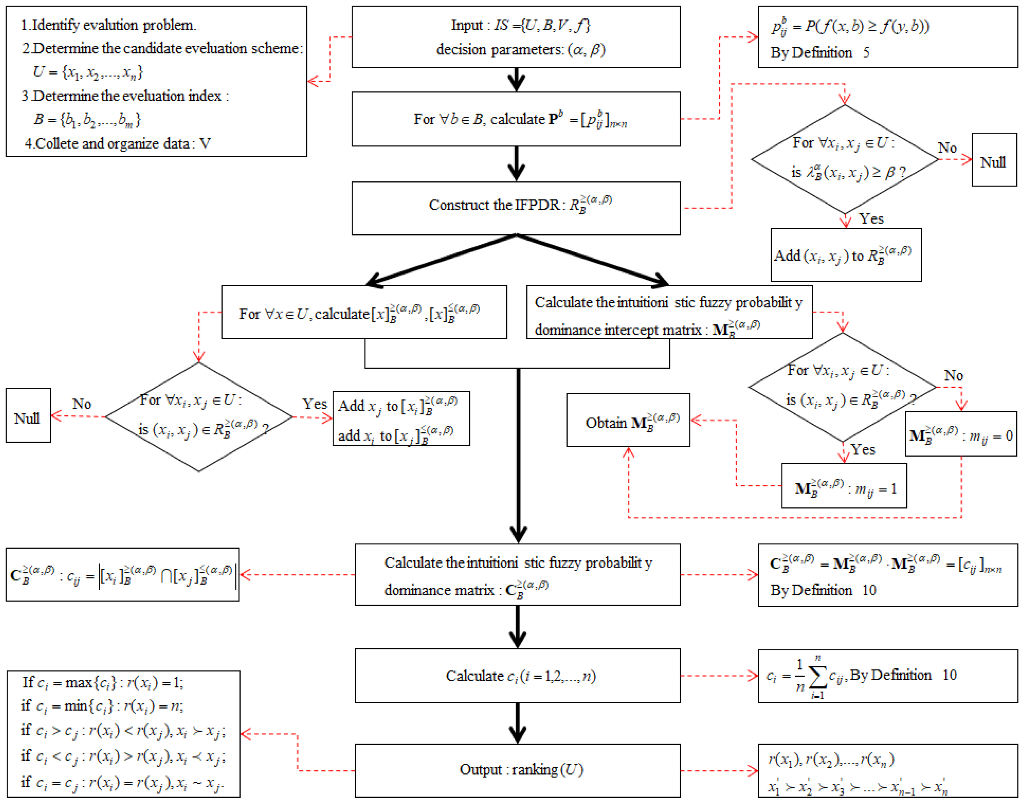
Combined with the above analysis, the steps of this paper’s probability dominance relation for MADM based on IFNs can be summarized as follows (as shown in Figure 4):

Step 1: For $\forall b\in B$, calculate the dominance degree $P^b={[p_{ij}^b]}_{n\times n}$ of pairwise comparison of objects in domain $U$;

Step 2: Construct the IFPDR $R_B^{\ge (\alpha ,\beta )}$ and intuitionistic fuzzy probability dominance intercept matrix $M_B^{\ge (\alpha ,\beta )}$ according to $P^b$;

Step 3: Calculate the intuitionistic fuzzy probability dominance matrix $C_B^{\ge (\alpha ,\beta )}$ according to $M_B^{\ge (\alpha ,\beta )}$;

Step 4: Calculate the average dominance degree $c_i$ according to $C_B^{\ge (\alpha ,\beta )}$, and sort the objects and schemes according to the value of $c_i$.

5. Case Application and Analysis

With the rapid development of social economy, e-commerce has gradually become a new industry and a link between commodities and consumers all over the world. Online shopping has also increasingly become a new consumption mode for contemporary young people and is becoming increasingly popular. In particular, the prevalence of COVID-19 between 2019 and 2022 has further promoted the development of e-commerce. In online shopping choices, logistics and distribution problems often become the key factors for consumers to choose whether to buy or not. After all, we do not want to have the situation that there is no delivery a week after we place an order, or the embarrassment caused by the logistics delay that makes the online gift miss a friend’s birthday. Therefore, the quality of logistics services largely determines whether a region or consumer group chooses online consumption.

In order to evaluate the service quality of express delivery points in a university and provide reference for them to improve the service quality, we designed the corresponding questionnaire. Through field visits and observation, we found that there are altogether 10 express delivery companies settled in M university with branches. They are SF Express, YTO Express, ZTO Express, STO Express, Best Express, TTK Express, Yunda, CPEL, JD Express, and Jitu Express. Therefore, we took the service branches of these 10 express delivery companies as the investigation objects. The evaluation indexes of logistics service quality are obtained by referring to relevant literature, consulting experts in the field and communicating with teachers and students of M university. Finally, through discussion and screening, nine factors are determined as the evaluation indexes of logistics service quality. They are price, delivery speed, service attitude, service professionalism, timeliness of logistics information update, rationality of delivery time, integrity of products and packaging, remedial measures taken for service errors, and popularity of express companies. When constructing the information table, we mark the 10 service outlets of express enterprises to be evaluated as $U=\{x_1,x_2,\dots ,x_{10}\}$, and the 9 evaluation indexes affecting the quality of logistics service as $B=\{b_1,b_2,\dots ,b_9\}$.

In order to construct the data table in line with the form of IFNs as objectively as possible, when assigning values to the indexes of each express company, the questionnaire only sets three options for the attribute value of each index $b_j$, which are respectively “good”, “poor” and “unclear”. If the respondents approve the performance of a courier company under this index, they choose “good”; if the respondents do not approve the performance of a courier company under this index, they choose “bad”; in particular, if the respondents have not used the relevant services of a courier company, or do not have a deep impression and understanding of a courier company so that it is difficult to judge, they can choose “unclear”.

Based on the above survey objectives and questionnaire design, a questionnaire was issued to teachers and students of M university to solve this problem. The questionnaire was made through the network and released through social software in December 2022. A total of 508 valid samples were collected. According to the number of respondents for each option, the proportions of “good”, “bad”, and “unclear” were calculated as the DM, DN, and DH of the IFNs, and the original data information table is shown in

Table 1. Original data of express delivery evaluation in M university.

U/B	b1	b2	b3	b4	b5	b6	b7	b8	b9
x1	(0.69, 0.09)	(0.67, 0.07)	(0.54, 0.12)	(0.73, 0.15)	(0.76, 0.13)	(0.47, 0.13)	(0.65, 0.10)	(0.51, 0.13)	(0.51, 0.13)
x2	(0.51, 0.19)	(0.57, 0.16)	(0.65, 0.17)	(0.39, 0.10)	(0.50, 0.16)	(0.46, 0.13)	(0.63, 0.10)	(0.31, 0.10)	(0.31, 0.10)
x3	(0.32, 0.22)	(0.37, 0.22)	(0.35, 0.21)	(0.51, 0.11)	(0.43, 0.19)	(0.41, 0.10)	(0.55, 0.21)	(0.43, 0.23)	(0.43, 0.23)
x4	(0.33, 0.22)	(0.30, 0.24)	(0.51, 0.22)	(0.32, 0.22)	(0.38, 0.23)	(0.42, 0.20)	(0.52, 0.23)	(0.43, 0.25)	(0.43, 0.25)
x5	(0.22, 0.16)	(0.30, 0.45)	(0.34, 0.22)	(0.26, 0.12)	(0.43, 0.29)	(0.36, 0.16)	(0.35, 0.27)	(0.27, 0.30)	(0.27, 0.30)
x6	(0.30, 0.31)	(0.20, 0.38)	(0.31, 0.10)	(0.40, 0.27)	(0.30, 0.25)	(0.50, 0.15)	(0.40, 0.23)	(0.39, 0.27)	(0.39, 0.27)
x7	(0.33, 0.25)	(0.46, 0.13)	(0.55, 0.20)	(0.49, 0.19)	(0.55, 0.11)	(0.37, 0.20)	(0.55, 0.23)	(0.43, 0.12)	(0.43, 0.12)
x8	(0.48, 0.29)	(0.24, 0.15)	(0.52, 0.22)	(0.49, 0.20)	(0.33, 0.15)	(0.56, 0.27)	(0.34, 0.10)	(0.44, 0.22)	(0.44, 0.22)
x9	(0.44, 0.10)	(0.70, 0.12)	(0.74, 0.16)	(0.45, 0.13)	(0.57, 0.13)	(0.50, 0.15)	(0.74, 0.13)	(0.38, 0.17)	(0.38, 0.17)
x10	(0.21, 0.10)	(0.23, 0.15)	(0.30, 0.20)	(0.42, 0.20)	(0.46, 0.12)	(0.48, 0.10)	(0.43, 0.24)	(0.38, 0.13)	(0.38, 0.13)

.

(1) Calculate the dominance degree under each attribute. Take $b_1$ as an example, and the results are as follows:

$$P^{b_1}=\left[\begin{array}{cccccccccc}0.5& 0.891& 0.960& 0.959& 0.918& 1& 0.981& 0.996& 0.782& 0.855\\ 0.109& 0.5& 0.736& 0.730& 0.710& 0.862& 0.771& 0.710& 0.478& 0.652\\ 0.040& 0.264& 0.5& 0.489& 0.532& 0.618& 0.522& 0.402& 0.273& 0.493\\ 0.041& 0.270& 0.511& 0.5& 0.540& 0.631& 0.533& 0.411& 0.279& 0.5\\ 0.082& 0.290& 0.468& 0.460& 0.5& 0.556& 0.484& 0.395& 0.281& 0.464\\ 0& 0.138& 0.382& 0.369& 0.444& 0.5& 0.396& 0.246& 0.174& 0.413\\ 0.019& 0.229& 0.478& 0.467& 0.516& 0.604& 0.5& 0.369& 0.249& 0.478\\ 0.004& 0.290& 0.598& 0.589& 0.605& 0.754& 0.631& 0.5& 0.337& 0.558\\ 0.218& 0.522& 0.727& 0.721& 0.719& 0.826& 0.751& 0.663& 0.5& 0.667\\ 0.145& 0.348& 0.507& 0.5& 0.536& 0.587& 0.522& 0.442& 0.333& 0.5\end{array}\right]$$

Taking the solution of $P_{12}^{b_1}=0.891$ as an example, the calculation process is briefly shown as follows:

In the attribute set of $b_1$, the values of $x_1$ and $x_2$ are $x_1=(0.69,0.09)$ and $x_2=(0.51,0.19)$ respectively (The attribute tag $b_1$ is omitted here for convenience of expression). Further calculation of its DH can be seen as follows:

$${\pi }_1=1-{\mu }_1-{\nu }_1=1-0.69-0.09=0.22,{\pi }_2=1-{\mu }_2-{\nu }_2=1-0.51-0.19=0.30.$$

Since 0.51 < 0.69 < 051 + 0.30 < 0.69 + 0.22, case 4 in Definition 5 is satisfied, namely:

$${\mu }_2\le {\mu }_1\le {\mu }_2+{\pi }_2\le {\mu }_1+{\pi }_1$$

then $P(x_1\ge x_2)$ can be calculated as follows:

$$\begin{array}{l}P(x_1\ge x_2)=\frac{2{\pi }_2({\mu }_1-{\mu }_2)+{\pi }_2(2{\pi }_1-{\pi }_2)-{({\mu }_1-{\mu }_2)}^2}{2{\pi }_1{\pi }_2}\\ =\frac{2\times 0.30\times (0.69-0.51)+0.30\times (2\times 0.22-0.30)-{(0.69-0.51)}^2}{2\times 0.22\times 0.30}\\ =\frac{0.1176}{0.132}\approx 0.891\end{array}$$

Other data in $P^{b_1}$ can be similarly obtained.

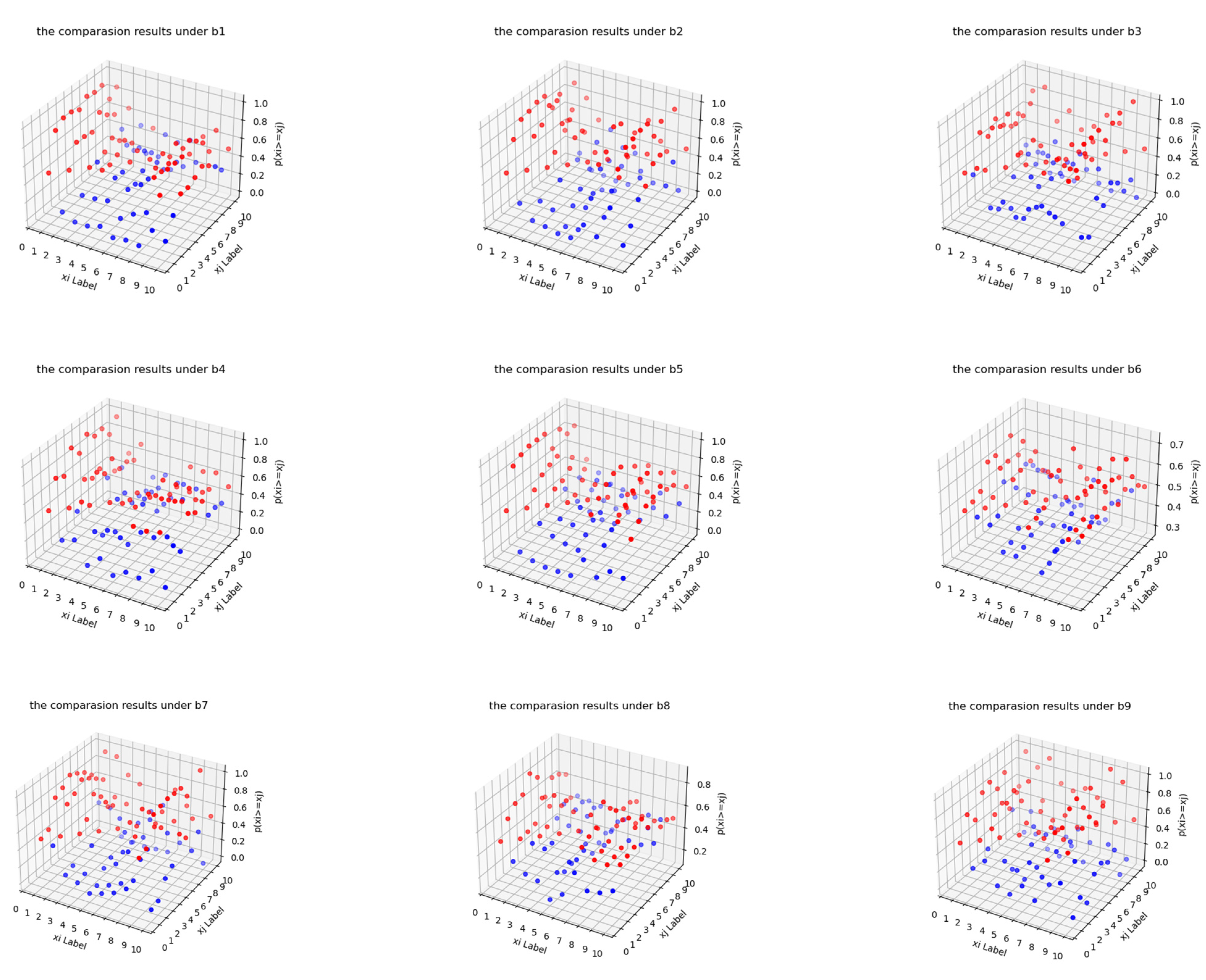
$P^{b_2}$, $P^{b_3}$,..., $P^{b_9}$ can be obtained in the same way; this is omitted due to space limitations. However, in order to display the results more intuitively, we draw the 9 comparison matrix results of $P^{b_k}$ into the following figure (as shown in Figure 5), where the horizontal coordinate 1–10 represents $x_i$ from $x_1$ to $x_{10}$, the vertical coordinate 1–10 represents $x_j$ from $x_1$ to $x_{10}$, and the vertical coordinate represents the probability that the IFNs $x_i$ is greater than $x_j$. In order to better distinguish the relationship between the advantages and disadvantages of objects, we use different colors for display. When $p_{ij}\ge 0.5$, red marks are used; when $p_{ij}<0.5$, blue marks are used.

(2) Take $\alpha =0.5$ and $\beta =0.5$, then the IFPDR can be obtained.

$$\begin{array}{l}{R}_B^{\ge (0.5,0.5)}=\{(x_1,x_1),(x_1,x_2),(x_1,x_3),(x_1,x_4),(x_1,x_5),(x_1,x_6),(x_1,x_7),(x_1,x_8),(x_1,x_9),(x_1,x_{10}),\\ (x_2,x_2),(x_2,x_3),(x_2,x_4),(x_2,x_5),(x_2,x_6),(x_2,x_7),(x_2,x_8),(x_2,x_{10}),(x_3,x_3),(x_3,x_4),\\ (x_3,x_5),(x_3,x_6),(x_3,x_7),(x_3,x_8),(x_3,x_{10}),(x_4,x_4),(x_4,x_5),(x_4,x_6),(x_5,x_5),(x_6,x_5),\\ (x_6,x_6),(x_7,x_4),(x_7,x_5),(x_7,x_6),(x_7,x_7),(x_7,x_8),(x_7,x_{10}),(x_8,x_4),(x_8,x_5),(x_8,x_6),\\ (x_8,x_8),(x_8,x_{10}),(x_9,x_2),(x_9,x_3),(x_9,x_4),(x_9,x_5),(x_9,x_6),(x_9,x_7),(x_9,x_8),(x_9,x_9),\\ (x_9,x_{10}),(x_{10},x_4),(x_{10},x_6),(x_{10},x_6),(x_{10},x_{10})\}\end{array}$$

The corresponding intuitionistic fuzzy probability dominance intercept matrix is as follows:

$$M_B^{\ge (0.5,0.5)}=\left[\begin{array}{cccccccccc}1& 1& 1& 1& 1& 1& 1& 1& 1& 1\\ 0& 1& 1& 1& 1& 1& 1& 1& 0& 1\\ 0& 0& 1& 1& 1& 1& 1& 1& 0& 1\\ 0& 0& 0& 1& 1& 1& 0& 0& 0& 0\\ 0& 0& 0& 0& 1& 0& 0& 0& 0& 0\\ 0& 0& 0& 0& 1& 1& 0& 0& 0& 0\\ 0& 0& 0& 1& 1& 1& 1& 1& 0& 1\\ 0& 0& 0& 1& 1& 1& 0& 1& 0& 1\\ 0& 1& 1& 1& 1& 1& 1& 1& 1& 1\\ 0& 0& 0& 1& 1& 1& 0& 0& 0& 1\end{array}\right]$$

For example: because of $(x_1,x_2)\in R_B^{\ge (0.5,0.5)}$, so $M_B^{\ge (0.5,0.5)}(1,2)=1$, and $(x_2,x_1)\notin R_B^{\ge (0.5,0.5)}$, so $M_B^{\ge (0.5,0.5)}(2,1)=0$ (The first number in parentheses represents the row of the elements in the matrix $M_B^{\ge (0.5,0.5)}$, and the second number represents the column of the elements in the matrix).

(3) The intuitionistic fuzzy probability dominance matrix $C$ can be obtained from the calculation formula in step 3 as follows:

$$C_B^{\ge (0.5,0.5)}=\left[\begin{array}{cccccccccc}1& 3& 4& 8& 10& 9& 5& 6& 2& 7\\ 0& 1& 2& 6& 8& 7& 3& 4& 0& 5\\ 0& 0& 1& 5& 7& 6& 2& 3& 0& 4\\ 0& 0& 0& 1& 3& 2& 0& 0& 0& 0\\ 0& 0& 0& 0& 1& 0& 0& 0& 0& 0\\ 0& 0& 0& 0& 2& 1& 0& 0& 0& 0\\ 0& 0& 0& 4& 6& 5& 1& 2& 0& 3\\ 0& 0& 0& 3& 5& 4& 0& 1& 0& 2\\ 0& 2& 3& 7& 9& 8& 4& 5& 1& 6\\ 0& 0& 0& 2& 4& 3& 0& 0& 0& 1\end{array}\right]$$

For example: denote the second row of $M_B^{\ge (0.5,0.5)}$ as

$$M_B^{\ge (0.5,0.5)}(2,:)=[0,1,1,1,1,1,1,1,0,1]$$

denote the third column of $M_B^{\ge (0.5,0.5)}$ as

$$M_B^{\ge (0.5,0.5)}(:,3)={[1,1,1,0,0,0,0,0,1,0]}^T$$

then $C_B^{\ge (0.5,0.5)}(2,3)$ can be calculated as

$$\begin{array}{l}{C}_B^{\ge (0.5,0.5)}(2,3)=c_{23}=M_B^{\ge (0.5,0.5)}(2,:)\cdot M_B^{\ge (0.5,0.5)}(:,3)\\ =0\times 1+1\times 1+1\times 1+1\times 0+1\times 0+1\times 0+1\times 0+1\times 0+0\times 1+1\times 0\\ =2\end{array}$$

Moreover, we can also compute it in terms of sets, as $c_{23}=|{[x_2]}_B^{\ge (0.5,0.5)}\cap {[x_3]}_B^{\le (0.5,0.5)}|$.

When

$$\begin{gathered} \hspace{1em}\hspace{1em}\hspace{1em}{[x_2]}_B^{\ge (0.5,0.5)}=\{x_2,x_3,x_4,x_5,x_6,x_7,x_8,x_{10}\} \\ {[x_3]}_B^{\le (0.5,0.5)}=\{x_1,x_2,x_3,x_9\} \end{gathered}$$

then ${[x_2]}_B^{\ge (0.5,0.5)}\cap {[x_3]}_B^{\le (0.5,0.5)}=\{x_2,x_3\}$, and $c_{23}=\left|\right\{x_2,x_3\left\}\right|=2$.

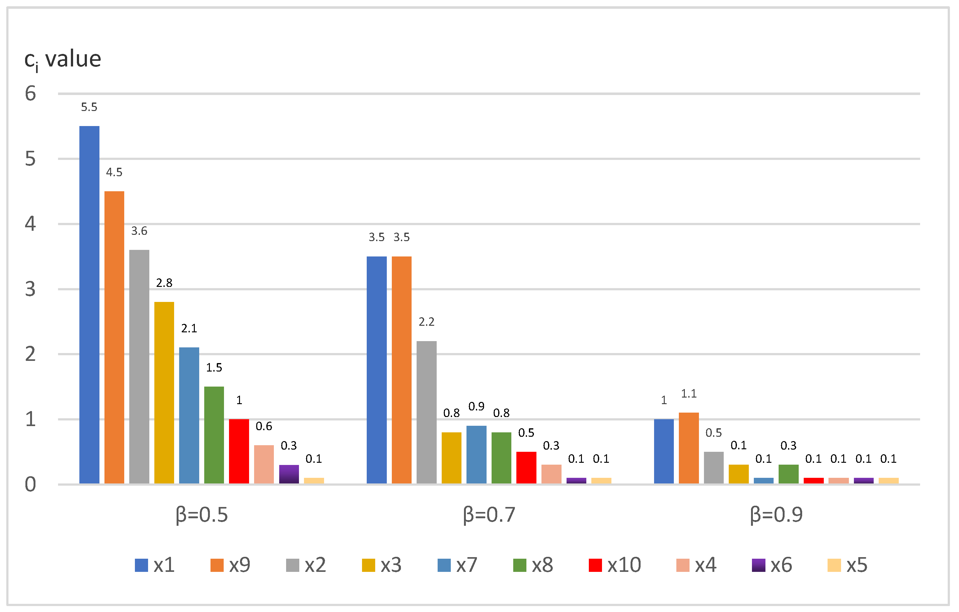
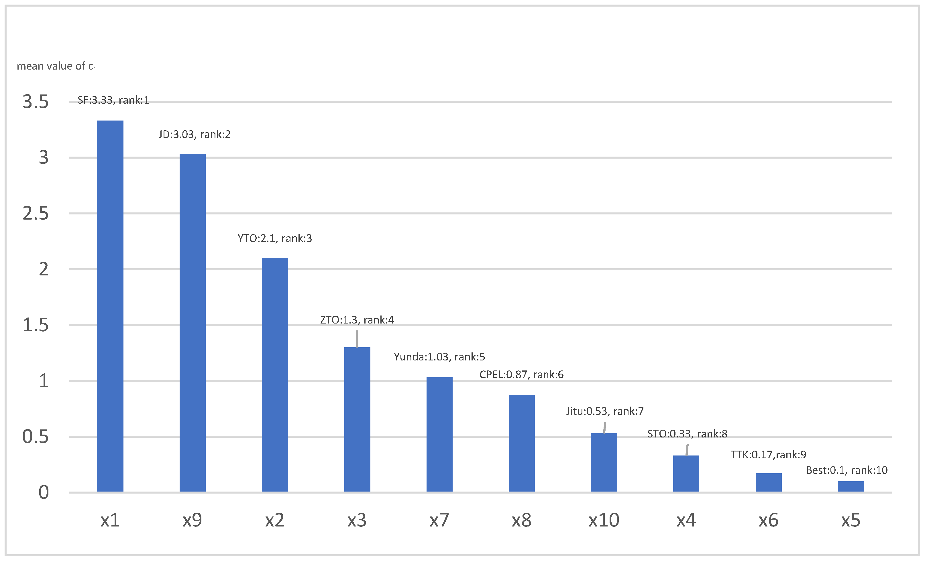
(4) By averaging all lines in $C_B^{\ge (0.5,0.5)}$ by step 4, the comprehensive dominance degree $c_i$ of each object can be obtained. In order to further test the influence of parameter $\beta$, $\beta =0.7,0.9$ is taken for repeated calculation, and the results are shown in Figure 6 and Figure 7.

For example: when $\beta =0.5$, $c_1=(1+3+4+8+10+9+5+6+2+7)/10=5.5$ (as shown in Figure 6), other $c_i$ values can be obtained similarly.

As can be seen from the results of Figure 6, when $\beta =0.5$, it has the strongest differentiation ability and can better distinguish all objects without the situation of parallel ranking. When $\beta =0.7$, $x_1~x_9$, $x_3~x_8$ and $x_5~x_6$ are all the undifferentiated comparison results; when $\beta =0.9$, $x_3~x_8$ and $x_4~x_5~x_6~x_7~x_{10}$ are all the undifferentiated comparison results. It can be seen that the larger $\beta$ is, the weaker the differentiation ability will be, and there will be many cases that cannot be compared. However, the sorting results under different $\beta$ values are not completely consistent, and even reverse order may exist. Therefore, the final result can be the average of the three scenarios. The ranking result is shown in Figure 7, that is, SF Express has the strongest overall strength, followed by JD Express, and Best Express has the worst ranking. This result is basically consistent with the value of the original data and the result of pair-to-pair comparison. Under most indexes, SF Express and JD Express have relatively large DM but relatively small DN while Best Express has relatively small DM and relatively large DN. In the pairwise comparison of objects, there are only five times of probability comparison value less than 0.5 in 90 comparisons of nine indexes of $x_1$ (SF Express), and only six times of probability comparison value less than 0.5 in 81 comparisons of $x_9$ (JD Express) with the exception of comparing to $x_1$. In contrast, $x_5$ (Best Express) only had eight times of probability comparison value greater than 0.5. Therefore, we believe that this ranking result is in line with the actual situation and reasonable.

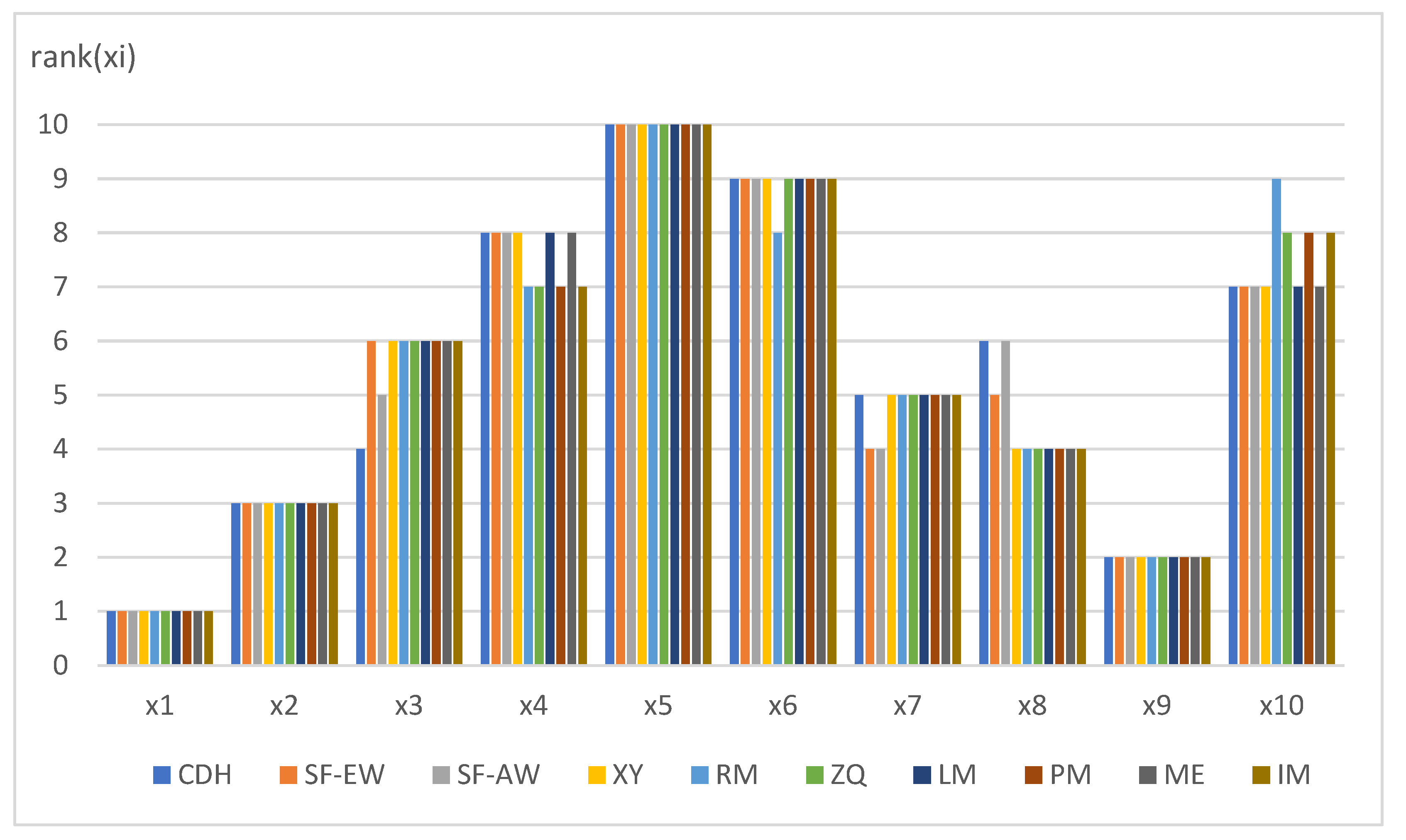
In order to further verify the rationality and effectiveness of the proposed algorithm, various algorithms mentioned in literature [28,53] are selected for comparative analysis, and the final ranking results are shown in Figure 8.

Note: The comparison algorithm in Figure 6 is explained as follows:

Method ① (CDH): The conversion of the DH model proposed in this paper, and the results are as shown in Figure 8.

Method ② (SF-EW): the score function with the entropy weight method, from the literature [28]. Firstly, the score function is calculated for the direct fuzzy number under each attribute. Then, based on the score function, the entropy weight method is used to calculate the weight. Finally, the scheme ranking results are obtained by calculating the comprehensive score function.

Method ③ (SF-AW): the score function with the average weight method, which was obtained from the literature [28]. The value of each attribute is aggregated via the average weight, and other parts are the same as the SF-EW.

Method ④~⑩ (XY, RM, ZQ, LM, PM, ME, and IM): They are all from the literature [53]; the comparison formula of intuitionistic fuzzy numbers refers to the original text. The attribute aggregation methods all adopt the addition principle of multiple intuitionistic fuzzy numbers. In the ZQ method, parameter k = 1.

From Figure 6, we can see that the ranking results of elements under most of the ranking methods are consistent, which also validates the effectiveness of various methods (for example, the ranking results of $x_1$, $x_2$, $x_5$ and $x_9$ under the 10 methods are unchanged, and the ranking results of $x_4$, $x_6$, $x_7$ and $x_{10}$ under different methods differ by 1 bit). It is worth noting that the ranking results of $x_3$ and $x_8$ in this paper differ by 2 bits from those of other comparison methods, and there is a reverse order between them. In other literature, the ranking result is $x_3<x_8$, while the ranking result in this paper is $x_3>x_8$, and we think the ranking result in this paper is more reasonable. As can be seen from the original data, according to the comparison results of this paper, all of the five attributes of $b_2,b_4,b_5,b_6,b_7$ meet $P^{b_i}(x_3\ge x_8)\ge 0.5$, and the proportion of their dominance attributes is 5/9, exceeding the threshold of 0.5. Therefore, it is reasonable to determine the final result as $x_3>x_8$.

6. Discussion

This paper mainly focuses on two aspects. First, aiming at the problem that the IFNs are difficult to compare, we convert the DH into the DM and DN and use the probability method to realize the comparison of IFNs. This method draws on the comparison rules of interval numbers to some extent, but it has strong applicability and can be compared against any IFNs. Secondly, for the MADM problem, we constructed the MADM method based on the probability dominance relation in the form of IFNs. This method does not need to give the weight of different attributes subjectively, the decision result is driven by the original data, and the threshold α and β can be adjusted according to the decision preference of the decision-maker. The proposed method can be well applied to real decision-making problems, and it has wide application prospects.

About the comparison of IFNs, the current research methods mainly propose various measurement formulas for a single IFN, such as score function, precision function and other indicators, and then calculate its indicator value for each IFN, so as to compare between different IFNs. Among these measurement indicators, the measurement formulas in many studies do not consider the influence of DH on the ranking of IFNs, or deal with DH in the same way as DM and DN, and do not fully consider the information uncertainty expressed by DH itself. Relevant scholars often lack an explanation of actual meaning in the measurement formulas they propose. Therefore, the comparison of IFNs in this paper does not measure a single IFN, but is based on the comparison of a pair of IFNs. In the form of paired comparison, the comparison result is not “either–or” ($x>y$ or $x<y$), the comparison result of two IFNs is presented in the form of probability. This method provides a more widely applicable expression for the comparison of IFNs, so that decision makers can choose results under different decision thresholds rather than the only comparison results.

For the MADM problem, the current research mainly aggregates the values under different attributes by constructing various weight operators, but the weight determination is also a difficult problem in the decision-making process. Some scholars use the subjective method to determine the weight, only to verify the feasibility of the method from the perspective of examples, but rarely discuss the sensitivity of the influence of different weights on the decision results. In addition, some scholars adopt the objective weighting method. Common methods mainly include the optimization weight method and entropy weight method, but the optimization method is difficult to calculate the weight. In contrast, the MADM method constructed based on the probability dominance relationship in this paper calculates the proportion of attribute sets satisfying the comparison of advantages and disadvantages by setting thresholds, effectively avoiding the direct aggregation of attributes, and eliminating the need to manually determine attribute weights, thus making the decision results more objective. Compared with the classical dominance relation, the probabilistic dominance relation in this paper appropriately loosens the conditional restrictions, allowing decision-makers to reflect their personal preferences by adjusting the threshold within a certain range. Under extreme conditions, it can also degenerate into the classical dominance relation, which makes the decision results more widely applicable and avoids the decision failure situation, which is easy to exist in the classical dominance relation.

Regarding the two aspects of the research in this paper, further discussion and expansion can be carried out as follows: regarding the comparison of IFNs, this paper did not consider the distribution form of DH as a random variable when converting DH into DM and DN. In the actual analysis of this paper, we derived it according to the simplest uniform distribution form. In fact, if further research is carried out, we can assume the distribution form of random variables in the conversion of DH to be normal distribution, exponential distribution, T-distribution and other forms for more systematic exploration and research. In addition, when constructing the judgment matrix of pairwise comparison, we set the restriction condition of parameter α > 0.5, which requires at least half of the probability of dominance. For this purpose, we can also consider lowering the threshold α further, such as α > 0.3, because the conversion of DH itself has a large uncertainty, so we can assume that as long as $x$ has a 30% probability of superiority over $y$, $x$ still has a high probability of defeating $y$ in the final “duel”. Alternatively, when the decision maker is particularly strict, they may set the threshold α as α > 0.8, which means that a very high probability of dominance is needed to ensure that $x$ is superior to $y$. However, at this time, we will face a problem, that is, the intercept matrix induced by the dominant probability judgment matrix does not satisfy the symmetric complementarity, which makes part of the mathematical properties of the intercept matrix no longer maintained, but it still can give a decision result.

On the other hand, in the MADM model, we construct the decision method based on the probabilistic dominance relation. Here, we still need to determine another threshold β, that is, the lower limit of the proportion of the dominant object when two objects are compared. In this model, we take β > 0.5 as the basic principle. In the case application of Section 5, we discuss β = 0.5, β = 0.7, and β = 0.9, respectively. Similar to the threshold α, we can also consider lowering β below 0.5, which helps each object gain more dominance class elements, but when β is too small (e.g., β = 0.1), this condition becomes almost meaningless. In addition, regarding the setting of threshold α and β, we should follow a “When one is rising, the other is falling” principle, that is, when α is set high, β can be appropriately reduced; in contrast, if α is set low, β can be appropriately increased. If α and β are very low, they will make the dominance class of elements not have advantages, and the comparison is meaningless. Similarly, if α and β are both high, the judgment conditions will be too strict, and the dominance class construction is easy to fail in practical decision problems. Therefore, we give a reference criterion, that is, α + β ≥ 1.

The research method proposed in this paper can be widely used in other fields. As long as multiple attributes are involved and the value of attributes is uncertain, the IFNs-based information system can be constructed for MADM evaluation to some extent. For example, in the evaluation of investment schemes, firstly, the diversification of evaluation indicators makes it impossible to make decisions based on only one indicator, so it conforms to the characteristics of MADM. Secondly, any investment is risky, and its returns are not fixed. According to the different states of the market, we can convert the belonging, unbelonging, and uncertain parts of the indicators value into DM, DN, and DH, respectively, so as to construct the intuitionistic fuzzy information system for decision-making. For another example, in the emotion analysis of natural language processing (using an intelligent customer service chatbot), due to the diversity of language expression meanings, often a word can express both a positive emotion on one occasion and a negative emotion on another occasion. Therefore, the relationship between emotional words and emotional states can also be expressed via IFN, and then, the emotional state of the whole sentence can be expressed by aggregating multiple emotional words. Of course, it can still be expressed as an IFN. The proposed scheme can also be used for path following schemes of intelligent vehicles and multi-robots. In paths following control, road conditions faced by vehicles or robots are often complex, which is difficult to be directly expressed by accurate variables and data. In this case, IFNs provides a feasible scheme. In terms of the control of state variables such as path curvature, vehicle speed, turning angle, and obstacle safety distance, we designed multiple levels for them, expressed their actual values by membership function, which can be converted to DM, DN and DH, and then planned reasonable driving paths for them according to vehicle safety requirements to ensure the flexible response ability and high safety of the path following scheme. There are many other similar occasions, such as supplier selection and evaluation, construction safety and risk assessment, and so on. As long as we can express the data table in the form of IFNs, we can apply the model and method proposed in this paper to solve the corresponding problems.

There are some limitations of this work: firstly, there is limited discussion regarding the properties of IFNs comparison and ranking methods. Secondly, the constructors of the dominance relation and dominance class in the MADM method do not satisfy the monotonicity of the attribute sets (that is, the larger the attribute sets, the smaller the dominance relation and dominance class). Finally, in the case analysis and application section, we did not test a larger data set. These are things that we can try to do better in future studies.

7. Conclusions

The comparison of intuitionistic fuzzy numbers (IFNs) will have an important impact on the theory and method of multi-attribute decision-making (MADM), but the current research has not solved this problem well. Therefore, based on the conversion concept of degree of hesitation (DH), this paper proposes the probabilistic conversion comparison method of IFNs based on the area method, and then constructs the probability dominance relationship model based on IFNs, designs the corresponding MADM method, and finally verifies and applies the model and method through the evaluation problem of campus express stations. The results show that it is scientific and reasonable. However, the research of this paper still has some shortcomings, such as group decision-making problem and multi-granularity decision-making problem based on IFNs; designing better comparison and ranking methods is required in the future.

References

- Zadeh, L.A. Fuzzy sets. Inf. Control 1965, 8, 338–353. [Google Scholar] [CrossRef]
- Wang, C.; Qiang, X.; Xu, M.H.; Wu, T. Recent Advances in Surrogate Modeling Methods for Uncertainty Quantification and Propagation. Symmetry 2022, 14, 1219. [Google Scholar] [CrossRef]
- Luo, M.X.; Li, W.L. Some new similarity measures on picture fuzzy sets and their applications. Soft Comput. 2023, 27, 6049–6067. [Google Scholar] [CrossRef]
- Atanassov, K.T. Intuitionistic Fuzzy Sets. Fuzzy Sets Syst. 1986, 20, 87–96. [Google Scholar] [CrossRef]
- Dan, S.; Kar, M.B.; Majumder, S.; Roy, B.; Pamucar, D. Intuitionistic Type-2 Fuzzy Set and Its Properties. Symmetry 2019, 11, 808. [Google Scholar] [CrossRef]
- Torra, V. Hesitant Fuzzy Sets. Int. J. Intell. Syst. 2010, 25, 529–539. [Google Scholar] [CrossRef]
- Alcantud JC, R.; Santos-Gacia, G.; Peng, X.D.; Zhan, J. Dual Extended Hesitant Fuzzy Sets. Symmetry 2019, 11, 714. [Google Scholar] [CrossRef]
- Liu, J.; Zhang, W.; Chung, Y.; Tang, Z.; Xie, Y.; Ma, T.; Zhang, J.; Zhang, G.; Niyoyita, J.P. Adaptive Intrusion Detection via GA-GOGMM-based Pattern Learning with Fuzzy Rough Set-based Attribute Selection. Expert Syst. Appl. 2020, 139, 112845. [Google Scholar] [CrossRef]
- Syau, Y.R.; Lin, E.B.; Liau, C.J. Fuzzy Binary Rough Set. Int. J. Uncertain. Fuzziness Knowl.-Based Syst. 2020, 28, 317–329. [Google Scholar] [CrossRef]
- Mathew, B.; John, S.J.; Alcantud, J.C.R. Multi-Granulation Picture Hesitant Fuzzy Rough Sets. Symmetry 2020, 12, 362. [Google Scholar] [CrossRef]
- Ayub, S.; Shabir, M.; Riaz, M.; Mahmood, W.; Bozanic, D.; Marinkovic, D. Linear Diophantine Fuzzy Rough Sets: A New Rough Set Approach with Decision Making. Symmetry 2022, 14, 525. [Google Scholar] [CrossRef]
- Gong, Z.T.; Wang, L.W. Covering-based variable precision rough fuzzy set models. J. Lanzhou Univ. Nat. Sci. 2019, 55, 105–112. [Google Scholar]
- Sun, B.; Ma, W.; Chen, X. Variable precision multigranulation rough fuzzy set approach to multiple attribute group decision-making based on λ-similarity relation. Comput. Ind. Eng. 2019, 127, 326–343. [Google Scholar] [CrossRef]
- Yang, J.; Huang, M.Y.; Chen, J. Neighborhood-based multi-granulation rough fuzzy sets and their uncertainty measure. J. Chongqing Univ. Posts Telecommun. (Nat. Sci. Ed.) 2020, 32, 898–908. [Google Scholar]
- Khalil, A.M.; Cao, D.Q.; Azzam, A.; Smarandache, F.; Alharbi, W.R. Combination of the Single-Valued Neutrosophic Fuzzy Set and the Soft Set with Applications in Decision-Making. Symmetry 2020, 12, 1361. [Google Scholar] [CrossRef]
- Pan, L.P.; Deng, Y.; Cheong, K.H. Quaternion model of Pythagorean fuzzy sets and its distance measure. Expert Syst. Appl. 2023, 213, e119222. [Google Scholar] [CrossRef]
- Kumar, K.; Chen, S.M. Group decision making based on entropy measure of Pythagorean fuzzy sets and Pythagorean fuzzy weighted arithmetic mean aggregation operator of Pythagorean fuzzy numbers. Inf. Sci. 2023, 624, 361–377. [Google Scholar] [CrossRef]
- Dai, Z.M.; Hu, K.; Xie, J.; Ya, G. Ensemble Learning Algorithm Based on Intuitionistic Fuzzy Sets. Comput. Sci. 2021, 48, 270–274, 280. [Google Scholar]
- Liu, L.M.; Gong, Y.L.; Cao, W.Z.; Yang, Y. Emergency logistics plan decision-making method based on linguistic intuitionistic fuzzy sets. Comput. Integr. Manuf. Syst. 2021, 27, 1494–1505. [Google Scholar]
- Li, S.M.; Guan, X.; Sun, G.D. Recognition method based on hesitant fuzzy set for unequal length sequences and its application. J. Commun. 2021, 42, 41–51. [Google Scholar]
- Wang, H.W.; Ran, Y.; Zhang, G.B. Comprehensive Evaluation Method for Quantitative Multi-indexes of Manufacturing Process Based on Hesitant Fuzzy Sets. J. Hunan Univ. (Nat. Sci.) 2021, 48, 59–70. [Google Scholar]
- Li, R.X.; Hu, W.X.; Qi, X.L. The Applications of Utility function and Entropy of Interval Type-2 Fuzzy Set in Risk Decision-Making. Oper. Res. Manag. Sci. 2021, 30, 102–109. [Google Scholar]
- Rani, J.J.; Manivannan, A.; Dhanasekar, S. Interval Valued Intuitionistic Fuzzy Diagonal Optimal Algorithm to Solve Transportation Problems. Int. J. Fuzzy Syst. 2023. [Google Scholar] [CrossRef]
- Yang, Y.J.; Chiclana, F. Consistency of 2D and 3D distances of intuitionistic fuzzy sets. Expert Syst. Appl. 2012, 39, 8665–8670. [Google Scholar] [CrossRef]
- Guo, K.H.; Wang, Z.Q. Interval-valued Intuitionistic Fuzzy Knowledge Measure with Applications Based on Hamming-Hausdorff Distance. J. Softw. 2022, 33, 4251–4267. [Google Scholar]
- Sun, G.; Wang, M.X.; Li, X.P.; Huang, W. Distance measure and intuitionistic fuzzy TOPSIS method based on the centroid coordinate representation. J. Intell. Fuzzy Syst. 2023, 41, 555–571. [Google Scholar] [CrossRef]
- Ullah, K.; Mahmood, T.; Jan, N. Similarity Measures for T-Spherical Fuzzy Sets with Applications in Pattern Recognition. Symmetry 2018, 10, 193. [Google Scholar] [CrossRef]
- Pan, F.P.; Gong, R.C.; Tan, K.X. Multi-attribute group decision-making method for tourism projects based on interval intuitionistic fuzzy information. Stat. Decis. 2021, 37, 173–176. [Google Scholar]
- Deng, X.Y.; Yang, Y.; Jiang, W. Discrete choice models with Atanassov-type intuitionistic fuzzy membership degrees. Inf. Sci. 2023, 622, 46–67. [Google Scholar] [CrossRef]
- Qin, H.W.; Li, H.F.; Ma, X.Q.; Gong, Z.; Cheng, Y.; Fei, Q. Data Analysis Approach for Incomplete Interval-Valued Intuitionistic Fuzzy Soft Sets. Symmetry 2020, 12, 1061. [Google Scholar] [CrossRef]
- Das, A.K.; Granados, C. IFP-intuitionistic multi fuzzy N-soft set and its induced IFP-hesitant N-soft set in decision-making. J. Ambient Intell. Humaniz. Comput. 2022. [Google Scholar] [CrossRef]
- Guo, Z.L.; Yang, H.L.; Wang, J. Intuitionistic fuzzy probabilistic rough set model on two universes and its applications. Syst. Eng. Theory Pract. 2014, 34, 1828–1834. [Google Scholar]
- Huang, X.H.; Zhang, X.Y.; Yang, J.L. Two-Universe Multi-granularity Probability Rough Sets Based on Intuitionistic Fuzzy Relations. Pattern Recognit. Artif. Intell. 2022, 35, 439–450. [Google Scholar]
- Gong, Z.T.; Ta, G.P. Semantics of the soft set induced by intuitionistic fuzzy set and its three-way decision. J. Shandong Univ. (Nat. Sci.) 2022, 57, 68–76. [Google Scholar]
- Liu, J.B.; Peng, L.S.; Li, H.X.; Huang, B.; Zhou, X. Interval-valued Intuitionistic Fuzzy Three Way Group Decisions Considering The Unknown Weight Information. Oper. Res. Manag. Sci. 2022, 31, 50–57. [Google Scholar]
- Li, X.N.; Zhao, L.; Yi, H.J. Three-way decision of intuitionistic fuzzy information systems based on the weighted information entropy. Control Decis. 2022, 37, 2705–2713. [Google Scholar]
- Dai, J.H.; Chen, T.; Zhang, K. The intuitionistic fuzzy concept-oriented three-way decision model. Inf. Sci. 2023, 619, 52–83. [Google Scholar] [CrossRef]
- Chao, N.; Wan, R.X.; Miao, D.Q. Neighborhood Rough Set Based on Dominant Relation in Intuitionistic Fuzzy Information System. J. Shanxi Univ. (Nat. Sci. Ed.) 2023, 46, 62–68. [Google Scholar]
- Xue, Z.A.; Lv, M.J.; Han, D.J.; Xin, X. Multi-Granulation Graded Rough Intuitionistic Fuzzy Sets Models Based on Dominance Relation. Symmetry 2018, 10, 446. [Google Scholar] [CrossRef]
- Li, D.F.; Lin, P. An intuitionistic fuzzy Bayesian network bidirection reasoning model for stampede fault diagnosis analysis of scenic spots integrating the D-S evidence theory. Syst. Eng.-Theory Pract. 2022, 42, 1979–1992. [Google Scholar]
- Peng, Y.; Liu, X.H.; Sun, J.B. Interval-Valued Intuitionistic Fuzzy Multi-attribute Group Decision Making Approach Based on the Hesitancy Degrees and Correlation Coefficient. Chin. J. Manag. Sci. 2021, 29, 229–240. [Google Scholar]
- Batool, N.; Hussain, S.; Kausar, N.; Munir, M.; Li, R.; Khan, S. Decision Making under Incomplete Data: Intuitionistic Multi Fuzzy Ideals of Near-Ring Approach. Decis. Mak. Appl. Manag. Eng. 2023, 5, 67–89. [Google Scholar]
- Kong, R.; Zhao, N. Merchant Ranking based on Intuitionistic Fuzzy Sentiment and Dual-attention BILSTM[J/OL]. J. Syst. Manag. 2022, 1–21. Available online: http://kns.cnki.net/kcms/detail/31.1977.N.20221228.1659.002.html (accessed on 9 January 2023).
- Fu, C.; Zhou, S.S.; Zhang, D.; Chen, L. Relative Density-Based Intuitionistic Fuzzy SVM for Class Imbalance Learning. Entropy 2023, 25, 34. [Google Scholar] [CrossRef] [PubMed]
- Wei, C.P.; Liang, X.; Zhang, Y.Z. A Comparative Analysis and Improvement of Entropy Measure for Intuitionistic Fuzzy Sets. J. Syst. Sci. Math. Sci. 2012, 32, 1437–1448. [Google Scholar]
- Sevastjanov, P.; Dymova, L.; Kaczmarek, K. A new approach to the comparison of real, interval and fuzzy-valued intuitionistic fuzzy and Belief-Plausibility numbers. Int. J. Approx. Reason. 2023, 152, 262–281. [Google Scholar] [CrossRef]
- Wang, Y.; Lei, Y.J.; Lu, Y.L. Multiple attribute decision making method based on intuitionistic fuzzy sets. Syst. Eng. Electron. 2007, 29, 2060–2063. [Google Scholar]
- Zhao, F.X. Distances Between Interval-Valued Intuitionistic Fuzzy Sets. Microelectron. Comput. 2010, 27, 188–192. [Google Scholar]
- Li, Y.H.; Sun, G. A unified ranking method of intuitionistic fuzzy numbers and Pythagorean fuzzy numbers based on geometric area characterization. Comput. Appl. Math. 2023, 42, e16. [Google Scholar] [CrossRef]
- Ye, J. Cosine similarity measure for intuitionistic fuzzy sets and their applications. Math. Comput. Model. 2011, 53, 91–97. [Google Scholar] [CrossRef]
- Xie, J.M.; Liu, S.Y. Similarity Measure of Interval Valued Intuitionistic Fuzzy Sets and Its Application. Math. Pract. Theory 2018, 48, 249–255. [Google Scholar]
- Xu, C.L.; Chen, J.H. New distance between intuitionistic fuzzy sets and its applications in decision-making. Appl. Res. Comput. 2020, 37, 3627–3634. [Google Scholar]
- Liang, M.S.; Mi, J.S.; Zhang, S.P.; Jin, C. A novel approach for ranking intuitionistic fuzzy numbers and its application to decision making. J. Intell. Fuzzy Syst. 2023, 44, 661–672. [Google Scholar] [CrossRef]
Figure 1.
α-probability conversion of the IFN.
Figure 2.
The change trend of conversion DM of and with different conversion probabilities .
Figure 3.
Position relation of IFNs.
Figure 4.
MADM method block diagram.
Figure 5.
Dominance degree matrix under different attributes.
Figure 6.
Comparison of the ranking results at different values.
Figure 7.
The final raking result of express delivery points with mean value of .
Figure 8.
Comparison of ranking results of different algorithms.