
Bounds for Extreme Zeros of Classical Orthogonal Polynomials Related to Birth and Death Processes

1
Department of Mathematics and Statistics, College of Science, King Faisal University, Al Hasa 31982, Saudi Arabia
2
Department of Mathematics, National Institute of Technology Jamshedpur, Jamshedpur 831014, Jharkhand, India
*
Author to whom correspondence should be addressed.
†
These authors contributed equally to this work.
Symmetry 2023, 15(4), 890; https://doi.org/10.3390/sym15040890
Submission received: 2 March 2023
/
Revised: 6 April 2023
/
Accepted: 8 April 2023
/
Published: 10 April 2023
(This article belongs to the Special Issue Symmetries of Difference Equations, Special Functions and Orthogonal Polynomials II)
Abstract
:In this paper, we consider birth and death processes with different sequences of transition rates and find the bound for the extreme zeros of orthogonal polynomials related to the three term recurrence relations and birth and death processes. Furthermore, we find the related chain sequences. Using these chain sequences, we find the transition probabilities for the corresponding process. As a consequence, transition probabilities related to G-fractions and modular forms are derived. Results obtained in this work are new and several graphical representations and numerical computations are provided to validate the results.
1. Introduction
Let us consider the second order differential equation
where and are polynomials independent of n, is known as the eigenvalue parameter which depends on [1,2] and and e are real parameters. In the self-adjoint form of (1), the general weight function is given by
The parameters d and e in (2) depend on three independent parameters a, b and c. Consequently, we will have exactly six solutions of Equation (1) known as classical orthogonal polynomials (COPS). Classical orthogonal polynomials and Sturm–Liouville problems are also related to symmetry (see [3]). Classical orthogonal polynomials can also be characterized as finite COPS and infinite sequences. Jacobi, Leguerre and Hermite orthogonal polynomials are three well-known cases of infinite orthogonal sequences while the other three finite COPS are less familiar in the literature. In [4], Masjed-Jamei characterized the finite cases and studied various properties. For details of this literature we refer to [4,5,6,7] and references cited therein. In [4], these finite COPS are categorized as first, second and third classes, based on their connection with Jacobi, Hermite and Bessel functions, respectively. The R-Jacobi, R-Hermite, and R-Bessel polynomials can also be used to represent these classes of polynomials. Here, R- stands for Routh or Romonovski, because Routh [8] and Romonovski [9] introduced and studied these classes independently. For further details regarding this literature can be found in [5,6,9] and references cited therein. In [5,6], Malik and Swaminathan called these R-Jacobi, R-Hermite and R-Bessel finite COPS as Type I, Type II and Type III COPS, respectively. The following Table 1 gives details of all the six classical orthogonal polynomials.
Let be a sequence of classical orthogonal polynomials. Then it satisfies the following three term recurrence relation
with for . COPS have lot of applications in mathematical biology, queueing theory and other fields of pure and applied mathematics. In this paper, we consider the applications of COPS, especially R-Jacobi and R-Bessel polynomials in birth and death processes. Before proceeding towards the main results, let us provide a short introduction about birth and death processes.
A special case of the continuous time Markov process is the birth and death process whose transition probabilities are defined as
and states are labelled by non-negative integers.
Let and be birth and death rates, respectively, for and . Then the transition probabilities satisfy the following
Theorem 1
([10] Theorem 5.2.1). Transition probabilities satisfy the following Chapman–Kolmogorov differential equations
It is well known that birth and death processes and orthogonal polynomials are related to each other [10,11].
Let
The family of polynomials are called birth and death polynomials.
The following theorem describes the behaviour of zeros of birth and death process polynomials.
Theorem 2
([10] Theorem 7.2.5). The zeros of birth and death process polynomials belong to .
In this paper, our objective is to find the bounds for the extreme zeros of the finite classes of orthogonal polynomials related to birth and death processes with the help of chain sequences.
Definition 1
(Chain Sequences [12]). A sequence is called a chain sequence if there exists a sequence such that
- (i)
- (ii)
- ,
where the sequence is known as the parameter sequence for .
Let us recall the following well-known results, which will be useful to prove the main results of this manuscript.
Lemma 1
Theorem 3
Then the zeros of lie in .
In 1924, G. U. Yule [14] considered the simplest model of birth and death processes. In [15], quartic transition rates of birth and death processes have been studied. Recently, new Nevanlinna matrices for orthogonal polynomials related to cubic birth and death processes have been derived in [16]. In [13], bounds for extreme zeros of Laguerre, associated Laguerre, Meixner, and MeixnerPollaczek polynomials have been found by M. E. H. Ismail and X. Li. These polynomials are also related to birth and death processes. The above results motivate us to consider R-Jacobi and R-Bessel polynomials and relate them with the birth and death processes and derive the bounds for extreme zeros of these polynomials.
2. R-Jacobi Polynomials Related to Birth and Death Processes
R-Jacobi polynomials are defined as follows ([4], Equation (2.2)):
where and .
The polynomials satisfy the following differential Equation ([4], Equation (2.1))
The orthogonality relation for these polynomials is given in the following theorem.
Theorem 4
([4] Corollary 2).
if and only if: and
These polynomials can also be expressed [4] in terms of hypergeometric function [17] as follows:
where denotes hypergeometric function [17], with the notation , defined as
Theorem 5.
Let and be the largest and smallest zeros of R-Jacobi polynomials . Then
where
Proof.
First, we consider the following three term recurrence relation ([4], Equation (2.19)) of R-Jacobi polynomials:
Using (8) and (17), it can be easily shown that R-Jacobi polynomials are related to birth and death processes with transition rates
Using Lemma 1, we obtain the chain sequence related to R-Jacobi polynomials as follows:
Finally, using Theorem 3 with the condition and recurrence relation (17), we obtain the required result. □
3. R-Bessel Polynomials Related to Birth and Death Processes
R-Bessel polynomials are defined as [4]
These polynomials are solutions of the following differential equation
The orthogonality relation for these polynomials is given in the following theorem:
Theorem 6
Theorem 7.
Let and be the largest and smallest zeros of R-Bessel polynomials . Then
where
Proof.
It is well-known that R-Bessel polynomials satisfy the following three term recurrence relation ([4], Equation (4.19)):
With the help of (8) and (21), it can be shown that R-Bessel polynomials are related to birth and death processes with transition rates
The chain sequence related to R-Bessel polynomials is given by
Finally, using Theorem 3 with the condition and recurrence relation (21), the required result can be obtained. □
4. Birth and Death Processes with Different Sequences of Transition Rates
In this section, we will derive bounds for the smallest and largest zeros of birth and death process polynomials.
Theorem 8.
Let and be the largest and smallest zeros of birth and death process polynomials with transition rates and . Then
where
Proof.
Now, we will use Theorem 3 to complete the proof. Putting the above values of and in (12) with , the required result can be established. □
5. Birth and Death Processes Related to g-Fraction
In this section, we consider a special type of birth and death process with rates satisfying the condition
with . Clearly, is a chain sequence.
Applying Laplace transform of as
in (5) and (6) with initial state we have
which results in the following S-fraction
This implies
which is the g-fraction. The relationship (29) can be expressed in terms of ratio of hypergeometric functions [18] (pp. 337–339) as follows
Again applying [19] (Theorem 2.1) in (29), we can conclude that the Laplace transform of transition probabilities can be expressed as the ratio of basic hypergeometric functions as follows
for and be such that and .
The polynomials in (32) can be expressed as follows
We are interested to analyse (30). For this we need to compute the roots of . It can be observed that the is zero when is an eigenvalue of the following tridiagonal matrix
The eigenvalues of the above matrix are real and distinct [20] as the above matrix can be transformed into a tridiagonal matrix which is real, symmetric and positive definite whose subdiagonal elements are nonzero. Therefore (27) converges in the s-plane cut from 0 to ∞ along the negative real axis. Let be the roots of . Then (30) can be expressed as [21]
Applying an inverse Laplace transform to the above expression results in
Using the formula (35) we will find the transition probabilities for the following models.
5.1. Model(a)
In this model, we established the chain sequence related to R-Jacobi polynomials.
Clearly, and for . Furthermore, it can be noted that and
which is the chain sequence related to R-Jacobi polynomials.
5.2. Model(b)
It can be easily seen that and for . Furthermore, and
which is the chain sequence related to R-Bessel polynomials.
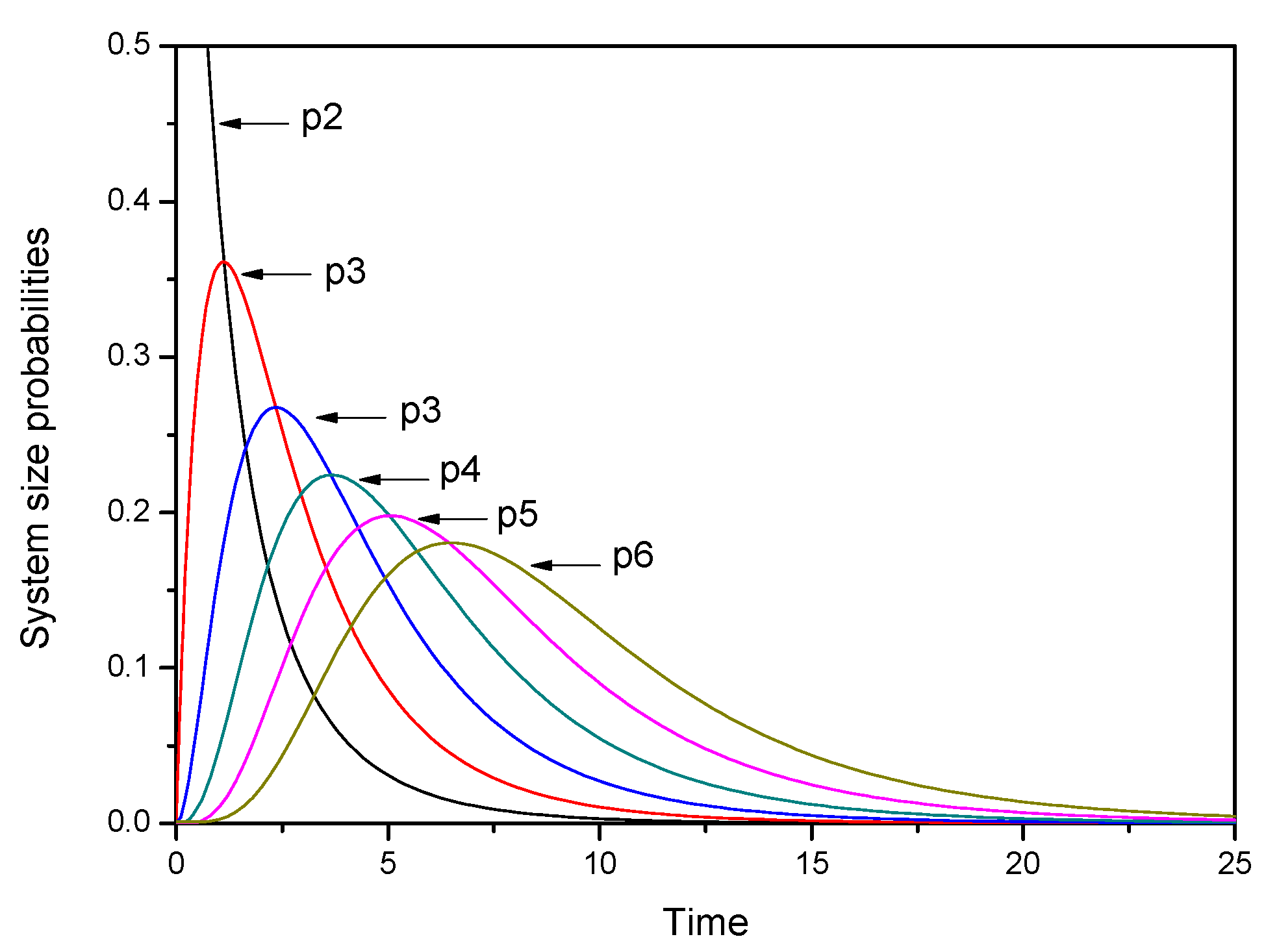
Transition probabilities for this model are computed with numerical values in Table 7.
Time-dependent system size probabilities for model(b) are plotted in Figure 2.
5.3. Model(c)
It can be noted that and for . Further and
which is the chain sequence related to Laguerre polynomials [13].
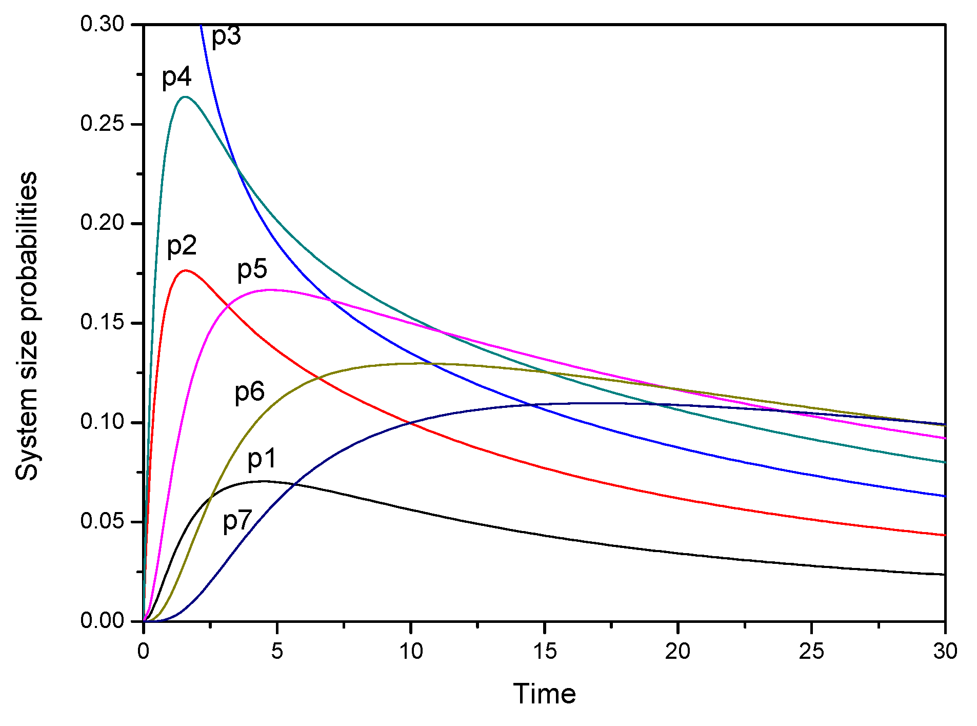
Transition probabilities for this model are computed with numerical values in Table 8.
Time-dependent system size probabilities for model(c) are plotted in Figure 3.
6. Birth and Death Processes Related to Modular Forms
In this section, we consider a special type of birth and death process with transition rates satisfying
where and .
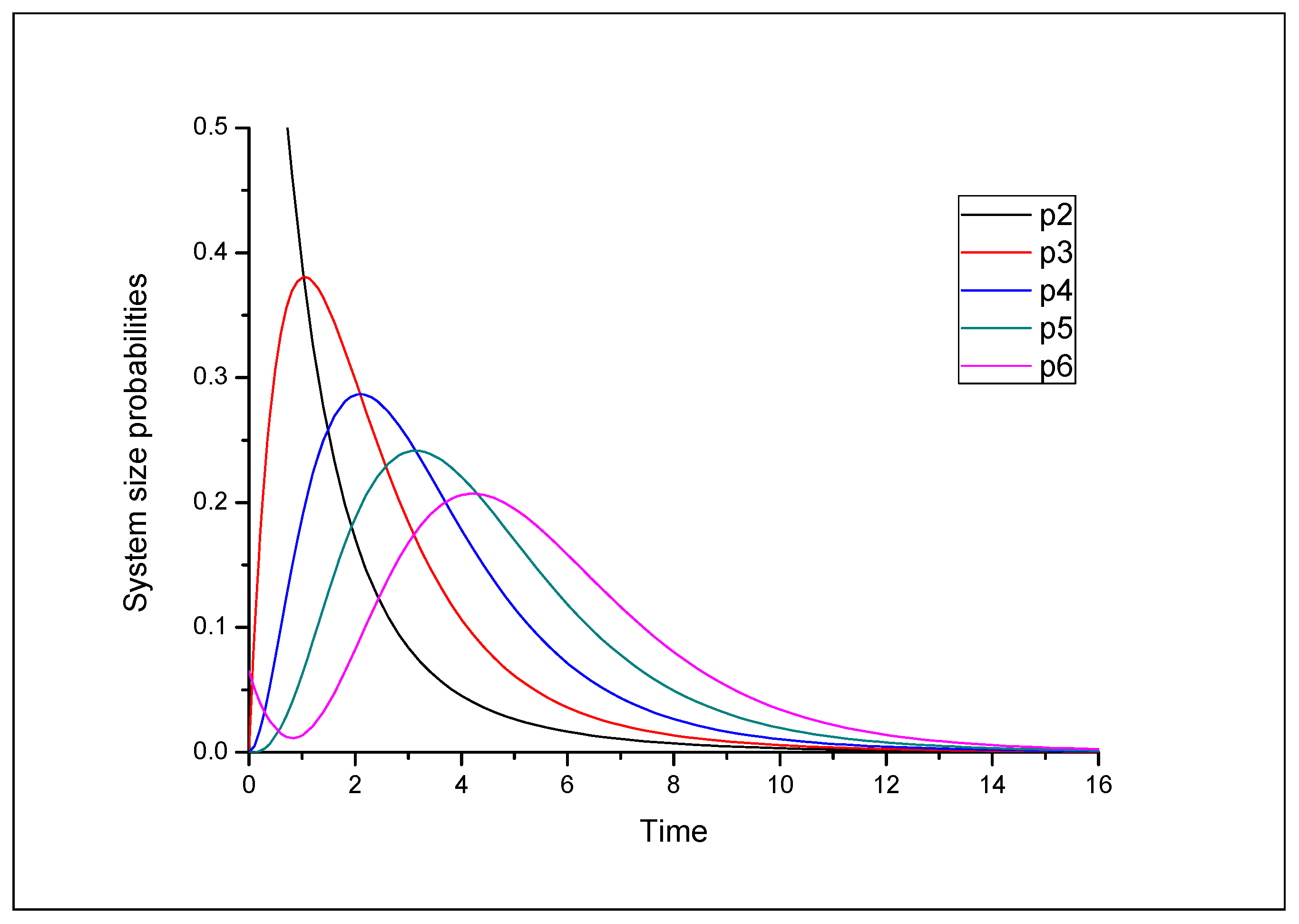
Transition probabilities for this model are computed with numerical values in Table 9.
Time-dependent system size probabilities for this model are plotted in Figure 4.
7. Conclusions
This article finds bounds for the zeros of classical polynomials that are related to birth and death processes. As an application, transition probabilities related to g-fractions and modular forms are derived. The results are validated through numerical examples. Three different models have been considered and numerical values of transition probabilities have been computed for those models.
Author Contributions
Conceptualization, S.R.M. and S.D.; methodology, S.R.M. and S.D.; software, S.D.; validation, S.R.M. and S.D.; formal analysis, S.R.M. and S.D.; investigation, S.R.M. and S.D.; resources, S.R.M. and S.D.; writing—original draft preparation, S.D.; writing—review and editing, S.R.M. and S.D.; visualization, S.R.M. and S.D. All authors have read and agreed to the published version of the manuscript.
Funding
This work was supported by the Deanship of Scientific Research, Vice Presidency for Graduate Studies and Scientific Research, King Faisal University, Saudi Arabia [Grant No. 2268].
Data Availability Statement
Not applicable.
Conflicts of Interest
The authors declare no conflict of interest.
References
- Al-Salam, W.A. Characterization theorems for orthogonal polynomials. In Orthogonal Polynomials (Columbus, OH, 1989); Kluwer Academic Publishers: Dordrecht, The Netherlands, 1990; Volume 294, pp. 1–24. [Google Scholar]
- Nikiforov, A.F.; Uvarov, V.B.; Suslov, S.K. Classical orthogonal polynomials of a discrete variable. In Classical Orthogonal Polynomials of a Discrete Variable; Springer: Berlin/Heidelberg, Germany, 1991; pp. 18–54. [Google Scholar]
- Masjed-Jamei, M. A generalization of classical symmetric orthogonal functions using a symmetric generalization of Sturm-Liouville problems. Integral Transform. Spec. Funct. 2007, 18, 871–883. [Google Scholar] [CrossRef] [Green Version]
- Masjed-Jamei, M. Three finite classes of hypergeometric orthogonal polynomials and their application in functions approximation. Integral Transform. Spec. Funct. 2002, 13, 169–190. [Google Scholar] [CrossRef]
- Malik, P.; Swaminathan, A. Derivatives of a finite class of orthogonal polynomials defined on the positive real line related to F-distribution. Comput. Math. Appl. 2011, 61, 1180–1189. [Google Scholar] [CrossRef] [Green Version]
- Malik, P.; Swaminathan, A. Derivatives of a finite class of orthogonal polynomials related to inverse gamma distribution. Appl. Math. Comput. 2012, 218, 6251–6262. [Google Scholar] [CrossRef]
- Das, S.; Swaminathan, A. Higher order derivatives of R-Jacobi polynomials. AIP Conf. Proc. 2016, 1739, 020058. [Google Scholar]
- Routh, E.J. On some properties of certain solutions of a differential equation of the second order. Proc. Lond. Math. Soc. 1884, 1, 245–262. [Google Scholar] [CrossRef] [Green Version]
- Romanovski, V. Sur quelques classes nouvelles de polynomes orthogonaux. CR Acad. Sci. Paris 1929, 188, 1023–1025. [Google Scholar]
- Ismail, M.E.H. Classical and Quantum Orthogonal Polynomials in One Variable; Encyclopedia of Mathematics and Its Applications; Van Assche, W., Askey, R.A., Eds.; Cambridge University Press: Cambridge, UK, 2005; Volume 98, p. xviii+706. [Google Scholar] [CrossRef]
- Ismail, M.E.H.; Masson, D.R.; Letessier, J.; Valent, G. Birth and death processes and orthogonal polynomials. In Orthogonal Polynomials (Columbus, OH, 1989); Kluwer Academic Publishers: Dordrecht, The Netherlands, 1990; Volume 294, pp. 229–255. [Google Scholar] [CrossRef]
- Chihara, T.S. An Introduction to Orthogonal Polynomials; Mathematics and Its Applications; Gordon and Breach Science Publishers: New York, NY, USA; London, UK; Paris, France, 1978; Volume 13, p. xii+249. [Google Scholar]
- Ismail, M.E.H.; Li, X. Bound on the extreme zeros of orthogonal polynomials. Proc. Amer. Math. Soc. 1992, 115, 131–140. [Google Scholar] [CrossRef]
- Yule, G.U. A Mathematical Theory of Evolution, Based on the Conclusions of Dr. J. C. Willis, F.R.S. Philos. Trans. R. Soc. Lond. 1925, B213, 21–87. [Google Scholar]
- Valent, G. Asymptotic analysis of some associated orthogonal polynomials connected with elliptic functions. SIAM J. Math. Anal. 1994, 25, 749–775. [Google Scholar] [CrossRef]
- Gilewicz, J.; Leopold, E.; Valent, G. New Nevanlinna matrices for orthogonal polynomials related to cubic birth and death processes. J. Comput. Appl. Math. 2005, 178, 235–245. [Google Scholar] [CrossRef] [Green Version]
- Rainville, E.D. Special Functions; The Macmillan Company: New York, NY, USA, 1960; p. xii+365. [Google Scholar] [CrossRef]
- Wall, H.S. Analytic Theory of Continued Fractions; D. Van Nostrand Co., Inc.: New York, NY, USA, 1948; p. xiii+433. [Google Scholar]
- Baricz, A.; Swaminathan, A. Mapping properties of basic hypergeometric functions. J. Class. Anal. 2014, 5, 115–128. [Google Scholar] [CrossRef] [Green Version]
- Wilkinson, J.H. The Algebraic Eigenvalue Problem; Monographs on Numerical Analysis; Oxford University Press: New York, NY, USA, 1988; p. xviii+662. [Google Scholar]
- Parthasarathy, P.R.; Lenin, R.B.; Schoutens, W.; Van Assche, W. A birth and death process related to the Rogers–Ramanujan continued fraction. J. Math. Anal. Appl. 1998, 224, 297–315. [Google Scholar] [CrossRef] [Green Version]
- Murphy, J.A.; O’Donohoe, M.R. Some properties of continued fractions with applications in Markov processes. J. Inst. Math. Appl. 1975, 16, 57–71. [Google Scholar] [CrossRef]
- Folsom, A. Modular forms and Eisenstein’s continued fractions. J. Number Theory 2006, 117, 279–291. [Google Scholar] [CrossRef] [Green Version]
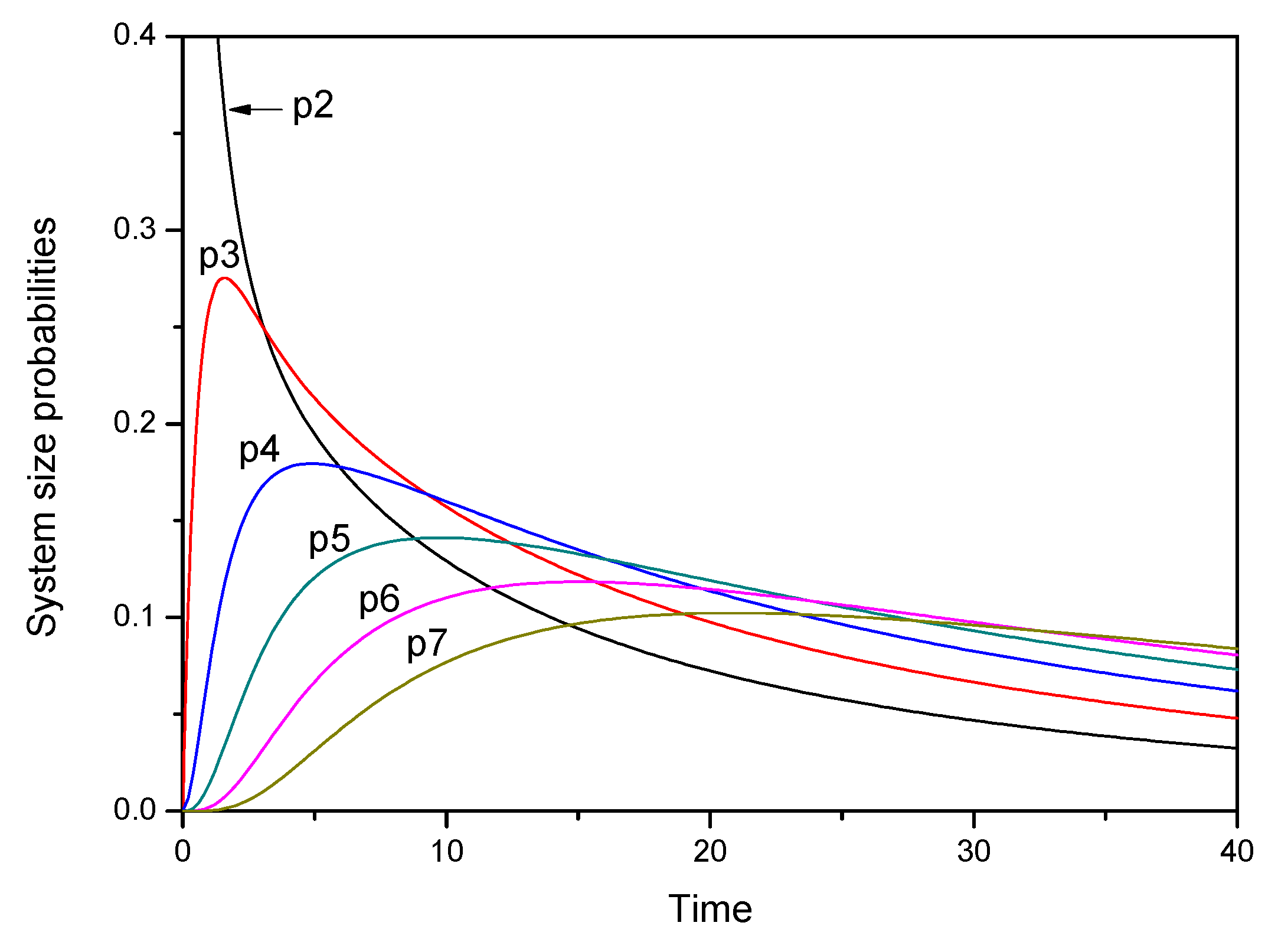
Figure 1.
Time-dependent system size probabilities pr in time t for model(a) with , , , and .

Figure 2.
Time-dependent system size probabilities pr in time t for model(b) with , , and

Figure 3.
Time-dependent system size probabilities pr in time t for model(c) with , , and .

Figure 4.
Time-dependent system size probabilities pr in time t with , and .


Table 1.
Characteristics of classical orthogonal polynomials.
| Type | Polynomial | Weight Function | Interval | ||
|---|---|---|---|---|---|
| Jacobi | |||||
| Infinite | Laguerre | x | |||
| Hermite | 1 | ||||
| R-Jacobi | |||||
| Finite | R-Hermite | ||||
| R-Bessel |
Table 2.
Upper and lower bounds for different values of p, q and n.
| Value of p, q, n | A | S(n, p, q) | L(n, p, q) | B |
|---|---|---|---|---|
| p = 30, q = 1, n = 5 | 0.000848214 | 0.025003868 | 0.182868373 | 0.677473464 |
| p = 100, q = 3, n = 5 | 0.003256378 | 0.015689532 | 0.052264761 | 0.306032160 |
| p = 50, q = 5, n = 10 | 0.013386412 | 0.036491151 | 0.399137716 | 2.334827874 |
| p = 150, q = 10, n = 20 | 0.0075034407 | 0.015606200 | 0.235232011 | 1.100631480 |
Table 3.
Upper and lower bounds for different values of p and n.
| Values of p, n | A | S(n,p) | L(n,p) | B |
|---|---|---|---|---|
| p = 60, n = 25 | 0.0174143242 | 0.001100195 | 0.127635714 | 1.232585676 |
| p = 50, n = 20 | 0.0175690519 | 0.001590043 | 0.108368111 | 1.024097615 |
| p = 70, n = 30 | 0.0177484733 | 0.000807141 | 0.146851849 | 1.440584860 |
| p = 90, n = 40 | 0.0192205990 | 0.000489853 | 0.185209710 | 1.855779401 |
Table 4.
Upper and lower bounds for cubic rates for .
| Value of n | B | A |
|---|---|---|
| n = 1 | 99.47726751 | 0.52273249 |
| n = 2 | 672.2966054 | −2.2966054 |
| n = 3 | 2326.965295 | −6.965295 |
| n = 4 | 5709.384764 | −11.384764 |
| n = 5 | 11467.58306 | −15.583056 |
Table 5.
Upper and lower bounds for quartic rates for .
| Value of n | B | A |
|---|---|---|
| n = 1 | 1294.470417 | 1.5295830 |
| n = 2 | 14248.78880 | −16.788798 |
| n = 3 | 69140.94425 | −116.94425 |
Table 6.
Transition probabilities for model(a), with , , .
| m | r | |||||||
|---|---|---|---|---|---|---|---|---|
| 1 | 2 | 0.2921490112 | 0.2361484997 | 0.1522190975 | 0.1072492705 | 0.08052549270 | 0.06306134397 | 0.05080189081 |
| 3 | 0.08716742291 | 0.2132663566 | 0.1738894810 | 0.1346557113 | 0.1065579573 | 0.08641940405 | 0.07149194738 | |
| 5 | 0.00238032673 | 0.08378329415 | 0.1339337865 | 0.1354764126 | 0.1240258026 | 0.1104448910 | 0.09768734107 | |
| 7 | 0.00002430702 | 0.01601707595 | 0.06178924538 | 0.08982065195 | 0.1002648982 | 0.1012550939 | 0.09777580080 | |
| 2 | 2 | 0.4687113670 | 0.1946394431 | 0.1291172295 | 0.09425915593 | 0.07241108386 | 0.05755657124 | 0.04682820943 |
| 3 | 0.2603710210 | 0.2132973859 | 0.1571127893 | 0.1219534631 | 0.09755450156 | 0.07987002622 | 0.06655452399 | |
| 4 | 0.07401956616 | 0.1794384547 | 0.1598844328 | 0.1349421989 | 0.1136304110 | 0.09641486357 | 0.08256032205 | |
| 5 | 0.01387332775 | 0.1205803453 | 0.1411610078 | 0.1327425518 | 0.1190445276 | 0.1053936555 | 0.09312573082 | |
| 3 | 3 | 0.4666402935 | 0.1885109146 | 0.1333550248 | 0.1050671356 | 0.08556482599 | 0.07106591813 | 0.05985421345 |
| 4 | 0.2468602213 | 0.1974994012 | 0.1489883379 | 0.1221831980 | 0.1027761281 | 0.08763755703 | 0.07546816996 | |
| 5 | 0.06813638099 | 0.1623296273 | 0.1451025641 | 0.1270522000 | 0.1115151393 | 0.09815261276 | 0.08668459066 | |
| 6 | 0.01252210876 | 0.1074754172 | 0.1250247001 | 0.1202487741 | 0.1114387753 | 0.1018850330 | 0.09263129043 | |
| 5 | 2 | 0.0000964846760 | 0.0004029736173 | 0.0001109421737 | 0.00002487661389 | 0.000006292446081 | 0.000001903841593 | 6.850542824 (−7) |
| 5 | 0.4209957064 | 0.06081681946 | 0.01238287855 | 0.003239382078 | 0.001017418311 | 0.0003745677399 | 0.0001569887786 | |
| 6 | 0.3398204028 | 0.1224310542 | 0.02808273894 | 0.007687593257 | 0.002460489906 | 0.0009101597456 | 0.0003817757263 | |
| 8 | 0.0415780272 | 0.2028401500 | 0.08635305934 | 0.02965021464 | 0.01063284278 | 0.004185138909 | 0.001821109112 |
Table 7.
Transition probabilities for model(b), with , .
| m | r | |||||||
|---|---|---|---|---|---|---|---|---|
| 2 | 0.3668649512 | 0.07064456326 | 0.006122786352 | 0.0007672220517 | 0.0001418440957 | 0.00003666418262 | 0.00001214606363 | |
| 1 | 3 | 0.1701546382 | 0.1407243071 | 0.01888675760 | 0.002811271418 | 0.0005568489677 | 0.0001468292158 | 0.00004891825431 |
| 4 | 0.0514906594 | 0.1941662333 | 0.04309915220 | 0.007886154548 | 0.001711514829 | 0.0004670552694 | 0.0001572694753 | |
| 5 | 0.011469638 | 0.2027097044 | 0.07762512167 | 0.01796275083 | 0.004359471899 | 0.001249481701 | 0.0004285528284 | |
| 2 | 0.3996490201 | 0.03099278684 | 0.003026111462 | 0.0004488996456 | 0.00009492395743 | 0.00002695810522 | 0.000009473396079 | |
| 2 | 3 | 0.3593382733 | 0.08604679375 | 0.01055212421 | 0.001724092631 | 0.0003786025130 | 0.0001084563680 | 0.00003828579884 |
| 4 | 0.1613757455 | 0.1540740571 | 0.02712850599 | 0.005095887598 | 0.001188222539 | 0.0003474884220 | 0.0001234936488 | |
| 8 | 0.003519920 | 0.1095910381 | 0.1503713552 | 0.06828797038 | 0.02481924585 | 0.009082332113 | 0.003603371537 | |
| 2 | 0.002239066965 | 0.002137757004 | 0.0003764044042 | 0.00007070476114 | 0.00001648642933 | 0.000004821355533 | 0.000001713457916 | |
| 4 | 3 | 0.04864064014 | 0.01377958392 | 0.002193064577 | 0.0004416671154 | 0.0001122602281 | 0.00003534534684 | 0.00001326656829 |
| 4 | 0.4151999358 | 0.05131643936 | 0.008681826526 | 0.001953416698 | 0.0005483642480 | 0.0001866026873 | 0.00007398207589 | |
| 7 | 0.04213035014 | 0.2022873297 | 0.07641991533 | 0.02328205397 | 0.007537792533 | 0.002735338567 | 0.001118752499 | |
| 2 | 0.0000032881816 | 0.00006422126647 | 0.00002925499766 | 0.000008079660527 | 0.000002258345658 | 7.149512291 (−7) | 2.617673046 (−7) | |
| 6 | 5 | 0.06542941236 | 0.02357301641 | 0.005407082951 | 0.001480178073 | 0.0004737455651 | 0.0001752432074 | 0.00007350753874 |
| 6 | 0.4257098799 | 0.06962097613 | 0.01643030578 | 0.004860655269 | 0.001677931965 | 0.0006615582574 | 0.0002913915376 | |
| 8 | 0.1374600047 | 0.1855299209 | 0.06208661130 | 0.02088652821 | 0.007708531309 | 0.003156124400 | 0.001425209067 |
Table 8.
Transition probabilities for model(c), with , .
| m | r | |||||||
|---|---|---|---|---|---|---|---|---|
| 2 | 0.4688267232 | 0.1928633801 | 0.1264207062 | 0.09218781872 | 0.07136666125 | 0.05757133172 | 0.04781824363 | |
| 2 | 3 | 0.2653438205 | 0.2168648054 | 0.1584100418 | 0.1226725479 | 0.09856504753 | 0.08152856675 | 0.06897910514 |
| 5 | 0.01443626936 | 0.1256558025 | 0.1467547469 | 0.1377028448 | 0.1236393294 | 0.1100037303 | 0.09802573107 | |
| 6 | 0.00201432251 | 0.06987523393 | 0.1153935846 | 0.1237887813 | 0.1197378807 | 0.1117862083 | 0.1030428725 | |
| 1 | 0.02917435854 | 0.07005180573 | 0.05612717942 | 0.04319081505 | 0.03424686358 | 0.02800919288 | 0.02349067590 | |
| 3 | 2 | 0.1667875442 | 0.1363150204 | 0.09957202627 | 0.07710845857 | 0.06195517271 | 0.05124652764 | 0.04335829463 |
| 3 | 0.4672718500 | 0.1903502007 | 0.1348745875 | 0.1065555416 | 0.08744076768 | 0.07355224355 | 0.06302933573 | |
| 6 | 0.01281660035 | 0.1106226948 | 0.1296802361 | 0.1253706875 | 0.1167654692 | 0.1074488453 | 0.09853498511 | |
| 1 | 0.004006093074 | 0.03490131784 | 0.03804604903 | 0.03301105450 | 0.02790196141 | 0.02374149645 | 0.02045846387 | |
| 4 | 3 | 0.1753337072 | 0.1753337072 | 0.1072362467 | 0.08824142863 | 0.07467112357 | 0.06429071854 | 0.05610744881 |
| 5 | 0.2409534358 | 0.1926145016 | 0.1456727717 | 0.1223972416 | 0.1067395368 | 0.09465581698 | 0.08478676156 | |
| 6 | 0.06540061567 | 0.1559532589 | 0.1395179853 | 0.1239369090 | 0.1116997349 | 0.1014857762 | 0.09267627585 | |
| 5 | 1 | 0.000429767008 | 0.01498158082 | 0.02362958641 | 0.02372314186 | 0.02167960266 | 0.01936335494 | 0.01724682791 |
| 3 | 0.03659875165 | 0.08779175077 | 0.07903155670 | 0.06950029549 | 0.06132142863 | 0.05439130069 | 0.04854685473 | |
| 5 | 0.4663702967 | 0.1861249691 | 0.1320798136 | 0.1091642271 | 0.09506946368 | 0.08469292916 | 0.07634551417 | |
| 6 | 0.2351733252 | 0.1871505923 | 0.1405394533 | 0.1181891252 | 0.1041888019 | 0.09388609320 | 0.08557504052 |
Table 9.
Transition probabilities with , .
| m | r | |||||||
|---|---|---|---|---|---|---|---|---|
| 2 | 2 | 0.3900357047 | 0.02658584041 | 0.003251737369 | 0.0004999903630 | 0.00007840736855 | 0.00001231747087 | 0.000001935350659 |
| 3 | 0.3756794991 | 0.06058285595 | 0.005664561651 | 0.0008170697324 | 0.0001272010066 | 0.00001996780969 | 0.000003137153307 | |
| 4 | 0.1859163290 | 0.1139863351 | 0.01033550057 | 0.001335267686 | 0.0002037521180 | 0.00003190719536 | 0.000005011638279 | |
| 6 | 0.03459111 | 0.1941578052 | 0.03413503594 | 0.003762703845 | 0.0005154609431 | 0.00007893180696 | 0.00001235816122 | |
| 3 | 1 | 0.0004630194876 | 0.0004580759529 | 0.00008060843377 | 0.00001278455567 | 0.000002010595418 | 3.159439443 (−7) | 4.964323829 (−8) |
| 2 | 0.01014334649 | 0.001635737113 | 0.0001529431649 | 0.00002206088278 | 0.000003434427186 | 5.391308622 (−7) | 8.470313934 (−8) | |
| 4 | 0.3701921713 | 0.03976083628 | 0.001070262814 | 0.00006825537042 | 0.000009072098519 | 0.000001398890914 | 2.193776390 (−7) | |
| 5 | 0.1845293945 | 0.09157906054 | 0.003444466194 | 0.0001486194938 | 0.00001516582457 | 0.000002237431245 | 3.491270317 (−7) | |
| 4 | 2 | 0.00004065990305 | 0.00002492881147 | 0.000002260373975 | 2.920230428 (−7) | 4.456058821 (−8) | 6.978103621 (−9) | 1.096045292 (−9) |
| 3 | 0.002998556596 | 0.0003220627739 | 0.000008669128788 | 5.528685000 (−7) | 7.348399796 (−8) | 1.133101637 (−8) | 1.776958875 (−9) | |
| 4 | 0.3698214230 | 0.007688259764 | 0.00007926891020 | 0.000001612886673 | 1.268093942 (−7) | 1.823425381 (−8) | 2.840614969 (−9) | |
| 6 | 0.1841254981 | 0.08628876235 | 0.002513625449 | 0.00004505149497 | 9.149910149 (−7) | 5.327583632 (−8) | 7.116594456 (−9) |
Disclaimer/Publisher’s Note: The statements, opinions and data contained in all publications are solely those of the individual author(s) and contributor(s) and not of MDPI and/or the editor(s). MDPI and/or the editor(s) disclaim responsibility for any injury to people or property resulting from any ideas, methods, instructions or products referred to in the content. |
© 2023 by the authors. Licensee MDPI, Basel, Switzerland. This article is an open access article distributed under the terms and conditions of the Creative Commons Attribution (CC BY) license (https://creativecommons.org/licenses/by/4.0/).
Share and Cite
MDPI and ACS Style
Mondal, S.R.; Das, S. Bounds for Extreme Zeros of Classical Orthogonal Polynomials Related to Birth and Death Processes. Symmetry 2023, 15, 890. https://doi.org/10.3390/sym15040890
AMA Style
Mondal SR, Das S. Bounds for Extreme Zeros of Classical Orthogonal Polynomials Related to Birth and Death Processes. Symmetry. 2023; 15(4):890. https://doi.org/10.3390/sym15040890
Chicago/Turabian StyleMondal, Saiful R., and Sourav Das. 2023. "Bounds for Extreme Zeros of Classical Orthogonal Polynomials Related to Birth and Death Processes" Symmetry 15, no. 4: 890. https://doi.org/10.3390/sym15040890
Note that from the first issue of 2016, this journal uses article numbers instead of page numbers. See further details here.