

A Novel Safe Life Extension Method for Aircraft Main Landing Gear Based on Statistical Inference of Test Life Data and Outfield Life Data

1
School of Aeronautic Science and Engineering, Beihang University, Beijing 100191, China
2
Beijing Aeronautical Technology Research Center, Beijing 100076, China
*
Author to whom correspondence should be addressed.
Symmetry 2023, 15(4), 880; https://doi.org/10.3390/sym15040880
Submission received: 10 March 2023
/
Revised: 31 March 2023
/
Accepted: 4 April 2023
/
Published: 7 April 2023
(This article belongs to the Special Issue Advances and Applications of Uncertainty Theory in Reliability and Systems Engineering)
Abstract
:Safe life extension work is demanded on an aircraft’s main landing gear (MLG) when the outfield MLG reaches the predetermined safe life. Traditional methods generally require costly and time-consuming fatigue tests, whereas they ignore the outfield data containing abundant life information. Thus, this paper proposes a novel life extension method based on statistical inference of test and outfield life data. In this method, the MLG’s fatigue life is assumed to follow a right-skewed lognormal distribution with an asymmetric probability density function. In addition, the MLG’s new safe life can be inferred through the Bayesian approach in which the test life data and outfield life data are used for prior information acquisition and Bayesian update, respectively. The results indicated that the MLG’s safe life was significantly extended, illustrating the effectiveness of the proposed method. Numerous simulations also demonstrated that the extended safe life can meet the requirements of reliability and confidence and thus is applicable in engineering practice.
1. Introduction
Flight hours, flight cycles, and calendar time are three life indicators for aircraft, and flight-cycle life is mainly determined by the landing gear (LG) [1]. The LG is one of an aircraft’s main load-bearing structures and the most critical component in the aircraft’s take-offs, landings, and ground activities [2]. During service, the LG are repeatedly subjected to loads caused by landing impact, ground roll, wheel braking, aircraft turning, and other sources, making structural fatigue the primary failure mode [3,4]. Especially for the main landing gear (MLG), it may bear hundreds of tons of aircraft weight or landing shock during service. Once fatigue fracture occurs in critical parts, it will cause serious consequences such as crash accidents. According to surveys, about 60% of aircraft failures are related to the LG, and fatigue is the primary failure type [5]. In addition, in the maintenance accident statistics of transport aircraft from 2003 to 2017, the LG failure is also listed as one of the most common aircraft failures [6]. Therefore, it is essential to ensure the LG’s safety and reliability during its service life.
Due to the characteristics of the single force transmission path, no redundant structure, and heavy load, the MLG is generally constructed with high-strength materials such as high-strength steel and titanium alloy. The fatigue critical crack length of the material is small, and the crack propagation time is short [7,8]. Thus, most countries adopt the safe life design concept for the MLG’s service life determination [9,10]. Since metal structures present obvious individual differences in the fatigue crack initiation time and the time data do not satisfy the symmetry assumption of a normal distribution, the MLG’s fatigue life is generally assumed to follow the lognormal or Weibull distribution [11,12,13,14]. During the MLG’s safe life, it should be ensured with high confidence and reliability (i.e., survival rate) that no fatigue crack occurs [11]. In engineering practice, conducting full-scale fatigue life tests is the most direct and effective way to determine the safe life of aircraft components, including MLG [15,16,17]. The MLG’s safe life is obtained by dividing the test life by the fatigue scatter factor [12], where the scatter factor is related to the life distribution form, reliability requirement, confidence requirement, and the test sample amount [1,18]. For example, in the GJB 67.6A-2008 “military airplane structural strength specification” from China, a full-scale fatigue test with at least four times its service life is required before delivery for the MLG’s verification [19].
In statistics, the MLG’s safe life takes the one-sided lower confidence limit of its reliable life with the required confidence of and required reliability of [20]. In other words, the safe life is an estimate of the reliable life. It is related to the test sample and demanded to be less than the actual value of reliable life with the probability of . During the MLG’s safe life determination, the life test amount is small (generally only one), and the test sample may not even fail. Thus, the estimated safe life is generally far lower than the actual value of the reliable life, resulting in a significant waste of service life potential [21]. When numerous MLGs reach this safe life, safe life extension work has to be performed to improve economic efficiency.
Nowadays, the MLG’s safe life extension in engineering practice is still commonly realized by conducting a full-scale fatigue test on one outfield MLG [17], leading to a costly and time-consuming process [21,22,23]. For example, a full-scale fatigue test of 44,000 flight cycles over eight years was conducted to verify the safe life (11,000 flight cycles) of the Y-8 aircraft [24]. In fact, hundreds of sorties are in service for many types of aircraft, and large amounts of MLG life data will be accumulated during their service. These data also contain much statistical information on reliability assessment. Especially with the rise of individual tracking technologies such as load monitoring, for the landing gear, the outfield life data can be conveniently recorded and converted with the equivalent damage principle [15,25,26]. Since the outfield life data are generated in actual service, they are even more authentic than the test data in the lab before delivery. However, these outfield life data have neither been developed in the MLG’s safe life determination nor safe life extension.
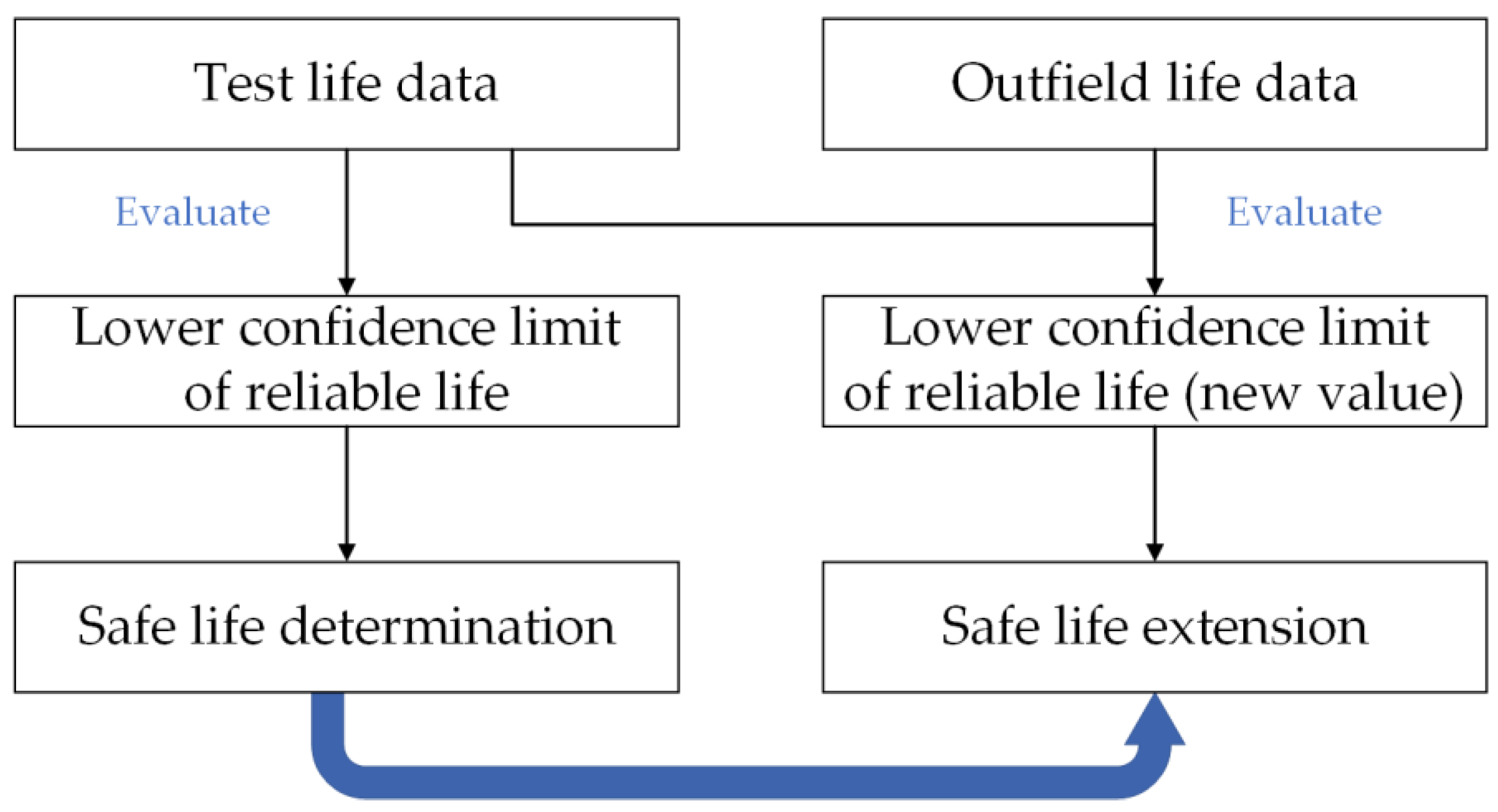
Therefore, as shown in Figure 1, if the MLG’s life data before delivery and in outfield service can be comprehensively developed, a new lower confidence limit of the MLG’s reliable life can be statistically inferred, and the new estimated safe life will be closer to the actual value of reliable life than the safe life determined before delivery because of the added information. In this case, the MLG’s safe life extension can be realized without additional full-scale life tests. Therefore, this paper aimed to achieve the MLG’s safe life extension based on the statistical inference of these life data.
This paper is organized as follows. Section 2 illustrates the MLG’s safe life extension method in detail. On this basis, Section 3 provides a safe life extension example, and Section 4 conducts the simulations for the method’s verifications. Finally, Section 5 presents a summary of the research in this paper.
2. Safe Life Extension Method for MLG
2.1. MLG’s Safe Life Determination by Test Life Data
In general, the MLG’s full-scale fatigue life test consumes a great deal of test time and costs. Thus, only one full-scale life test can be conducted before delivery to determine the MLG’s safe life.
Assume that the MLG’s life follows a lognormal distribution, a commonly used asymmetric life distribution [27,28], and the test life is . Then, the lower confidence limit of the MLG’s reliable life with the confidence and reliability can be determined by [1,18]
and
In the equations, is the fatigue scatter factor, is the standard deviation of the logarithmic life , , and , where is the cumulative distribution function of the standard normal distribution. The lower confidence limit of the reliable life is also called the MLG’s safe life, and it satisfies
where is the actual value of the MLG’s reliable life with the reliability , and it satisfies
In the safe life determination, the value of reliability and confidence are designated by the industrial department. The standard deviation parameter is a known value [1,18]. When the scatter factor is given (generally 4.0–6.0 [12,29]), can be solved by
Table 1 lists the values of and in common use. Among them, the reliability is required to be 0.999, and the confidence is required to be 0.90 or 0.95.
This section introduces the MLG’s safe life determination method currently applied in engineering practice. During the MLG’s outfield service, strict life management is performed with the determined safe life to ensure safety and reliability. On this basis, the MLG’s safe life extension method is further proposed.
2.2. MLG’s Safe Life Extension by Outfield Life Data
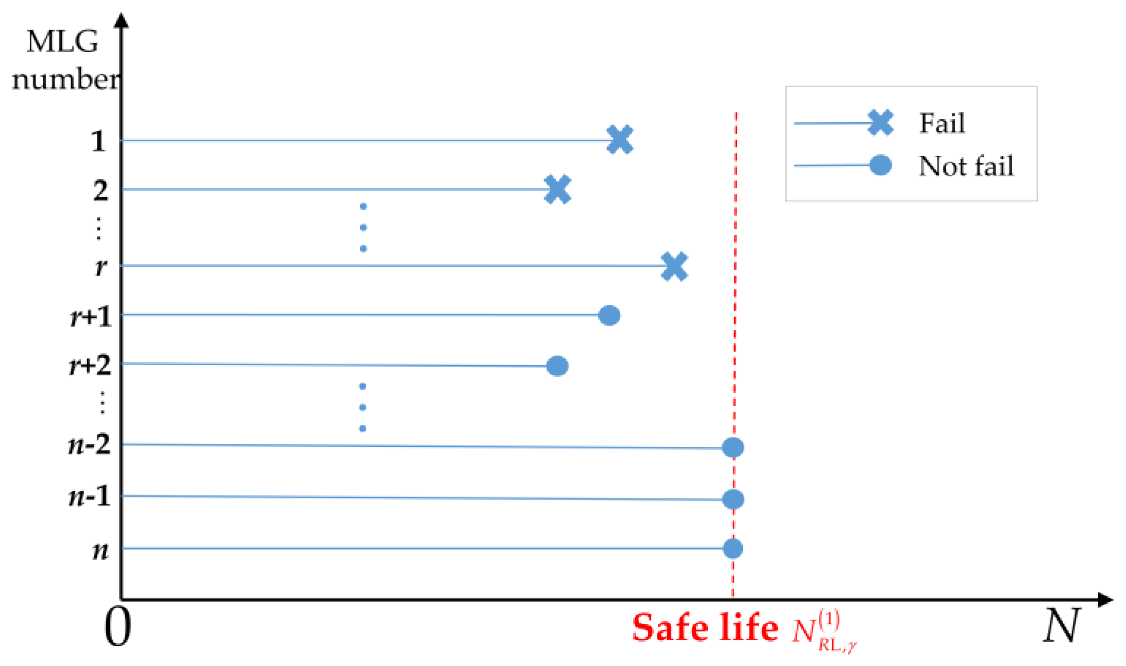
Assume that there are MLGs in the outfield service, and all or part of the MLGs have reached the determined safe life in Equation (1) as shown in Figure 2. Denote the accumulated outfield service life data as , . For general consideration, the first data are assumed to be failure data, and the last data are assumed to be non-failure data.
These outfield service data are generated in the aircraft’s actual flights, making these data even more authentic than the MLG’s test data in the factory. Similar to the test data, the outfield data also contain valuable statistical information about the MLG’s safe life. If such numerous outfield life data can be developed and utilized, the information amount for safe life evaluation can be expanded. Then, a new value of the MLG’s safe life can be obtained. Because more information is used for statistical inference, the new value of the MLG’s safe life will be closer to the MLG’s reliable life while ensuring the reliability and confidence requirements.
However, the MLG’s life data from the fatigue test and outfield service are right-censored, making the statistical inference challenging. Although several algorithms such as maximum likelihood and Bootstrap have been developed to estimate confidence limits of reliability characteristics with censored life data, the estimates are generally approximate [27]. Bayesian is effective for small-sample cases but is limited by the selection of prior distribution [30,31]. This paper adopted the fiducial distribution inferred from the test life data as the prior distribution. Thus, the objectivity of Bayesian inference was ensured. Based on that, the MLG’s safe life extension process is given below.
Firstly, according to the MLG’s test result , the lower confidence limit of the MLG’s logarithmic reliable life with the confidence and reliability can be calculated as [1,18]
It satisfies
where is the actual value of the MLG’s logarithmic reliable life with the reliability . It is worth noting that the MLG’s life after being logarithmic follows a symmetric normal distribution, thus simplifying the discussion. This is one of the advantages of the lognormal distribution.
Then, the confidence of can be updated to through the MLG’s outfield data . The value of can be calculated using the following equations:
where can be 104, 105, 106, or other values according to the numerical precision requirement, and should be an integer. The confidence updating process is realized by the Bayesian approach; the specific formula derivation can be found in Appendix A. It is worth noting that the prior distribution is obtained by the test data , and the likelihood function is constructed by the outfield data . Since the prior distribution is directly obtained by the actual test data instead of subjective assumption, the calculated posterior probability in the Bayesian approach is objective and accurate.
By using Equations (8)–(12), the confidence of is updated from to . Denote . This means that the new confidence of is .
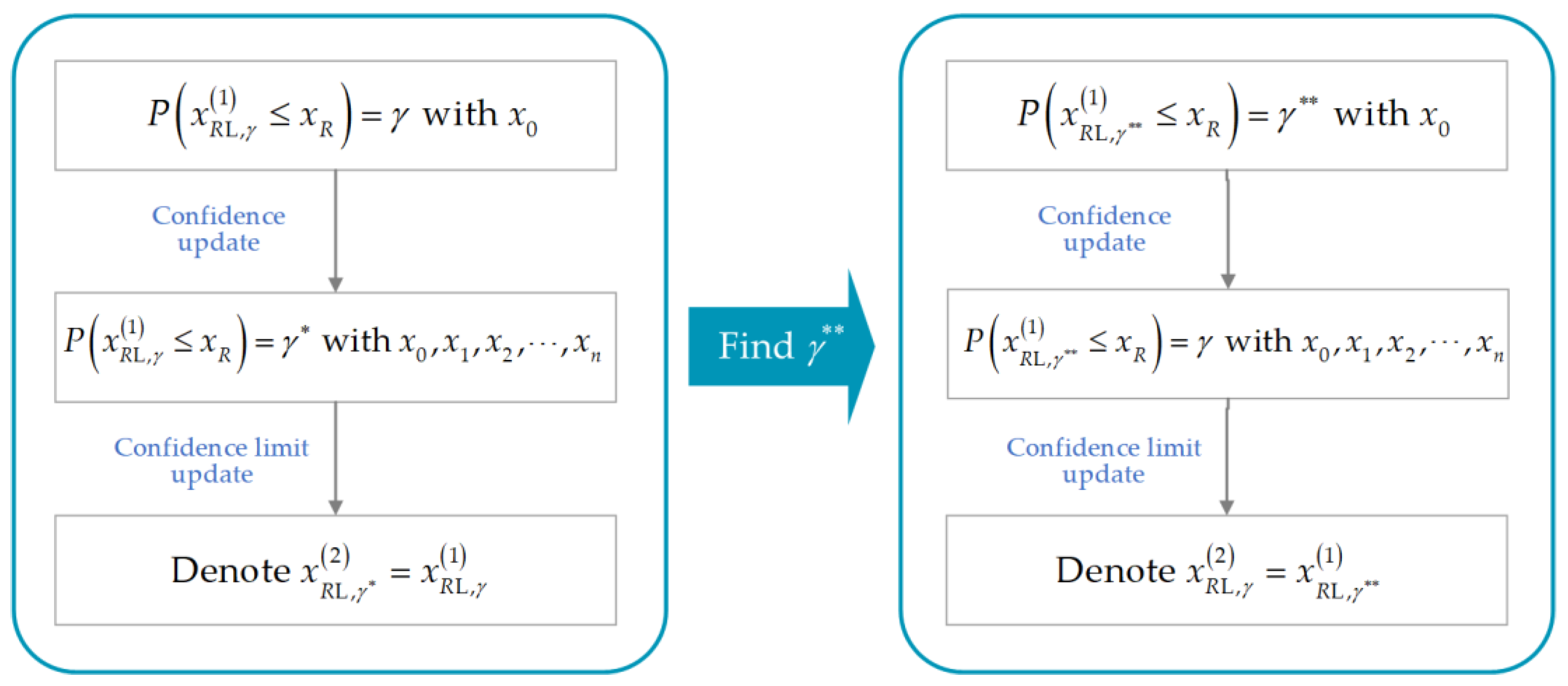
Afterward, adjust the value of in Equation (12) to until the calculated in Equation (8) is equal to the required value of . In other words, find the value of such that . In this case, the lower confidence limit of the MLG’s logarithmic reliable life with the required confidence and reliability can be updated from to , where
For a clear description, Figure 3 illustrates the above lower confidence limit updating process for the MLG’s logarithmic reliable life.
Finally, the MLG’s safe life with the required confidence and reliability is extended form to , where
This satisfies
So, the MLG’s safe life extension under lognormal distribution has been realized.
It can be found that the MLG’s safe life extension is achieved through the mining of the outfield life data and the increasing of the safe life evaluation information. Since this method only performs statistical analysis of the outfield life data without additional MLG full-scale life testing, the cost of safe life extension can be reduced. Meanwhile, the outfield life data are obtained from actual service, which is more authentic and credible than the test life data obtained by simulated loading in the factory. Thus, the extended safe life is convincing.
Remarkably, two extreme cases need to be additionally noted.
When the outfield data are zero-failure data (r = 0), Equation (9) should be simplified as
When the outfield service data are all failure data (r = n), Equation (9) should be simplified as
Then, the analytical solutions of and can be transformed to the classical confidence limit formula form calculated by the complete life data , ; that is [1,18]:
and
The proof for this particular case can be found in Appendix B. Although the situation impossibly appears in engineering practice, it proves the correctness of the MLG’s safe life extension method to a certain extent.
3. Safe Life Extension Example for MLG
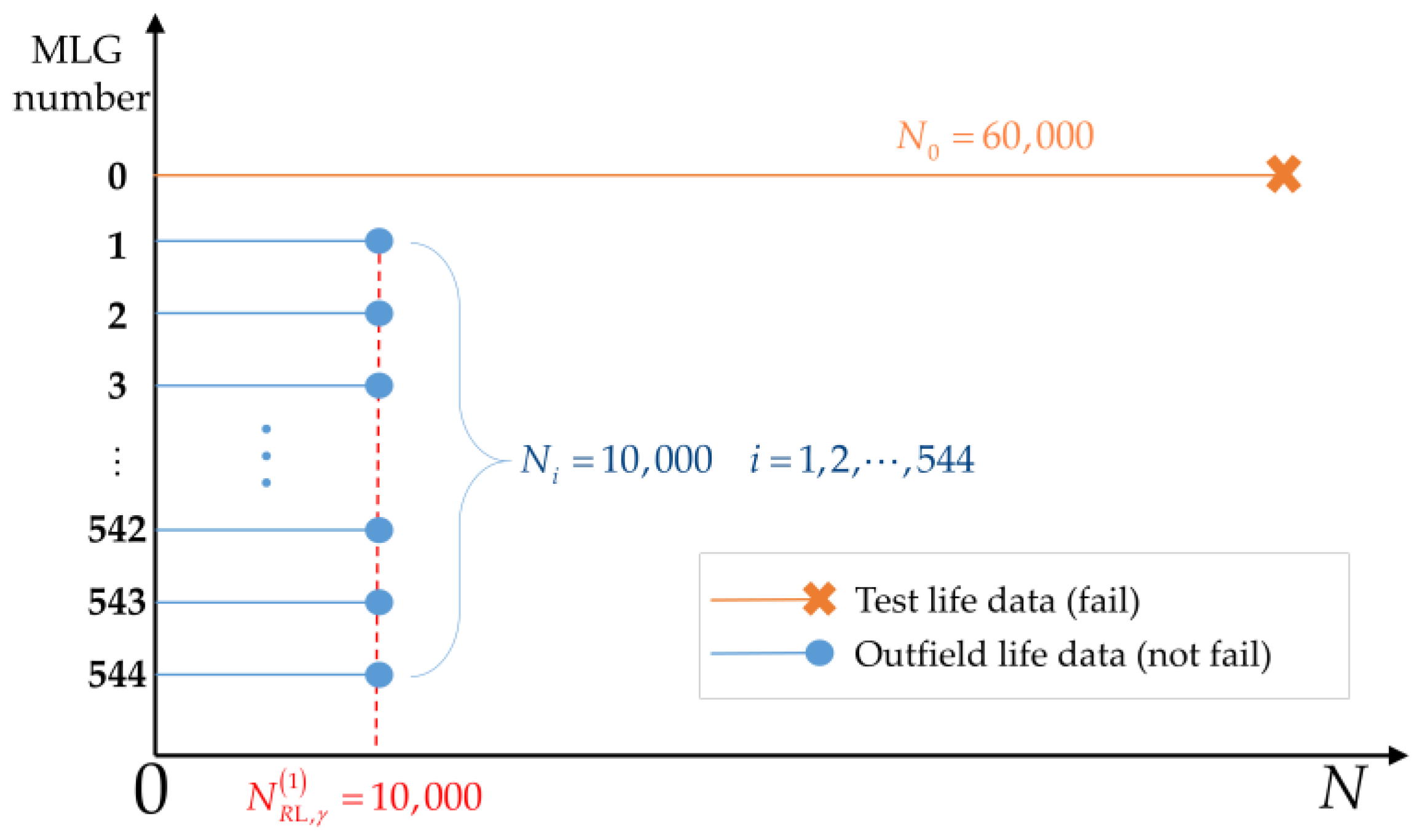
The life of a type of MLG follows a lognormal distribution. One landing gear sample was applied for the full-scale fatigue life test before delivery with the fatigue life of 60,000 flight cycles. With a fatigue scatter factor of , confidence of , and reliability of , the MLG’s safe life was determined via Equation (1) as
A total of 272 aircraft of this type are in service, and all the aircraft do not fail with the service time of 10,000 flight cycles. With two MLGs equipped in each aircraft, n = 544 outfield service life data were accumulated. The MLG’s test and outfield service data are plotted in Figure 4. Then, the MLG’s safe life in Equation (20) could be prolonged by the proposed safe life extension method in Section 2.2. The specific process and results were as follows.
Firstly, based on the MLG’s outfield data and Equations (8)–(12), the confidence of the 10,000 was updated from to . In the equations, can be found in Table 1, and the numerical precision parameter was set as .
Then, we adjusted the value of in Equation (12) to 0.8114. In this case, the calculation result of in Equation (8) was 0.90.
So, the lower confidence limit of the MLG’s reliable life with confidence and reliability was updated from 10,000 to , where
The MLG’s safe life was prolonged by 1173 flight cycles. The life extension percentage was
The above result indicated that the proposed method significantly prolonged the MLG’s safe life via numerous outfield data. In addition, life extension costs could be greatly reduced by avoiding additional life tests.
In engineering practice, the MLG’s safe life can be further extended with the continued service of the above MLGs. In this case, the new outfield life data will contain more statistical inference information. Therefore, the safe life extension effect will be more significant. For instance, if the n = 544 MLGs have all reached the extended safe life of 11,773 flight cycles in Equation (22) but still do not fail, then the MLG’s safe life can be extended to 12,885 flight cycles via the proposed method. Then, if the n = 544 MLGs have all reached the 12,885 flight cycles but still do not fail, the MLG’s safe life can be extended to 13,644 flight cycles. The specific process will not be repeated here.
4. Simulation Verification for MLG’s Safe Life Extension
The MLG’s safe life extension method in Section 2.2 was obtained by rigorous derivation. This section further verifies the method’s correctness via the simulation of the MLG’s safe life determination and extension process.
In the MLG’s life determination and extension, the safe life or calculated with the sample data (test life data or outfield life data) should be less than the actual value of reliable life . However, the and are both random variables since the sample data are random, so they cannot be guaranteed to be less than with a probability of 100%. Therefore, the probability of or is required to be for safety consideration in engineering practice. That is, the in Equation (1) and in Section 2.2 should satisfy
and
The above is the meaning of the confidence in the MLG’s safe life. The verification of the above probabilities is essential.
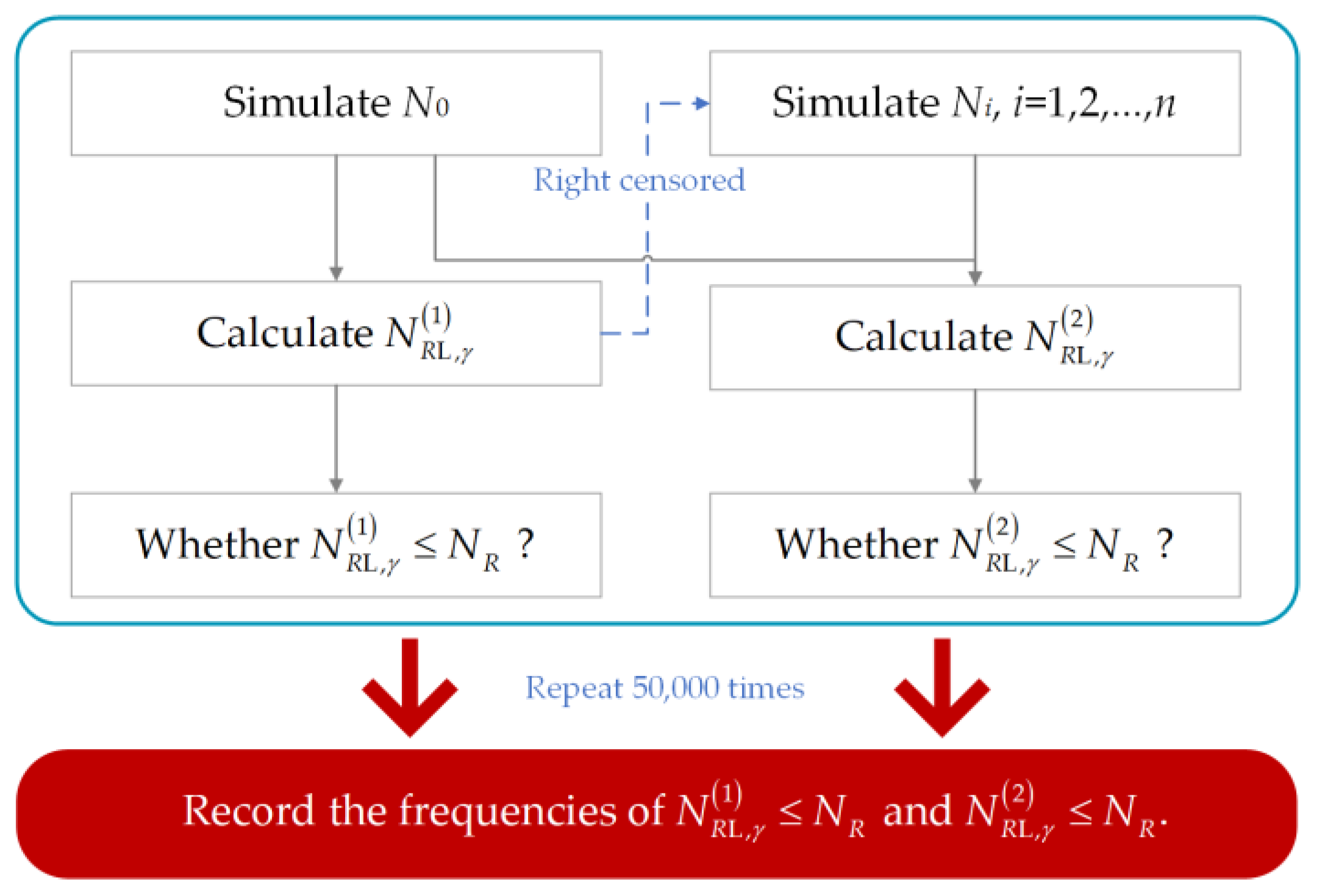
This section adopted the widely recognized Monte Carlo (MC) technology [32,33,34] to simulate the MLG’s safe life determination and extension process. In the simulations, the actual value of the MLG’s reliable life was known, so the determined and extended safe life could be compared with the reliable life to verify the correctness of Equations (24) and (25). The specific simulation steps are as follows.
Assume that the MLG’s logarithmic life follows a normal distribution with mean parameter and standard deviation parameter . That is, . Since the values of and are known, the actual value of the MLG’s reliable life can be calculated as
Then:
- (1)
- Randomly simulate the MLG’s full-scale fatigue life test data via MC;
- (2)
- Determine the MLG’s safe life using the test life and Equation (1);
- (3)
- Randomly simulate the MLG’s outfield life data , , which should be censored at the determined safe life to match the engineering practice;
- (4)
- Extend the MLG’s safe life to via the proposed safe life extension method in Section 2.2;
- (5)
- Judge and record whether and are less than ;
- (6)
- Repeat Steps 1–5 50,000 times and count the frequencies of and in the MC simulations. That is, record the coverage probability for safe life determination and for safe life extension.
The above simulation process is summarized in Figure 5. The simulation parameters are set in Table 2 with the consideration of the possible circumstances in engineering practice. Among them, the MLG’s outfield amount is set as 200, 500, or 1000 to reflect the small, medium, or large service numbers for different aircraft types. The value of in the simulation can be found in Table 1.
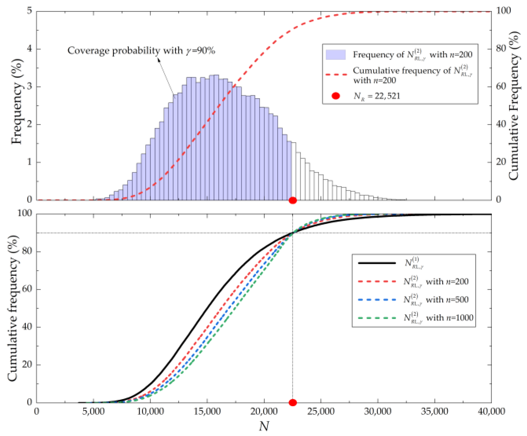
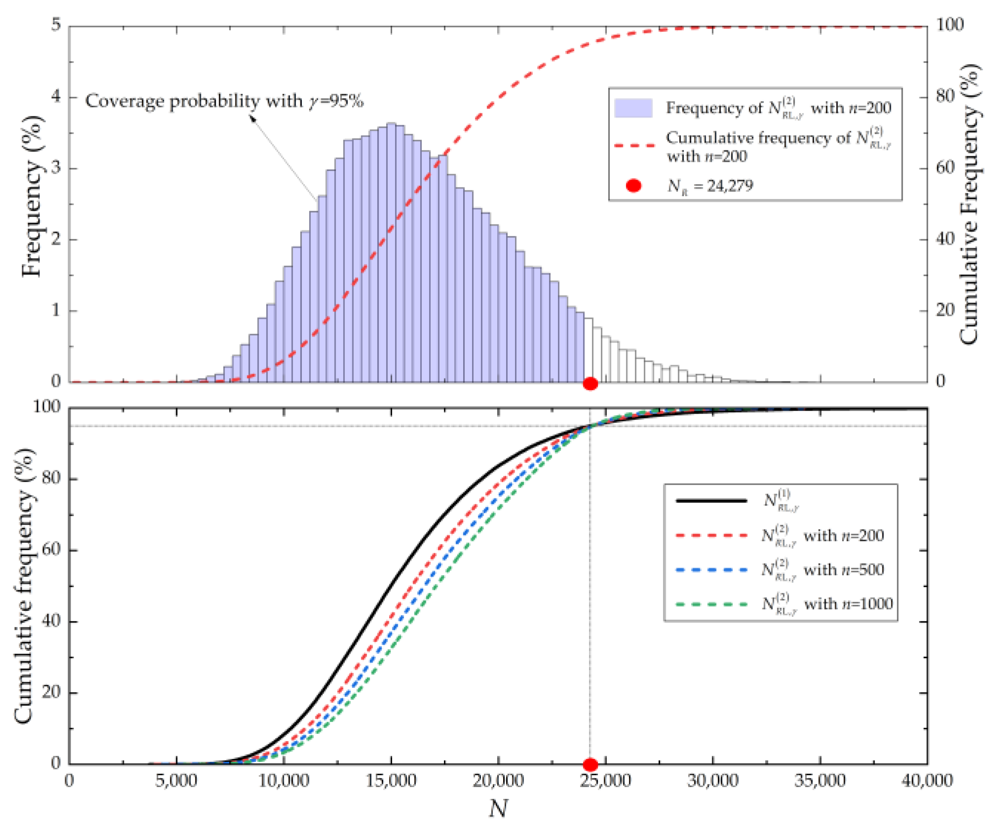
Figure 6 and Figure 7 illustrate the simulation results of the MLG’s safe life determination and extension in Simulation No. 1 and No. 2, respectively. In the figures, the block represents the frequency of () in 50,000 MC simulations. The black solid line, red dotted line, blue dotted line, and green dotted line represent the cumulative frequencies of , (), (), () in 50,000 MC simulations, respectively. It could be found that although the values of and were different, and could be both guaranteed with the required confidence (0.90 in Figure 6 and 0.95 in Figure 7). The above results proved the correctness of the proposed method.
For Simulations No. 1–No. 6, the coverage probabilities for safe life determination and for safe life extension are summarized in Table 3. The results indicated that both and were extremely close to under all simulation situations, which verified the correctness of Equations (24) and (25).
The was easily proved to be equal to in mathematics. However, fluctuating errors between and still existed, and they had the same size with fluctuating errors between and . In fact, the above fluctuating errors were caused by the MC simulation time limit (50,000 times). The errors could be reduced to zero by increasing the MC simulation times.
In addition, the mean value of the MLG’s logarithmic life was set as in the simulations, and the reliability was set as 0.999. The simulation verification results were the same for other values of and . These will not be repeated in this paper.
5. Conclusions
This paper proposed a novel method to prolong the MLG’s safe life. It could fully develop the MLG’s test life data and numerous outfield life data for statistical inference. Consequently, the MLG’s safe life estimated via only one fatigue test before delivery was prolonged to a new value. The provided example indicated that the proposed method achieved a significant effect with a safe life extension percentage of 17.73%, and the method will be more effective with the MLGs’ continued service after safe life extension. In addition, numerous simulations indicated that the extended safe life could always meet the requirements of reliability and confidence, demonstrating the method’s correctness. The advantage of this method is that it avoids additional fatigue tests required in traditional life extension methods. Thus, it can greatly reduce the life extension cost, which is significant in engineering practice.
The lognormal life distribution case was detailed in this paper, while the two-parameter Weibull life distribution is also commonly used for landing gear and other components. Similar to the lognormal distribution, the two-parameter Weibull distribution also presents a right-skewed asymmetric property on the image of the probability density function. Thus, we will further focus on safe life extension with the two-parameter Weibull distribution in the future. It is significant in engineering and also beneficial to symmetry research work.
Author Contributions
Conceptualization, Y.F. and H.F.; methodology, Y.F. and H.F.; software, Y.F.; validation, Y.F., H.F. and S.Z.; formal analysis, Y.F. and H.F.; investigation, Y.F. and H.F.; resources, Y.F., H.F. and S.Z.; data curation, Y.F.; writing—original draft preparation, Y.F.; writing—review and editing, Y.F., H.F. and S.Z.; visualization, Y.F.; supervision, S.Z.; project administration, H.F.; funding acquisition, H.F. All authors have read and agreed to the published version of the manuscript.
Funding
This research was funded by the National Natural Science Foundation of China (grant number U2037602).
Data Availability Statement
The data are contained within the article.
Acknowledgments
The authors gratefully acknowledge the financial support for this project from the National Natural Science Foundation of China (grant number U2037602).
Conflicts of Interest
The authors declare no conflict of interest.
Appendix A. The Confidence Updating Process Derivation of Equations (8)–(12)
This appendix provides the derivation of Equations (8)–(12).
Firstly, the fiducial distribution [35,36,37] of the MLG’s logarithmic reliable life is constructed according to the test data . Its probability density function and cumulative distribution function are expressed as
In the fiducial inference, . Denote event = {}, and is its opposing event. Then, the following can be derived:
Secondly, denote = {r MLGs fail with logarithmic life of , and n − r MLGs do not fail with logarithmic life of }. Then, the probability that events A and B occur simultaneously and the probability that events and B occur simultaneously can be calculated as
In the equations, is constant; is the mean parameter of the MLG’s logarithmic life distribution; and and are the probability density function and cumulative distribution function of , respectively.
Finally, when event B occurs (i.e., the MLG’s outfield service life data are generated), the probability of event A (i.e., the confidence of ) can be updated from to according to the following Bayesian approach:
In the equation, the value of is the updated confidence of . After substituting Equations (A1)–(A6) into Equation (A7), we get
In fact, Equations (8)–(12) provide the numerical solution of . A detailed explanation is given below.
Let and , then Equation (A8) can be transported to
Equally divide the interval (0, 1) into M parts and the interval (0, γ) into q = Mγ parts, then
can be calculated by the numerical integration as
So, the confidence updating process of Equations (8)–(12) is demonstrated.
Appendix B. The Mathematical Proof of Equations (18) and (19)
When the MLG’s outfield life data are all failure data (r = n), Equation (A8) can be transformed to
According to the updating process in Section 2.2, the aim is to find to satisfy
Thus:
and
So, the mathematical proof of Equations (18)–(19) is accomplished.
References
- Yan, C.L.; Liu, K.G. Theory of Economic Life Prediction and Reliability Assessment of Aircraft Structures. Chin. J. Aeronaut. 2011, 24, 164–170. [Google Scholar] [CrossRef] [Green Version]
- Aftab, S.G.; Sirajuddin; Sreedhara, B.; Ganesh, E.; Babu, N.R.; Aithal, S.K. Finite Element Analysis of a Passenger Aircraft Landing Gear for Structural and Fatigue Safety. Mater. Today Proc. 2022, 54, 152–158. [Google Scholar] [CrossRef]
- Bagnoli, F.; Dolce, F.; Colavita, M.; Bernabei, M. Fatigue Fracture of a Main Landing Gear Swinging Lever in a Civil Aircraft. Eng. Fail. Anal. 2008, 15, 755–765. [Google Scholar] [CrossRef]
- Franco, L.A.L.; Lourenco, N.J.; Graca, M.L.A.; Silva, O.M.M.; de Campos, P.P.; von Dollinger, C.F.A. Fatigue Fracture of a Nose Landing Gear in a Military Transport Aircraft. Eng. Fail. Anal. 2006, 13, 474–479. [Google Scholar] [CrossRef]
- Xue, C.J.; Dai, J.H.; Wei, T.; Liu, B.; Deng, Y.Q.; Ma, J. Structural Optimization of a Nose Landing Gear Considering Its Fatigue Life. J. Aircr. 2012, 49, 225–236. [Google Scholar] [CrossRef]
- Insley, J.; Turkoglu, C. A Contemporary Analysis of Aircraft Maintenance-Related Accidents and Serious Incidents. Aerospace 2020, 7, 81. [Google Scholar] [CrossRef]
- Yan, C.L.; Su, K.X. Design of Safe Life and Damage Tolerance for Aircraft Landing Gear; Aviation Industry Press: Beijing, China, 2011; ISBN 978-7-80243-894-1. (In Chinese) [Google Scholar]
- Tao, J.X.; Smith, S.; Duff, A. The Effect of Overloading Sequences on Landing Gear Fatigue Damage. Int. J. Fatigue 2009, 31, 1837–1847. [Google Scholar] [CrossRef]
- Grandt, F., Jr. Damage Tolerant Design and Nondestructive Inspection—Keys to Aircraft Airworthiness. Procedia Eng. 2011, 17, 236–246. [Google Scholar] [CrossRef] [Green Version]
- Tavares, S.M.O.; De Castro, P.M.S.T. An Overview of Fatigue in Aircraft Structures. Fatigue Fract. Eng. Mater. Struct. 2017, 40, 1510–1529. [Google Scholar] [CrossRef]
- Tuegel, E.J.; Bell, R.P.; Berens, A.P.; Brussat, T.; Cardinal, J.W.; Gallagher, J.P.; Rudd, J. Aircraft Structural Reliability and Risk Analysis Handbook Volume 1: Basic Analysis Methods; Air Force Research Laboratory Headquarters: Wright-Patterson AFB, OH, USA, 2013; pp. 1–104. [Google Scholar]
- Glista, S.M.; Postema, W.; Arcusa, L.; Clark, B. F-22 MECSIP Lessons Learned: Risk Based Fatigue Scatter Factors High Durability Margin Analysis Using Miner’s Rule and Weibull Analysis. In Proceedings of the ASME 2011 International Mechanical Engineering Congress & Exposition; ASMEDC: Denver, CO, USA, 2011; pp. 593–610. [Google Scholar] [CrossRef]
- Brot, A. Weibull or Log-Normal Distribution to Characterize Fatigue Life Scatter—Which Is More Suitable? In Proceedings of the ICAF 2019—Structural Integrity in the Age of Additive Manufacturing; Niepokolczycki, A., Komorowski, J., Eds.; Springer International Publishing: Cham, Switzerland, 2020; pp. 551–561. [Google Scholar] [CrossRef]
- Brady, J.F. Maintenance Reliability Analysis for Increasing Parts Availability and Reducing Operations and Maintenance Costs. Ph.D. Thesis, The George Washington University, Washington, DC, USA, 2019. [Google Scholar]
- Dziendzikowski, M.; Kurnyta, A.; Reymer, P.; Kurdelski, M.; Klysz, S.; Leski, A.; Dragan, K. Application of Operational Load Monitoring System for Fatigue Estimation of Main Landing Gear Attachment Frame of an Aircraft. Materials 2021, 14, 6564. [Google Scholar] [CrossRef]
- Ball, D.L.; Gross, P.C.; Burt, R.J. F-35 Full Scale Durability Modeling and Test. Adv. Mater. Res. 2014, 891–892, 693–701. [Google Scholar] [CrossRef]
- Sawaisarje, G.; Khapli, R.P. Fatigue Crack Growth (FCG) Studies on Landing Gear (LG) Actuating Cylinder of Fighter Aircraft for Life Extension. In Proceedings of the Fatigue, Durability, and Fracture Mechanics; Seetharamu, S., Jagadish, T., Malagi, R., Eds.; Springer Singapore: Singapore, 2021; pp. 53–62. [Google Scholar]
- Yan, C.L.; Liu, K.G. Fatigue Scatter Factor of Whole Life and Reliability of Aircraft Structure Service Life. Adv. Mater. Res. 2008, 44–46, 739–744. [Google Scholar] [CrossRef]
- General Armament Department of the People’s Liberation Army of China. GJB 67.6A-2008; Military Airplane Structural Strength Specification Part6: Repeated Loads, Durability and Damage Tolerance. General Equipment Department Military Standard Publishing and Distribution Department: Beijing, China, 2008. (In Chinese)
- Chen, Z.W. Structural Reliable Life and Spectrum Difference Factor. Int. J. Fatigue 1993, 15, 389–391. [Google Scholar] [CrossRef]
- Skorupka, Z.; Tywoniuk, A. Health Monitoring in Landing Gears. J. KONES Powertrain Transp. 2019, 26, 167–174. [Google Scholar] [CrossRef] [Green Version]
- Pfingstl, S.; Steinweg, D.; Zimmermann, M.; Hornung, M. On the Potential of Extending Aircraft Service Time Using Load Monitoring. J. Aircr. 2022, 59, 377–385. [Google Scholar] [CrossRef]
- Skorupka, Z. Dynamic Fatigue Tests of Landing Gears. Fatigue Aircr. Struct. 2020, 2020, 69–77. [Google Scholar] [CrossRef]
- Zhuo, N.S.; Fu, Y.Z.; Hu, Z. Summary of determination of structures fatigue life for Y8 aircraft series. Aeronaut. Sci. Technol. 2006, 2006, 40–44. (In Chinese) [Google Scholar] [CrossRef]
- Iele, A.; Leone, M.; Consales, M.; Persiano, G.V.; Brindisi, A.; Ameduri, S.; Concilio, A.; Ciminello, M.; Apicella, A.; Bocchetto, F.; et al. Load Monitoring of Aircraft Landing Gears Using Fiber Optic Sensors. Sens. Actuators Phys. 2018, 281, 31–41. [Google Scholar] [CrossRef]
- Holmes, G.; Sartor, P.; Reed, S.; Southern, P.; Worden, K.; Cross, E. Prediction of Landing Gear Loads Using Machine Learning Techniques. Struct. Health Monit.-Int. J. 2016, 15, 568–582. [Google Scholar] [CrossRef]
- Wang, S.Y.; Gui, W.H. Corrected Maximum Likelihood Estimations of the Lognormal Distribution Parameters. Symmetry 2020, 12, 968. [Google Scholar] [CrossRef]
- Bazaras, Z.; Lukosevicius, V. Statistical Assessment of Low-Cycle Fatigue Durability. Symmetry 2022, 14, 1205. [Google Scholar] [CrossRef]
- Nuti, A.; Bertini, F.; Cipolla, V.; Di Rito, G. Design of a Fuselage-Mounted Main Landing Gear of a Medium-Size Civil Transport Aircraft. Aerotec. Missili Spaz. 2018, 97, 85–95. [Google Scholar] [CrossRef] [Green Version]
- Lin, X.; Cai, B.; Wang, L.; Zhang, Z. A Bayesian Proportional Hazards Model for General Interval-Censored Data. Lifetime Data Anal. 2015, 21, 470–490. [Google Scholar] [CrossRef] [PubMed]
- Chen, W.B.; Li, X.Y.; Li, F.R.; Kang, R. Belief Reliability Evaluation with Uncertain Right Censored Time-to-Failure Data under Small Sample Situation. Qual. Reliab. Eng. Int. 2022, 38, 3099–3115. [Google Scholar] [CrossRef]
- Balakrishnan, N.; Ling, M.H. Gamma Lifetimes and One-Shot Device Testing Analysis. Reliab. Eng. Syst. Saf. 2014, 126, 54–64. [Google Scholar] [CrossRef]
- Zhang, C.W. Weibull Parameter Estimation and Reliability Analysis with Zero-Failure Data from High-Quality Products. Reliab. Eng. Syst. Saf. 2021, 207, 107321. [Google Scholar] [CrossRef]
- Singh, D.P.; Lodhi, C.; Tripathi, Y.M.; Wang, L. Inference for Two-Parameter Rayleigh Competing Risks Data under Generalized Progressive Hybrid Censoring. Qual. Reliab. Eng. Int. 2021, 37, 1210–1231. [Google Scholar] [CrossRef]
- Hannig, J.; Iyer, H.; Lai, R.C.S.; Lee, T.C.M. Generalized Fiducial Inference: A Review and New Results. J. Am. Stat. Assoc. 2016, 111, 1346–1361. [Google Scholar] [CrossRef]
- Xie, M.; Singh, K. Confidence Distribution, the Frequentist Distribution Estimator of a Parameter: A Review. Int. Stat. Rev. 2013, 81, 3–39. [Google Scholar] [CrossRef]
- Qi, X.L.; Li, H.H.; Tian, W.Z.; Yang, Y.T. Confidence Interval, Prediction Interval and Tolerance Interval for the Skew Normal Distribution: A Pivotal Approach. Symmetry 2022, 14, 855. [Google Scholar] [CrossRef]
Figure 1.
The schematic diagram of the MLG’s safe life extension method.

Figure 2.
The schematic diagram of the MLG’s outfield service life data.

Figure 3.
Updating process for the lower confidence limit of the MLG’s logarithmic reliable life.

Figure 4.
Test life data and outfield life data of the MLG.

Figure 5.
Simulation process of the MLG’s safe life determination and extension.

Figure 6.
Simulation results of the MLG’s safe life determination and extension in Simulation No. 1 (Lf = 4.0 and γ = 0.90).
Figure 6.
Simulation results of the MLG’s safe life determination and extension in Simulation No. 1 (Lf = 4.0 and γ = 0.90).

Figure 7.
Simulation results of the MLG’s safe life determination and extension in Simulation No. 2 (Lf = 4.0 and γ = 0.95).
Figure 7.
Simulation results of the MLG’s safe life determination and extension in Simulation No. 2 (Lf = 4.0 and γ = 0.95).


Table 1.
The relationship between Lf and σ0 for the main landing gear (MLG) with R = 0.999.
| Scatter factor Lf | 4.0 | 4.0 | 5.0 | 5.0 | 6.0 | 6.0 |
| Confidence γ | 0.90 | 0.95 | 0.90 | 0.95 | 0.90 | 0.95 |
| Standard deviation σ0 | 0.138 | 0.127 | 0.160 | 0.148 | 0.178 | 0.164 |
Table 2.
Simulation parameters in the MLG’s safe life determination and extension simulation (μ = lg 60,000; R = 0.999).
Table 2.
Simulation parameters in the MLG’s safe life determination and extension simulation (μ = lg 60,000; R = 0.999).
| Simulation No. | Scatter Factor Lf | Required Confidence γ | Outfield Amount n |
|---|---|---|---|
| 1 | 4.0 | 0.90 | 200, 500, 1000 |
| 2 | 4.0 | 0.95 | |
| 3 | 5.0 | 0.90 | |
| 4 | 5.0 | 0.95 | |
| 5 | 6.0 | 0.90 | |
| 6 | 6.0 | 0.95 |
Table 3.
Simulation verifications of the MLG’s safe life determination and extension.
| Simulation No. | Scatter Factor Lf | Required Confidence γ | Coverage Probability γ(1) | Respective Coverage Probabilities γ(2) with n = 200, 500, 1000 |
|---|---|---|---|---|
| 1 | 4.0 | 0.90 | 0.899 | 0.899, 0.899, 0.900 |
| 2 | 4.0 | 0.95 | 0.950 | 0.949, 0.950, 0.950 |
| 3 | 5.0 | 0.90 | 0.900 | 0.899, 0.899, 0.898 |
| 4 | 5.0 | 0.95 | 0.949 | 0.950, 0.950, 0.950 |
| 5 | 6.0 | 0.90 | 0.898 | 0.900, 0.901, 0.898 |
| 6 | 6.0 | 0.95 | 0.951 | 0.951, 0.949, 0.949 |
Disclaimer/Publisher’s Note: The statements, opinions and data contained in all publications are solely those of the individual author(s) and contributor(s) and not of MDPI and/or the editor(s). MDPI and/or the editor(s) disclaim responsibility for any injury to people or property resulting from any ideas, methods, instructions or products referred to in the content. |
© 2023 by the authors. Licensee MDPI, Basel, Switzerland. This article is an open access article distributed under the terms and conditions of the Creative Commons Attribution (CC BY) license (https://creativecommons.org/licenses/by/4.0/).
Share and Cite
MDPI and ACS Style
Fu, Y.; Fu, H.; Zhang, S. A Novel Safe Life Extension Method for Aircraft Main Landing Gear Based on Statistical Inference of Test Life Data and Outfield Life Data. Symmetry 2023, 15, 880. https://doi.org/10.3390/sym15040880
AMA Style
Fu Y, Fu H, Zhang S. A Novel Safe Life Extension Method for Aircraft Main Landing Gear Based on Statistical Inference of Test Life Data and Outfield Life Data. Symmetry. 2023; 15(4):880. https://doi.org/10.3390/sym15040880
Chicago/Turabian StyleFu, Yueshuai, Huimin Fu, and Sheng Zhang. 2023. "A Novel Safe Life Extension Method for Aircraft Main Landing Gear Based on Statistical Inference of Test Life Data and Outfield Life Data" Symmetry 15, no. 4: 880. https://doi.org/10.3390/sym15040880
Note that from the first issue of 2016, this journal uses article numbers instead of page numbers. See further details here.