
Survival Analysis and Applications of Weighted NH Parameters Using Progressively Censored Data


1
Faculty of Technology and Development, Zagazig University, Zagazig 44519, Egypt
2
Department of Mathematical Sciences, College of Science, Princess Nourah bint Abdulrahman University, P.O. Box 84428, Riyadh 11671, Saudi Arabia
*
Author to whom correspondence should be addressed.
Symmetry 2023, 15(3), 735; https://doi.org/10.3390/sym15030735
Submission received: 29 January 2023
/
Revised: 11 March 2023
/
Accepted: 13 March 2023
/
Published: 15 March 2023
(This article belongs to the Special Issue Mathematical Models and Methods in Various Sciences)
Abstract
:A new weighted Nadarajah–Haghighi (WNH) distribution, as an alternative competitor model to gamma, standard half-logistic, generalized-exponential, Weibull, and other distributions, is considered. This paper explores both maximum likelihood and Bayesian estimation approaches for estimating the parameters, reliability, and hazard rate functions of the WNH distribution when the sample type is Type-II progressive censored order statistics. In the classical interval setup, both asymptotic and bootstrap intervals of each unknown parameter are constructed. Using independent gamma priors and symmetric squared-error loss, the Bayes estimators cannot be obtained theoretically. Thus, two approximation techniques, namely: Lindley and Markov-Chain Monte Carlo (MCMC) methods, are used. From MCMC variates, the Bayes credible and highest posterior density intervals of all unknown parameters are also created. Extensive Monte Carlo simulations are implemented to compare the performance of the proposed methodologies. Numerical evaluations showed that the estimates developed by the MCMC sampler performed better than the Lindley estimates, and both behaved significantly better than the frequentist estimates. To choose the optimal censoring scheme, several optimality criteria are considered. Three engineering applications, including vehicle fatalities, electronic devices, and electronic components data sets, are provided. These applications demonstrated how the proposed methodologies could be applied in real practice and showed that the proposed model provides a satisfactory fit compared to three new weighted models, namely: weighted exponential, weighted Gompertz, and new weighted Lindley distributions.
1. Introduction
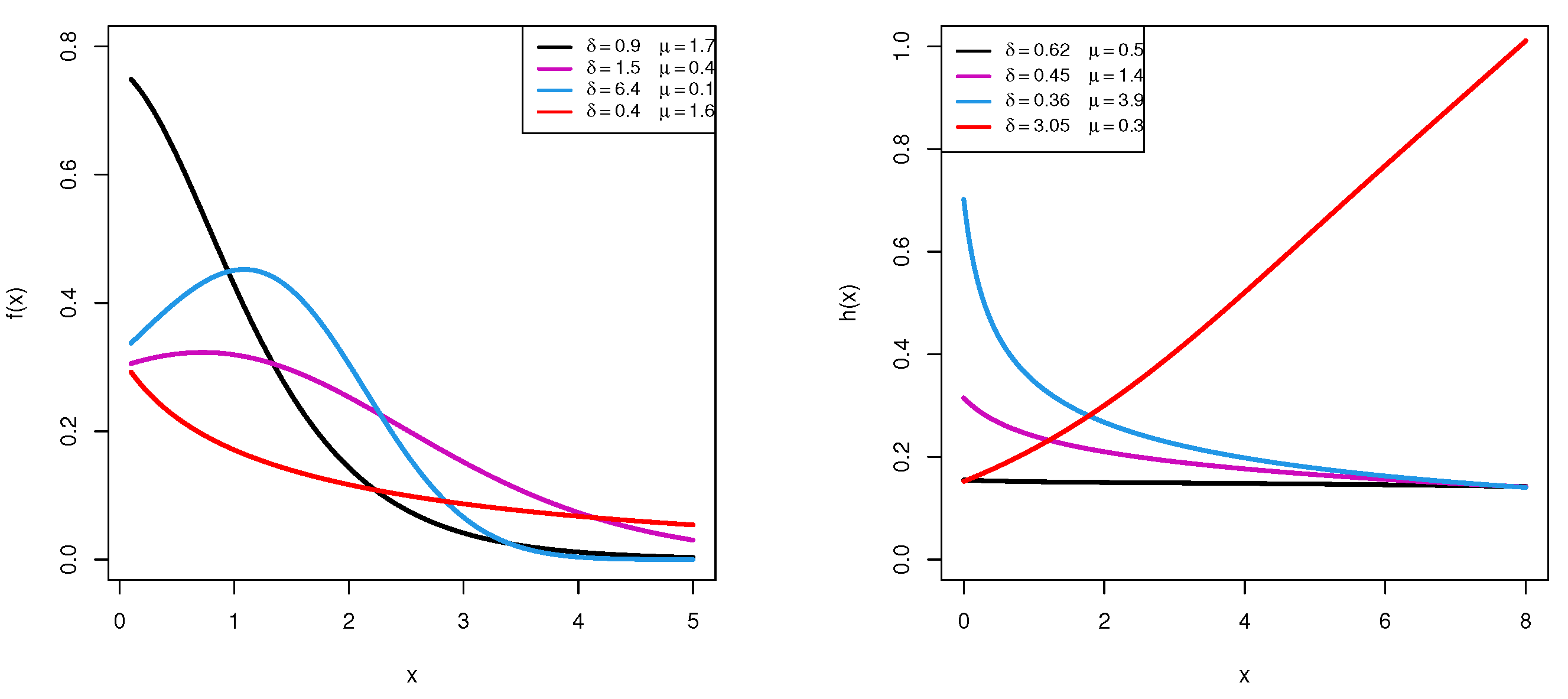
The Nadarajah–Haghighi (NH) distribution, proposed by Nadarajah and Haghighi [1], has a density shape that can be growing or unimodal as well as a hazard rate that can be increasing, decreasing, or constant. Recently, as a new weighted version of the NH distribution, according to the idea of created weighted distributions, Khan et al. [2] proposed the weighted Nadarajah–Haghighi (WNH) distribution as a competitive model to other lifetime models, such as gamma, exponentiated half-logistic, generalized-exponential, Weibull, etc. They also stated that the WNH distribution is suitable for modeling data from different areas; for example, reliability, survival analysis, forest, ecological, etc. Suppose that X is a lifetime random variable of the test unit(s) following the two-parameter distribution. Then, its probability density function (PDF) and cumulative distribution function (CDF) are given, respectively, as
and
where and are the shape and scale parameters, respectively. From (1), Khan et al. [2] showed that the WNH distribution could be considered an extended model of three common distributions, namely: NH, standard half-logistic and zero truncated weighted Weibull models, such as:
- Nadarajah–Haghighi distribution by multiplying (1) by .
- Standard half-logistic distribution by setting .
- Truncated weighted Weibull by setting .
Further, the reliability function (RF) and hazard function (HF) at distinct time t are
and
respectively. From (2), where , two lifetime models can be obtained by making a useful transformation, namely (i) standard half-logistic distribution when and (ii) zero truncated weighted Weibull distribution when . Figure 1 depicts the density and hazard rate shapes of the distribution for several choices of its parameters. It reveals that the PDF (1) is positively skewed while the HF (4) has increasing, decreasing, and constant shapes.
In the past decade, researchers have favored dealing with progressive Type-II censoring (PCTII) over other censoring mechanisms because it (i) reduces the total testing time, (ii) reduces the cost of failed units, (iii) terminates the experiment rapidly, and (iv) allows the researcher to make use of the units removed during the experiment for use in other tests. Briefly, the PCTII can be described as: Suppose that n independent and identical units are subjected to a life-testing experiment at time zero, m is a fixed number of failures and the censoring scheme is also pre-specified. At the time that the first failure is observed (say ), survival units are randomly removed from the experiment. Following the second observed failure (say ), of survival units are randomly removed from units, and so on. This mechanism continues until the failure occurs and the experiment is stopped. At the same time, all remaining units are removed. Let be a PCTII sample of size m with censoring from a continuous population.
Then, the likelihood function of , where is the parameter vector, can be expressed as
where .
Various studies on the NH distribution using censored data have been made in the literature, readers may refer to Mohie El-Din et al. [3], Ashour et al. [4], Wu and Gui [5], Elshahhat et al. [6], Elshahhat and Abu El Azm [7], Dey et al. [8], Almarashi et al. [9], among others.
Although the NH distribution has received a lot of attention from several authors to the best of our knowledge, the problem of estimating the WNH parameters and/or the RF and HF via PCTII sampling has yet to be investigated. Therefore, this article offers an analysis of PCTII lifetime data when each test unit follows the WNH distribution. The maximum likelihood estimators (MLEs) with their Fisher information members are evaluated through the standard Newton–Raphson algorithm. The associated asymptotic normality of the MLE and log-MLE is used to construct the asymptotic confidence intervals (ACIs). Further, for all unknown quantities, bootstrap-p and bootstrap-t intervals are also obtained. Using the Lindley and Metropolis–Hastings (M-H) methods, the Bayes estimates against the squared-error loss (SEL) function can be easily approximated. Using Markov chain Monte Carlo (MCMC) steps, the Bayes credible interval (BCI) and the highest posterior density (HPD) interval for each unknown parameter are obtained. To compare two (or more) different progressive censoring plans, using their Fisher information, different optimality criteria are taken into account. To assess the performance of the proposed estimation methodologies, an extensive Monte Carlo simulation is performed. Lastly, three applications based on real-life engineering data are presented to show the superiority and flexibility of the WNH model over three weighted distributions (as competitors), namely: weighted exponential, weighted Gompertz, and weighted Lindley distributions. Additionally, the proposed applications aim to demonstrate the applicability of the acquired estimators in a real-life scenario.
The rest of the article is classified as: Section 2 provides the likelihood inference. Two kinds of bootstrapping are presented in Section 3. Bayes approximation techniques are discussed in Section 4. Simulation results are provided in Section 5. In Section 6, a brief explanation of the optimum progressive censoring is presented. Three real applications are presented in Section 7. In Section 8, some conclusions are offered.
2. Likelihood Inference
This section deals with finding the MLEs of the model parameters and the reliability characteristics of the WNH distribution based on PCTII data. Two-sided ACIs of the same unknown parameters are also obtained here.
2.1. Maximum Likelihood Estimators
Suppose , is a PCTII sample acquired from the WNH having a fixed . Substituting (1) and (2) into (5), where is used in the place of , we receive
where .
The log-likelihood function () of (6) can be expressed (up to proportional) as
Differentiating (7) partially with respect to and , two likelihood equations are obtained as
and
where is the first-partial derivative with respect to , such as
and for
It is observed, from (8) and (9), that the MLEs and are derived in a system of nonlinear equations. Thus, a suitable iterative procedure, such as the Newton–Raphson iterative method, is used. For this reason, the ‘’ package suggested by Henningsen and Toomet [10] is considered. Next, by replacing and with their MLEs and , respectively, the MLEs and can be easily derived.
2.2. Asymptotic Interval Estimators
To create the ACIs of , , , or , the variance-covariance (VCov) matrix of and must be obtained first as
where, from (7), the elements are obtained and presented in Appendix A.
Under certain regularity conditions, the asymptotic normality of is approximately distributed as bivariate normal . Thus, following the normal approximation (NA) of the MLEs and , two bounds ACI via NA (ACI-NA) of and can be obtained, respectively, by
where is the upper ()th probability point of the standard normal distribution.
Further, to obtain the ACIs of and , the delta method is used to approximate their variances, see Greene [11]. However, from the Fisher information (10), the approximated variances of and are given by
respectively, where and , such as
and
where .
Thus, at the confidence percent , the ACI-NA of and are obtained, respectively, as
where is the percentile of the standard normal distribution with right-tail probability .
In practice, the main problem with the ACI-NA method is that it may give a negative lower bound for a lifetime parameter. For handling this disadvantage, Meeker and Escobar [12] developed the normal log-transformed (NL) approximation for the MLE. They also stated that the ACI has the highest CP based on the NL compared to the other NA. Then, the ACI via NL (ACI-NL) of is given by
where, in a similar fashion, the other ACI-NL of , or can be easily computed.
3. Bootstrapping Estimators
If the sample size m is small, due to the law of large numbers, both ACIs developed by NA and NL methods cannot perform well. In this section, two bootstrapping techniques, namely: bootstrap-p and bootstrap-t algorithms, are obtained for , , , and . To obtain the bootstrap-p (or bootstrap-t) of , , or , we first need to receive a bootstrap sample, as shown in Algorithm 1.
| Algorithm 1 Bootstrap Sampling: |
|
Then, using the bootstrap-p and bootstrap-t methods, the bootstrap intervals of , , and can be constructed as
- (i)
- Bootstrap-p (Boot-p) Method: The % boot-p intervals of , , and (say ) are given, respectively, by
- (ii)
- Bootstrap-t (Boot-t) Method: The % boot-t intervals of , , and are given by
- 1.
- Define the T-statistic for , , and (say ) aswhere is the MLE of and is the observed estimated variance of .
- 2.
- Arrange the T-statistics as .
- 3.
- The % bootstrap-t interval of is given by
4. Bayes Estimators
The Bayes’ paradigm provides the possibility of incorporating prior information about the unknown parameter(s) of interest. To establish this method, the WNH parameters and are assumed to be random variables with some extra information included in their prior distributions. One of the most flexible priors is called the gamma conjugate density prior; see Kundu [13]. Gamma density is fairly straightforward and flexible enough to cover a large variety of the experimenter’s prior beliefs. We, therefore, assumed that and , having independent gamma PDFs as and , where are chosen to reflect prior knowledge about the parameters. Thus, the joint gamma PDF of and becomes
where and are assumed to be known. On the other hand, the most widely used loss is called the SEL function, , and is defined as
where denotes the Bayes estimate of .
From (12), the target Bayes estimate is given by the posterior expectation of . The joint posterior PDF, by combining (11) with (6), of and is
where . However, using (12), the Bayes estimator for any function of and , say is given by
It is clear, based on (14), that the Bayes estimate of is derived in an expression of the ratio of double integrals.
Then, the Bayes solution for each unknown parameter is not available. We, therefore, propose to use both the Lindley and MCMC methods to approximate the Bayes estimates.
4.1. Lindley’s Approximation
In this subsection, following Lindley [14], the closed expressions for the Bayes estimates are obtained. However, setting for simplicity, the approximated posterior expectation (say ) of is given by
where all terms in (15) are evaluated at their and , , , , , , , , , , , , and in the element of the VCov matrix (10).
From (15), the Lindley’s estimators and of and , respectively, as
and
where , , and the items (for ) are obtained and reported in Appendix B.
Similarly, using (15), the Lindley’s estimators of the reliability characteristic functions and of and are given (for ), respectively, by
and
where is given in Section 2.2 and of , and are obtained and presented in Appendix C.
Although the Lindley estimators of , , , and are expressed explicitly, the main problem of this approach is its disability to obtain an interval estimate. Consequently, to approximate the Bayes estimates and to construct their BCI and HPD interval estimates, the M-H algorithm is considered.
4.2. M-H Sampler
Since the joint posterior PDF cannot be reduced by analytical steps to any familiar form, the M-H algorithm (which is one of the effective MCMC techniques) is used, see Gelman et al. [15].
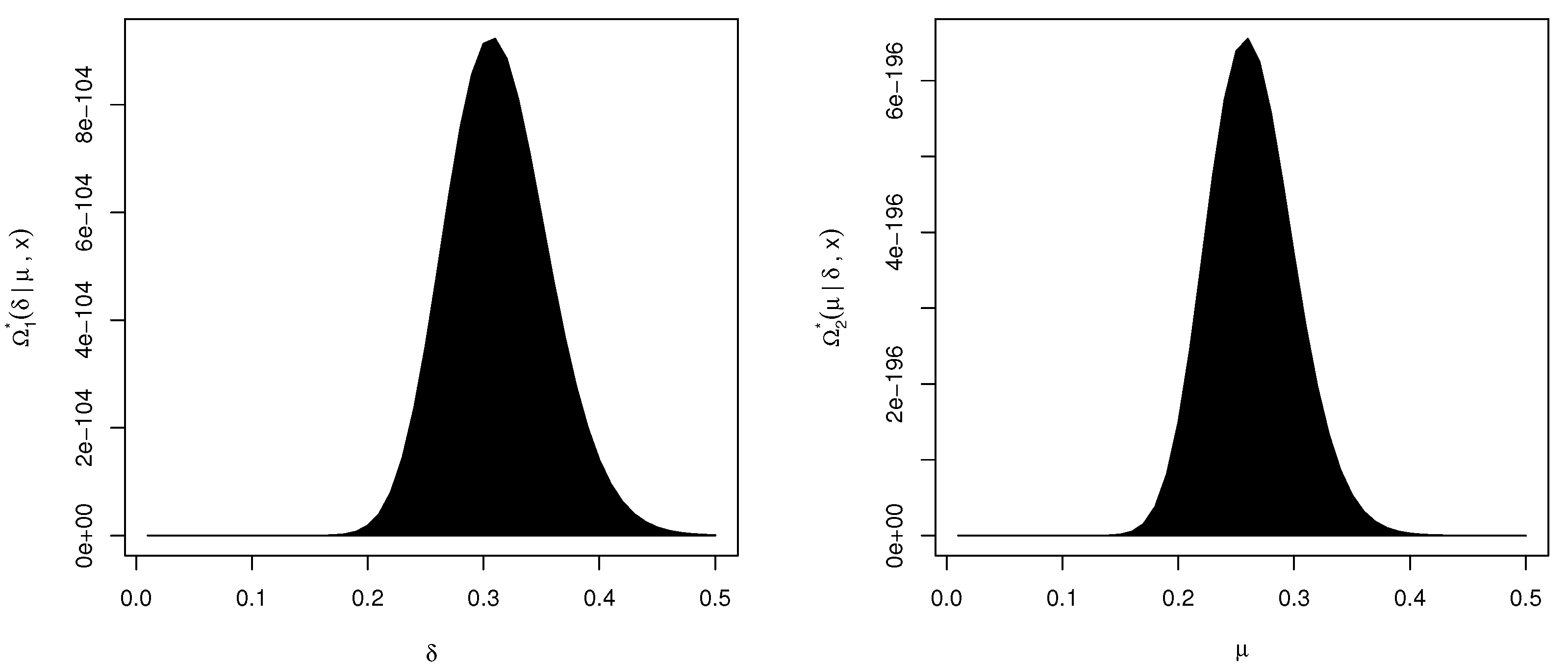
As we anticipated, the conditional distributions (16) and (17) of and , respectively, cannot be reduced to any standard distribution. Figure 2 shows that the distributions (16) and (17) behave like a normal density. Therefore, to obtain the Bayes MCMC estimates along with their BCI and HPD intervals, we perform the generation process described in Algorithm 2.
| Algorithm 2 Markov Chain Monte Carlo Sampling: |
|
5. Numerical Comparisons
To compare the efficiency of the proposed estimators of , , , and described in the preceding sections, based on 2000 PCTII samples generated from via Algorithm 3, an extensive Monte Carlo simulation is conducted. At distinct time , the corresponding actual values of and are taken as 0.935 and 0.012, respectively. Various combinations of the total sample size n and effective sample size m are also considered, such as , and m is taken as 50% and 80% for each n. Three different progressive designs, where means that 0 is repeated times, are used, namely:
To draw a PCTII sample from the WNH distribution for pre-specified values of n, m, and , we perform the following steps:
| Algorithm 3 Progressive Type-II Censored Sampling: |
|
Using each simulated sample, the point estimators, such as maximum likelihood, Lindley, and MCMC, are compared using their mean absolute bias (MAB), and root mean squared error (RMSE) simulated values. Further, the 95% interval estimators, called ACI-NA, ACI-NL, Boot-p, Boot-t, BCI, and HPD intervals, are examined via their simulated average confidence length (ACL) and coverage probability (CP) values. Following Algorithm 1, the bootstrapping procedure of , , , and is repeated 10,000 times.
To compute the Bayes estimates and BCI/HPD intervals of , , , or , we repeat Algorithm 2 12,000 times and ignore the first 2000 times as burn-in. For both WNH parameters and , two different informative sets of the hyperparameters are used, namely: Prior-1 (P1): and Prior-2 (P2): . These prior sets are specified based on two criteria called prior mean and prior variance in such a way that the prior mean becomes the plausible value of the corresponding unknown parameter. All numerical computations are carried out via 4.1.2 software utilizing two recommended packages, namely: ‘’ and ‘’ packages, as suggested by Plummer et al. [16] and Henningsen and Toomet [10], respectively.
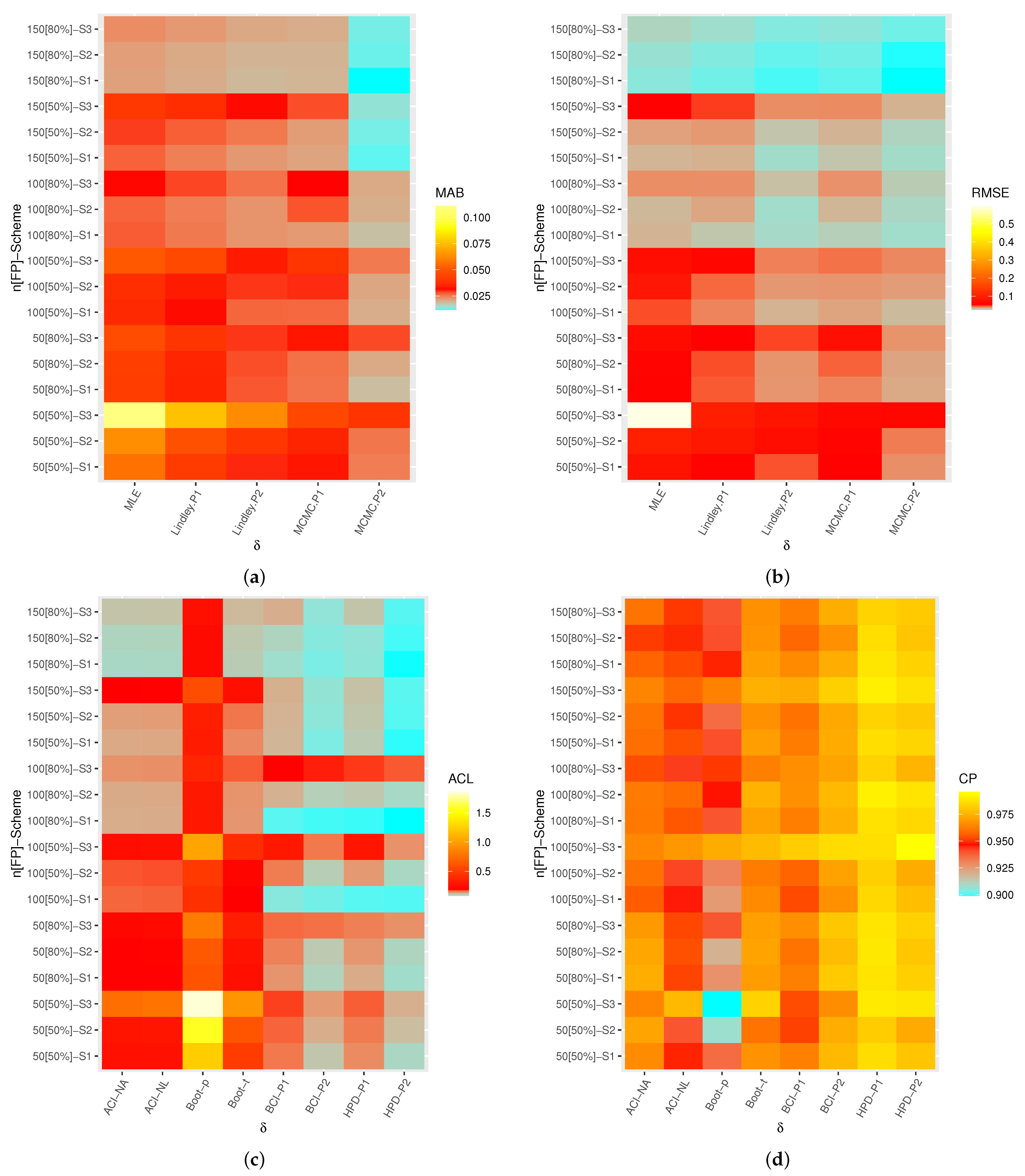
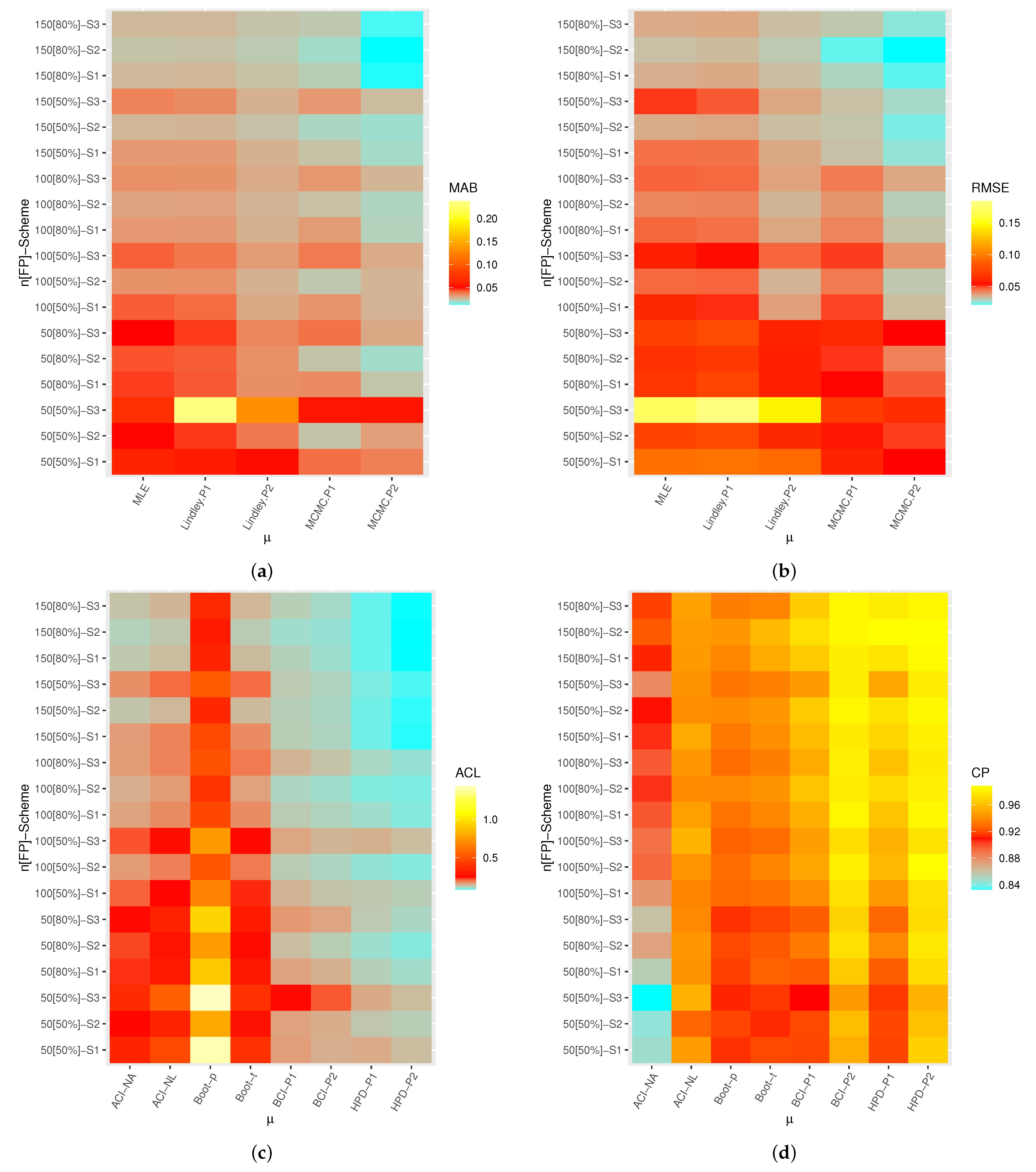
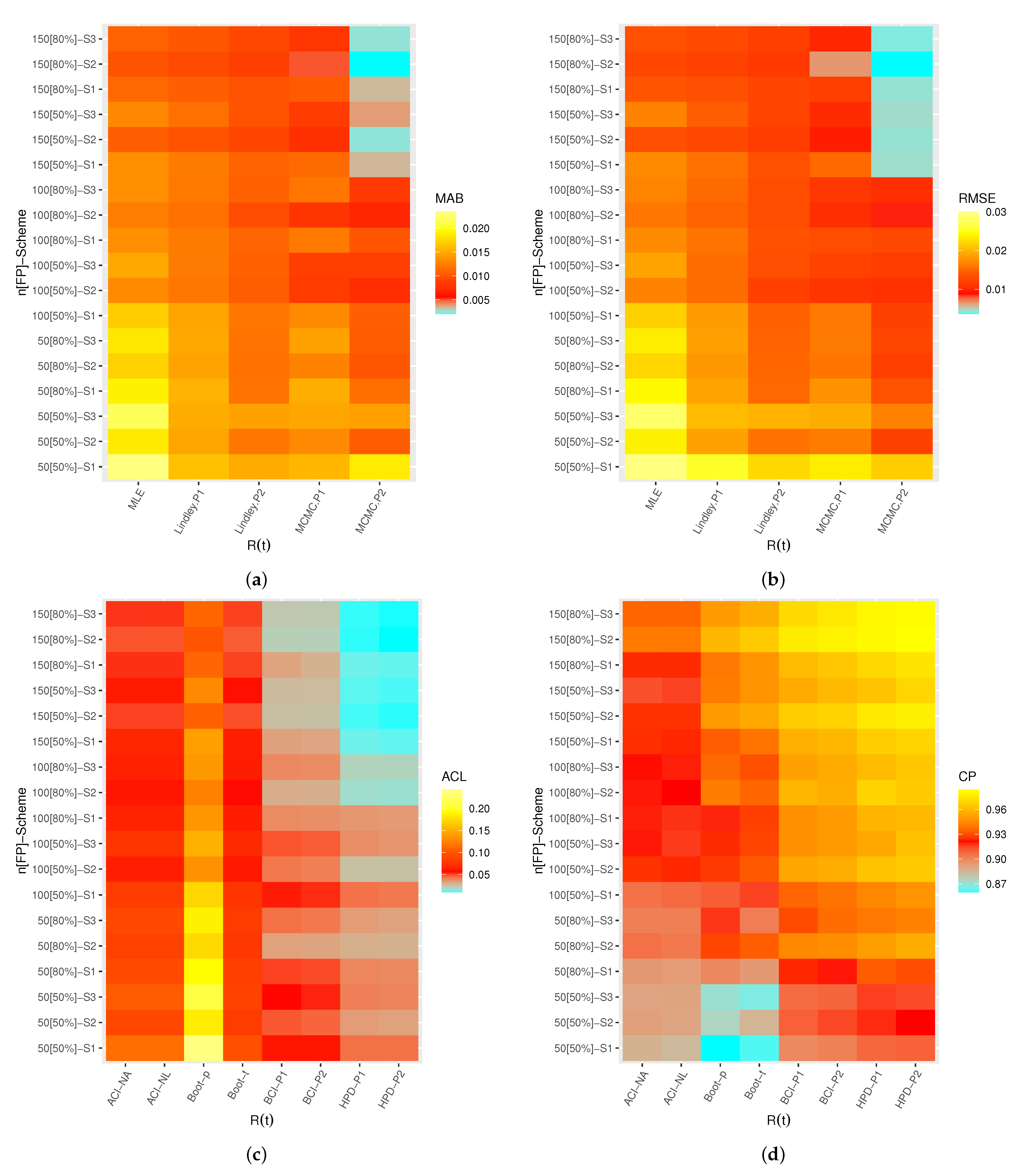
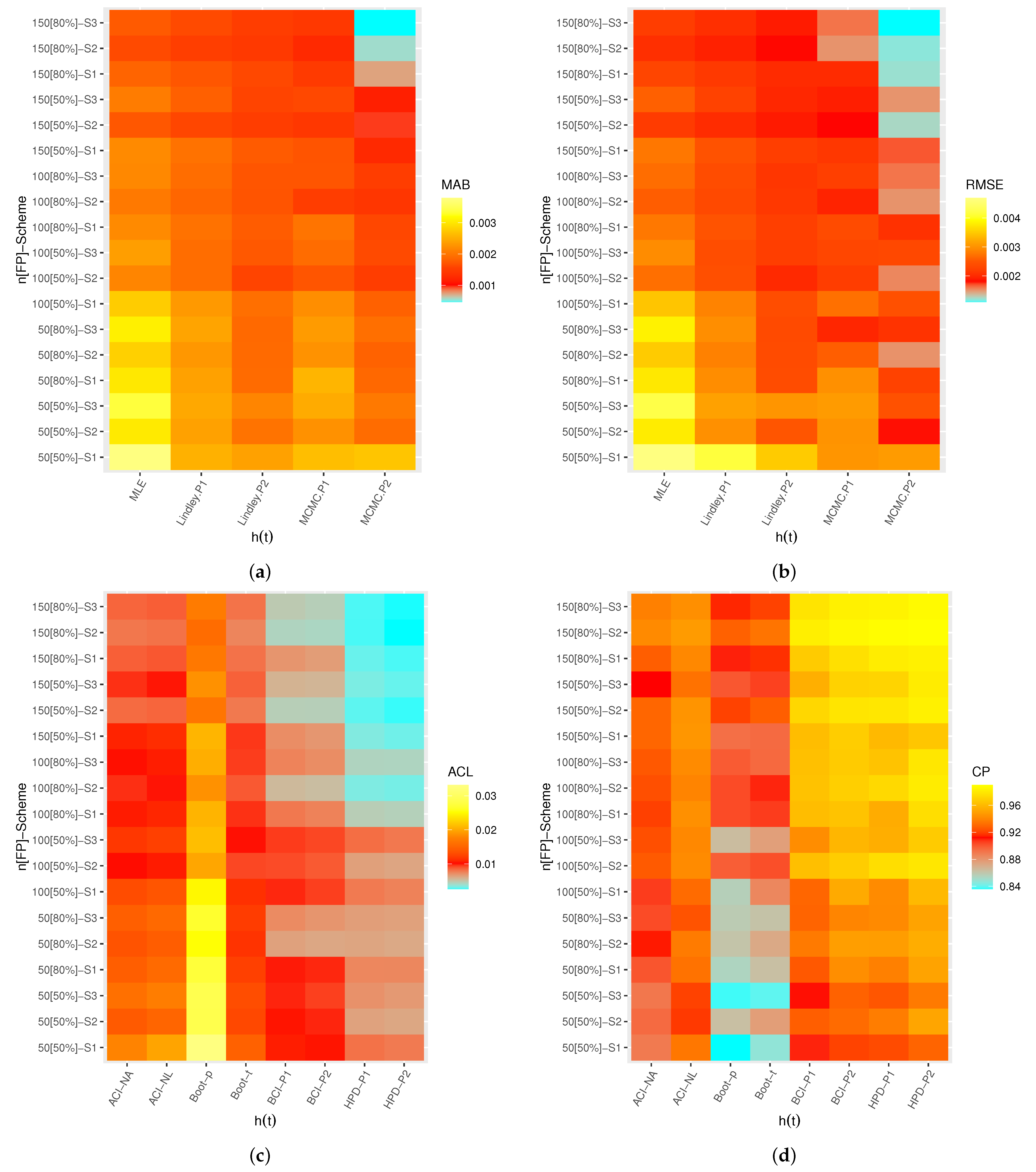
A heatmap is a graphical representation of numerical data used to show relationships between two variables of interest so that individual data points contained in a data set are represented via different colors. Therefore, by software, the heatmap data tool is used to display the simulated results, including: MAB, RMSE, ACL, and CP values of , , , and , see Figure 3, Figure 4, Figure 5 and Figure 6, respectively. Each heatmap displays the proposed estimation methods and the specified test settings on the “” and “” lines, respectively. On the other hand, all simulation results of , , , and are also available in Table 1, Table 2, Table 3 and Table 4.
- Overall, the Bayes MCMC estimates of all unknown parameters perform better than the MLEs in terms of the smallest values of MABs, RMSEs, and ACLs, as well as the highest CP values.
- As n (or m) increases, the MABs, RMSEs, and ACLs tend to decrease (except CPs increase), which infers that the proposed estimates are asymptotically unbiased and consistent. This result is also reached when the total number of progressive items, , decreases.
- Comparing the proposed point estimation methods on the basis of the smallest MABs and RMSEs, it is clear that the performance of MCMC estimates of all unknown parameters is highly recognizable compared to those obtained based on the Lindley approach, and both exhibit reasonably good performance compared to the likelihood method. It is an anticipated result because the calculated MCMC estimates included additional prior information.
- Comparing the proposed interval estimation methods in terms of the smallest ACLs and highest CPs, it is observed that (i) ACI-NA performs better than ACI-NL, (ii) Boot-t performs better than Boot-p, and (iii) the HPD interval performs better than BCI. This conclusion holds for all unknown parameters. It is also clear, in most cases, that the CPs of classical (or Bayes) interval estimates are mostly close to (or below) the specified nominal level.
- In particular, based on the ACL and CP criteria, it is also noted that the HPD interval of all unknown parameters provides the best bounds compared to its competitive intervals.
- Since the variance in P2 is smaller than the variance in P1, consequently, the Bayes estimates (or BCI/HPD intervals) perform better based on P2 than the others.
- Comparing the proposed censoring schemes, both point and interval estimation methods of provide good behavior under (where the survival units are removed in the first stage) compared with other competing schemes. Moreover, both point and interval estimation methods of , , and provide good behavior under (where the survival units are removed in the middle stage) compared to others.
- Lastly, to evaluate the unknown parameter(s) of the WNH lifetime model in the presence of data collected from Type-II progressive censoring, the Bayes MCMC methodology is recommended.
6. Optimum PCTII Fashions
The issue of determining the optimum progressive censoring (removal pattern design ) from a group of all possible plans is a great challenge for any practitioner. In this context, independently, Balakrishnan and Aggarwala [17] and Ng et al. [18] first studied this issue through various setups. The main idea of optimal progressive censoring is, for fixed n and m, that the experimenter chooses the scheme in the sense it provides a significant amount of information of the unknown parameter(s) under study. According to the experimenter’s knowledge about the availability of test items, experimental sources, and test cost, the best censoring plan is selected.
In the literature, for different lifetime models, various works have investigated the problem of optimum censoring; see, for example, Pradhan and Kundu [19], Elshahhat and Nassar [20], Elshahhat and Abu El Azm [7], among others. In Table 5, to select the optimal PCTII plan, several criteria are listed.
From Table 5; regarding criterion 1, the experimenter aims to increase the main diagonal values of the observed Fisher information. Further, regarding criteria 2 and 3, the experimenter aims to reduce the trace and determinant values of the estimated VCov matrix. Under criterion 4, the experimenter aims to minimize the estimated variance in the logarithm of the MLE of th quantile, for .
The optimized censoring should coincide with the largest value of criterion 1 and the smallest value of the other criteria. According to criterion 4, using the delta method, the variance of is given by
where
7. Three Engineering Applications
To show the applicability of the proposed estimation methodologies to real phenomena, we will analyze three different actual data sets. The first data set (say Data A), reported by Mann [21] and re-analyzed by Alotaibi et al. [22], consists of the number of vehicle fatalities for 39 counties in South Carolina in 2012. The second data set (say Data B), given by Wang [23] and discussed earlier by Elshahhat and Abu El Azm [7], represents the times to failure of eighteen electronic devices. The last data set (say Data C), taken from Lawless [24] and Mohammed et al. [25], represents the failure times (in minutes) of fifteen electronic components in an accelerated life test. These data sets are reported in Table 6.
To highlight the flexibility and adaptability of the proposed model, based on different criteria, the WNH distribution is compared with three weighted distributions as competitors, namely: weighted exponential (WE) by Gupta and Kundu [26], weighted Gompertz (WG) by Bakouch et al. [27] and new weighted Lindley (WL) by Asgharzadeh et al. [28] distributions. The respective PDFs of the compared WE, WG, and WL distributions (for and ) are:
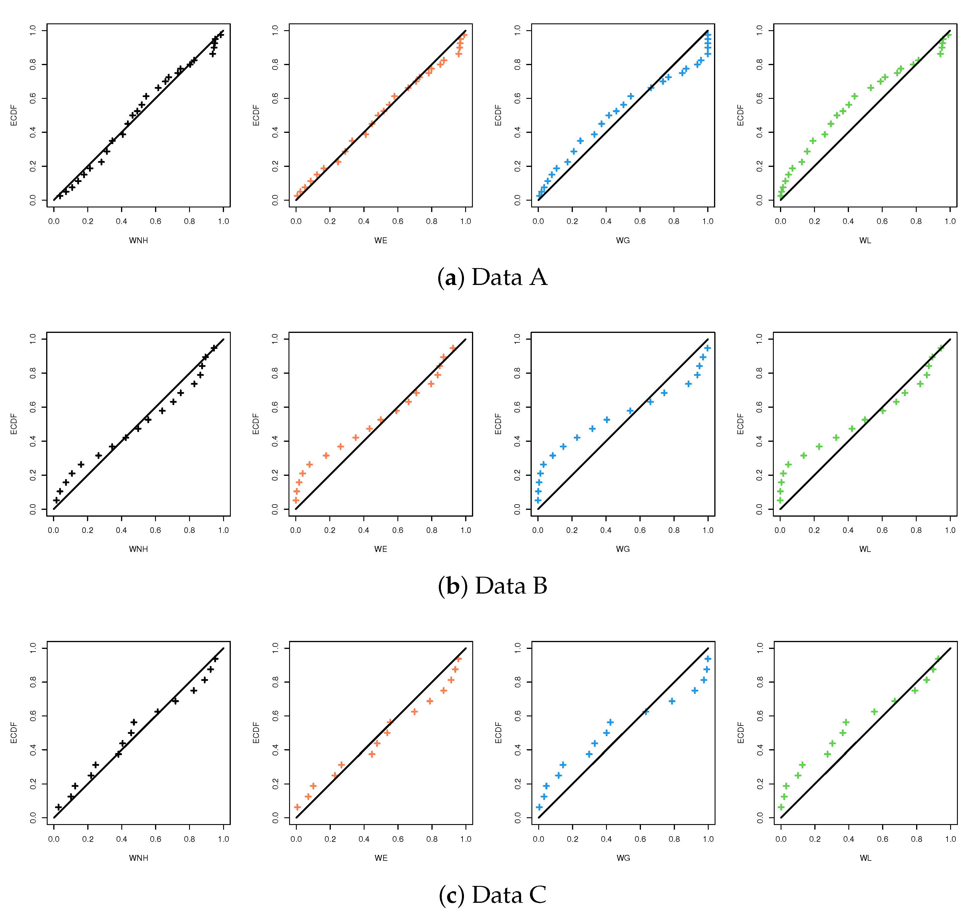
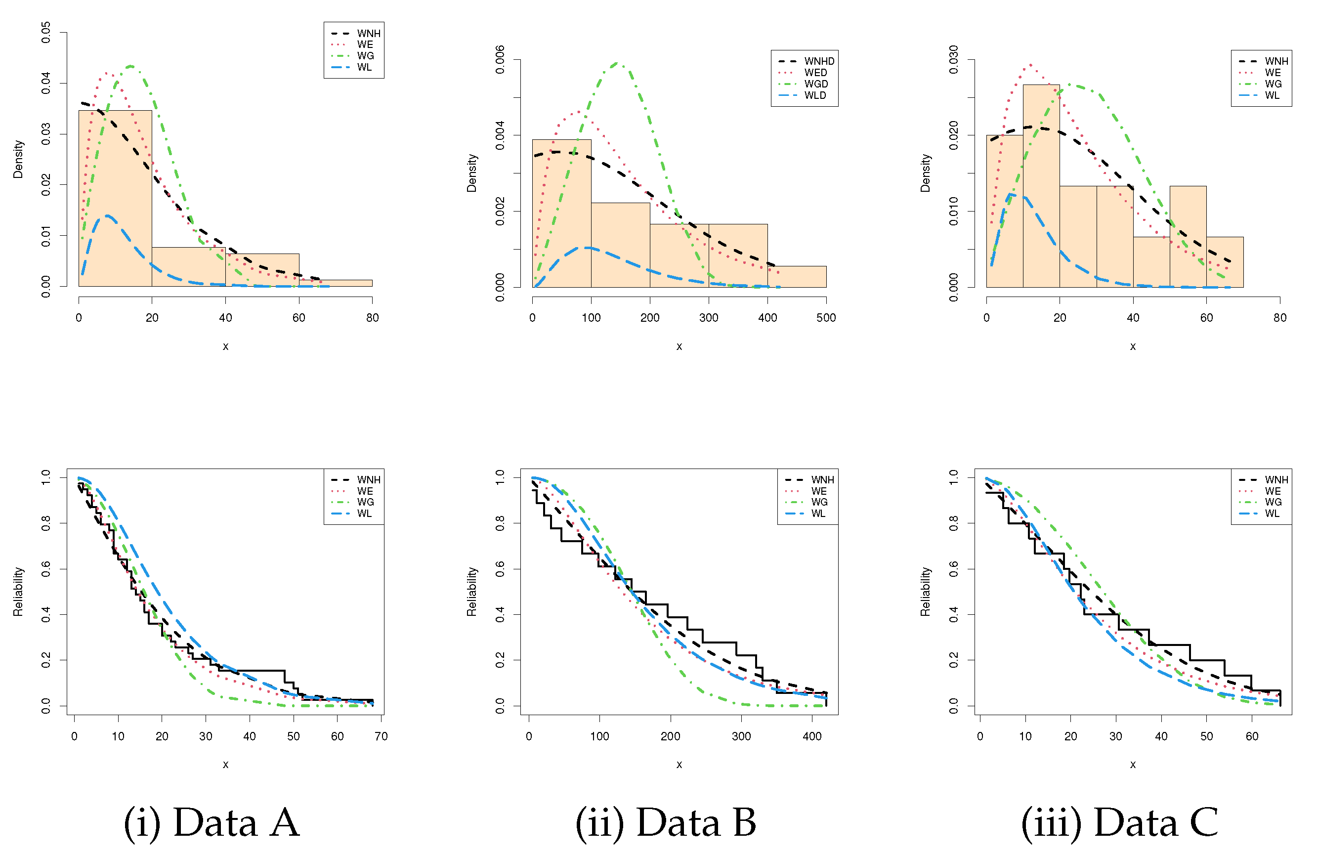
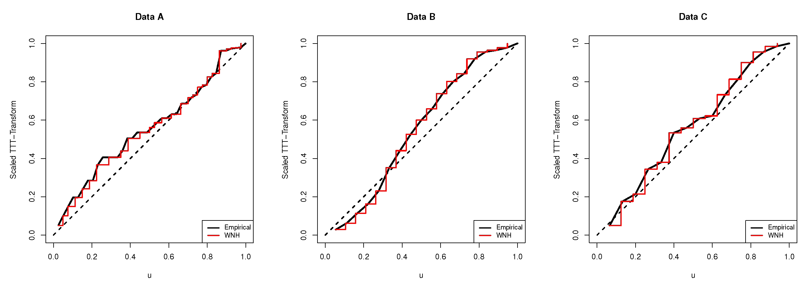
For each data set, the parameter estimates of and with their standard errors (SEs) of each competing model are evaluated by the ML method. Moreover, the estimated values of the negative log-likelihood (NL), Akaike information (AI), consistent Akaike information (CAI), Bayesian information (BI), Hannan–Quinn information (HQI) and the Kolmogorov–Smirnov statistic with its P-value are computed and reported in Table 7. Figure 7 represents the probability-probability (PP) plots of the WNH, WE, WG and WL distributions. It indicates that the plotted points of the fitted WNH distribution based on each data set are quite close to the empirical distribution line. It also confirms the same findings in Table 7. Moreover, Figure 8 displays the estimated PDFs with their histograms as well as the estimated RFs for the compared distributions under the three data sets. It is clear that the fitted WNH density captures the empirical histograms well. To sum up, we concluded that the WNH distribution has a favorable superiority over other weighted distributions because it has the smallest values of the fitting criteria based on the given data sets. For more illustration, for each real data set, the empirical/estimated TTT transform plot of the WNH distribution is provided in Figure 9. It exhibits that the given real data sets have a constant hazard rate function.
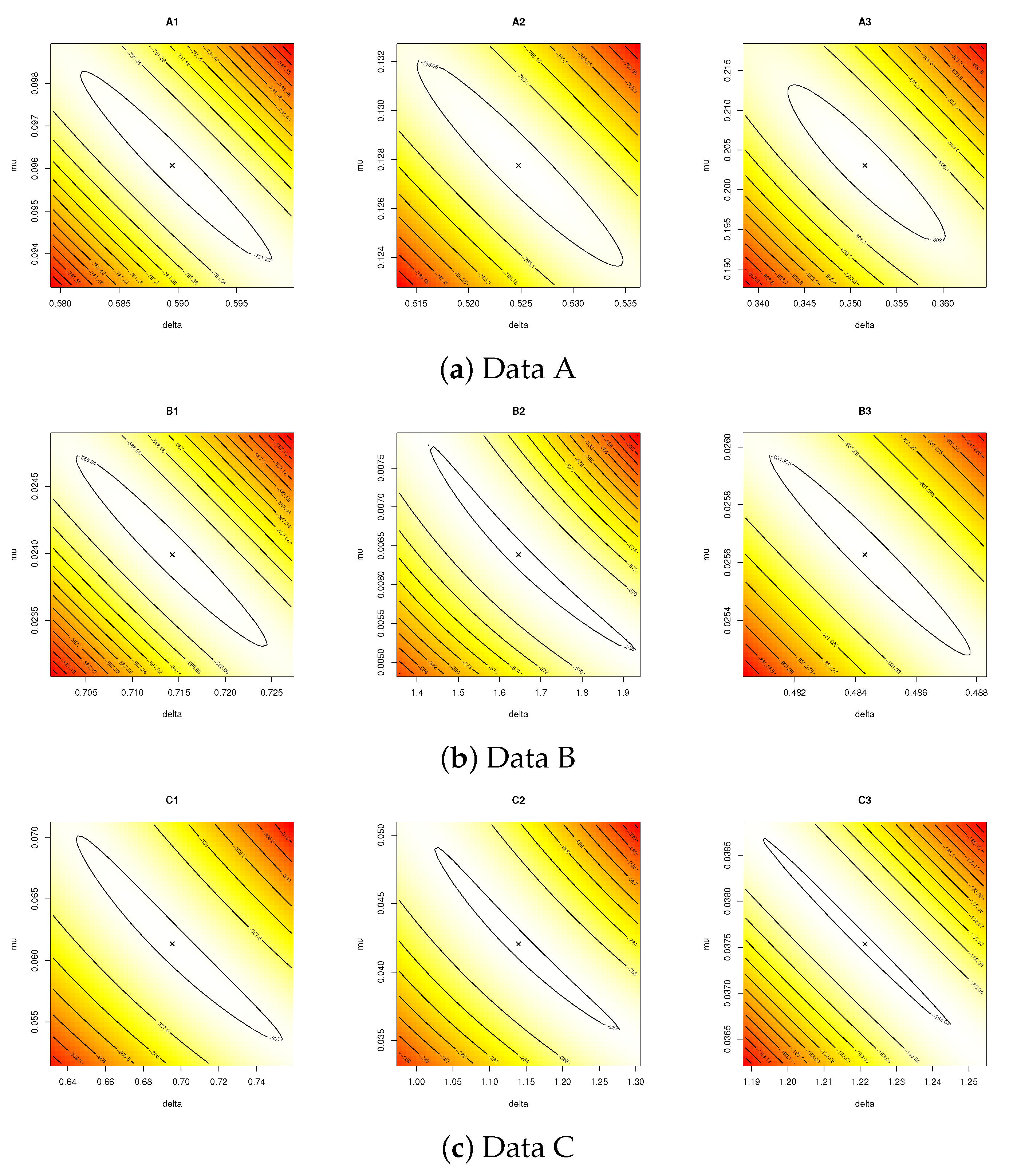
Next, using various choices of m and , three different PCTII samples from each complete real data set are generated and listed in Table 8. For each PCTII sample in Table 8, the theoretical results of , , , and are evaluated numerically via software. The point estimates (including: MLEs, Lindley, and MCMC) with their SEs as well as the 95% interval estimates (including: ACI-NA, ACI-NL, Boot-p, Boot-t, BCI, and HPD) of , , , and (at ) are presented in Table 9 and Table 10, respectively. To examine the uniqueness and existence of the MLEs of and for Ai, Bi, and Ci for samples, the contour plots of the log-likelihood function (7) are shown in Figure 10. It shows that all acquired estimates of and exist and are unique. For obtaining the Bayes MCMC estimates along with their BCI/HPD intervals based on noninformative gamma prior, the M-H algorithm proposed in Section 4.2 is repeated 30,000 times, and the first 5000 draws are thrown out. From Table 9 and Table 10, in terms of minimum standard errors and interval lengths, it can be seen that the MCMC estimates are more precise than the classical estimates. Moreover, the two interval bounds obtained by asymptotic, bootstrap, and credible intervals are close to each other.
In Figure 11, based on samples A1, B1, and C1 (as an example), the simulated estimates with their histograms for the marginal posterior distribution functions of , , , and are plotted with the Gaussian line. It is evident that the MCMC estimates behave appropriately with the normal distribution, where (:) represents the mean sample line. In addition, trace plots using A1, B1, and C1 of the same parameters are displayed in Figure 11 where the sample mean, and BCI/HPD intervals are shown with solid (—), dotted (…), and dashed (- - -) horizontal lines, respectively. It shows that the MCMC iterations based on each generated PCTII sample are mixed well.
Using the generated PCTII samples in Table 8, the optimal progressive censoring plans, with respect to different criteria reported in Table 5, are obtained and reported in Table 11. It is noted, from Table 11, that
- For Data A; the censoring schemes used in samples A1 (with respect to criteria 1 and 3) and A3 (with respect to criteria 2 and 4) are the optimum plans.
- For Data B; the censoring schemes used in samples B1 (with respect to criterion 3), B2 (with respect to criterion 1), and B3 (with respect to criteria 2 and 4) are the optimum plans.
- For Data C; the censoring schemes used in samples C1 (with respect to criteria 2 and 3), C2 (with respect to criterion 1) and C3 (with respect to criterion 4) are the optimum plans.
Table 11 also supports the same results of the proposed censoring plans (S) discussed in the simulation section. Briefly, we concluded that the WNH lifetime model provides a good and adequate explanation of the proposed censoring plan for all given real data sets.
8. Concluding Remarks
This article derives both point and interval estimators of the parameters, reliability, and hazard functions of the new, two-parameter weighted Nadarajah–Haghighi distribution based on Type-II progressive censored sample via the maximum likelihood and Bayesian estimation methods. Further, two parametric bootstrap confidence intervals of the same unknown parameters have been derived. Since the Bayes estimators cannot be written in closed forms, Lindley and MCMC approximations have been investigated. Numerical comparisons have been performed to judge the behavior of the proposed estimators, and they showed that the Bayes estimates using the Metropolis–Hastings algorithm behave well compared to Lindley’s procedure, and both behave much better than the frequentist estimates. Three real data sets taken from several areas, namely: insurance, reliability, and accelerated life testing, have been analyzed to show the usefulness of the proposed model in real practice. All theoretical results have been evaluated utilizing two useful packages in software, namely: ‘’ and ‘’ packages. As a result, the Bayes MCMC paradigm is recommended to estimate the model parameters and/or the reliability characteristic of the weighted Nadarajah–Haghighi model in the presence of a sample obtained from Type-II progressive censoring. As a future work, one can extend the results and methodologies discussed here to accelerate life tests or other censoring plans. We also hope that the proposed methodologies will be beneficial to researchers and reliability practitioners.
Author Contributions
Methodology, A.E. and H.S.M.; Funding acquisition, H.S.M.; Software, A.E.; Supervision A.E.; Writing—original draft, H.S.M.; Writing—review and editing A.E. All authors have read and agreed to the published version of the manuscript.
Funding
This research was funded by Princess Nourah bint Abdulrahman University Researchers Supporting Project number (PNURSP2023R175), Princess Nourah bint Abdulrahman University, Riyadh, Saudi Arabia.
Data Availability Statement
The authors confirm that the data supporting the findings of this study are available within the article.
Acknowledgments
The authors would also like to express their gratitude to the Editor-in-Chief and anonymous referees for their constructive comments and suggestions, which significantly improved the paper. Princess Nourah bint Abdulrahman University Researchers Supporting Project number (PNURSP2023R175), Princess Nourah bint Abdulrahman University, Riyadh, Saudi Arabia.
Conflicts of Interest
The authors declare no conflict of interest.
Appendix A
Fisher elements from (7) with respect to and are
and
where is the second-partial derivative with respect to for as
, ,
and
Appendix B
Lindley’s elements from (7) with respect to and are
where is the third-partial derivative with respect to for as
and .
Appendix C
References
- Nadarajah, S.; Haghighi, F. An extension of the exponential distribution. Statistics 2011, 45, 543–558. [Google Scholar] [CrossRef]
- Khan, M.N.; Saboor, A.; Cordeiro, G.M.; Nazir, M.; Pescim, R.R. A weighted Nadarajah and Haghighi distribution. Upb Sci. Bull. Ser. Appl. Math. Phys. 2018, 80, 133–140. [Google Scholar]
- Mohie El-Din, M.M.; Abu-Youssef, S.E.; Ali, N.S.; Abd El-Raheem, A.M. Classical and Bayesian inference on progressive-stress accelerated life testing for the extension of the exponential distribution under progressive type-II censoring. Qual. Reliab. Eng. Int. 2017, 33, 2483–2496. [Google Scholar] [CrossRef]
- Ashour, S.K.; El-Sheikh, A.A.; Elshahhat, A. Inferences and optimal censoring schemes for progressively first-failure censored Nadarajah-Haghighi distribution. Sankhya A 2020, 84, 885–923. [Google Scholar] [CrossRef]
- Wu, M.; Gui, W. Estimation and prediction for Nadarajah-Haghighi distribution under progressive type-II censoring. Symmetry 2021, 13, 999. [Google Scholar] [CrossRef]
- Elshahhat, A.; Alotaibi, R.; Nassar, M. Inferences for Nadarajah–Haghighi Parameters via Type-II Adaptive Progressive Hybrid Censoring with Applications. Mathematics 2022, 10, 3775. [Google Scholar] [CrossRef]
- Elshahhat, A.; Abu El Azm, W.S. Statistical reliability analysis of electronic devices using generalized progressively hybrid censoring plan. Qual. Reliab. Eng. Int. 2022, 38, 1112–1130. [Google Scholar] [CrossRef]
- Dey, S.; Wang, L.; Nassar, M. Inference on Nadarajah–Haghighi distribution with constant stress partially accelerated life tests under progressive type-II censoring. J. Appl. Stat. 2022, 49, 2891–2912. [Google Scholar] [CrossRef]
- Almarashi, A.M.; Algarni, A.; Okasha, H.; Nassar, M. On reliability estimation of Nadarajah–Haghighi distribution under adaptive type-I progressive hybrid censoring scheme. Qual. Reliab. Eng. Int. 2022, 38, 817–833. [Google Scholar] [CrossRef]
- Henningsen, A.; Toomet, O. ‘maxLik’: A package for maximum likelihood estimation in R. Comput. Stat. 2011, 26, 443–458. [Google Scholar] [CrossRef]
- Greene, W.H. Econometric Analysis, 7th ed.; Pearson Prentice-Hall: Upper Saddle River, NJ, USA, 2012. [Google Scholar]
- Meeker, W.Q.; Escobar, L.A. Statistical Methods for Reliability Data; John Wiley and Sons: New York, NY, USA, 1998. [Google Scholar]
- Kundu, D. Bayesian inference and life testing plan for the Weibull distribution in presence of progressive censoring. Technometrics 2008, 50, 144–154. [Google Scholar] [CrossRef]
- Lindley, D.V. Approximate Bayesian methods. Trab Estad. 1980, 31, 223–245. [Google Scholar] [CrossRef]
- Gelman, A.; Carlin, J.B.; Stern, H.S.; Dunson, D.B.; Vehtari, A.; Rubin, D.B. Bayesian Data Analysis, 2nd ed.Chapman and Hall/CRC: Boca Raton, FL, USA, 2004. [Google Scholar]
- Plummer, M.; Best, N.; Cowles, K.; Vines, K. ‘coda’: Convergence diagnosis and output analysis for MCMC. R News 2006, 6, 7–11. [Google Scholar]
- Balakrishnan, N.; Aggarwala, R. Progressive Censoring: Theory, Methods, and Applications; Springer Science and Business Media, Birkhäuser: Boston, MA, USA, 2000. [Google Scholar]
- Ng, H.K.T.; Chan, P.S.; Balakrishnan, N. Optimal progressive censoring plans for the Weibull distribution. Technometrics 2004, 46, 470–481. [Google Scholar] [CrossRef]
- Pradhan, B.; Kundu, D. Inference and optimal censoring schemes for progressively censored Birnbaum-Saunders distribution. J. Stat. Plan. Inference 2013, 143, 1098–1108. [Google Scholar] [CrossRef]
- Elshahhat, A.; Nassar, M. Bayesian survival analysis for adaptive Type-II progressive hybrid censored Hjorth data. Comput. Stat. 2021, 36, 1965–1990. [Google Scholar] [CrossRef]
- Mann, S.P. Introductory Statistics; Wiley Publisher: Hoboken, NJ, USA, 2016. [Google Scholar]
- Alotaibi, R.; Rezk, H.; Elshahhat, A. Computational Analysis for Fréchet Parameters of Life from Generalized Type-II Progressive Hybrid Censored Data with Applications in Physics and Engineering. Symmetry 2023, 15, 348. [Google Scholar] [CrossRef]
- Wang, F.K. A new model with bathtub-shaped failure rate using an additive Burr XII distribution. Reliab. Eng. Syst. Saf. 2000, 70, 305–312. [Google Scholar] [CrossRef]
- Lawless, J.F. Statistical Models and Methods for Lifetime Data, 2nd ed.Wiley Publisher: Hoboken, NJ, USA, 2003. [Google Scholar]
- Mohammed, H.S.; Nassar, M.; Alotaibi, R.; Elshahhat, A. Analysis of Adaptive Progressive Type-II Hybrid Censored Dagum Data with Applications. Symmetry 2022, 14, 2146. [Google Scholar] [CrossRef]
- Gupta, R.D.; Kundu, D. A new class of weighted exponential distributions. Statistics 2009, 43, 621–634. [Google Scholar] [CrossRef]
- Bakouch, H.S.; El-Bar, A.; Ahmed, M.T. A new weighted Gompertz distribution with applications to reliability data. Appl. Math. 2017, 62, 269–296. [Google Scholar] [CrossRef]
- Asgharzadeh, A.; Bakouch, H.S.; Nadarajah, S.; Sharafi, F. A new weighted Lindley distribution with application. Braz. J. Probab. Stat. 2016, 30, 1–27. [Google Scholar] [CrossRef]
Figure 1.
Density (left) and hazard rate (right) shapes of the WNH distribution.

Figure 2.
Conditional PDFs of and .

Figure 3.
Heatmaps for the simulation results of MAB (a), RMSE (b), ACL (c), and CP (d) for .

Figure 4.
Heatmaps for the simulation results of MAB (a), RMSE (b), ACL (c), and CP (d) for .

Figure 5.
Heatmaps for the simulation results of MAB (a), RMSE (b), ACL (c), and CP (d) for .

Figure 6.
Heatmaps for the simulation results of MAB (a), RMSE (b), ACL (c), and CP (d) for .

Figure 7.
The PP plots of the WNH distribution and its competitive models under three real data sets.
Figure 7.
The PP plots of the WNH distribution and its competitive models under three real data sets.

Figure 8.
The estimated PDFs (left) and estimated RFs (right) of the competing models under the three real data sets.
Figure 8.
The estimated PDFs (left) and estimated RFs (right) of the competing models under the three real data sets.

Figure 9.
TTT-Transform plots of the WNH distribution under the three real data sets.

Figure 10.
Contour plots of the log-likelihood function of and from the three data sets.

Figure 11.
Histograms (top) and Trace (bottom) plots of , , , and from the real data sets.


Table 1.
The point estimation results of and .
| Par. | Scheme | MLE | Lindley | MCMC | ||||||||
|---|---|---|---|---|---|---|---|---|---|---|---|---|
| Prior → | 1 | 2 | 1 | 2 | ||||||||
| MAB | RMSE | MAB | RMSE | MAB | RMSE | MAB | RMSE | MAB | RMSE | |||
| (50,25) | S1 | 0.0570 | 0.0832 | 0.0416 | 0.0571 | 0.0309 | 0.0489 | 0.0333 | 0.0561 | 0.0255 | 0.0417 | |
| S2 | 0.0640 | 0.1025 | 0.0491 | 0.0894 | 0.0401 | 0.0745 | 0.0357 | 0.0583 | 0.0261 | 0.0442 | ||
| S3 | 0.1107 | 0.5980 | 0.0766 | 0.0992 | 0.0630 | 0.0841 | 0.0456 | 0.0644 | 0.0395 | 0.0630 | ||
| (50,40) | S1 | 0.0423 | 0.0575 | 0.0355 | 0.0481 | 0.0284 | 0.0409 | 0.0263 | 0.0432 | 0.0192 | 0.0380 | |
| S2 | 0.0426 | 0.0592 | 0.0360 | 0.0492 | 0.0290 | 0.0411 | 0.0265 | 0.0473 | 0.0213 | 0.0387 | ||
| S3 | 0.0478 | 0.0687 | 0.0399 | 0.0559 | 0.0303 | 0.0500 | 0.0333 | 0.0527 | 0.0293 | 0.0412 | ||
| (100,50) | S1 | 0.0367 | 0.0493 | 0.0323 | 0.0433 | 0.0274 | 0.0365 | 0.0272 | 0.0388 | 0.0209 | 0.0354 | |
| S2 | 0.0381 | 0.0525 | 0.0342 | 0.0467 | 0.0303 | 0.0406 | 0.0307 | 0.0409 | 0.0216 | 0.0397 | ||
| S3 | 0.0518 | 0.0740 | 0.0460 | 0.0631 | 0.0341 | 0.0437 | 0.0399 | 0.0455 | 0.0258 | 0.0427 | ||
| (100,80) | S1 | 0.0281 | 0.0364 | 0.0259 | 0.0335 | 0.0235 | 0.0304 | 0.0228 | 0.0321 | 0.0189 | 0.0300 | |
| S2 | 0.0276 | 0.0357 | 0.0255 | 0.0384 | 0.0234 | 0.0301 | 0.0286 | 0.0360 | 0.0207 | 0.0309 | ||
| S3 | 0.0320 | 0.0419 | 0.0295 | 0.0418 | 0.0264 | 0.0345 | 0.0317 | 0.0414 | 0.0212 | 0.0327 | ||
| (150,75) | S1 | 0.0276 | 0.0362 | 0.0253 | 0.0369 | 0.0229 | 0.0300 | 0.0218 | 0.0337 | 0.0129 | 0.0302 | |
| S2 | 0.0299 | 0.0392 | 0.0279 | 0.0403 | 0.0259 | 0.0337 | 0.0226 | 0.0364 | 0.0137 | 0.0314 | ||
| S3 | 0.0405 | 0.0543 | 0.0378 | 0.0507 | 0.0322 | 0.0421 | 0.0291 | 0.0423 | 0.0149 | 0.0366 | ||
| (150,120) | S1 | 0.0221 | 0.0282 | 0.0209 | 0.0267 | 0.0197 | 0.0252 | 0.0200 | 0.0260 | 0.0118 | 0.0242 | |
| S2 | 0.0224 | 0.0292 | 0.0213 | 0.0277 | 0.0201 | 0.0262 | 0.0201 | 0.0268 | 0.0133 | 0.0244 | ||
| S3 | 0.0240 | 0.0313 | 0.0228 | 0.0298 | 0.0213 | 0.0277 | 0.0208 | 0.0285 | 0.0137 | 0.0267 | ||
| (50,25) | S1 | 0.0628 | 0.0950 | 0.0586 | 0.0965 | 0.0531 | 0.0931 | 0.0410 | 0.0605 | 0.0384 | 0.0542 | |
| S2 | 0.0511 | 0.0741 | 0.0477 | 0.0787 | 0.0393 | 0.0618 | 0.0255 | 0.0571 | 0.0328 | 0.0513 | ||
| S3 | 0.0716 | 0.1710 | 0.2377 | 0.1840 | 0.1335 | 0.1471 | 0.0561 | 0.0708 | 0.0555 | 0.0641 | ||
| (50,40) | S1 | 0.0470 | 0.0680 | 0.0440 | 0.0769 | 0.0354 | 0.0595 | 0.0362 | 0.0545 | 0.0251 | 0.0484 | |
| S2 | 0.0449 | 0.0655 | 0.0433 | 0.0686 | 0.0352 | 0.0597 | 0.0253 | 0.0520 | 0.0204 | 0.0434 | ||
| S3 | 0.0507 | 0.0737 | 0.0474 | 0.0805 | 0.0372 | 0.0607 | 0.0403 | 0.0627 | 0.0308 | 0.0542 | ||
| (100,50) | S1 | 0.0434 | 0.0618 | 0.0415 | 0.0525 | 0.0305 | 0.0387 | 0.0347 | 0.0507 | 0.0287 | 0.0336 | |
| S2 | 0.0350 | 0.0468 | 0.0354 | 0.0473 | 0.0290 | 0.0353 | 0.0246 | 0.0445 | 0.0283 | 0.0317 | ||
| S3 | 0.0429 | 0.0591 | 0.0396 | 0.0554 | 0.0332 | 0.0472 | 0.0391 | 0.0513 | 0.0302 | 0.0405 | ||
| (100,80) | S1 | 0.0340 | 0.0471 | 0.0337 | 0.0459 | 0.0293 | 0.0375 | 0.0334 | 0.0430 | 0.0226 | 0.0326 | |
| S2 | 0.0316 | 0.0428 | 0.0320 | 0.0433 | 0.0285 | 0.0349 | 0.0261 | 0.0402 | 0.0218 | 0.0305 | ||
| S3 | 0.0354 | 0.0475 | 0.0351 | 0.0468 | 0.0302 | 0.0382 | 0.0340 | 0.0443 | 0.0283 | 0.0375 | ||
| (150,75) | S1 | 0.0336 | 0.0458 | 0.0337 | 0.0456 | 0.0291 | 0.0373 | 0.0257 | 0.0329 | 0.0207 | 0.0266 | |
| S2 | 0.0279 | 0.0367 | 0.0282 | 0.0375 | 0.0258 | 0.0335 | 0.0215 | 0.0324 | 0.0196 | 0.0249 | ||
| S3 | 0.0376 | 0.0519 | 0.0361 | 0.0487 | 0.0289 | 0.0375 | 0.0339 | 0.0331 | 0.0268 | 0.0286 | ||
| (150,120) | S1 | 0.0275 | 0.0360 | 0.0278 | 0.0369 | 0.0257 | 0.0334 | 0.0234 | 0.0295 | 0.0129 | 0.0232 | |
| S2 | 0.0254 | 0.0331 | 0.0257 | 0.0341 | 0.0240 | 0.0313 | 0.0205 | 0.0236 | 0.0126 | 0.0215 | ||
| S3 | 0.0276 | 0.0368 | 0.0277 | 0.0374 | 0.0254 | 0.0334 | 0.0244 | 0.0318 | 0.0139 | 0.0261 | ||
Table 2.
The point estimation results of and .
| Par. | Scheme | MLE | Lindley | MCMC | ||||||||
|---|---|---|---|---|---|---|---|---|---|---|---|---|
| Prior → | 1 | 2 | 1 | 2 | ||||||||
| MAB | RMSE | MAB | RMSE | MAB | RMSE | MAB | RMSE | MAB | RMSE | |||
| (50,25) | S1 | 0.0235 | 0.0301 | 0.0164 | 0.0255 | 0.0152 | 0.0224 | 0.0159 | 0.0237 | 0.0188 | 0.0217 | |
| S2 | 0.0188 | 0.0240 | 0.0148 | 0.0189 | 0.0122 | 0.0158 | 0.0132 | 0.0164 | 0.0106 | 0.0122 | ||
| S3 | 0.0219 | 0.0287 | 0.0152 | 0.0206 | 0.0147 | 0.0201 | 0.0149 | 0.0196 | 0.0145 | 0.0167 | ||
| (50,40) | S1 | 0.0192 | 0.0245 | 0.0156 | 0.0190 | 0.0120 | 0.0152 | 0.0153 | 0.0178 | 0.0117 | 0.0139 | |
| S2 | 0.0173 | 0.0222 | 0.0147 | 0.0183 | 0.0118 | 0.0151 | 0.0129 | 0.0160 | 0.0102 | 0.0120 | ||
| S3 | 0.0186 | 0.0236 | 0.0150 | 0.0188 | 0.0119 | 0.0149 | 0.0146 | 0.0163 | 0.0106 | 0.0126 | ||
| (100,50) | S1 | 0.0171 | 0.0218 | 0.0148 | 0.0184 | 0.0121 | 0.0148 | 0.0133 | 0.0162 | 0.0107 | 0.0121 | |
| S2 | 0.0133 | 0.0169 | 0.0122 | 0.0154 | 0.0107 | 0.0121 | 0.0087 | 0.0111 | 0.0075 | 0.0109 | ||
| S3 | 0.0150 | 0.0190 | 0.0124 | 0.0155 | 0.0108 | 0.0136 | 0.0090 | 0.0122 | 0.0090 | 0.0117 | ||
| (100,80) | S1 | 0.0135 | 0.0174 | 0.0124 | 0.0159 | 0.0111 | 0.0138 | 0.0122 | 0.0133 | 0.0102 | 0.0128 | |
| S2 | 0.0126 | 0.0161 | 0.0117 | 0.0149 | 0.0098 | 0.0134 | 0.0082 | 0.0107 | 0.0071 | 0.0088 | ||
| S3 | 0.0136 | 0.0170 | 0.0123 | 0.0154 | 0.0108 | 0.0133 | 0.0121 | 0.0113 | 0.0087 | 0.0106 | ||
| (150,75) | S1 | 0.0135 | 0.0173 | 0.0124 | 0.0158 | 0.0110 | 0.0137 | 0.0113 | 0.0153 | 0.0035 | 0.0047 | |
| S2 | 0.0107 | 0.0135 | 0.0101 | 0.0128 | 0.0094 | 0.0118 | 0.0077 | 0.0097 | 0.0026 | 0.0046 | ||
| S3 | 0.0132 | 0.0168 | 0.0117 | 0.0147 | 0.0101 | 0.0125 | 0.0087 | 0.0105 | 0.0040 | 0.0047 | ||
| (150,120) | S1 | 0.0112 | 0.0142 | 0.0107 | 0.0135 | 0.0100 | 0.0125 | 0.0105 | 0.0118 | 0.0035 | 0.0045 | |
| S2 | 0.0101 | 0.0127 | 0.0097 | 0.0122 | 0.0091 | 0.0114 | 0.0051 | 0.0067 | 0.0021 | 0.0037 | ||
| S3 | 0.0109 | 0.0137 | 0.0103 | 0.0130 | 0.0095 | 0.0120 | 0.0083 | 0.0102 | 0.0026 | 0.0043 | ||
| (50,25) | S1 | 0.0038 | 0.0047 | 0.0026 | 0.0042 | 0.0024 | 0.0035 | 0.0027 | 0.0031 | 0.0027 | 0.0031 | |
| S2 | 0.0031 | 0.0038 | 0.0024 | 0.0030 | 0.0020 | 0.0025 | 0.0023 | 0.0030 | 0.0019 | 0.0018 | ||
| S3 | 0.0034 | 0.0042 | 0.0025 | 0.0032 | 0.0022 | 0.0031 | 0.0025 | 0.0031 | 0.0021 | 0.0025 | ||
| (50,40) | S1 | 0.0030 | 0.0038 | 0.0024 | 0.0030 | 0.0019 | 0.0024 | 0.0026 | 0.0030 | 0.0019 | 0.0023 | |
| S2 | 0.0028 | 0.0035 | 0.0023 | 0.0029 | 0.0019 | 0.0024 | 0.0023 | 0.0026 | 0.0018 | 0.0015 | ||
| S3 | 0.0031 | 0.0039 | 0.0024 | 0.0030 | 0.0019 | 0.0024 | 0.0024 | 0.0020 | 0.0020 | 0.0021 | ||
| (100,50) | S1 | 0.0028 | 0.0035 | 0.0023 | 0.0029 | 0.0020 | 0.0024 | 0.0022 | 0.0027 | 0.0018 | 0.0025 | |
| S2 | 0.0022 | 0.0027 | 0.0019 | 0.0024 | 0.0016 | 0.0020 | 0.0017 | 0.0022 | 0.0015 | 0.0016 | ||
| S3 | 0.0024 | 0.0030 | 0.0019 | 0.0024 | 0.0018 | 0.0022 | 0.0019 | 0.0023 | 0.0016 | 0.0023 | ||
| (100,80) | S1 | 0.0022 | 0.0028 | 0.0020 | 0.0025 | 0.0018 | 0.0022 | 0.0020 | 0.0024 | 0.0016 | 0.0021 | |
| S2 | 0.0021 | 0.0026 | 0.0019 | 0.0024 | 0.0017 | 0.0021 | 0.0015 | 0.0020 | 0.0014 | 0.0015 | ||
| S3 | 0.0022 | 0.0027 | 0.0019 | 0.0024 | 0.0017 | 0.0021 | 0.0017 | 0.0022 | 0.0015 | 0.0016 | ||
| (150,75) | S1 | 0.0022 | 0.0028 | 0.0020 | 0.0025 | 0.0018 | 0.0022 | 0.0017 | 0.0021 | 0.0013 | 0.0017 | |
| S2 | 0.0017 | 0.0022 | 0.0016 | 0.0020 | 0.0015 | 0.0019 | 0.0014 | 0.0018 | 0.0010 | 0.0013 | ||
| S3 | 0.0021 | 0.0026 | 0.0018 | 0.0023 | 0.0016 | 0.0020 | 0.0016 | 0.0019 | 0.0012 | 0.0015 | ||
| (150,120) | S1 | 0.0019 | 0.0023 | 0.0017 | 0.0022 | 0.0016 | 0.0020 | 0.0015 | 0.0020 | 0.0008 | 0.0012 | |
| S2 | 0.0016 | 0.0021 | 0.0015 | 0.0019 | 0.0015 | 0.0018 | 0.0013 | 0.0015 | 0.0006 | 0.0012 | ||
| S3 | 0.0018 | 0.0022 | 0.0016 | 0.0021 | 0.0015 | 0.0019 | 0.0015 | 0.0016 | 0.0005 | 0.0011 | ||
Table 3.
The interval estimation results of and .
| Scheme | ACI-NA | Boot-p | BCI-P1 | BCI-P2 | ACI-NA | Boot-p | BCI-P1 | BCI-P2 | |||||||||
|---|---|---|---|---|---|---|---|---|---|---|---|---|---|---|---|---|---|
| ACI-NL | Boot-t | HPD-P1 | HPD-P2 | ACI-NL | Boot-t | HPD-P1 | HPD-P2 | ||||||||||
| Par.→ | |||||||||||||||||
| ACL | CP | ACL | CP | ACL | CP | ACL | CP | ACL | CP | ACL | CP | ACL | CP | ACL | CP | ||
| (50,25) | S1 | 0.269 | 0.967 | 1.242 | 0.936 | 0.165 | 0.964 | 0.119 | 0.978 | 0.338 | 0.848 | 1.411 | 0.915 | 0.173 | 0.919 | 0.162 | 0.919 |
| 0.278 | 0.949 | 0.494 | 0.939 | 0.155 | 0.987 | 0.108 | 0.980 | 0.481 | 0.947 | 0.408 | 0.920 | 0.158 | 0.954 | 0.146 | 0.968 | ||
| S2 | 0.292 | 0.972 | 1.583 | 0.908 | 0.175 | 0.952 | 0.135 | 0.975 | 0.260 | 0.845 | 0.806 | 0.919 | 0.170 | 0.920 | 0.137 | 0.919 | |
| 0.304 | 0.940 | 0.624 | 0.961 | 0.164 | 0.982 | 0.125 | 0.974 | 0.333 | 0.928 | 0.281 | 0.914 | 0.160 | 0.960 | 0.131 | 0.962 | ||
| S3 | 0.756 | 0.965 | 1.854 | 0.899 | 0.188 | 0.954 | 0.146 | 0.967 | 0.376 | 0.833 | 1.432 | 0.913 | 0.251 | 0.910 | 0.163 | 0.916 | |
| 0.786 | 0.978 | 0.956 | 0.984 | 0.177 | 0.990 | 0.133 | 0.989 | 0.566 | 0.956 | 0.407 | 0.916 | 0.224 | 0.946 | 0.147 | 0.956 | ||
| (50,40) | S1 | 0.203 | 0.975 | 0.616 | 0.928 | 0.149 | 0.964 | 0.111 | 0.982 | 0.243 | 0.855 | 0.916 | 0.918 | 0.169 | 0.925 | 0.129 | 0.925 |
| 0.206 | 0.953 | 0.263 | 0.970 | 0.136 | 0.988 | 0.104 | 0.983 | 0.303 | 0.944 | 0.300 | 0.927 | 0.158 | 0.965 | 0.117 | 0.973 | ||
| S2 | 0.207 | 0.973 | 0.649 | 0.920 | 0.160 | 0.961 | 0.117 | 0.978 | 0.234 | 0.873 | 0.770 | 0.920 | 0.145 | 0.935 | 0.114 | 0.940 | |
| 0.211 | 0.955 | 0.281 | 0.972 | 0.149 | 0.989 | 0.110 | 0.981 | 0.286 | 0.946 | 0.269 | 0.924 | 0.132 | 0.975 | 0.104 | 0.979 | ||
| S3 | 0.230 | 0.970 | 0.825 | 0.940 | 0.172 | 0.967 | 0.168 | 0.981 | 0.265 | 0.860 | 0.956 | 0.915 | 0.178 | 0.926 | 0.135 | 0.929 | |
| 0.236 | 0.953 | 0.347 | 0.971 | 0.161 | 0.989 | 0.152 | 0.983 | 0.335 | 0.940 | 0.309 | 0.919 | 0.168 | 0.969 | 0.122 | 0.973 | ||
| (100,50) | S1 | 0.174 | 0.957 | 0.443 | 0.926 | 0.096 | 0.953 | 0.091 | 0.967 | 0.218 | 0.878 | 0.677 | 0.929 | 0.154 | 0.942 | 0.136 | 0.946 |
| 0.176 | 0.947 | 0.200 | 0.966 | 0.086 | 0.985 | 0.086 | 0.979 | 0.258 | 0.938 | 0.245 | 0.931 | 0.140 | 0.975 | 0.132 | 0.975 | ||
| S2 | 0.181 | 0.961 | 0.482 | 0.931 | 0.163 | 0.958 | 0.114 | 0.972 | 0.176 | 0.894 | 0.519 | 0.930 | 0.133 | 0.951 | 0.110 | 0.959 | |
| 0.183 | 0.943 | 0.219 | 0.963 | 0.147 | 0.983 | 0.107 | 0.974 | 0.198 | 0.945 | 0.202 | 0.938 | 0.124 | 0.982 | 0.104 | 0.987 | ||
| S3 | 0.258 | 0.966 | 1.034 | 0.974 | 0.317 | 0.982 | 0.165 | 0.987 | 0.227 | 0.891 | 0.757 | 0.927 | 0.166 | 0.948 | 0.157 | 0.956 | |
| 0.266 | 0.969 | 0.420 | 0.978 | 0.300 | 0.987 | 0.151 | 0.996 | 0.275 | 0.957 | 0.266 | 0.930 | 0.152 | 0.974 | 0.146 | 0.976 | ||
| (100,80) | S1 | 0.134 | 0.962 | 0.316 | 0.940 | 0.086 | 0.963 | 0.084 | 0.975 | 0.169 | 0.898 | 0.476 | 0.932 | 0.133 | 0.954 | 0.116 | 0.963 |
| 0.136 | 0.956 | 0.148 | 0.972 | 0.083 | 0.988 | 0.080 | 0.985 | 0.188 | 0.949 | 0.188 | 0.939 | 0.126 | 0.984 | 0.104 | 0.985 | ||
| S2 | 0.136 | 0.963 | 0.319 | 0.948 | 0.132 | 0.968 | 0.113 | 0.978 | 0.159 | 0.906 | 0.413 | 0.940 | 0.123 | 0.963 | 0.103 | 0.972 | |
| 0.137 | 0.960 | 0.150 | 0.976 | 0.118 | 0.992 | 0.107 | 0.988 | 0.175 | 0.941 | 0.170 | 0.944 | 0.116 | 0.980 | 0.101 | 0.981 | ||
| S3 | 0.151 | 0.954 | 0.382 | 0.951 | 0.207 | 0.967 | 0.196 | 0.972 | 0.174 | 0.897 | 0.512 | 0.930 | 0.154 | 0.953 | 0.121 | 0.962 | |
| 0.152 | 0.944 | 0.178 | 0.964 | 0.190 | 0.984 | 0.180 | 0.976 | 0.196 | 0.945 | 0.202 | 0.936 | 0.140 | 0.981 | 0.111 | 0.979 | ||
| (150,75) | S1 | 0.137 | 0.960 | 0.331 | 0.941 | 0.129 | 0.963 | 0.093 | 0.974 | 0.174 | 0.907 | 0.477 | 0.934 | 0.132 | 0.960 | 0.097 | 0.970 |
| 0.139 | 0.955 | 0.155 | 0.971 | 0.116 | 0.987 | 0.082 | 0.985 | 0.195 | 0.953 | 0.189 | 0.942 | 0.124 | 0.979 | 0.085 | 0.982 | ||
| S2 | 0.143 | 0.961 | 0.352 | 0.936 | 0.131 | 0.961 | 0.098 | 0.973 | 0.139 | 0.911 | 0.351 | 0.941 | 0.130 | 0.966 | 0.098 | 0.976 | |
| 0.145 | 0.951 | 0.166 | 0.967 | 0.119 | 0.984 | 0.086 | 0.982 | 0.151 | 0.942 | 0.149 | 0.945 | 0.122 | 0.984 | 0.085 | 0.985 | ||
| S3 | 0.199 | 0.965 | 0.586 | 0.964 | 0.133 | 0.974 | 0.099 | 0.983 | 0.186 | 0.882 | 0.548 | 0.933 | 0.135 | 0.947 | 0.102 | 0.951 | |
| 0.202 | 0.959 | 0.262 | 0.975 | 0.122 | 0.991 | 0.087 | 0.988 | 0.212 | 0.943 | 0.211 | 0.937 | 0.125 | 0.980 | 0.089 | 0.980 | ||
| (150,120) | S1 | 0.107 | 0.958 | 0.240 | 0.949 | 0.104 | 0.966 | 0.093 | 0.974 | 0.136 | 0.913 | 0.343 | 0.939 | 0.128 | 0.966 | 0.095 | 0.977 |
| 0.108 | 0.954 | 0.116 | 0.971 | 0.098 | 0.989 | 0.081 | 0.984 | 0.146 | 0.947 | 0.147 | 0.953 | 0.115 | 0.981 | 0.083 | 0.986 | ||
| S2 | 0.110 | 0.952 | 0.243 | 0.941 | 0.110 | 0.959 | 0.096 | 0.967 | 0.128 | 0.924 | 0.307 | 0.945 | 0.116 | 0.975 | 0.094 | 0.987 | |
| 0.110 | 0.950 | 0.117 | 0.968 | 0.099 | 0.987 | 0.084 | 0.981 | 0.136 | 0.948 | 0.133 | 0.959 | 0.111 | 0.984 | 0.083 | 0.988 | ||
| S3 | 0.120 | 0.961 | 0.265 | 0.940 | 0.134 | 0.963 | 0.099 | 0.974 | 0.141 | 0.918 | 0.361 | 0.936 | 0.130 | 0.967 | 0.095 | 0.980 | |
| 0.121 | 0.951 | 0.127 | 0.968 | 0.120 | 0.984 | 0.086 | 0.982 | 0.152 | 0.949 | 0.152 | 0.938 | 0.119 | 0.984 | 0.083 | 0.984 | ||
Table 4.
The interval estimation results of and .
| Scheme | ACI-NA | Boot-p | BCI-P1 | BCI-P2 | ACI-NA | Boot-p | BCI-P1 | BCI-P2 | |||||||||
|---|---|---|---|---|---|---|---|---|---|---|---|---|---|---|---|---|---|
| ACI-NL | Boot-t | HPD-P1 | HPD-P2 | ACI-NL | Boot-t | HPD-P1 | HPD-P2 | ||||||||||
| Par.→ | |||||||||||||||||
| ACL | CP | ACL | CP | ACL | CP | ACL | CP | ACL | CP | ACL | CP | ACL | CP | ACL | CP | ||
| (50,25) | S1 | 0.115 | 0.887 | 0.243 | 0.860 | 0.061 | 0.900 | 0.045 | 0.909 | 0.018 | 0.891 | 0.033 | 0.836 | 0.011 | 0.911 | 0.008 | 0.923 |
| 0.115 | 0.885 | 0.098 | 0.863 | 0.061 | 0.902 | 0.045 | 0.910 | 0.020 | 0.936 | 0.015 | 0.848 | 0.011 | 0.921 | 0.008 | 0.930 | ||
| S2 | 0.090 | 0.893 | 0.186 | 0.875 | 0.050 | 0.910 | 0.036 | 0.919 | 0.014 | 0.896 | 0.029 | 0.864 | 0.011 | 0.928 | 0.007 | 0.938 | |
| 0.090 | 0.891 | 0.081 | 0.886 | 0.047 | 0.915 | 0.034 | 0.922 | 0.015 | 0.919 | 0.013 | 0.878 | 0.010 | 0.932 | 0.006 | 0.953 | ||
| S3 | 0.106 | 0.891 | 0.211 | 0.871 | 0.058 | 0.907 | 0.042 | 0.917 | 0.016 | 0.892 | 0.029 | 0.838 | 0.010 | 0.912 | 0.007 | 0.926 | |
| 0.106 | 0.892 | 0.086 | 0.867 | 0.055 | 0.909 | 0.041 | 0.915 | 0.018 | 0.921 | 0.013 | 0.841 | 0.010 | 0.929 | 0.007 | 0.937 | ||
| (50,40) | S1 | 0.093 | 0.895 | 0.195 | 0.900 | 0.052 | 0.924 | 0.041 | 0.934 | 0.015 | 0.902 | 0.027 | 0.855 | 0.010 | 0.927 | 0.008 | 0.939 |
| 0.093 | 0.894 | 0.084 | 0.895 | 0.051 | 0.921 | 0.040 | 0.930 | 0.016 | 0.935 | 0.012 | 0.864 | 0.010 | 0.944 | 0.008 | 0.952 | ||
| S2 | 0.086 | 0.907 | 0.176 | 0.929 | 0.035 | 0.945 | 0.031 | 0.952 | 0.014 | 0.915 | 0.026 | 0.862 | 0.007 | 0.937 | 0.006 | 0.950 | |
| 0.086 | 0.905 | 0.078 | 0.934 | 0.034 | 0.947 | 0.031 | 0.956 | 0.015 | 0.938 | 0.012 | 0.873 | 0.006 | 0.950 | 0.006 | 0.956 | ||
| S3 | 0.091 | 0.903 | 0.189 | 0.918 | 0.045 | 0.930 | 0.035 | 0.941 | 0.015 | 0.904 | 0.027 | 0.859 | 0.007 | 0.930 | 0.007 | 0.943 | |
| 0.091 | 0.903 | 0.081 | 0.903 | 0.044 | 0.938 | 0.034 | 0.944 | 0.016 | 0.925 | 0.012 | 0.863 | 0.007 | 0.941 | 0.007 | 0.952 | ||
| (100,50) | S1 | 0.082 | 0.906 | 0.174 | 0.911 | 0.056 | 0.936 | 0.045 | 0.945 | 0.013 | 0.907 | 0.025 | 0.857 | 0.010 | 0.931 | 0.008 | 0.943 |
| 0.082 | 0.908 | 0.076 | 0.916 | 0.055 | 0.939 | 0.043 | 0.949 | 0.014 | 0.932 | 0.012 | 0.886 | 0.010 | 0.955 | 0.008 | 0.961 | ||
| S2 | 0.065 | 0.926 | 0.135 | 0.927 | 0.044 | 0.954 | 0.027 | 0.964 | 0.010 | 0.927 | 0.020 | 0.899 | 0.009 | 0.963 | 0.007 | 0.976 | |
| 0.065 | 0.925 | 0.062 | 0.933 | 0.042 | 0.957 | 0.027 | 0.966 | 0.011 | 0.943 | 0.009 | 0.903 | 0.009 | 0.969 | 0.006 | 0.980 | ||
| S3 | 0.076 | 0.921 | 0.153 | 0.925 | 0.050 | 0.948 | 0.039 | 0.955 | 0.012 | 0.924 | 0.021 | 0.865 | 0.010 | 0.944 | 0.008 | 0.956 | |
| 0.076 | 0.918 | 0.069 | 0.929 | 0.049 | 0.951 | 0.037 | 0.963 | 0.012 | 0.942 | 0.010 | 0.877 | 0.009 | 0.960 | 0.008 | 0.968 | ||
| (100,80) | S1 | 0.066 | 0.921 | 0.138 | 0.920 | 0.040 | 0.948 | 0.037 | 0.959 | 0.011 | 0.921 | 0.021 | 0.904 | 0.008 | 0.962 | 0.005 | 0.955 |
| 0.066 | 0.919 | 0.064 | 0.928 | 0.039 | 0.951 | 0.036 | 0.960 | 0.011 | 0.945 | 0.010 | 0.907 | 0.008 | 0.965 | 0.005 | 0.976 | ||
| S2 | 0.061 | 0.921 | 0.125 | 0.942 | 0.032 | 0.959 | 0.019 | 0.969 | 0.010 | 0.924 | 0.019 | 0.904 | 0.006 | 0.964 | 0.004 | 0.974 | |
| 0.061 | 0.922 | 0.058 | 0.936 | 0.031 | 0.957 | 0.019 | 0.966 | 0.010 | 0.941 | 0.009 | 0.911 | 0.005 | 0.970 | 0.003 | 0.982 | ||
| S3 | 0.065 | 0.923 | 0.139 | 0.937 | 0.040 | 0.953 | 0.022 | 0.961 | 0.010 | 0.927 | 0.021 | 0.900 | 0.008 | 0.963 | 0.005 | 0.965 | |
| 0.065 | 0.921 | 0.064 | 0.931 | 0.039 | 0.956 | 0.022 | 0.965 | 0.011 | 0.943 | 0.010 | 0.896 | 0.007 | 0.968 | 0.005 | 0.980 | ||
| (150,75) | S1 | 0.068 | 0.926 | 0.143 | 0.934 | 0.034 | 0.958 | 0.014 | 0.967 | 0.011 | 0.931 | 0.021 | 0.894 | 0.007 | 0.962 | 0.004 | 0.961 |
| 0.068 | 0.925 | 0.064 | 0.940 | 0.034 | 0.960 | 0.013 | 0.970 | 0.011 | 0.947 | 0.010 | 0.896 | 0.007 | 0.969 | 0.003 | 0.966 | ||
| S2 | 0.052 | 0.926 | 0.108 | 0.951 | 0.027 | 0.967 | 0.012 | 0.976 | 0.009 | 0.931 | 0.017 | 0.921 | 0.005 | 0.973 | 0.003 | 0.980 | |
| 0.052 | 0.926 | 0.051 | 0.955 | 0.027 | 0.969 | 0.011 | 0.978 | 0.009 | 0.947 | 0.008 | 0.928 | 0.005 | 0.979 | 0.003 | 0.984 | ||
| S3 | 0.063 | 0.914 | 0.130 | 0.942 | 0.028 | 0.956 | 0.013 | 0.964 | 0.010 | 0.913 | 0.019 | 0.901 | 0.006 | 0.957 | 0.003 | 0.972 | |
| 0.063 | 0.916 | 0.060 | 0.949 | 0.028 | 0.960 | 0.012 | 0.970 | 0.010 | 0.935 | 0.009 | 0.906 | 0.006 | 0.971 | 0.003 | 0.982 | ||
| (150,120) | S1 | 0.054 | 0.925 | 0.110 | 0.941 | 0.034 | 0.961 | 0.014 | 0.971 | 0.009 | 0.928 | 0.017 | 0.911 | 0.007 | 0.968 | 0.003 | 0.982 |
| 0.054 | 0.925 | 0.052 | 0.949 | 0.031 | 0.965 | 0.013 | 0.975 | 0.009 | 0.942 | 0.008 | 0.918 | 0.007 | 0.977 | 0.003 | 0.984 | ||
| S2 | 0.050 | 0.942 | 0.103 | 0.960 | 0.023 | 0.977 | 0.011 | 0.982 | 0.008 | 0.943 | 0.016 | 0.929 | 0.005 | 0.983 | 0.003 | 0.989 | |
| 0.050 | 0.941 | 0.049 | 0.966 | 0.023 | 0.980 | 0.010 | 0.984 | 0.008 | 0.949 | 0.008 | 0.935 | 0.004 | 0.987 | 0.003 | 0.990 | ||
| S3 | 0.054 | 0.936 | 0.111 | 0.951 | 0.025 | 0.972 | 0.011 | 0.982 | 0.009 | 0.939 | 0.017 | 0.916 | 0.005 | 0.979 | 0.003 | 0.985 | |
| 0.054 | 0.936 | 0.053 | 0.957 | 0.025 | 0.976 | 0.010 | 0.983 | 0.009 | 0.945 | 0.008 | 0.921 | 0.005 | 0.984 | 0.003 | 0.988 | ||
Table 5.
Optimum criteria of PCTII fashions.
| Criterion | Goal | Formula |
|---|---|---|
| 1 | ||
| 2 | ||
| 3 | ||
| 4 |
Table 6.
The failure times of three real-life data sets.
| Data | Times | ||||||||||||||
|---|---|---|---|---|---|---|---|---|---|---|---|---|---|---|---|
| A | 1 | 2 | 3 | 4 | 4 | 5 | 6 | 6 | 8 | 9 | 9 | 9 | 9 | 10 | 12 |
| 12 | 13 | 13 | 13 | 14 | 15 | 16 | 16 | 17 | 17 | 20 | 20 | 22 | 23 | 26 | |
| 27 | 31 | 33 | 48 | 48 | 50 | 51 | 52 | 68 | |||||||
| B | 5 | 11 | 21 | 31 | 46 | 75 | 98 | 122 | 145 | 165 | 196 | 224 | 245 | 293 | 321 |
| 330 | 350 | 420 | |||||||||||||
| C | 1.4 | 5.1 | 6.3 | 10.8 | 12.1 | 18.5 | 19.7 | 22.2 | 23.0 | 30.6 | 37.3 | 46.3 | 53.9 | 59.8 | 66.2 |
Table 7.
Parameter estimates (SEs) and summary fit for the three data sets.
| Data | Model | NL | AI | CAI | BI | HQI | KS(p-Value) | ||
|---|---|---|---|---|---|---|---|---|---|
| A | WNH | 0.9853(0.3123) | 0.0734(0.0415) | 154.062 | 312.125 | 312.458 | 315.452 | 313.318 | 0.0967(0.859) |
| WE | 0.9438(0.5143) | 0.0978(0.0820) | 155.563 | 315.126 | 315.459 | 318.453 | 316.319 | 0.1351(0.475) | |
| WG | 1.9629(0.8424) | 0.0379(0.0441) | 183.312 | 370.623 | 370.957 | 373.950 | 371.817 | 0.1534(0.318) | |
| WL | 1.0323(0.7126) | 0.1168(0.0886) | 245.940 | 495.880 | 496.213 | 499.207 | 497.073 | 0.1534(0.318) | |
| B | WNH | 1.2847(0.5563) | 0.0054(0.0035) | 110.007 | 224.015 | 224.815 | 225.796 | 224.260 | 0.1157(0.947) |
| WE | 0.9656(0.4975) | 0.0080(0.0044) | 112.999 | 229.997 | 230.797 | 231.778 | 230.243 | 0.1843(0.516) | |
| WG | 1.5689(0.9971) | 0.0055(0.0037) | 126.963 | 255.926 | 256.726 | 257.707 | 256.171 | 0.2807(0.095) | |
| WL | 1.5683(0.9768) | 0.0141(0.1129) | 160.595 | 325.191 | 325.991 | 326.971 | 325.436 | 0.2015(0.404) | |
| C | WNH | 1.6947(1.6346) | 0.0224(0.0309) | 63.9266 | 131.853 | 132.853 | 133.269 | 131.383 | 0.1284(0.939) |
| WE | 1.7791(1.4654) | 0.0514(0.0694) | 64.6491 | 133.298 | 134.298 | 134.714 | 133.283 | 0.1230(0.956) | |
| WG | 1.5548(1.5448) | 0.0288(0.0536) | 68.6265 | 141.253 | 142.253 | 142.669 | 141.238 | 0.2000(0.522) | |
| WL | 1.8443(1.5011) | 0.0969(0.0972) | 106.630 | 217.261 | 218.261 | 218.677 | 217.246 | 0.1996(0.524) |
Table 8.
Artificial PCTII samples from the real data sets.
| Data | Sample | Scheme | PCTII Data | |
|---|---|---|---|---|
| A | (39,13) | A1 | 1, 2, 4, 5, 6, 9, 10, 12, 12, 13, 16, 22, 27 | |
| A2 | 1, 2, 3, 4, 4, 5, 6, 6, 9, 12, 15, 26, 33 | |||
| A3 | 1, 2, 3, 4, 4, 5, 6, 6, 8, 9, 9, 9, 9 | |||
| B | (18,10) | B1 | 5, 11, 21, 31, 46, 98, 122, 165, 224, 293 | |
| B2 | 5, 11, 21, 31, 46, 75, 98, 122, 165, 245 | |||
| B3 | 5, 11, 21, 31, 46, 75, 98, 122, 145, 165 | |||
| C | (15,8) | C1 | 1.4, 5.1, 10.8, 12.1, 19.7, 23.0, 37.3, 46.3 | |
| C2 | 1.4, 5.1, 6.3, 10.8, 12.1, 19.7, 22.2, 37.3 | |||
| C3 | 1.4, 5.1, 6.3, 10.8, 12.1, 18.5, 19.7, 22.2 |
Table 9.
Point estimates (SEs) of , , , and from the three data sets.
| Data | Sample | Parameter | MLE | Lindley | MCMC |
|---|---|---|---|---|---|
| A | A1 | 0.5897(0.3913) | 0.6326 | 0.5887(0.0098) | |
| 0.0960(0.1079) | 0.1052 | 0.0944(0.0095) | |||
| 0.8706(0.0480) | 0.8842 | 0.8730(0.0119) | |||
| 0.0272(0.0087) | 0.0238 | 0.0267(0.0027) | |||
| A2 | 0.5248(0.2854) | 0.5721 | 0.5237(0.0099) | ||
| 0.1278(0.1221) | 0.1579 | 0.1264(0.0099) | |||
| 0.8531(0.0483) | 0.8793 | 0.8549(0.0188) | |||
| 0.0304(0.0089) | 0.0244 | 0.0300(0.0036) | |||
| A3 | 0.3515(0.1614) | 0.4014 | 0.3503(0.0099) | ||
| 0.2031(0.1882) | 0.2776 | 0.2017(0.0100) | |||
| 0.8612(0.0467) | 0.8740 | 0.8625(0.0106) | |||
| 0.0258(0.0072) | 0.0253 | 0.0255(0.0022) | |||
| B | B1 | 0.7141(0.4439) | 0.8526 | 0.7138(0.0050) | |
| 0.0240(0.0308) | 0.0327 | 0.0234(0.0042) | |||
| 0.9579(0.0276) | 0.9699 | 0.9589(0.0886) | |||
| 0.0086(0.0056) | 0.0072 | 0.0084(0.0189) | |||
| B2 | 1.6471(1.9045) | 1.9170 | 1.6471(0.0010) | ||
| 0.0064(0.0103) | 0.0041 | 0.0063(0.0008) | |||
| 0.9735(0.0128) | 0.9766 | 0.9738(0.1032) | |||
| 0.0055(0.0027) | 0.0060 | 0.0054(0.0218) | |||
| B3 | 0.4845(0.3724) | 0.4516 | 0.4845(0.0010) | ||
| 0.0256(0.0391) | 0.0274 | 0.0256(0.0010) | |||
| 0.9699(0.0221) | 0.9704 | 0.9700(0.0994) | |||
| 0.0060(0.0042) | 0.0070 | 0.0060(0.0212) | |||
| C | C1 | 0.6951(0.6325) | 0.7548 | 0.6950(0.0010) | |
| 0.0614(0.0973) | 0.0685 | 0.0613(0.0010) | |||
| 0.8981(0.0599) | 0.8954 | 0.8982(0.0276) | |||
| 0.0217(0.0116) | 0.0229 | 0.0216(0.0056) | |||
| C2 | 1.1384(1.3816) | 1.1471 | 1.1384(0.0010) | ||
| 0.0421(0.0741) | 0.0426 | 0.0421(0.0010) | |||
| 0.8791(0.0599) | 0.8720 | 0.8792(0.0090) | |||
| 0.0276(0.0130) | 0.0294 | 0.0276(0.0008) | |||
| C3 | 1.2189(3.1401) | 1.2281 | 1.2189(0.0010) | ||
| 0.0376(0.1245) | 0.0330 | 0.0376(0.0010) | |||
| 0.8836(0.0693) | 0.8824 | 0.8837(0.0031) | |||
| 0.0266(0.0136) | 0.0259 | 0.0266(0.0008) |
Table 10.
Interval estimates of , , , and from the three real data sets.
| Data | Sample | Par. | ACI-NA | Boot-p | BCI | ||||||
|---|---|---|---|---|---|---|---|---|---|---|---|
| ACI-NL | Boot-t | HPD | |||||||||
| Lower | Upper | Length | Lower | Upper | Length | Lower | Upper | Length | |||
| A | A1 | 0.0000 | 1.3567 | 1.3567 | 0.2561 | 1.0981 | 0.8420 | 0.5697 | 0.6079 | 0.0382 | |
| 0.1606 | 2.1650 | 2.0043 | 0.2555 | 1.0967 | 0.8412 | 0.5690 | 0.6071 | 0.0381 | |||
| 0.0000 | 0.3076 | 0.3076 | 0.0417 | 0.1788 | 0.1371 | 0.0760 | 0.1127 | 0.0366 | |||
| 0.0106 | 0.8694 | 0.8588 | 0.0416 | 0.1786 | 0.1370 | 0.0758 | 0.1123 | 0.0366 | |||
| 0.7766 | 0.9647 | 0.1882 | 0.8145 | 0.9215 | 0.1070 | 0.8503 | 0.8961 | 0.0458 | |||
| 0.7815 | 0.9700 | 0.1885 | 0.8127 | 0.9203 | 0.1076 | 0.8503 | 0.8960 | 0.0458 | |||
| 0.0101 | 0.0443 | 0.0342 | 0.0218 | 0.0507 | 0.0289 | 0.0216 | 0.0319 | 0.0103 | |||
| 0.0145 | 0.0510 | 0.0365 | 0.0215 | 0.0509 | 0.0294 | 0.0217 | 0.0319 | 0.0102 | |||
| A2 | 0.0000 | 1.0841 | 1.0841 | 0.2279 | 0.9771 | 0.7493 | 0.5044 | 0.5426 | 0.0382 | ||
| 0.1807 | 1.5237 | 1.3429 | 0.2274 | 0.9758 | 0.7485 | 0.5040 | 0.5421 | 0.0381 | |||
| 0.0000 | 0.3671 | 0.3671 | 0.0555 | 0.2380 | 0.1825 | 0.1073 | 0.1456 | 0.0383 | |||
| 0.0197 | 0.8310 | 0.8113 | 0.0558 | 0.2374 | 0.1816 | 0.1074 | 0.1457 | 0.0383 | |||
| 0.7584 | 0.9478 | 0.1894 | 0.7814 | 0.8886 | 0.1072 | 0.8345 | 0.8755 | 0.0409 | |||
| 0.7634 | 0.9532 | 0.1898 | 0.7805 | 0.8874 | 0.1069 | 0.8339 | 0.8746 | 0.0407 | |||
| 0.0130 | 0.0478 | 0.0348 | 0.0232 | 0.0516 | 0.0284 | 0.0255 | 0.0345 | 0.0090 | |||
| 0.0172 | 0.0539 | 0.0367 | 0.0229 | 0.0510 | 0.0281 | 0.0257 | 0.0346 | 0.0090 | |||
| A3 | 0.0352 | 0.6679 | 0.6327 | 0.1526 | 0.6546 | 0.5019 | 0.3315 | 0.3696 | 0.0381 | ||
| 0.1430 | 0.8645 | 0.7216 | 0.1523 | 0.6537 | 0.5014 | 0.3317 | 0.3696 | 0.0379 | |||
| 0.0000 | 0.5719 | 0.5719 | 0.0882 | 0.3781 | 0.3431 | 0.1823 | 0.2212 | 0.0388 | |||
| 0.0330 | 1.2484 | 1.2154 | 0.0880 | 0.3776 | 0.2896 | 0.1831 | 0.2218 | 0.0387 | |||
| 0.7696 | 0.9528 | 0.1832 | 0.8439 | 0.9234 | 0.0795 | 0.8489 | 0.8757 | 0.0268 | |||
| 0.7743 | 0.9579 | 0.1836 | 0.8432 | 0.9220 | 0.0788 | 0.8486 | 0.8754 | 0.0267 | |||
| 0.0116 | 0.0400 | 0.0283 | 0.0171 | 0.0426 | 0.0255 | 0.0230 | 0.0283 | 0.0054 | |||
| 0.0149 | 0.0447 | 0.0298 | 0.0178 | 0.0425 | 0.0247 | 0.0227 | 0.0281 | 0.0053 | |||
| B | B1 | δ | 0.0000 | 1.5840 | 1.5840 | 0.3100 | 1.3296 | 1.0195 | 0.7041 | 0.7236 | 0.0195 |
| 0.2112 | 2.4147 | 2.2035 | 0.3094 | 1.3278 | 1.0185 | 0.7042 | 0.7237 | 0.0195 | |||
| 0.0000 | 0.0844 | 0.0844 | 0.0104 | 0.0447 | 0.0343 | 0.0156 | 0.0316 | 0.0160 | |||
| 0.0019 | 0.2975 | 0.2955 | 0.0108 | 0.0447 | 0.0339 | 0.0156 | 0.0315 | 0.0159 | |||
| 0.9038 | 0.9978 | 0.0940 | 0.8675 | 0.9215 | 0.0540 | 0.9447 | 0.9724 | 0.0277 | |||
| 0.9053 | 0.9935 | 0.0882 | 0.8656 | 0.9193 | 0.0537 | 0.9449 | 0.9724 | 0.0276 | |||
| 0.0012 | 0.0195 | 0.0183 | 0.0018 | 0.0196 | 0.0178 | 0.0055 | 0.0114 | 0.0059 | |||
| 0.0025 | 0.0305 | 0.0280 | 0.0017 | 0.0194 | 0.0177 | 0.0056 | 0.0114 | 0.0058 | |||
| B2 | 0.0000 | 5.3800 | 5.3800 | 1.0152 | 4.1225 | 3.1073 | 1.6452 | 1.6491 | 0.0040 | ||
| 0.1708 | 15.884 | 15.713 | 1.0130 | 4.1171 | 3.1042 | 1.6451 | 1.6491 | 0.0039 | |||
| 0.0000 | 0.0265 | 0.0265 | 0.0028 | 0.0199 | 0.0171 | 0.0047 | 0.0082 | 0.0035 | |||
| 0.0003 | 0.1495 | 0.1493 | 0.0026 | 0.0194 | 0.0168 | 0.0047 | 0.0080 | 0.0033 | |||
| 0.9485 | 0.9985 | 0.0500 | 0.9544 | 0.9989 | 0.0445 | 0.9666 | 0.9805 | 0.0139 | |||
| 0.9488 | 0.9988 | 0.0500 | 0.9532 | 0.9972 | 0.0440 | 0.9668 | 0.9805 | 0.0137 | |||
| 0.0003 | 0.0107 | 0.0104 | 0.0013 | 0.0106 | 0.0093 | 0.0039 | 0.0069 | 0.0030 | |||
| 0.0021 | 0.0142 | 0.0120 | 0.0014 | 0.0104 | 0.0090 | 0.0040 | 0.0069 | 0.0029 | |||
| B3 | 0.0054 | 1.2143 | 1.2089 | 0.2104 | 0.9021 | 0.6917 | 0.4823 | 0.4864 | 0.0041 | ||
| 0.1074 | 2.1853 | 2.0779 | 0.2099 | 0.9009 | 0.6910 | 0.4824 | 0.4864 | 0.0040 | |||
| 0.0000 | 0.1023 | 0.1023 | 0.0078 | 0.0826 | 0.0748 | 0.0237 | 0.0276 | 0.0041 | |||
| 0.0013 | 0.5099 | 0.5086 | 0.0076 | 0.0821 | 0.0745 | 0.0236 | 0.0275 | 0.0039 | |||
| 0.9266 | 0.9934 | 0.0668 | 0.9439 | 0.9923 | 0.0484 | 0.9678 | 0.9722 | 0.0044 | |||
| 0.9275 | 0.9917 | 0.0642 | 0.9412 | 0.9889 | 0.0477 | 0.9679 | 0.9723 | 0.0044 | |||
| 0.0002 | 0.0142 | 0.0140 | 0.0017 | 0.0126 | 0.0109 | 0.0054 | 0.0064 | 0.0010 | |||
| 0.0015 | 0.0235 | 0.0220 | 0.0016 | 0.0124 | 0.0108 | 0.0055 | 0.0064 | 0.0009 | |||
| C | C1 | 0.0000 | 1.9346 | 1.9346 | 0.3018 | 1.2942 | 0.9924 | 0.6931 | 0.6971 | 0.0040 | |
| 0.1168 | 4.1357 | 4.0189 | 0.3011 | 1.2925 | 0.9914 | 0.6931 | 0.6970 | 0.0039 | |||
| 0.0000 | 0.2521 | 0.2521 | 0.0026 | 0.1929 | 0.1903 | 0.0592 | 0.0633 | 0.0041 | |||
| 0.0027 | 1.3734 | 1.3707 | 0.0024 | 0.1922 | 0.1898 | 0.0594 | 0.0633 | 0.0039 | |||
| 0.7808 | 0.9841 | 0.2033 | 0.8175 | 0.9515 | 0.1340 | 0.8950 | 0.9014 | 0.0063 | |||
| 0.7881 | 0.9897 | 0.2016 | 0.8167 | 0.9503 | 0.1336 | 0.8951 | 0.9013 | 0.0062 | |||
| 0.0010 | 0.0443 | 0.0433 | 0.0024 | 0.0276 | 0.0252 | 0.0209 | 0.0223 | 0.0014 | |||
| 0.0076 | 0.0616 | 0.0540 | 0.0023 | 0.0271 | 0.0248 | 0.0209 | 0.0223 | 0.0014 | |||
| C2 | 0.0000 | 3.8464 | 3.8464 | 0.4515 | 3.1225 | 2.6710 | 1.1363 | 1.1403 | 0.0040 | ||
| 0.1055 | 12.285 | 12.179 | 0.4505 | 3.1184 | 2.6679 | 1.1365 | 1.1404 | 0.0039 | |||
| 0.0000 | 0.1874 | 0.1874 | 0.0183 | 0.1299 | 0.1116 | 0.0398 | 0.0440 | 0.0042 | |||
| 0.0013 | 1.3260 | 1.3246 | 0.0181 | 0.1292 | 0.1111 | 0.0401 | 0.0440 | 0.0039 | |||
| 0.7617 | 0.9966 | 0.2349 | 0.8344 | 0.9786 | 0.1442 | 0.8735 | 0.8849 | 0.0114 | |||
| 0.7692 | 0.9848 | 0.2156 | 0.8330 | 0.9766 | 0.1436 | 0.8737 | 0.8849 | 0.0112 | |||
| 0.0020 | 0.0531 | 0.0511 | 0.0013 | 0.0274 | 0.0261 | 0.0261 | 0.0290 | 0.0029 | |||
| 0.0109 | 0.0696 | 0.0587 | 0.0013 | 0.0274 | 0.0260 | 0.0261 | 0.0290 | 0.0029 | |||
| C3 | 0.0000 | 7.3734 | 7.3734 | 0.0257 | 4.0248 | 3.9991 | 1.2168 | 1.2208 | 0.0041 | ||
| 0.0078 | 190.04 | 190.03 | 0.0257 | 3.9940 | 3.9683 | 1.2169 | 1.2209 | 0.0040 | |||
| 0.0000 | 0.2816 | 0.2816 | 0.0178 | 0.1786 | 0.1608 | 0.0355 | 0.0396 | 0.0041 | |||
| 0.0005 | 24.568 | 24.568 | 0.0177 | 0.1780 | 0.1603 | 0.0357 | 0.0396 | 0.0039 | |||
| 0.7478 | 0.9897 | 0.2419 | 0.7819 | 0.9628 | 0.1809 | 0.8774 | 0.8897 | 0.0124 | |||
| 0.7577 | 0.9867 | 0.2290 | 0.7825 | 0.9608 | 0.1783 | 0.8775 | 0.8897 | 0.0122 | |||
| 0.0016 | 0.0532 | 0.0516 | 0.0217 | 0.0646 | 0.0429 | 0.0248 | 0.0282 | 0.0033 | |||
| 0.0098 | 0.0722 | 0.0625 | 0.0215 | 0.0635 | 0.0420 | 0.0250 | 0.0282 | 0.0031 | |||
Table 11.
Optimum PCTII plans from the real data sets.
| Data | Sample | Criterion | |||||
|---|---|---|---|---|---|---|---|
| 1 | 2 | 3 | 4 | ||||
| 0.3 | 0.6 | 0.9 | |||||
| A | A1 | 1403.933 | 0.164772 | 0.000117 | 16.70746 | 148.9399 | 4784.368 |
| A2 | 789.1572 | 0.096350 | 0.000122 | 27.44207 | 805.4266 | 62029.04 | |
| A3 | 436.6285 | 0.061455 | 0.000141 | 13.49689 | 143.3824 | 4387.135 | |
| B | B1 | 17524.80 | 0.197976 | 0.000008 | 405.2305 | 1260.421 | 7284.561 |
| B2 | 477786.5 | 0.627394 | 0.000012 | 907.6868 | 6271.593 | 321362.3 | |
| B3 | 11544.30 | 0.140186 | 0.000011 | 337.3565 | 742.7814 | 2647.492 | |
| C | C1 | 2303.025 | 0.409467 | 0.000178 | 53.18096 | 198.7051 | 4162.369 |
| C2 | 6946.600 | 3.875724 | 0.000573 | 23.53281 | 161.6642 | 3427.930 | |
| C3 | 6278.967 | 1.914403 | 0.000276 | 22.39803 | 60.40023 | 632.9782 | |
Disclaimer/Publisher’s Note: The statements, opinions and data contained in all publications are solely those of the individual author(s) and contributor(s) and not of MDPI and/or the editor(s). MDPI and/or the editor(s) disclaim responsibility for any injury to people or property resulting from any ideas, methods, instructions or products referred to in the content. |
© 2023 by the authors. Licensee MDPI, Basel, Switzerland. This article is an open access article distributed under the terms and conditions of the Creative Commons Attribution (CC BY) license (https://creativecommons.org/licenses/by/4.0/).
Share and Cite
MDPI and ACS Style
Elshahhat, A.; Mohammed, H.S. Survival Analysis and Applications of Weighted NH Parameters Using Progressively Censored Data. Symmetry 2023, 15, 735. https://doi.org/10.3390/sym15030735
AMA Style
Elshahhat A, Mohammed HS. Survival Analysis and Applications of Weighted NH Parameters Using Progressively Censored Data. Symmetry. 2023; 15(3):735. https://doi.org/10.3390/sym15030735
Chicago/Turabian StyleElshahhat, Ahmed, and Heba S. Mohammed. 2023. "Survival Analysis and Applications of Weighted NH Parameters Using Progressively Censored Data" Symmetry 15, no. 3: 735. https://doi.org/10.3390/sym15030735
Note that from the first issue of 2016, this journal uses article numbers instead of page numbers. See further details here.