Temperature Curve of Reflow Furnace Based on Newton’s Law of Cooling

Abstract

Soldering in a reflow oven is an important and efficient technical means to produce integrated circuit boards. The key to the quality of integrated circuit boards lies in the furnace temperature curve. In this paper, Newton’s law of cooling is used to establish the mechanism model of the temperature of each zone of the furnace and the curve of furnace temperature, which can reduce the number of experiments in actual production and obtain a better furnace temperature curve, thus improving production efficiency. Finally, several concrete examples are given to discuss and solve some common problems in the industry.

1. Introduction

Integrated circuits, also known as microcircuits, are a kind of miniature electronic device or component, and they are also indispensable electronic components in modern electronic products. Reflow soldering is a modern technology that can miniaturize and fix circuit components on semiconductor chips, which effectively reduces the wastage of components and greatly improves the performance of products. The production of an integrated circuit board involves putting it into a reflow oven and soldering electronic components to the circuit board by means of heating. In this process, whether the temperature in each area of the reflow oven can be kept within the optimal range or not determines the quality of the product. How to control the temperature in each area is the key to producing high-quality circuit boards.

At present, in actual production, the method of experiments [1,2,3,4,5,6,7] is mainly used to set and control the temperature of each zone for different functions, that is, the temperature is controlled and adjusted through experiments, which means that it takes a lot of time and materials to obtain a furnace temperature curve that adapts to the production process requirements.

With the rapid development of electronic technology, the requirements of various industries for the quality of electronic components and integrated circuit boards are gradually improving, so it is particularly urgent to study the furnace temperature curve.

Refs. [8,9,10,11,12,13,14,15,16] provide great inspiration on how to control the temperature in a reflow furnace. Researchers have made some achievements in research on the furnace temperature curve using mathematical modeling methods, such as [17,18,19,20,21,22,23], but they all have certain limitations.

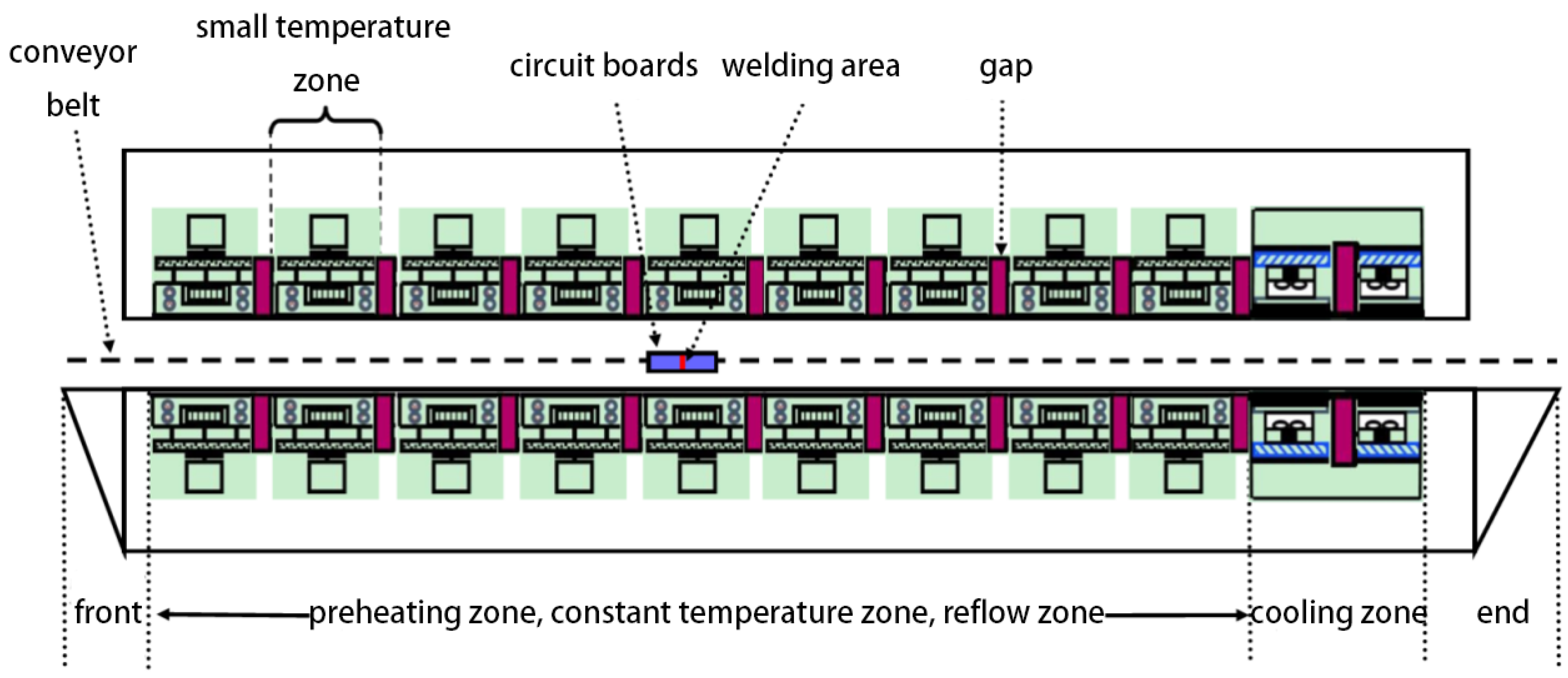
Several small temperature zones are set inside a reflow oven, which can be divided into four large temperature zones according to their functions: preheating zone, constant temperature zone, reflow zone, and cooling zone (shown in Figure 1). Both sides of the circuit board ride on the conveyor belt and enter the oven for heating and welding at a constant speed.

In this paper, the curve of furnace temperature is analyzed and studied by establishing a mechanism model that can reduce the number of experiments in actual production and obtain a better furnace temperature curve, thus improving production efficiency. Moreover, several concrete examples are given to discuss and solve some common problems in the industry.

2. Preparation and Establishment of the Model

2.1. Differential Model of Temperature Change in Welding Area

In the process of integrated circuit board soldering, the initial temperature of the circuit board is the indoor temperature. After the reflow oven is started, the air temperature in the oven reaches stability in a short time. After the temperature is stabilized, the circuit board enters the reflow oven on the conveyor belt at a constant speed. The temperature of each small temperature zone and the speed of the conveyor belt passing through the furnace are known. The derivative of the temperature of the circuit board with respect to time is the embodiment of the temperature rise and fall speed of the circuit board, and the rates of temperature increase and decrease are proportional to the difference between the circuit board and the ambient temperature. When the difference between the ambient temperature and the circuit board is large, the temperature of the circuit board changes quickly. When the difference decreases, the temperature changes slowly. Therefore, we use Newton’s law of cooling to study the relationship between the central temperature of the welding area and the temperature in the small temperature zone.

Taking the temperature of the welding area as the research object, the law of the furnace temperature curve is found from the angle of temperature change. It is known that the temperature of the welding area satisfies Newton’s law of cooling.

$$\frac{\mathrm{d}T}{\mathrm{d}t}=-k(T-C).$$

We will slightly modify this formula to facilitate the handling of problems. Let us assume that the temperature of the welding area is $T\left(t\right)$, and at this time, the circuit board is about to enter the reflow oven. Setting the front end of the oven area as the origin, x is the position of the welding area (preheating zone, constant temperature zone, reflow zone, and cooling zone); $C\left(x\right)$ is the ambient temperature of the welding area; and k is the influence coefficient reflecting the speed of temperature change, that is, k is the proportional coefficient of the heat loss per unit time of the object and the difference in the temperatures between the body and its environment. The position of the circuit board changes with time. Then, the ambient temperature around the welding area changes, which is influenced by the position of the circuit. The environmental temperature function is $C\left(x\right)$; the temperature change between temperature zones is continuous, and it represents the smooth curve in the image. Therefore, it is judged that it has the form of a piecewise smooth function as follows:

$$C\left(x\right)=\left\{\begin{array}{cc}{K}_1\left(x\right)\hfill & x\in [x_0,x_1),\hfill \\ T_1\hfill & x\in [x_1,x_2),\hfill \\ ⋮\hfill \\ K_n\left(x\right)\hfill & x\in [x_{2n-2},x_{2n-1}),\hfill \\ T_n\hfill & x\in [x_{2n-1},x_{2n}),\hfill \\ K_{n+1}\left(x\right)\hfill & x\in [x_{2n},x_{2n+1}].\hfill \end{array}\right.$$

where $T_i$$(i=1,2,\cdots n)$ is the center temperature zone of each small zone and $K_j\left(x\right)$$(j=1,2,\cdots ,n+1)$ represents the temperature of the area before and after the furnace and the gap. We represent the temperature in the center of each small temperature with $T_i$, and supplement the temperature data between the centers of two adjacent temperature zones using cubic interpolation in [24,25] to confirm function $C\left(x\right)$ of the whole interval. The specific construction method is shown in

Table 1. Construction method of ambient temperature.

Construction Method of $\mathit{C}\left(\mathit{x}\right)$
Step 1	For a small temperature area, its temperature is $T^{\prime }$, and we set the midpoint of the small temperature range as $x_0$; then, we intercept a small neighborhood $U(x_0,ϵ)(\forall ϵ>0)$ centered on this point. The figures of $C\left(x\right)$ in this neighborhood are defined as $T^{\prime }$.
Step 2	For two adjacent and small temperature zones a and b, and the gap between adjacent temperature zones, and for each small temperature zone, we choose the middle point and its neighborhood as in step 1, and respectively record them as $x_a,x_b,U(x_a,ϵ),$ and $U(x_b,ϵ)(\forall ϵ>0)$. According to $x_a$ and $x_b$, for interval $[x_a+ϵ,x_b-ϵ]$, we can carry out cubic interpolation to obtain temperature function $K^{\prime }\left(x\right)$ in this interval.
Step 3	Generally speaking, in a reflow oven, the set temperature of small temperature zone 1 is quite different from the temperature at the beginning of the furnace front area, but in order to conform to reality, the temperature change should be slow and continuous. We take the distance from the beginning of the furnace front area to the end of small temperature zone 1 as the buffer distance of the temperature change and record it as $[x_0,x_1)$. In this interval, according to the given temperature at both ends, $K_1\left(x\right)$ is obtained with the cubic interpolation method.
Step 4	In the same way as in step 3, because the set temperature of small temperature zone 10 and small temperature zone 11 is the same as the room temperature, the distance from the end of small temperature zone 9 to the end of the rear furnace zone is taken as the buffer zone of temperature change and is recorded as $[x_{2n},x_{2n+1}].$ Temperature $K_{n+1}\left(x\right)$ is obtained by means of cubic interpolation according to the given temperature at both ends. At the same time, $C\left(x\right)=K_{n+1}\left(x\right).$

.

From a physical point of view, this construction method can make the model more practical. The temperature in different temperature zones is different. The temperature zone in which the circuit board is currently located can be indicated by the speed and transmission time of the conveyor belt, which means that the position of soldering area x is function $x\left(t\right)=vt$, where v represents the speed of the conveyor belt. On the premise that time is measurable, the temperature zone of the circuit board is also known. The initial time is recorded as $t_0=0$; then, $C\left(x\right)$ and $K_j\left(x\right)$ can also be seen as functions $C^{\prime }\left(t\right)$ and $K^{\prime }\left(t\right)$, that is,

$$C^{\prime }\left(t\right)=C\left(x\left(t\right)\right),K_j^{\prime }\left(t\right)=K_j\left(x\left(t\right)\right),(j=1,2,\cdots ,n+1),$$

and under the condition of no ambiguity, the following uses mark $C^{\prime }\left(t\right)$ instead of $C\left(t\right).$

To sum up, our question lies in studying the mechanism model

$$\frac{\mathrm{d}T\left(t\right)}{\mathrm{d}t}=-k(T\left(t\right)-C\left(t\right)).$$

(1)

where $T\left(t\right)$ is the furnace temperature curve under study; k is the heat transfer coefficient, that is, k is the proportional coefficient of the heat loss per unit time of the object and the difference in the temperatures between the body and its environment; and $C\left(t\right)$ is the welding area at the time t ambient temperature of the location.

We set the corresponding temperature of every moment $t_i$ as $F\left(t_i\right)$, and $\Delta t_i=t_{i+1}-t_i$ is the time interval $(i=1,2,\cdots ,N)$. We write Equation (1) as the difference form as follows:

$$\frac{T_{i+1}-T_i}{\Delta t_i}=-k(T_i-C\left(t_i\right)),$$

also denoted as

$$T_{i+1}=T_i+k\Delta t_i(C\left(t_i\right)-T_i).$$

(2)

2.2. Determining Coefficient K Using Trial Solution

For each pending k, simulated furnace temperature curve $T\left(t\right)$ can be obtained with an iterative solution, which means that by changing Equation (2) to a difference equation satisfying the initial conditions, the difference equation can be solved with the Euler method in [25].

$$\left\{\begin{array}{c}{T}_{i+1}=T_i+k\Delta t_i(C\left(t_i\right)-T_i),\hfill \\ T_1=\theta .\hfill \end{array}\right.$$

where k is the coefficient and $\theta$ is the initial temperature. For each discrete point $t_i$, when the ambient temperature of the welding area, $C\left(t_i\right)$, is known and k is given, $T_{i+1}$ can be calculated by knowing $T_i(i=1,2,\cdots ,n-1)$. We can obtain all the corresponding results $T_n$ by means of iteration. It is easy to know each group $T_n$ defined by k, so it is function $T_n\left(k\right)$. Then, according to each $t_i$, we can find the corresponding appendix temperature data $F\left(t_i\right)$. When the variance of $T_n\left(k\right)$ and $F\left(t_i\right)$ is the smallest, it represents that the furnace temperature curve determined by k is best fitted with the furnace temperature curve given in the attachment, and what is required at this time is the optimal solution.

To sum up, the problem turns into seeking the best k, so that objective function Z is the smallest. At the same time,

$$Z=\sum _{i=1}^n{(F\left(t_i\right)-T_i\left(k\right))}^2.$$

3. Feasibility Test of the Model

In this section, we test the model with an example. We assume that the number of small temperature zones of the reflow oven is 11, the length of each small temperature zone is 30.5 cm, the gap between the small temperature zones is 5 cm, and the areas in front of and behind the reflow oven are 25 cm. The gap and the temperatures in front of and behind the oven do not need special treatment. Taking the furnace temperature curve drawn in an experiment as a reference, we establish a mathematical model and solve the problem according to the law of this temperature change. For the experimental data, we use the method described above to fit the temperature curve, and the steps are shown below.

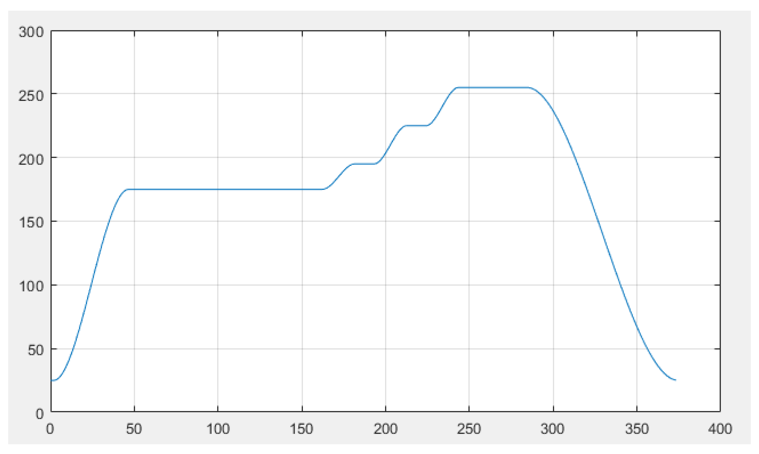
First, we construct function $C\left(t\right)$ according to

Table 2. Construction method of experimental ambient temperature.

Construction Method of $\mathit{C}\left(\mathit{t}\right)$
Step 1	The set temperature of small temperature zones 1~5 is 175 ${}^{°}$C; small temperature zone 1 is affected by the area in front of the furnace, and small temperature zone 5 is affected by small temperature zone 6, so we define function $C\left(t\right)$ in interval $[55.5,187.5)$. According to the given speed, $v=70\mathrm{cm}/\min$, we convert interval $[55.5,187.5)$ into the corresponding interval. We make the value of function $C\left(t\right)$ in the interval be equal to 175 ${}^{°}$C. Similarly, for small temperature zone 8 and small temperature zone 9, the interval of x is $[283.5,338.5)$. We convert it into the corresponding interval; then, the value of function $C\left(t\right)$ in the interval is 255 ${}^{°}$C.
Step 2	The set temperatures at the center of small temperature zones 6 and 7 are 195 ${}^{°}$C and 235 ${}^{°}$C. According to the relationship between x and t, we can obtain $C\left(t\right)$.
Step 3	For small temperature zone 1 and the furnace front zone, we manage our ambient temperature in the interval of $[0,55.5)$ using the cubic interpolated method according to the above method and obtain $C\left(t\right)$.
Step 4	For small temperature zones 10 and 11, and the area behind the furnace, our ambient temperature in interval $[338.5,435.5]$ is cubic-interpolated according to the above method, and we obtain $C\left(t\right)$.

.

So far, we have determined function $C\left(t\right)$. The result is shown in Figure 2. This figure shows the change in the set temperature in the area where the element is located as it moves over time.

Next, Equation (2) is rewritten into the following difference equation, which is solved with the Euler method:

$$\left\{\begin{array}{c}{\displaystyle T_{i+1}=T_i+\frac{k(C\left(t_i\right)-T_i)}{2},}\hfill \\ T_1=30.03.\hfill \end{array}\right.$$

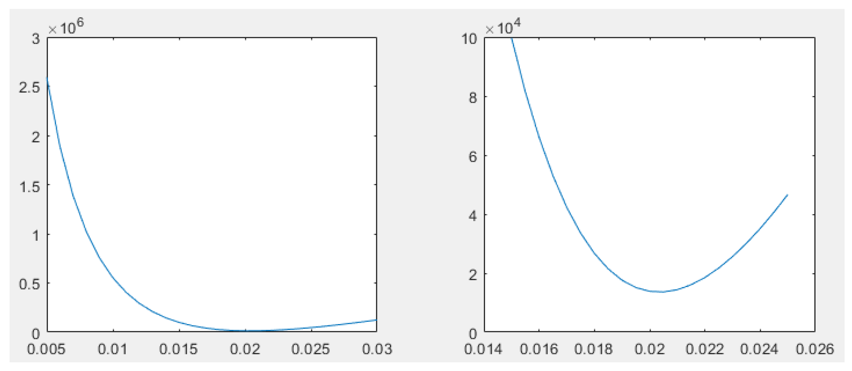
According to existing calculation studies, it can be preliminarily determined that k ranges in $[0.005,0.03]$. With k as the independent variable, we draw an image of the objective function, and the result is shown in Figure 3. This figure shows the change in error with the change in k.

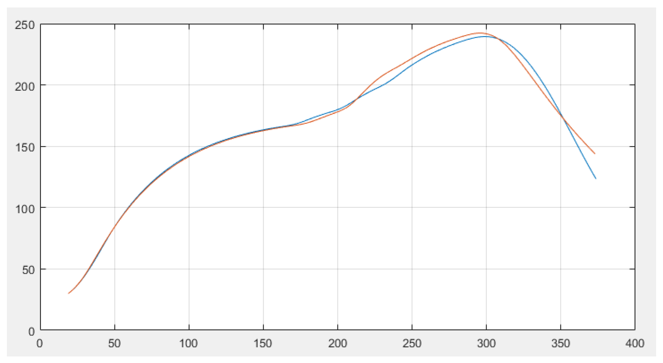
The k that gains the best condition is 0.021. We substitute the result into Formula (1) and solve $T\left(t\right)$. The comparison with the experimental data is shown in Figure 4.

It is found that the simulated curve is consistent with the actual curve, which proves that the model is reasonable.

4. Solutions to Common Problems in Several Industries

In this section, several concrete examples will be given to discuss and solve some common problems in the industry.

4.1. Drawing Furnace Temperature Curves in Different Temperature Environments

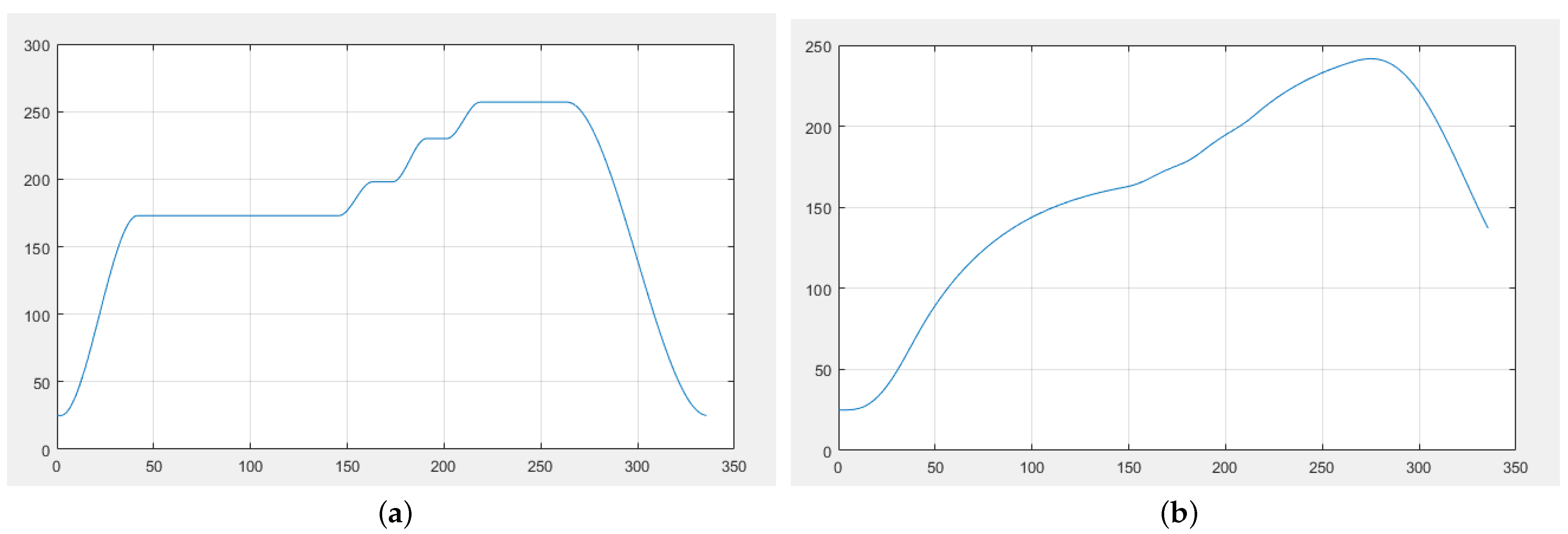
It is assumed that the conveying speed of the conveyor belt is 78 cm/min; the temperatures of small temperature zones 1~5 are all the same, 173 °C; the temperatures of small temperature zones 6 and 7 are 198 °C and 230 °C, respectively; small temperature zones 8 and 9 have the same temperature, 257 °C; and small temperature zones 10 and 11 have the same temperature, 25 °C. This chapter will next discuss the method application.

Following the discussion on k in the previous section, we substitute it into Equation (1). At this time, the relationship of temperature T of the welding area and time t is determined as

$$\frac{\mathrm{d}T\left(t\right)}{\mathrm{d}t}=-k(T\left(t\right)-C\left(t\right)).$$

According to the discussion, we only need to make the corresponding modification on $C\left(t\right)$, and the modified result is shown in Figure 5. This figure shows the temperature set for each temperature zone.

Then, we use two ways to solve problem $T\left(t\right)$, which are iteration and difference equations, to obtain the numerical solution. The obtained $T\left(t\right)$ is shown in Figure 5b. This figure shows the simulated furnace temperature curve. With this simulation, we can obtain some commonly used data in industrial production, which are shown in

Table 3. Simulation results.

Location	Temperature (°C)
Midpoint of zone 3	135.53
Midpoint of zone 6	179.36
Midpoint of zone 7	204.50
End of zone 8	225.12

. From this table, we can know the temperature around the element when it passes through the corresponding position.

4.2. Optimization of Furnace Speed

When reflow soldering circuit boards are running, the curve of furnace temperature needs to meet a certain condition, which is the process limit. Therefore, this chapter will discuss how to calculate the maximum transmission speed of the conveyor belt under the premise of not exceeding the process limit. The assumption we have is that the temperature in zones 1~5 is changed to 182 °C; in zone 6, the temperature is changed to 203 ${}^{°}$C; in zone 7, the temperature is changed to 237 °C; and in zones 8~9, it is changed to 254 °C. The rest of the situation remains the same as that in Section 4.1.

We assume that the requirements of $T\left(t\right)$ are the following:

• The temperature rising slope must not exceed 3.
• The temperature drop slope must not exceed 3.
• The time for the temperature to rise from 150 ${}^{°}$C to 190 ${}^{°}$C must be between 60 s and 120 s.
• The temperature above 217 ${}^{°}$C must be maintained for 40 s to 90 s.
• The highest temperature should be between 240 ${}^{°}$C and 250 ${}^{°}$C.

We summarize the above as four constraints of $T\left(t\right)$:

• ${\displaystyle \left|\frac{\mathrm{d}T\left(t\right)}{\mathrm{d}t}\right|\le 3}$.
• All satisfied $150\le T\left(t\right)\le 190$ of t compose interval $[t_{{\mathrm{s}}_1},t_{{\mathrm{e}}_1}]$, which satisfies $60\le |t_{{\mathrm{e}}_1}-t_{{\mathrm{s}}_1}|\le 120$.
• In all ascending segments, all t of $217\le T\left(t\right)$ meeting the requirements compose the interval of $[t_{{\mathrm{s}}_2},t_{{\mathrm{e}}_2}]$, which satisfies $40\le |t_{{\mathrm{e}}_2}-t_{{\mathrm{s}}_2}|\le 90$.
• Finally, $240\le maxT\left(t\right)\le 250$.

Using the above four constraints in $|t_{{\mathrm{e}}_1}-t_{{\mathrm{s}}_1}|$ and $|t_{{\mathrm{e}}_2}-t_{{\mathrm{s}}_2}|$, the model can be recorded as

$$\begin{array}{cc}\hfill & maxZ=v,\hfill \\ \hfill & \mathrm{s}.\mathrm{t}.\left\{\begin{array}{c}{\displaystyle \left|\frac{\mathrm{d}T\left(t\right)}{\mathrm{d}t}\right|\le 3,}\hfill \\ 240\le maxT\left(t\right)\le 250,\hfill \\ 60\le |t_{{\mathrm{e}}_1}-t_{{\mathrm{s}}_1}|\le 120,\hfill \\ 40\le |t_{{\mathrm{e}}_2}-t_{{\mathrm{s}}_2}|\le 90,\hfill \\ 65\le v\le 100.\hfill \end{array}\right.\hfill \end{array}$$

Through the preliminary test, conveyor belt speed v is optional in interval $[65,100]$, which is divided into M values, and we can obtain M data of conveyor belt speeds $v_i(i=1,2,\cdots ,M)$. Traversing data from large to small, the maximum furnace passing speed is found under this condition and is 83 cm/min.

4.3. Peak Temperature Coverage Problem

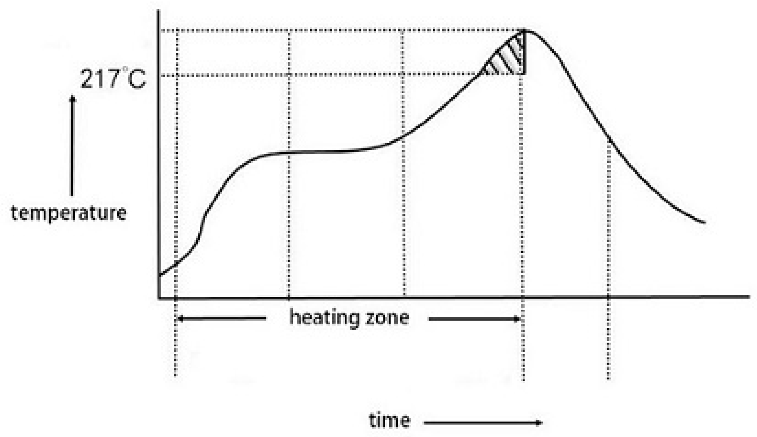
When welding, temperatures over 217 ${}^{°}$C in the welding area center should not be maintained for a long time, and the maximum temperature should not be too high.

The ideal condition is to minimize the area covered by the temperature curve over 217 ${}^{°}$C, as shown in Figure 6. Next, under this condition, we will discuss how to obtain the optimal furnace temperature curve, determine the temperature of each small temperature zone, determine the speed of the conveyor belt passing through the furnace, and obtain the mentioned area.

The area covered by the curve of the central temperature of the welding area exceeding 217 ${}^{°}$C and reaching the peak value of temperature can be divided. The approximate value of this area is calculated with the summation trapezoid method.

$${\int }_{t_1}^{t2}T\left(t\right)\mathrm{d}t\approx \sum \frac{T\left(t_i\right)+T\left(t_{i+1}\right)}{2}\Delta t.$$

The variable is speed v of the conveyor belt passing through the furnace, and the set temperature values of the temperature zones are $C_1,C_2,C_3,$ and $C_4$. From the previous discussion, we know that when a set of data are given as $v,C_1,C_2,C_3,$ and $C_4$, a boiler temperature curve $T\left(t\right)$ can be uniquely determined with Equation (1). According to boiler temperature curve $T\left(t\right)$, the required area of the shadow part can be obtained.

Considering the process boundary and that the temperature adjustment range of each temperature zone does not exceed 10 °C, the model can be recorded as

$$\begin{array}{cc}\hfill & minZ=\sum \frac{T\left(t_i\right)+T\left(t_{i+1}\right)}{2}\Delta t,\hfill \\ \hfill & \mathrm{s}.\mathrm{t}.\left\{\begin{array}{c}65\mathrm{cm}/\min \le v\le 100\mathrm{cm}/\min ,\hfill \\ \Delta C_i\le {10}^{°}\mathrm{C}(i=1,2,3,4),\hfill \\ T\left(t\right)\mathrm{meet}\mathrm{the}\mathrm{condition}.\hfill \end{array}\right.\hfill \end{array}$$

where Z in the objective function can be regarded as a multivariate function, i.e.,

$$Z=f(v,C_1,C_2,C_3,C_4).$$

If we want to consider every point of the global variable, it is quite difficult to solve it. Therefore, we choose the point-taking traversal method. According to the continuity of temperature change, we can pass, using discrete point-taking traversal, from low precision to fine precision (from large range to small range), find out the possible point of extreme value through step-by-step trial, and narrow the range for this point. Eventually, we can improve the accuracy of the ergodic solution step by step.

In this way, when there are enough cycles, we can obtain the corresponding optimal solution, $v,C_1,C_2,C_3,$ and $C_4$, of this problem. The results are shown in

Table 4. Simulation results.

Group	v (cm/min)	C1 (°C)	C2 (°C)	C3 (°C)	C4 (°C)	Area
The first group	74	165	185	229	255	39.94
The second group	74	165	187	229	255	39.94
The third group	74	165	189	227	255	39.94
The fourth and fifth groups	74	165	193	225	255	39.94

. The four groups of results all meet our expectations; the calculated areas are all 39.94, and their corresponding parameters are all optimal solutions.

4.4. Symmetry of Peak Temperature Image

When welding, in addition to meeting the process limit, it is also hoped that the furnace temperature curve, with the peak temperature as the center line and both sides exceeding 217 °C, is as symmetrical as possible (see Figure 6). In this paper, using Section 4.3, we will further find the local optimal solution in the vicinity of the optimal solution and obtain the corresponding optimal furnace temperature curve, the temperature set in each temperature zone, and the conveyor belt passing speed. Moreover, the corresponding index values will be given.

According to Formula (1), the furnace temperature curve image should satisfy

$$\frac{\mathrm{d}T}{\mathrm{d}t}=-k(T\left(t\right)-C\left(t\right)).$$

Assuming that the peak of $T\left(t\right)$ is reached at $t_{max}$, the furnace temperature curve should be symmetrical, with the peak temperature as the center line.

Let us take point $t_{\max }$ for central symmetry. Let us set the point to the left as $t_{-1},t_{-2},\cdots ,$ and take the right point as $t_1,t_2,\cdots$. Now, we just need to make

$$\sum {\left(T\left(t_{-i}\right)+T\left(t_i\right)\right)}^2$$

reach the minimum.

According to the previous discussion, when given a set of data, $v,C_1,C_2,C_3,$ and $C_4$, a furnace temperature curve $T\left(t\right)$ can be uniquely determined using Equation (1). According to furnace temperature curve $T\left(t\right)$, we can find the above variance.

To sum up, our problem comprises decision variables $v,C_1,C_2,C_3,$ and $C_4$, and objective function

$$Z=\sum {\left(T\left(t_{-i}\right)+T\left(t_i\right)\right)}^2.$$

Using Section 4.3, we only need to find the local optimal solution around the four groups of data given in Table 4.

Through calculation, when the objective function is the closest to the expected value, we obtain the results of calculation as shown in

Table 5. Simulation results.

Location	Calculation Result
Speed (cm/min)	75 cm/min
Set temperature of zones 1~5 (°C)	175 °C
Set temperature of zone 6 (°C)	189 °C
Set temperature of zone 7 (°C)	225 °C
Set temperature of zones 8~9 (°C)	255 °C
Area	42.21

below. This table shows the furnace passing speed and the set temperature of each temperature zone.

5. Summary

When an integrated circuit board is soldered in a reflow oven, temperature control seriously affects product quality. At present, temperature is mostly controlled and adjusted using experiments, and the establishment of this model provides a new idea to solve the problem. The mechanism model is used to monitor and control the temperature. According to Newton’s law of cooling, the relationship between the ambient temperature and the central temperature of the welding area is obtained. There is only one coefficient to be determined in this relationship. According to existing calculation studies, the optimal thermal conductivity coefficient is obtained with a tentative solution and numerical experiments, which greatly reduces the time complexity of the program and the loss in actual production. The thermal conductivity coefficient is substituted into the original model for operation. It can fit the furnace temperature curve given in the actual experiment well.

References

- Tang, Z.; Xie, B.; Liang, G. Control analysis of reflow furnace temperature curve. Electron. Qual. 2020, 15–19. [Google Scholar]
- Yao, X. Effect of plate feeding interval on furnace temperature curve. Shandong Ind. Technol. 2015, 271–272. [Google Scholar]
- Gong, Y. Study on temperature curve optimization of reflow welding furnace. Hot Work. Technol. 2013, 42, 187–190. [Google Scholar]
- Jun, F.; Ying, X.; Zeng, Y. Observe the temperature curve for solidification from high-speed video image. J. Therm. Anal. Calorim. 2021, 146, 1–5. [Google Scholar]
- Fradette, J. Real, Vacuum Furnace Temperature Measurement. Ind. Heat. 2015, 83, 52–59. [Google Scholar]
- Kurhade, A.; Rao, T.; Mathew, V. Effect of thermal conductivity of substrate board for temperature control of electronic components: A numerical study. Int. J. Mod. Phys. C 2021, 32, 1–12. [Google Scholar] [CrossRef]
- Li, H.; Li, R.; Wu, F. A New Control Performance Evaluation Based on LQG Benchmark for the Heating Furnace Temperature Control System. Processes 2020, 8, 1428. [Google Scholar] [CrossRef]
- Su, H.; Shi, J.; Ji, H. Investigating on the Iconic Gas Compositions Produced by Low-Temperature Heating Cotton. Symmetry 2020, 12, 883. [Google Scholar] [CrossRef]
- Yang, H.; Zou, L.; Song, Z.; Wang, X. Identification of the Ignition Point of High Voltage Cable Trenches Based on Ceiling Temperature Distribution. Symmetry 2022, 14, 1417. [Google Scholar] [CrossRef]
- Ahmad, I.; Jalil, A.; Ullah, A. Some new exact solutions of (4+1)-dimensional Davey-Stewartson-Kadomtsev-Petviashvili equation. Results Phys. 2023, 45, 106240. [Google Scholar] [CrossRef]
- Ahmad, S.; Saifullah, S.; Khan, A. Resonance, fusion and fission dynamics of bifurcation solitons and hybrid rogue wave structures of Sawada–Kotera equation. Commun. Nonlinear Sci. Numer. Simul. 2023, 119, 107117. [Google Scholar] [CrossRef]
- Alharbi, K.A.M.; Ullah, A. Ikramullah, Impact of viscous dissipation and coriolis effects in heat and mass transfer analysis of the 3D non-Newtonian fluid flow. Case Stud. Therm. Eng. 2022, 37, 102289. [Google Scholar] [CrossRef]
- Shah, Z.; Kumam, P.; Ullah, A. Mesoscopic Simulation for Magnetized Nanofluid Flow within a Permeable 3D Tank. IEEE Access 2021, 9, 135234–135244. [Google Scholar] [CrossRef]
- Naowarat, S.; Saifullah, S.; Ahmad, S. Periodic, Singular and Dark Solitons of a Generalized Geophysical KdV Equation by Using the Tanh-Coth Method. Symmetry 2023, 15, 135. [Google Scholar] [CrossRef]
- Khan, S.; Selim, M.M.; Khan, A. On the Analysis of the Non-Newtonian Fluid Flow Past a Stretching/Shrinking Permeable Surface with Heat and Mass Transfer. Coatings 2021, 11, 566. [Google Scholar] [CrossRef]
- Ullah, A.; Ikramullah; Selim, M.M. A Magnetite–Water-Based Nanofluid Three-Dimensional Thin Film Flow on an Inclined Rotating Surface with Non-Linear Thermal Radiations and Couple Stress Effects. Energies 2021, 14, 5531. [Google Scholar] [CrossRef]
- Ma, H. Study on Prediction and Optimization of Furnace Temperature Curve Based on Temperature Change Model. J. Phys. Conf. Ser. 2021, 1985, 012045. [Google Scholar] [CrossRef]
- Wang, X.; Sun, P.; Bai, H. Control model of Furnace Temperature Curve. J. Phys. Conf. Ser. 2021, 1903, 012030. [Google Scholar] [CrossRef]
- Febriardy, E.; Sutanto; Abimanyu, A. Development of PID-based furnace temperature control system for zirconium calcination. J. Phys. Conf. Ser. 2020, 1436, 012120. [Google Scholar] [CrossRef]
- Qiao, Y.; Zi, Y.; Song, Y. Research on Furnace Temperature Curve Based on Heat Convection and Heat Radiation. E3S Web Conf. 2021, 233, 04004. [Google Scholar]
- Zhang, J.; Jing, Y.; Chao, Y. Research on Furnace Temperature Curve. J. Phys. Conf. Ser. 2021, 2012, 012091. [Google Scholar] [CrossRef]
- Chen, H.; Luo, H.; Wu, S. Optimization of Furnace Temperature Curve Based on GA. IOP Conf. Ser. Earth Environ. Sci. 2021, 769, 1–23. [Google Scholar] [CrossRef]
- Cheng, Y.C. Optimization and simulation of furnace temperature curve based on heat. J. Phys. Conf. Ser. 2021, 1948, 012230. [Google Scholar]
- Zhao, J.; Dan, Q. Mathematical Modeling and Mathematical Experiment; Higher Education Press: Beijing, China, 2014. [Google Scholar]
- Li, Q.; Wang, N.; Yi, D. Numerical Analysis; Tsinghua University Press: Beijing, China, 2008. [Google Scholar]
Figure 1.
Sectional drawing of reflow furnace.
Figure 2.
Picture of ambient temperature.
Figure 3.
Variance when k is near 0.02.
Figure 4.
Simulation curves and experimental data.
Figure 5.
Simulation curves. (a) Ambient temperature; (b) temperature curve of reflow furnace.
Figure 6.
Area covered by peak temperature.