On Cohesive Fuzzy Sets, Operations and Properties with Applications in Electromagnetic Signals and Solar Activities

Abstract

In the present communication, a new concept of a cohesive fuzzy set (CHFS) has been proposed as a synchronized generalization of complex fuzzy sets and hesitant fuzzy sets in a systematic way. The novelty of the introduced notion lies in the selection of the best alternative among the available multiple favorable situations, where the possibility of its range is in the extended unit circle of the complex plane. We study the relationship between the CHFS and the complex intuitionistic fuzzy set (CIFS), along with validation of the obtained results. On the basis of the proposed notion, various properties, operations, and identities have been established with their necessary proof. The applications of CHFS in the process of filtering the signals for obtaining the reference signal using the necessary Fourier cosine transform or inverse Fourier cosine transform and identifying the maximum number of sunspots in a particular interval of solar activity have been suitably discussed with illustrative numerical examples. Some advantages of incorporating the proposed notion have also been tabulated for better understanding.

1. Introduction

Different researchers have designed various tools to solve the problems related to uncertainty inherent in our day-to-day lives, among which the probability theory and the theory of fuzzy sets are the most popular, as well as widely applicable. It may be noted that the information regarding the relative frequency has due concern with the probability theory, whereas, in the case of imprecise and inexact information having uncertainty for the decision makers, the fuzzy set theory is utilized. Zadeh, in 1965, introduced the concept of fuzzy sets (FSs) [1], which is found to be a more efficient decision aid technique, providing the ability to deal with the uncertainty and the vagueness present in our real-life problems. In the literature, it is prominently visible that the notion of fuzzy set theory plays a vital role in the areas of medical science [2], engineering applications [3], optimization [4], decision science [5], biological characterization problems [6], econometric [7], image analysis [8], nonsingleton fuzzy logic systems [9], machine learning approach for prediction [10], wireless sensor networks [11], memory array analysis [12], prioritization analysis [13], supervised machine learning techniques [14], classification of networks [15], etc. Moreover, Tang et al. [16] presented the algorithm of symmetry with the incorporation of intuitionistic fuzzy entropy and utilized it in the classification problem. Due to the increasing componential factor, Atanassov [17] introduced the concept of the intuitionistic fuzzy set (IFS), which includes membership, nonmembership, and hesitant function in the information. While working on the parametrization, it has been well established that the parametric versions of information measures provide better results in the technology of hydrogen fuel cells while deploying VIKOR and TOPSIS decision-making techniques [18]. Furthermore, the parametric form of information measures has been successfully applied in green supply chain management [19]. The parameterizations of attributes have also been successfully implemented in the renewable energy source selection problem with the incorporation of the matrix theory of picture fuzzy hypersoft information [20]. The notion of q-rung orthopair fuzzy sets has been in various decision-making fields [21,22,23,24,25].

In due course of time, several types of complexities were added upon, and researchers proposed various other generalizations of fuzzy sets and intuitionistic fuzzy sets. One of the major limitations of the application of FSs and IFSs is that these sets are not capable to address the periodicity occurring in some uncertain and incomplete/inexact information. In addition to this, various other problems having a two-dimensional framework cannot be modeled with FSs and IFSs. To counter this deficiency, Ramot et al. [26] extended the existing structure of the fuzzy set to a complex fuzzy set (CFS), which added the phase variable and also extended the range from [0, 1] to the unit circle in the complex plane, which spans the information in a wider sense. The membership function ${\mu }_S\left(x\right)=r_S\left(x\right)e^{i{w}_S\left(x\right)}$ in the complex fuzzy set implies that all the membership values must lie inside the unit circle on the complex plane. There is a kind of specific mapping between a CFS and Fourier transform which can be observed by restricting the range to a complex unit disk, henceforth having various applications in the field of communication systems, geological phenomena, optical systems, etc. Furthermore, Imtiaz et al. [27,28] extended the fuzzy sets to $\xi$-complex fuzzy sets with some of their important algebraic structural properties and extended them to group structures and fuzzy morphisms for image development. Recently, Sathiyaseelan et al. [29] presented the notion of symmetric matrices on the inverse soft expert sets and discussed various applications. Furthermore, several other applications are used in the fields of heart disease prediction [30], sensor communication [31], time series analysis [32], energy-efficient routing control [33], traveling enterprises [34], water channel estimator [35], and automation processes [36].

In the hesitant fuzzy set, the decision makers provide a set of various favorable (multifavorable situations) membership values for expressing their preferences/assessments at the same time. On the other hand, the complex fuzzy set provides freedom to add a phase component which enables us to gain information regarding a particular higher-dimensional periodic problem. Under the shadow of the above-stated discussions on the various generalizations and applications, we present a natural extension of the existing set to a novel concept of a cohesive fuzzy set (complex hesitant fuzzy set), which can explicitly focus on the set of the favorable situations for a particular uncertain higher-dimensional problem with the possible extended range of unit disk having a phase component. The phase component gives the advantage of addressing the impreciseness, which occurs periodically. The objective behind introducing the concept of CHFS is that it not only deals with the situation in which we are facing difficulty in choosing the best among the various favorable options but also helps in neglecting the unfavorable situations among the wide range of situations, which would certainly save both our time and energy.

Literature Review

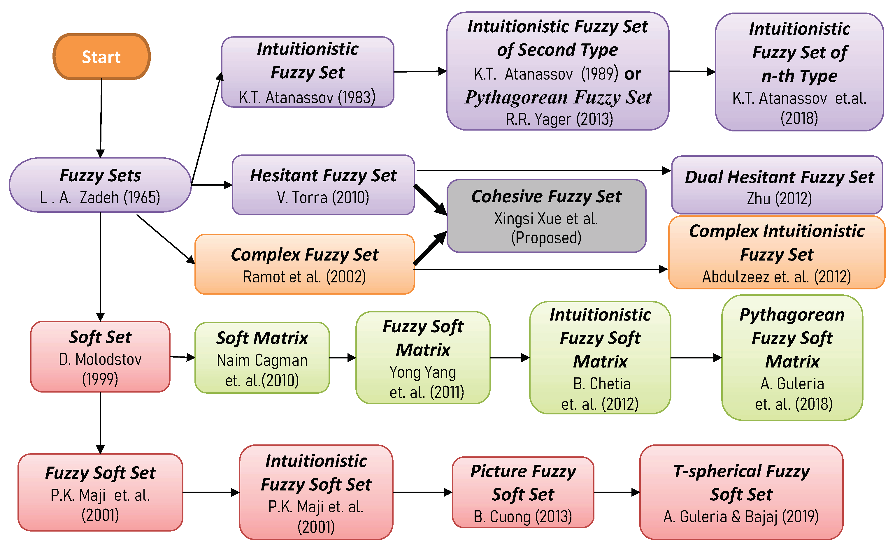
Torra [37] first introduced the notion of the hesitant fuzzy set (HFS) along with various operations (complement, union and intersection, etc.), which provided new dimensions to the research, especially in the field of group decision making, where the problem of multi-favorable situations can be better handled. For the sake of obtaining an overview of the various existing extensions and generalizations, we present an explanatory tree diagram in Figure 1 ([38,39,40,41,42,43,44,45,46,47,48,49,50]).

In addition to various generalizations of fuzzy sets stated above and their respective measures available in the literature, Xu and Xia [51] presented various distance measures, similarity measures, and correlation coefficients for hesitant fuzzy sets. Moreover, Torra [37] established a relation between HFS and IFS stating the enveloping procedure of IFS over HFS. Xu et al. [52] elaborated the hesitant fuzzy sets theoretically with different support systems and methodologies which have some kind of special advantageous features in the group decision-making processes. They also described the consensus process as the hesitant fuzzy setup to complete the decision-making process. Ren et al. [53] extended the concept of HFS to normal wiggly hesitant fuzzy sets to improve the rationality of the decision-making process and also proposed two introductory aggregation operators. Another important contribution made in the study of HFS is the dual hesitant fuzzy set (DHFS), which was proposed by Zhu et al. [54], in which the membership hesitancy function and nonmembership hesitancy function are used to support more flexible access to assign the values to each element in the domain. It may be noted that FS, IFS, and HFS can be treated as special cases of DHFS. Furthermore, Garg et al. [55] added the probability factor to DHFS and proposed the coefficients along with the weighted correlation coefficients for probabilistic dual hesitant fuzzy sets (PDHFSs). The CFS has been extended to a complex intuitionistic fuzzy set (CIFS) by Abdulzeez et al. [56], which added the complex membership and nonmembership function. Garg and Rani [57,58] contributed to two studies in the field of CIFS. First, they developed correlation/weighted correlation coefficients under the CIFS setup, where the membership degrees were utilized to represent the two-dimensional information. Secondly, they introduced and discussed the transformation relationships among the similarity, distance, entropies, and inclusion measures. Yaqoob et al. [59] introduced the notion of complex intuitionistic fuzzy graphs by combining two efficient theories (CIFS and graph theory) and also explained their advantage with the help of examples in the field of cellular network. In a study, Luqman et al. [60] discussed a detailed analysis on hypergraph representations of complex fuzzy information for a geometrical understanding. Moreover, Akram et al. [61] well presented a novel decision-making model utilizing the complex picture fuzzy Hamacher aggregation operators, and Mahmood et al. [62] proposed the notion of complex picture fuzzy N-soft sets with application in decision making.

The work in the present manuscript is organized as follows. Some standard definitions and preliminaries related to the further extensions of fuzzy sets are presented in Section 2. The notion of the cohesive fuzzy set (CHFS) is introduced with various operations, properties, and standard identities in Section 3. This extension of the fuzzy set is capable of dealing with situations in which there are multifavorable situations in the complex plane. In Section 4, we present the application of CHFS in the field of filtering the signals using the Fourier Cosine Transformation(FCT) and Inverse Discrete Fourier Cosine Transformation(IDFCT/DFCT). The detailed calculations for finding the reference signal by filtering the available ones are shown subsequently. In Section 5, the methodology of identifying the maximum number of sunspots in a particular interval under solar activity is presented with an example. The advantages and the limitations of the proposed methodology are listed in Section 6. Finally, the conclusions of the presented work are provided with the explanation and scope for future work in Section 7.

2. Preliminaries

In this section, for the sake of better readability, we provide the basic notions and definitions of hesitant fuzzy sets, complex fuzzy sets, and intuitionistic fuzzy sets, which are some important extensions of fuzzy sets introduced by Torra [37], Ramot et al. [26] and Atannassov [17] respectively. The hesitant fuzzy set is a fixed set of membership elements in [0, 1], whereas the IFSs set adds the membership and nonmembership functions to the fuzzy set. On the other hand, the complex fuzzy set (CFS) extends the range of FSs from a real number [0, 1] to the unit circle in a complex plane, which is very helpful in solving real-life problems, such as solar activity, containing phases as one more element. Here, we present the following definitions which are readily available in the literature:

Definition 1

((Fuzzy set) [1]). “Let A be set of uncertainty in a nonempty set X defined as

$$A=\{<x,{\mu }_A\left(x\right)>|x\in X\}$$

where ${\mu }_A\left(x\right)$ is a membership function in [0, 1].”

Definition 2

((Intuitionistic fuzzy set) [17]). “Let a fixed discourse X, an intuitionistic fuzzy set $A\subset X$ defined as:

$$A=\{<x,{\mu }_A\left(x\right),{\nu }_A\left(x\right)>|x\in X\}$$

where ${\mu }_A\left(x\right)$ and ${\nu }_A\left(x\right)$ are the degree of membership and nonmembership of element $x\in X$ in the interval [0, 1], respectively, with restrictions:

$$0\le {\mu }_A\left(x\right)+{\nu }_A\left(x\right)\le 1$$

and the degree of nondeterminacy ${\pi }_A\left(x\right)$, degree of favor ${\delta }_A\left(x\right)$, and degree of against ${\eta }_A\left(x\right)$ of the element $x\in X$ to A are defined as:

$$\begin{array}{c}\hfill \begin{array}{c}\hfill {\pi }_A\left(x\right)=1-{\mu }_A\left(x\right)-{\nu }_A\left(x\right)\\ \hfill {\delta }_A\left(x\right)={\mu }_A\left(x\right)+{\pi }_A\left(x\right)*{\mu }_A\left(x\right)\\ \hfill {\eta }_A\left(x\right)={\nu }_A\left(x\right)+{\pi }_A\left(x\right)*{\nu }_A\left(x\right)\end{array}\end{array}$$

and ${\pi }_A\left(x\right)=0$ for every $x\in X$ in case of ordinary fuzzy set.”

Definition 3

((Hesitant fuzzy set) [37]). “Let a fixed set be X, an HFS function in terms of hesitant fuzzy element (HFE) h on X that when applied to X returns a subset of [0, 1].

The mathematical symbol to express and understand the HFS easily is given by:

$$A=\{<x,h_A\left(x\right)>|x\in X\};$$

where $h_A\left(x\right)$ is a set of values denoting the degree of membership of element $x\in X$ in [0, 1].”

Given three HFEs represented by $h,h_1,$ and $h_2$, Torra [37] defined some operations on them, which can be described as

$$\begin{array}{c}\hfill \begin{array}{c}\hfill h^c={\cup }_{\gamma \in h}\{1-\gamma \};\\ \hfill h_1\cup h_2={\cup }_{{\gamma }_1\in h_1}{\cup }_{{\gamma }_2\in h_2}max\{{\gamma }_1,{\gamma }_2\};\\ \hfill h_1\cap h_2={\cup }_{{\gamma }_1\in h_1}{\cup }_{{\gamma }_2\in h_2}min\{{\gamma }_1,{\gamma }_2\}.\end{array}\end{array}$$

Definition 4

((Complex fuzzy set) [26]). (“Let a universe U, a complex fuzzy set S defined on discourse U characterized by a membership function ${\mu }_S\left(x\right)$ that assigns any element $x\in U$ a complex-valued grade of membership in S. By definition, the complex valued function ${\mu }_S\left(x\right)$ of the form $r_S\left(x\right){exp}^{i{w}_S\left(x\right)}$ lies within the unit circle in complex plane, where $i=\sqrt{-1},r_S\left(x\right)$ and $w_S\left(x\right)$ are both real valued, and $r_S\left(x\right)\in [0,1]$.”

The complex fuzzy set S is represented in the following form:

$$S=\left\{\left(x,{\mu }_S\left(x\right)\right)\right|x\in U\}.$$

Definition 5

((Complex intuitionistic fuzzy set) [56]). “Let a defined universe of discourse U, a complex intuitionistic fuzzy set S added the membership and nonmembership functions ${\mu }_S\left(x\right)$ and ${\gamma }_S\left(x\right)$ respectively to the complex fuzzy set, that assigns any element $x\in U$. This element x is a complex value element that contains both the membership and nonmembership values in S. According to the definition, it is already defined that the values of ${\mu }_S\left(x\right)$, ${\gamma }_S\left(x\right)$ and their sum will always lie in the unit circle in the complex plane, and the complex membership ${\mu }_S\left(x\right)$ and nonmembership ${\gamma }_S\left(x\right)$ functions are of the form $r_S\left(x\right){exp}^{i{w}_{{\mu }_S\left(x\right)}}$ and $k_S\left(x\right){exp}^{i{w}_{{\gamma }_S\left(x\right)}}$ respectively, where $i=\sqrt{-1}$,$w_{{\gamma }_S\left(x\right)}$ and $w_{{\mu }_S\left(x\right)}$ are real valued function.”

Moreover,

$$0\le r_S\left(x\right)\le 1,0\le k_S\left(x\right)\le 1,and0\le r_S\left(x\right)+k_S\left(x\right)\le 1.$$

Now, the CIFS is represented as

$$\begin{array}{c}\hfill \begin{array}{c}\hfill S=\{<x,{\mu }_S\left(x\right)=a,{\gamma }_S\left(x\right)=a^{\prime }>|x\in U\},where\\ \hfill {\mu }_S\left(x\right):U\to \left\{a\right|a\in C,\left|a\right|\le 1\},\\ \hfill {\gamma }_S\left(x\right):U\to \{a^{\prime }|a^{\prime }\in C,|a^{\prime }|\le 1\},\end{array}\end{array}$$

and $|{\mu }_S\left(x\right)+{\gamma }_S\left(x\right)|\le 1.$

3. Cohesive Fuzzy Sets, Operations, and Properties

In this section, we introduce the concept of a cohesive fuzzy set and provide its formal definition, along with various operations and related important properties.

The complex fuzzy set captures the phase component to process the information of a higher dimensional periodic problem, while in the theory of hesitant fuzzy set theory, experts provide a set of various multifavorable situations for presenting their assessments. In order to merge both requirements in a synchronized way, a natural extension to a set called a cohesive fuzzy set is introduced for explicitly focusing on the set of favorable situations for a particular uncertain higher-dimensional problem, with the possible extended range of unit disk having a phase component.

Definition 6

(Cohesive fuzzy set). Consider a fuzzy set T defined on a fixed universe of discourse S; a cohesive fuzzy set (CHFS) on T is in terms of function h when, applied on S, it returns a subset of unit circle, i.e.,

$$S_1=\{<x,h_T\left(x\right)>|x\in S\};$$

(1)

where $h_T$ is a complex set of values in a unit circle of the complex plane, denoting the possible membership degrees of elements $x\in S$ to the set $T\subset S$. Here, $h_T$ is of the form $r_T\left(x\right)exp\left(i{w}_T\left(x\right)\right)$, where $i=\sqrt{-1},r_T\left(x\right)$ and $w_T\left(x\right)$ both are real values and $r_T\left(x\right)\in [0,1].$

Example 1.

For understanding the basic structure of CHFS, let $S=\{x_1,x_2,x_3\}$ be the reference set. Suppose

$$h_{T_1}\left(x_1\right)=\{0.5exp\pi ,0.8exp\frac{\pi }{2},0.7exp\frac{\pi }{2}\},$$

$$h_{T_2}\left(x_2\right)=\{0.6exp\pi ,0.9exp\pi ,0.7exp\frac{\pi }{4}\},$$

and

$$h_{T_3}\left(x_3\right)=\{0.5exp\pi ,0.7exp\frac{\pi }{2},0.7exp\pi \}$$

denote the membership set of $x_i\left(i=1,2,3\right)$ to the set T, respectively. Then, the cohesive fuzzy set can be represented as

$$T=\{<x_1,\{0.5exp\pi ,0.8exp\frac{\pi }{2},0.7exp\frac{\pi }{2}\}>,$$

$$<x_2,\{0.6exp\pi ,0.9exp\pi ,0.7exp\frac{\pi }{4}\}>,<x_3,$$

$$\{0.5exp\pi ,0.7exp\frac{\pi }{2},0.7exp\pi \}>\}.$$

(2)

Various Basic Operations/Results on Cohesive Fuzzy Sets

Given a cohesive fuzzy set T whose membership function is given by $h_T$, we suitably propose its lower and upper bound as given below:

• lower bound: $h_T^{-}=min\left(h_T\right)$ and
• upper bound: $h_T^{+}=max\left(h_T\right)$.

It may be noted that the pair of complex hesitant functions $h_T^{-}$ and $1-h_T^{+}$ define the complex intuitionistic fuzzy set. Next, we first propose the definition of the complement of the cohesive fuzzy set as follows:

Definition 7

(Complement). Given a cohesive fuzzy set represented by membership function $h_T$, its complement set is defined as follows:

$$h_T^c={\cup }_{{\mu }_T\in h_T}{\left\{{\mu }_T\right\}}^c;$$

(3)

where ${\mu }_T=r_T{e}^{i{w}_T}$, i.e.,

$$h_T^c={\cup }_{{\mu }_T\in h_T}{\left\{{\mu }_T\right\}}^c={\cup }_{r_T\in h_T,w_T\in h_T}\left\{\left(1-r_T\right)e^{i\left(-w_T\right)}\right\}.$$

Proposition 1.

The operation of complement, i.e.,

$${\left(h_T^c\right)}^c=h_T$$

(4)

Proof. 

It is easy to observe that $\left(1-\left(1-r_T\right)\right)e^{i\left(-\left(-w_T\right)\right)}$ for all $r_T,w_T\in h_T$, hence the result. □

Definition 8

(Union). Suppose there are two cohesive fuzzy sets represented by their hesitant membership functions $h_{T_1}$ and $h_{T_2}$, respectively. The union of these CHFSs, denoted by $h_{T_1}\cup h_{T_2}$, can be defined as

$$\left(h_{T_1}\cup h_{T_2}\right)\left(x\right)=\{h_T\in \left(h_{T_1}\left(x\right)\cup h_{T_2}\left(x\right)\right)|h_T\ge max\left(h_{T_1}^{-},h_{T_2}^{-}\right)\}.$$

Definition 9

(Intersection). Suppose there are two cohesive fuzzy sets represented by their hesitant membership functions $h_{T_1}$ and $h_{T_2}$, respectively. The intersection of these CHFSs, denoted by $h_{T_1}\cap h_{T_2}$, can be defined as

$$\left(h_{T_1}\cap h_{T_2}\right)\left(x\right)=$$

$$\{h_T\in \left(h_{T_1}\left(x\right)\cap h_{T_2}\left(x\right)\right)|h_T\le min\left(h_{T_1}^{+},h_{T_2}^{+}\right)\}.$$

Hence, from the Definitions 7–9 given above, we write the following equations:

$$h_T^c={\cup }_{{\mu }_T\in h_T}{\left\{{\mu }_T\right\}}^c={\cup }_{r_T,w_T\in h_T}\left\{\left(1-r_T\right)e^{-i{w}_T}\right\};$$

$$h_{T_1}\cup h_{T_2}={\cup }_{{\mu }_{T_1}\in h_{T_1},{\mu }_{T_2}\in h_{T_2}}max\{{\mu }_{T_1},{\mu }_{T_2}\}$$

$$={\cup }_{r_T,w_T\in h_T}\{max\left(r_{T_1},r_{T_2}\right)e^{imax\left(w_{T_1},w_{T_2}\right)}\};$$

$$h_{T_1}\cap h_{T_2}={\cup }_{{\mu }_{T_1}\in h_{T_1},{\mu }_{T_2}\in h_{T_2}}min\{{\mu }_{T_1},{\mu }_{T_2}\}$$

$$={\cup }_{r_T,w_T\in h_T}\{min\left(r_{T_1},r_{T_2}\right)e^{imin\left(w_{T_1},w_{T_2}\right)}\}.$$

(5)

where ${\mu }_T,{\mu }_{T_1}$, and ${\mu }_{T_2}$ are of the form $r_T{e}^{i{w}_T},r_{T_1}{e}^{i{w}_{T_1}}$, and $r_{T_2}{e}^{i{w}_{T_2}}$, respectively.

Remark 1.

The CIFS contains complex membership and nonmembership functions, both as given in Definition 5. However, in the case of CHFS, only the complex membership function is considered. Therefore, we can say that every CHFS is contained in CIFS, whereas the reverse is not true.

Definition 10.

Suppose there is a cohesive fuzzy set given by$h_T$, we define CIFS$A_{env}\left(h_T\right)$as the envelope of$h_T$. Now, the set$A_{env}\left(h_T\right)$is represented by$<x,{\mu }_S\left(x\right),{\gamma }_S\left(x\right)>$with

$$\begin{array}{c}\hfill {\mu }_S\left(x\right)=min\left(h_T\right)=min\left({\mu }_T\right)\\ \hfill {\gamma }_S\left(x\right)=1-max\left(h_T\right)=1-max\left({\mu }_T\right)\end{array}$$

(6)

where ${\mu }_T=r_T{e}^{i{w}_T}$.

Proposition 2.

Now, the relationship between the cohesive fuzzy set and complex intuitionistic fuzzy set is given by

• $A_{env}\left(h_T^c\right)={\left(A_{env}\left(h_T\right)\right)}^c$;
• $A_{env}\left(h_{T_1}\cup h_{T_2}\right)=A_{env}\left(h_{T_1}\right)\cup A_{env}\left(h_{T_2}\right)$;
• $A_{env}\left(h_{T_1}\cap h_{T_2}\right)=A_{env}\left(h_{T_1}\right)\cap A_{env}\left(h_{T_2}\right)$.

Proof. 

We know that

$$A_{env}\left(h_T\right)=<minh\left(x\right),1-maxh\left(x\right)>$$

$$=<h_T^{-}\left(x\right),1-h_T^{+}\left(x\right)>$$

$${\left(A_{env}\left(h_T\right)\right)}^c=<1-h_T^{+}\left(x\right),h_T^{-}\left(x\right)>$$

and that

$$A_{env}\left(h_T^c\right)=<min{h}^c\left(x\right),1-max{h}^c\left(x\right)>$$

$$=<min\left(\left(1-r_T\left(x\right)\right)e^{-i{w}_T\left(x\right)}\right),1-max\left(\left(1-r_T\left(x\right)\right)e^{-i{w}_T\left(x\right)}\right)>$$

$$=<1-max\left(r_T\left(x\right)e^{i{w}_T\left(x\right)}\right),1-1+min\left(r_T\left(x\right)e^{i{w}_T\left(x\right)}\right)>$$

$$=<1-h_T^{+}\left(x\right),h_T^{-}\left(x\right)>$$

So, it proves the first inequality.

Then,

$$A_{env}\left(h_{T_1}\cup h_{T_2}\right)$$

$$=A_{env}\left(\{h_T\in \left(h_{T_1}\left(x\right)\cup h_{T_2}\left(x\right)\right)|h_T\ge max\left(h_{T_1}^{-},h_{T_2}^{-}\right)\}\right)$$

Thus, it implies that x lies in interval $[max\left(h_{T_1}^{-}\left(x\right),h_{T_2}^{-}\left(x\right)\right),max(h_{T_1}^{+}\left(x\right),h_{T_2}^{+}\left(x\right)]$. This implies that

$$A_{env}\left(h_{T_1}\cup h_{T_2}\right)=<max\left(h_{T_1}^{-},h_{T_2}^{-}\right),$$

$$min\left(1-h_{T_1}^{+},1-h_{T_2}^{+}\right)>$$

This proves the second inequality. □

Similarly, we can prove the third inequality. Finally, all the equalities are proved.

Next, for the sake of relative ordering over the cohesive fuzzy elements, some necessary comparing laws are provided as follows:

Definition 11.

For a given cohesive fuzzy element $h_T$,

$$f\left(h_T\right)=\frac{1}{\#h_T}\sum _{r_T,w_T\in h_T}{r}_T{e}^{i{w}_T}$$

is called the score function of $h_T$, where $\#h_T$ is the number of the elements in $h_T$.

For two cohesive fuzzy elements $h_{T_1}$ and $h_{T_2}$,

$$\mathrm{if}f\left(h_{T_1}\right)>f\left(h_{T_2}\right)\mathrm{then}{h}_{T_1}>h_{T_2};\mathrm{if}f\left(h_{T_1}\right)=f\left(h_{T_2}\right),$$

$then{h}_{T_1}=h_{T_2}.$

Next, we defined some new operations on the cohesive fuzzy elements $h_T,h_{T_1}$, and $h_{T_2}$ on the basis of the relations proposed in Proposition 2, which are given below:

• ${\left(h_T\right)}^{\lambda }={\cup }_{r_T,w_T\in h_T}{\left(r_T{e}^{i{w}_T}\right)}^{\lambda }$; where $\lambda \in \mathbb{R},\lambda >0$
• $\lambda h_T={\cup }_{r_T,w_T\in h_T}\left(1-{\left(1-r_T\right)}^{\lambda }\right)e^{i\lambda w_T}$
• (Direct Sum) $h_{T_1}\oplus h_{T_2}={\cup }_{r_{T_1},w_{T_1}\in h_{T_1},r_{T_2},w_{T_2}\in h_{T_2}}$
  $\left\{\left(r_{T_1}+r_{T_2}-r_{T_1}{r}_{T_2}\right)e^{i\left(w_{T_1}+w_{T_2}\right)}\right\}$
• (Direct Product) $h_{T_1}\otimes h_{T_2}={\cup }_{r_{T_1},w_{T_1}\in h_{T_1},r_{T_2},w_{T_2}\in h_{T_2}}$
  $\left\{\left(r_{T_1}{r}_{T_2}\right)e^{i\left(w_{T_1}+w_{T_2}\right)}\right\}$

Some more important operations have been established using the above operations on cohesive fuzzy elements as follows:

Theorem 1.

For the three given cohesive fuzzy elements $h_T,h_{T_1}$, and $h_{T_2}$, the following identities hold:

(1) ${h_{T_1}}^c\cup {h_{T_2}}^c={\left(h_{T_1}\cap h_{T_2}\right)}^c$.

(2) ${h_{T_1}}^c\cap {h_{T_2}}^c={\left(h_{T_1}\cup h_{T_2}\right)}^c$.

(3) ${\left(h_T^c\right)}^{\lambda }={\left(\lambda h_T\right)}^c$.

(4) $\lambda \left(h_T^c\right)={\left(h_T^{\lambda }\right)}^c$.

(5) $h_{T_1}^c\oplus h_{T_2}^c={\left(h_{T_1}\otimes h_{T_2}\right)}^c$.

(6) $h_{T_1}^c\otimes h_{T_2}^c={\left(h_{T_1}\oplus h_{T_2}\right)}^c$.

Proof. 

The proof for the above-stated identities is outlined below:

(1) ${h_{T_1}}^c\cup {h_{T_2}}^c={\cup }_{\begin{array}{c}{r}_{T_1},w_{T_1}\in h_{T_1}\end{array}{r}_{T_1},w_{T_1}\in h_{T_1}}$

$max\left(\left(1-r_{T_1}\right)e^{-i{w}_{T_1}},\left(1-r_{T_2}\right)e^{-i{w}_{T_2}}\right)$

$=\left(1-min\left(r_{T_1},r_{T_2}\right)\right)e^{-i\left(1-min\left(w_{T_1},w_{T_2}\right)\right)}$

$={\left(h_{T_1}\cap h_{T_2}\right)}^c$.

(2) ${h_{T_1}}^c\cap {h_{T_2}}^c={\cup }_{\begin{array}{c}{r}_{T_1},w_{T_1}\in h_{T_1}\end{array}{r}_{T_1},w_{T_1}\in h_{T_1}}$

$min\left(\left(1-r_{T_1}\right)e^{-i{w}_{T_1}},\left(1-r_{T_2}\right)e^{-i{w}_{T_2}}\right)$

$=\left(1-max\left(r_{T_1},r_{T_2}\right)\right)e^{-i\left(1-max\left(w_{T_1},w_{T_2}\right)\right)}$

$={\left(h_{T_1}\cup h_{T_2}\right)}^c$.

(3) ${\left(h_T^c\right)}^{\lambda }={\cup }_{r_T,w_T\in h_T}{\left(\left(1-r_T\right)e^{-i{w}_T}\right)}^{\lambda }$

$={\cup }_{r_T,w_T\in h_T}{\left(1-r_T\right)}^{\lambda }{e}^{-i\lambda w_T}$

$={\cup }_{r_T,w_T\in h_T}{\left(\left(1-{\left(1-r_T\right)}^{\lambda }\right)e^{i\lambda w_T}\right)}^c$

$={\left(\lambda h_T\right)}^c$.

(4) $\lambda \left(h_T^c\right)={\cup }_{r_T,w_T\in h_T}\left(1-\left(1-{\left(1-r_T\right)}^{\lambda }\right)\right)e^{-i\lambda w_T}={\left(h_T^{\lambda }\right)}^c$.

(5) $h_{T_1}^c\oplus h_{T_2}^c$=${\cup }_{r_{T_1},w_{T_1}\in h_{T_1},r_{T_2},w_{T_2}\in h_{T_2}}$$\left\{\left(\left(1-r_{T_1}\right)+\left(1-r_{T_2}\right)-\left(1-r_{T_1}\right)\left(1-r_{T_2}\right)\right)e^{-i\left(w_{T_1}+w_{T_2}\right)}\right\}$$$

$={\cup }_{r_{T_1},w_{T_1}\in h_{T_1},r_{T_2},w_{T_2}\in h_{T_2}}\left\{\left(1-r_{T_1}{r}_{T_2}\right)e^{-i\left(w_{T_1}+w_{T_2}\right)}\right\}$

$={\left(h_{T_1}\otimes h_{T_2}\right)}^c$.

(6) $h_{T_1}^c\otimes h_{T_2}^c=$${\cup }_{r_{T_1},w_{T_1}\in h_{T_1},r_{T_2},w_{T_2}\in h_{T_2}}\left\{\left(1-r_{T_1}\right)\left(1-r_{T_2}\right)e^{-i\left(w_{T_1}+w_{T_2}\right)}\right\}$

$={\cup }_{r_{T_1},w_{T_1}\in h_{T_1},r_{T_2},w_{T_2}\in h_{T_2}}\{\left(1-\left(r_{T_1}+r_{T_2}-r_{T_1}{r}_{T_2}\right)\right)$$e^{-i\left(w_{T_1}+w_{T_2}\right)}\}$

$={\left(h_{T_1}\oplus h_{T_2}\right)}^c$. □

Definition 12.

Let $h_{T_1}$ and $h_{T_2}$ be two cohesive fuzzy elements; we propose the operators given below:

(1) $h_{T_1}{o}_1{h}_{T_2}={\cup }_{{\mu }_{T_1}\in h_{T_1}}\left\{\frac{|{\mu }_{T_1}-{\mu }_{T_2}|}{1+|{\mu }_{T_1}-{\mu }_{T_2}|}\right\}$

(2) $h_{T_1}{o}_2{h}_{T_2}={\cup }_{{\mu }_{T_1}\in h_{T_1}}\left\{\frac{|{\mu }_{T_1}-{\mu }_{T_2}|}{1+2|{\mu }_{T_1}-{\mu }_{T_2}|}\right\}$

(3) $h_{T_1}{o}_3{h}_{T_2}={\cup }_{{\mu }_{T_1}\in h_{T_1}}\left\{\frac{|{\mu }_{T_1}-{\mu }_{T_2}|}{2}\right\}$

(4) $h_{T_1}{o}_4{h}_{T_2}={\cup }_{{\mu }_{T_1}\in h_{T_1}}\left\{\frac{|{\mu }_{T_1}.{\mu }_{T_2}|}{2}\right\}$

where ${\mu }_{T_1}$ and ${\mu }_{T_2}$ are in the form of $r_{T_1}{e}^{i{w}_{T_1}}$ and $r_{T_2}{e}^{i{w}_{T_2}}$, respectively.

Remark 2.

The following may be observed from the above definition:

• $h_{T_1}\oplus h_{T_2}={\cup }_{r_{T_1},w_{T_1}\in h_{T_1},r_{T_2},w_{T_2}\in h_{T_2}}$
  $\left\{\left(r_{T_1}+r_{T_2}-r_{T_1}{r}_{T_2}\right)e^{i\left(w_{T_1}+w_{T_2}\right)}\right\}$
  $={\cup }_{{\mu }_{T_1},w_{T_1}\in h_{T_1},{\mu }_{T_2},w_{T_2}\in h_{T_2}}\{{\mu }_{T_1}{e}^{i{w}_{T_2}}+{\mu }_{T_2}{e}^{i{w}_{T_1}}-{\mu }_{T_1}{\mu }_{T_2}\}$.
• $h_{T_1}\otimes h_{T_2}={\cup }_{r_{T_1},w_{T_1}\in h_{T_1},r_{T_2},w_{T_2}\in h_{T_2}}$
  $\left\{\left(r_{T_1}{r}_{T_2}\right)e^{i\left(w_{T_1}+w_{T_2}\right)}\right\}$
  $={\cup }_{{\mu }_{T_1}\in h_{T_1},{\mu }_{T_2}\in h_{T_2}}\left\{{\mu }_{T_1}{\mu }_{T_2}\right\}$.

Theorem 2.

With$h_{T_1}$ and $h_{T_2}$ being the two cohesive fuzzy elements, we have the following identities:

(1) $\left(h_{T_1}\oplus h_{T_2}\right)\cap \left(h_{T_1}{o}_1{h}_{T_2}\right)=\left(h_{T_1}{o}_1{h}_{T_2}\right)$;

(2) $\left(h_{T_1}\oplus h_{T_2}\right)\cup \left(h_{T_1}{o}_1{h}_{T_2}\right)=\left(h_{T_1}\oplus h_{T_2}\right)$;

(3) $\left(h_{T_1}\otimes h_{T_2}\right)\cap \left(h_{T_1}{o}_1{h}_{T_2}\right)=\left(h_{T_1}{o}_1{h}_{T_2}\right)$;

(4) $\left(h_{T_1}\otimes h_{T_2}\right)\cap \left(h_{T_1}{o}_1{h}_{T_2}\right)=\left(h_{T_1}\otimes h_{T_2}\right)$;

(5) $\left(h_{T_1}\oplus h_{T_2}\right)\cap \left(h_{T_1}{o}_2{h}_{T_2}\right)=\left(h_{T_1}{o}_2{h}_{T_2}\right)$;

(6) $\left(h_{T_1}\oplus h_{T_2}\right)\cup \left(h_{T_1}{o}_2{h}_{T_2}\right)=\left(h_{T_1}\oplus h_{T_2}\right)$;

(7) $\left(h_{T_1}\otimes h_{T_2}\right)\cap \left(h_{T_1}{o}_2{h}_{T_2}\right)=\left(h_{T_1}{o}_2{h}_{T_2}\right)$;

(8) $\left(h_{T_1}\otimes h_{T_2}\right)\cap \left(h_{T_1}{o}_2{h}_{T_2}\right)=\left(h_{T_1}\otimes h_{T_2}\right)$;

(9) $\left(h_{T_1}\oplus h_{T_2}\right)\cap \left(h_{T_1}{o}_3{h}_{T_2}\right)=\left(h_{T_1}{o}_3{h}_{T_2}\right)$;

(10) $\left(h_{T_1}\oplus h_{T_2}\right)\cup \left(h_{T_1}{o}_3{h}_{T_2}\right)=\left(h_{T_1}\oplus h_{T_2}\right)$;

(11) $\left(h_{T_1}\otimes h_{T_2}\right)\cap \left(h_{T_1}{o}_3{h}_{T_2}\right)=\left(h_{T_1}{o}_3{h}_{T_2}\right)$;

(12) $\left(h_{T_1}\otimes h_{T_2}\right)\cap \left(h_{T_1}{o}_3{h}_{T_2}\right)=\left(h_{T_1}\otimes h_{T_2}\right)$;

(13) $\left(h_{T_1}\oplus h_{T_2}\right)\cap \left(h_{T_1}{o}_4{h}_{T_2}\right)=\left(h_{T_1}{o}_4{h}_{T_2}\right)$;

(14) $\left(h_{T_1}\oplus h_{T_2}\right)\cup \left(h_{T_1}{o}_4{h}_{T_2}\right)=\left(h_{T_1}\oplus h_{T_2}\right)$;

(15) $\left(h_{T_1}\otimes h_{T_2}\right)\cap \left(h_{T_1}{o}_4{h}_{T_2}\right)=\left(h_{T_1}{o}_4{h}_{T_2}\right)$;

(16) $\left(h_{T_1}\otimes h_{T_2}\right)\cap \left(h_{T_{11}}{o}_4{h}_{T_2}\right)=\left(h_{T_1}\otimes h_{T_2}\right).$

Proof. 

All the above-listed properties were proven one by one. In view of Definition 12 stated above, we have

(1) $\left(h_{T_1}\oplus h_{T_2}\right)\cap \left(h_{T_1}{o}_1{h}_{T_2}\right)$

$=\left({\cup }_{\begin{array}{c}{\mu }_{T_1},w_{T_1}\in h_{T_1}\\ {\mu }_{T_2},w_{T_2}\in h_{T_2}\end{array}}\{{\mu }_{T_1}{e}^{i{w}_{T_2}}+{\mu }_{T_2}{e}^{i{w}_{T_1}}-{\mu }_{T_1}{\mu }_{T_2}\}\right)\cap \left({\cup }_{\begin{array}{c}{\mu }_{T_1}\in h_{T_1}\\ {\mu }_{T_2}\in h_{T_2}\end{array}}\left\{\frac{|{\mu }_{T_1}-{\mu }_{T_2}|}{1+|{\mu }_{T_1}-{\mu }_{T_2}|}\right\}\right)$

$={\cup }_{\begin{array}{c}{\mu }_{T_1},w_{T_1}\in h_{T_1}\\ {\mu }_{T_2},w_{T_2}\in h_{T_2}\end{array}}min$

$\{{\mu }_{T_1}{e}^{i{w}_{T_2}}+{\mu }_{T_2}{e}^{i{w}_{T_1}}-{\mu }_{T_1}{\mu }_{T_2},\frac{|{\mu }_{T_1}-{\mu }_{T_2}|}{1+|{\mu }_{T_1}-{\mu }_{T_2}|}\}$

$={\cup }_{\begin{array}{c}{\mu }_{T_1}\in h_{T_1}\\ {\mu }_{T_2}\in h_{T_2}\end{array}}\left\{\frac{|{\mu }_{T_1}-{\mu }_{T_2}|}{1+|{\mu }_{T_1}-{\mu }_{T_2}|}\right\}$$=\left(h_{T_1}{o}_1{h}_{T_2}\right)$.

(2) $\left(h_{T_1}\oplus h_{T_2}\right)\cup \left(h_{T_1}{o}_1{h}_{T_2}\right)$

$=\left({\cup }_{\begin{array}{c}{\mu }_{T_1},w_{T_1}\in h_{T_1}\\ {\mu }_{T_2},w_{T_2}\in h_{T_2}\end{array}}\{{\mu }_{T_1}{e}^{i{w}_{T_2}}+{\mu }_{T_2}{e}^{i{w}_{T_1}}-{\mu }_{T_1}{\mu }_{T_2}\}\right)\cup \left({\cup }_{\begin{array}{c}{\mu }_{T_1}\in h_{T_1}\\ {\mu }_{T_2}\in h_{T_2}\end{array}}\left\{\frac{|{\mu }_{T_1}-{\mu }_{T_2}|}{1+|{\mu }_{T_1}-{\mu }_{T_2}|}\right\}\right)$

$={\cup }_{\begin{array}{c}{\mu }_{T_1},w_{T_1}\in h_{T_1}\\ {\mu }_{T_2},w_{T_2}\in h_{T_2}\end{array}}max\{{\mu }_{T_1}{e}^{i{w}_{T_2}}+{\mu }_{T_2}{e}^{i{w}_{T_1}}-{\mu }_{T_1}{\mu }_{T_2},$

$\frac{|{\mu }_{T_1}-{\mu }_{T_2}|}{1+|{\mu }_{T_1}-{\mu }_{T_2}|}\}$

$={\cup }_{\begin{array}{c}{\mu }_{T_1},w_{T_1}\in h_{T_1}\\ {\mu }_{T_2},w_{T_2}\in h_{T_2}\end{array}}\{{\mu }_{T_1}{e}^{i{w}_{T_2}}+{\mu }_{T_2}{e}^{i{w}_{T_1}}-{\mu }_{T_1}{\mu }_{T_2}\}$

$=\left(h_{T_1}\oplus h_{T_2}\right)$.

(3) $\left(h_{T_1}\otimes h_{T_2}\right)\cap \left(h_{T_1}{o}_1{h}_{T_2}\right)$

$=\left({\cup }_{\begin{array}{c}{\mu }_{T_1}\in h_{T_1}\\ {\mu }_{T_2}\in h_{T_2}\end{array}}\left\{{\mu }_{T_1}{\mu }_{T_2}\right\}\right)\cap \left({\cup }_{\begin{array}{c}{\mu }_{T_1}\in h_{T_1}\\ {\mu }_{T_2}\in h_{T_2}\end{array}}\left\{\frac{|{\mu }_{T_1}-{\mu }_{T_2}|}{1+|{\mu }_{T_1}-{\mu }_{T_2}|}\right\}\right)$

$={\cup }_{\begin{array}{c}{\mu }_{T_1}\in h_{T_1}\\ {\mu }_{T_2}\in h_{T_2}\end{array}}min\{{\mu }_{T_1}{\mu }_{T_2},\frac{|{\mu }_{T_1}-{\mu }_{T_2}|}{1+|{\mu }_{T_1}-{\mu }_{T_2}|}\}$

$={\cup }_{\begin{array}{c}{\mu }_{T_1}\in h_{T_1}\\ {\mu }_{T_2}\in h_{T_2}\end{array}}\left\{\frac{|{\mu }_{T_1}-{\mu }_{T_2}|}{1+|{\mu }_{T_1}-{\mu }_{T_2}|}\right\}$$=\left(h_{T_1}{o}_1{h}_{T_2}\right)$.

(4) $\left(h_{T_1}\otimes h_{T_2}\right)\cup \left(h_{T_1}{o}_1{h}_{T_2}\right)$

$=\left({\cup }_{\begin{array}{c}{\mu }_{T_1}\in h_{T_1}\\ {\mu }_{T_2}\in h_{T_2}\end{array}}\left\{{\mu }_{T_1}{\mu }_{T_2}\right\}\right)\cup \left({\cup }_{\begin{array}{c}{\mu }_{T_1}\in h_{T_1}\\ {\mu }_{T_2}\in h_{T_2}\end{array}}\left\{\frac{|{\mu }_{T_1}-{\mu }_{T_2}|}{1+|{\mu }_{T_1}-{\mu }_{T_2}|}\right\}\right)$

$={\cup }_{\begin{array}{c}{\mu }_{T_1}\in h_{T_1}\\ {\mu }_{T_2}\in h_{T_2}\end{array}}max\{{\mu }_{T_1}{\mu }_{T_2},\frac{|{\mu }_{T_1}-{\mu }_{T_2}|}{1+|{\mu }_{T_1}-{\mu }_{T_2}|}\}$

$={\cup }_{\begin{array}{c}{\mu }_{T_1}\in h_{T_1}\\ {\mu }_{T_2}\in h_{T_2}\end{array}}\left\{{\mu }_{T_1}{\mu }_{T_2}\right\}$$=\left(h_{T_1}\otimes h_{T_2}\right)$.

(5) $\left(h_{T_1}\oplus h_{T_2}\right)\cap \left(h_{T_1}{o}_2{h}_{T_2}\right)$

$=\left({\cup }_{\begin{array}{c}{\mu }_{T_1},w_{T_1}\in h_{T_1}\\ {\mu }_{T_2},w_{T_2}\in h_{T_2}\end{array}}\{{\mu }_{T_1}{e}^{i{w}_{T_2}}+{\mu }_{T_2}{e}^{i{w}_{T_1}}-{\mu }_{T_1}{\mu }_{T_2}\}\right)\cap \left({\cup }_{\begin{array}{c}{\mu }_{T_1}\in h_{T_1}\\ {\mu }_{T_2}\in h_{T_2}\end{array}}\left\{\frac{|{\mu }_{T_1}-{\mu }_{T_2}|}{1+2|{\mu }_{T_1}-{\mu }_{T_2}|}\right\}\right)$

$={\cup }_{\begin{array}{c}{\mu }_{T_1},w_{T_1}\in h_{T_1}\\ {\mu }_{T_2},w_{T_2}\in h_{T_2}\end{array}}$

$min\{{\mu }_{T_1}{e}^{i{w}_{T_2}}+{\mu }_{T_2}{e}^{i{w}_{T_1}}-{\mu }_{T_1}{\mu }_{T_2},\frac{|{\mu }_{T_1}-{\mu }_{T_2}|}{1+2|{\mu }_{T_1}-{\mu }_{T_2}|}\}$

$={\cup }_{\begin{array}{c}{\mu }_{T_1}\in h_{T_1}\\ {\mu }_{T_2}\in h_{T_2}\end{array}}\left\{\frac{|{\mu }_{T_1}-{\mu }_{T_2}|}{1+2|{\mu }_{T_1}-{\mu }_{T_2}|}\right\}$$=\left(h_{T_1}{o}_2{h}_{T_2}\right)$.

(6) $\left(h_{T_1}\oplus h_{T_2}\right)\cup \left(h_{T_1}{o}_2{h}_{T_2}\right)$

$=\left({\cup }_{\begin{array}{c}{\mu }_{T_1},w_{T_1}\in h_{T_1}\\ {\mu }_{T_2},w_{T_2}\in h_{T_2}\end{array}}\{{\mu }_{T_1}{e}^{i{w}_{T_2}}+{\mu }_{T_2}{e}^{i{w}_{T_1}}-{\mu }_{T_1}{\mu }_{T_2}\}\right)\cup \left({\cup }_{\begin{array}{c}{\mu }_{T_1}\in h_{T_1}\\ {\mu }_{T_2}\in h_{T_2}\end{array}}\left\{\frac{|{\mu }_{T_1}-{\mu }_{T_2}|}{1+2|{\mu }_{T_1}-{\mu }_{T_2}|}\right\}\right)$

$={\cup }_{\begin{array}{c}{\mu }_{T_1},w_{T_1}\in h_{T_1}\\ {\mu }_{T_2},w_{T_2}\in h_{T_2}\end{array}}max\{{\mu }_{T_1}{e}^{i{w}_{T_2}}+{\mu }_{T_2}{e}^{i{w}_{T_1}}-{\mu }_{T_1}{\mu }_{T_2},$

$\frac{|{\mu }_{T_1}-{\mu }_{T_2}|}{1+2|{\mu }_{T_1}-{\mu }_{T_2}|}\}$

$={\cup }_{\begin{array}{c}{\mu }_{T_1},w_{T_1}\in h_{T_1}\\ {\mu }_{T_2},w_{T_2}\in h_{T_2}\end{array}}\{{\mu }_{T_1}{e}^{i{w}_{T_2}}+{\mu }_{T_2}{e}^{i{w}_{T_1}}-{\mu }_{T_1}{\mu }_{T_2}\}$

$=\left(h_{T_1}\oplus h_{T_2}\right)$.

(7) $\left(h_{T_1}\otimes h_{T_2}\right)\cap \left(h_{T_1}{o}_2{h}_{T_2}\right)$

$=\left({\cup }_{\begin{array}{c}{\mu }_{T_1}\in h_{T_1}\\ {\mu }_{T_2}\in h_{T_2}\end{array}}\left\{{\mu }_{T_1}{\mu }_{T_2}\right\}\right)\cap \left({\cup }_{\begin{array}{c}{\mu }_{T_1}\in h_{T_1}\\ {\mu }_{T_2}\in h_{T_2}\end{array}}\left\{\frac{|{\mu }_{T_1}-{\mu }_{T_2}|}{1+2|{\mu }_{T_1}-{\mu }_{T_2}|}\right\}\right)$

$={\cup }_{\begin{array}{c}{\mu }_{T_1}\in h_{T_1}\\ {\mu }_{T_2}\in h_{T_2}\end{array}}min\{{\mu }_{T_1}{\mu }_{T_2},\frac{|{\mu }_{T_1}-{\mu }_{T_2}|}{1+2|{\mu }_{T_1}-{\mu }_{T_2}|}\}$

$={\cup }_{\begin{array}{c}{\mu }_{T_1}\in h_{T_1}\\ {\mu }_{T_2}\in h_{T_2}\end{array}}\left\{\frac{|{\mu }_{T_1}-{\mu }_{T_2}|}{1+2|{\mu }_{T_1}-{\mu }_{T_2}|}\right\}$$=\left(h_{T_1}{o}_2{h}_{T_2}\right)$.

(8) $\left(h_{T_1}\otimes h_{T_2}\right)\cup \left(h_{T_1}{o}_2{h}_{T_2}\right)$

$=\left({\cup }_{\begin{array}{c}{\mu }_{T_1}\in h_{T_1}\\ {\mu }_{T_2}\in h_{T_2}\end{array}}\left\{{\mu }_{T_1}{\mu }_{T_2}\right\}\right)\cup \left({\cup }_{\begin{array}{c}{\mu }_{T_1}\in h_{T_1}\\ {\mu }_{T_2}\in h_{T_2}\end{array}}\left\{\frac{|{\mu }_{T_1}-{\mu }_{T_2}|}{1+2|{\mu }_{T_1}-{\mu }_{T_2}|}\right\}\right)$

$={\cup }_{\begin{array}{c}{\mu }_{T_1}\in h_{T_1}\\ {\mu }_{T_2}\in h_{T_2}\end{array}}max\{{\mu }_{T_1}{\mu }_{T_2},\frac{|{\mu }_{T_1}-{\mu }_{T_2}|}{1+2|{\mu }_{T_1}-{\mu }_{T_2}|}\}$

$={\cup }_{\begin{array}{c}{\mu }_{T_1}\in h_{T_1}\\ {\mu }_{T_2}\in h_{T_2}\end{array}}\left\{{\mu }_{T_1}{\mu }_{T_2}\right\}$$=\left(h_{T_1}\otimes h_{T_2}\right)$.

(9) $\left(h_{T_1}\oplus h_{T_2}\right)\cap \left(h_{T_1}{o}_3{h}_{T_2}\right)$

$=\left({\cup }_{\begin{array}{c}{\mu }_{T_1},w_{T_1}\in h_{T_1}\\ {\mu }_{T_2},w_{T_2}\in h_{T_2}\end{array}}\{{\mu }_{T_1}{e}^{i{w}_{T_2}}+{\mu }_{T_2}{e}^{i{w}_{T_1}}-{\mu }_{T_1}{\mu }_{T_2}\}\right)\cap \left({\cup }_{\begin{array}{c}{\mu }_{T_1}\in h_{T_1}\\ {\mu }_{T_2}\in h_{T_2}\end{array}}\left\{\frac{|{\mu }_{T_1}-{\mu }_{T_2}|}{2}\right\}\right)$

$={\cup }_{\begin{array}{c}{\mu }_{T_1},w_{T_1}\in h_{T_1}\\ {\mu }_{T_2},w_{T_2}\in h_{T_2}\end{array}}min\{{\mu }_{T_{11}}{e}^{i{w}_{T_2}}+{\mu }_{T_2}{e}^{i{w}_{T_1}}-{\mu }_{T_1}{\mu }_{T_2},$

$\frac{|{\mu }_{T_1}-{\mu }_{T_2}|}{2}\}$

$={\cup }_{\begin{array}{c}{\mu }_{T_1}\in h_{T_1}\\ {\mu }_{T_2}\in h_{T_2}\end{array}}\left\{\frac{|{\mu }_{T_1}-{\mu }_{T_2}|}{2}\right\}$$=\left(h_{T_1}{o}_3{h}_{T_2}\right)$.

(10) $\left(h_{T_1}\oplus h_{T_2}\right)\cup \left(h_{T_1}{o}_3{h}_{T_2}\right)$

$=\left({\cup }_{\begin{array}{c}{\mu }_{T_1},w_{T_1}\in h_{T_1}\\ {\mu }_{T_2},w_{T_2}\in h_{T_2}\end{array}}\{{\mu }_{T_1}{e}^{i{w}_{T_2}}+{\mu }_{T_2}{e}^{i{w}_{T_1}}-{\mu }_{T_1}{\mu }_{T_2}\}\right)\cup \left({\cup }_{\begin{array}{c}{\mu }_{T_1}\in h_{T_1}\\ {\mu }_{T_2}\in h_{T_2}\end{array}}\left\{\frac{|{\mu }_{T_1}-{\mu }_{T_2}|}{2}\right\}\right)$

$={\cup }_{\begin{array}{c}{\mu }_{T_1},w_{T_1}\in h_{T_1}\\ {\mu }_{T_2},w_{T_2}\in h_{T_2}\end{array}}max\{{\mu }_{T_1}{e}^{i{w}_{T_2}}+{\mu }_{T_2}{e}^{i{w}_{T_1}}-{\mu }_{T_1}{\mu }_{T_2},$

$\frac{|{\mu }_{T_1}-{\mu }_{T_2}|}{2}\}$

$={\cup }_{\begin{array}{c}{\mu }_{T_1},w_{T_1}\in h_{T_1}\\ {\mu }_{T_2},w_{T_2}\in h_{T_2}\end{array}}\{{\mu }_{T_1}{e}^{i{w}_{T_2}}+{\mu }_{T_2}{e}^{i{w}_{T_1}}-{\mu }_{T_1}{\mu }_{T_2}\}$

$=\left(h_{T_1}\oplus h_{T_2}\right)$.

(11) $\left(h_{T_1}\otimes h_{T_2}\right)\cap \left(h_{T_1}{o}_3{h}_{T_2}\right)$

$=\left({\cup }_{\begin{array}{c}{\mu }_{T_1}\in h_{T_1}\\ {\mu }_{T_2}\in h_{T_2}\end{array}}\left\{{\mu }_{T_1}{\mu }_{T_2}\right\}\right)\cap \left({\cup }_{\begin{array}{c}{\mu }_{T_1}\in h_{T_1}\\ {\mu }_{T_2}\in h_{T_2}\end{array}}\left\{\frac{|{\mu }_{T_1}-{\mu }_{T_2}|}{2}\right\}\right)$

$={\cup }_{\begin{array}{c}{\mu }_{T_1}\in h_{T_1}\\ {\mu }_{T_2}\in h_{T_2}\end{array}}min\{{\mu }_{T_1}{\mu }_{T_2},\frac{|{\mu }_{T_1}-{\mu }_{T_2}|}{2}\}$

$={\cup }_{\begin{array}{c}{\mu }_{T_1}\in h_{T_1}\\ {\mu }_{T_2}\in h_{T_2}\end{array}}\left\{\frac{|{\mu }_{T_1}-{\mu }_{T_2}|}{2}\right\}$

$=\left(h_{T_1}{o}_3{h}_{T_2}\right)$.

(12) $\left(h_{T_1}\otimes h_{T_2}\right)\cup \left(h_{T_1}{o}_3{h}_{T_2}\right)$

$=\left({\cup }_{\begin{array}{c}{\mu }_{T_1}\in h_{T_1}\\ {\mu }_{T_2}\in h_{T_2}\end{array}}\left\{{\mu }_{T_1}{\mu }_{T_2}\right\}\right)\cup \left({\cup }_{\begin{array}{c}{\mu }_{T_1}\in h_{T_1}\\ {\mu }_{T_2}\in h_{T_2}\end{array}}\left\{\frac{|{\mu }_{T_1}-{\mu }_{T_2}|}{2}\right\}\right)$

$={\cup }_{\begin{array}{c}{\mu }_{T_1}\in h_{T_1}\\ {\mu }_{T_2}\in h_{T_2}\end{array}}max\{{\mu }_{T_1}{\mu }_{T_2},\frac{|{\mu }_{T_1}-{\mu }_{T_2}|}{2}\}$

$={\cup }_{\begin{array}{c}{\mu }_{T_1}\in h_{T_1}\\ {\mu }_{T_2}\in h_{T_2}\end{array}}\left\{{\mu }_{T_1}{\mu }_{T_2}\right\}$$=\left(h_{T_1}\otimes h_{T_2}\right)$.

(13) $\left(h_{T_1}\oplus h_{T_2}\right)\cap \left(h_{T_1}{o}_4{h}_{T_2}\right)$

$=\left({\cup }_{\begin{array}{c}{\mu }_{T_1},w_{T_1}\in h_{T_1}\\ {\mu }_{T_2},w_{T_2}\in h_{T_2}\end{array}}\{{\mu }_{T_1}{e}^{i{w}_{T_2}}+{\mu }_{T_2}{e}^{i{w}_{T_1}}-{\mu }_{T_1}{\mu }_{T_2}\}\right)\cap \left({\cup }_{\begin{array}{c}{\mu }_{T_1}\in h_{T_1}\\ {\mu }_{T_2}\in h_{T_2}\end{array}}\left\{\frac{|{\mu }_{T_1}{\mu }_{T_2}|}{2}\right\}\right)$

$={\cup }_{\begin{array}{c}{\mu }_{T_1},w_{T_1}\in h_{T_1}\\ {\mu }_{T_2},w_{T_2}\in h_{T_2}\end{array}}$

$min\{{\mu }_{T_1}{e}^{i{w}_{T_2}}+{\mu }_{T_2}{e}^{i{w}_{T_1}}-{\mu }_{T_1}{\mu }_{T_2},\frac{|{\mu }_{T_1}{\mu }_{T_2}|}{2}\}$

$={\cup }_{\begin{array}{c}{\mu }_{T_1}\in h_{T_1}\\ {\mu }_{T_2}\in h_{T_2}\end{array}}\left\{\frac{|{\mu }_{T_1}{\mu }_{T_2}|}{2}\right\}$$=\left(h_{T_1}{o}_4{h}_{T_2}\right)$.

(14) $\left(h_{T_1}\oplus h_{T_2}\right)\cup \left(h_{T_1}{o}_4{h}_{T_2}\right)$

$=\left({\cup }_{\begin{array}{c}{\mu }_{T_1},w_{T_1}\in h_{T_1}\\ {\mu }_{T_2},w_{T_2}\in h_{T_2}\end{array}}\{{\mu }_{T_1}{e}^{i{w}_{T_2}}+{\mu }_{T_2}{e}^{i{w}_{T_1}}-{\mu }_{T_1}{\mu }_{T_2}\}\right)\cup \left({\cup }_{\begin{array}{c}{\mu }_{T_1}\in h_{T_1}\\ {\mu }_{T_2}\in h_{T_2}\end{array}}\left\{\frac{|{\mu }_{T_1}{\mu }_{T_2}|}{2}\right\}\right)$

$={\cup }_{\begin{array}{c}{\mu }_{T_1},w_{T_1}\in h_{T_1}\\ {\mu }_{T_2},w_{T_2}\in h_{T_2}\end{array}}max\{{\mu }_{T_1}{e}^{i{w}_{T_2}}+{\mu }_{T_2}{e}^{i{w}_{T_1}}-{\mu }_{T_1}{\mu }_{T_2},$

$\frac{|{\mu }_{T_1}{\mu }_{T_2}|}{2}\}$

$={\cup }_{\begin{array}{c}{\mu }_{T_1},w_{T_1}\in h_{T_1}\\ {\mu }_{T_2},w_{T_2}\in h_{T_2}\end{array}}\{{\mu }_{T_1}{e}^{i{w}_{T_2}}+{\mu }_{T_2}{e}^{i{w}_{T_1}}-{\mu }_{T_1}{\mu }_{T_2}\}$

$=\left(h_{T_1}\oplus h_{T_2}\right)$.

(15) $\left(h_{T_1}\otimes h_{T_2}\right)\cap \left(h_{T_1}{o}_4{h}_{T_2}\right)$

$=\left({\cup }_{\begin{array}{c}{\mu }_{T_1}\in h_{T_1}\\ {\mu }_{T_2}\in h_{T_2}\end{array}}\left\{{\mu }_{T_1}{\mu }_{T_2}\right\}\right)\cap \left({\cup }_{\begin{array}{c}{\mu }_{T_1}\in h_{T_1}\\ {\mu }_{T_2}\in h_{T_2}\end{array}}\left\{\frac{|{\mu }_{T_1}{\mu }_{T_2}|}{2}\right\}\right)$

$={\cup }_{\begin{array}{c}{\mu }_{T_1}\in h_{T_1}\\ {\mu }_{T_2}\in h_{T_2}\end{array}}min\{{\mu }_{T_1}{\mu }_{T_2},\frac{|{\mu }_{T_1}{\mu }_{T_2}|}{2}\}$

$={\cup }_{\begin{array}{c}{\mu }_{T_1}\in h_{T_1}\\ {\mu }_{T_2}\in h_{T_2}\end{array}}\left\{\frac{|{\mu }_{T_1}{\mu }_{T_2}|}{2}\right\}$$=\left(h_{T_1}{o}_4{h}_{T_2}\right)$.

(16) $\left(h_{T_1}\otimes h_{T_2}\right)\cup \left(h_{T_1}{o}_4{h}_{T_2}\right)$

$=\left({\cup }_{\begin{array}{c}{\mu }_{T_1}\in h_{T_1}\\ {\mu }_{T_2}\in h_{T_2}\end{array}}\left\{{\mu }_{T_1}{\mu }_{T_2}\right\}\right)\cup \left({\cup }_{\begin{array}{c}{\mu }_{T_1}\in h_{T_1}\\ {\mu }_{T_2}\in h_{T_2}\end{array}}\left\{\frac{|{\mu }_{T_1}{\mu }_{T_2}|}{2}\right\}\right)$

$={\cup }_{\begin{array}{c}{\mu }_{T_1}\in h_{T_1}\\ {\mu }_{T_2}\in h_{T_2}\end{array}}max\{{\mu }_{T_1}{\mu }_{T_2},\frac{|{\mu }_{T_1}{\mu }_{T_2}|}{2}\}$

$={\cup }_{\begin{array}{c}{\mu }_{T_1}\in h_{T_1}\\ {\mu }_{T_2}\in h_{T_2}\end{array}}\left\{{\mu }_{T_1}{\mu }_{T_2}\right\}$$=\left(h_{T_1}\otimes h_{T_2}\right)$.

□

Hence, this proves all the above-stated identities. Similarly, various other operations and relations can further be established for the cohesive fuzzy set.

4. Application of Cohesive Fuzzy Sets in Reference Signal

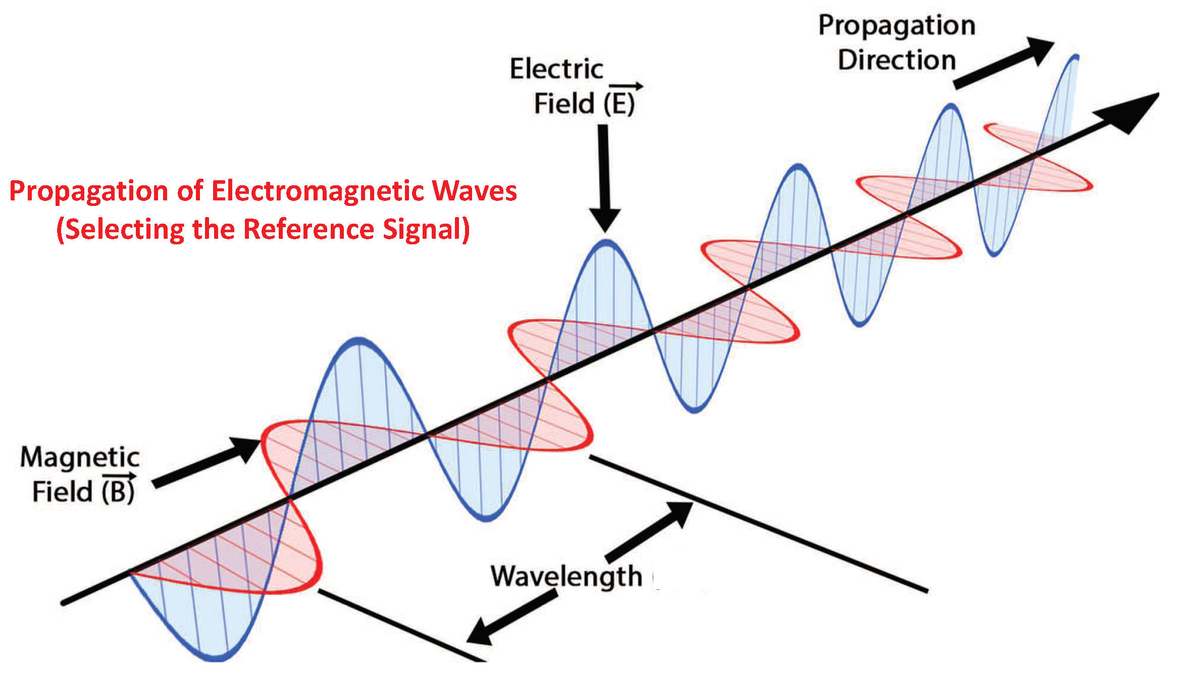
In this section, we incorporate the proposed notion of a cohesive fuzzy set in the application field of filtering the electromagnetic signals for obtaining the reference signal from the number of signals obtained. The propagation and parameter of an electromagnetic signal can be understood through the following diagram given in Figure 2:

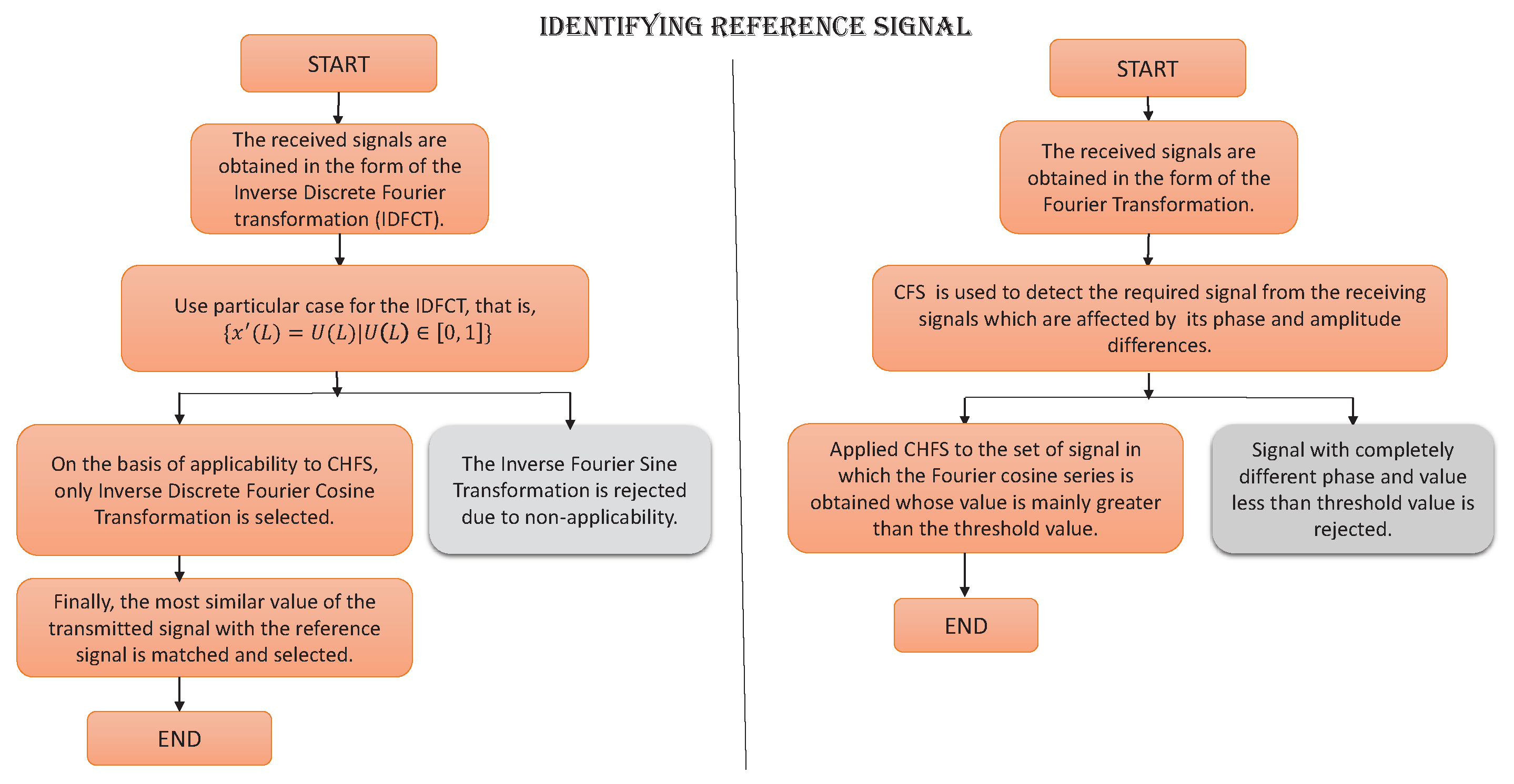
In the subsequent sections, we first present a new methodology by incorporating Fourier Cosine Transformationto identify reference electromagnetic signals and secondly, by using Inverse Discrete Fourier Cosine Transformation, we present another methodology for identifying reference electromagnetic signals. To increase the clarity, the flowchart explaining the procedure is given in Figure 3.

4.1. Identifying Reference Electromagnetic Signal Using Fourier Cosine Transformation(FCT)

Here, the processing of electromagnetic signals was carried over by implementing the introduced concept of a cohesive fuzzy set in identifying the signal of interest among the large number of signals received by the receiver. Ramot et al. [26] demonstrated the use of a complex fuzzy set in signal processing, where L different speech signals and electromagnetic signals, viz., $T_1\left(t\right),T_2\left(t\right),\dots ,T_L\left(t\right)$, have been detected and sampled by the digital receiver. Each received signal is sampled N times. Let $T_l\left(k\right)$ denote the $k^{th}$$\left(1\le k\le N\right)$ sample and the $l^{th}$ signal $\left(1\le l\le L\right)$.

Furthermore, the Fourier transform of the received signals was obtained, and each one is represented as the sum of Fourier components given below:

$$T_l\left(k\right)=\frac{1}{N}\sum _{n=1}^N{C}_{l,n}{e}^{\frac{i2\pi \left(n-1\right)\left(k-1\right)}{N}};$$

(7)

where $C_{l,n}\left(1\le n\le N\right)$ are complex Fourier coefficients of $T_l$.

It may be noted that, in the case of a cohesive fuzzy set, we take the Fourier cosine transform of the received signals, each of which is represented as the sum of Fourier cosine components

$$T_l\left(k\right)=\frac{1}{N}\sum _{n=1}^N{C}_{l,n}cos\left(\frac{i2\pi \left(n-1\right)\left(k-1\right)}{N}\right);$$

(8)

where $C_{l,n}\left(1\le n\le N\right)$ are complex Fourier coefficients of $T_l$.

Therefore, the above-mentioned sum may be rewritten as

$$T_l\left(k\right)=\frac{1}{N}\sum _{n=1}^N{P}_{l,n}{e}^{i{\alpha }_{l,n}}cos\left(\frac{i2\pi \left(n-1\right)\left(k-1\right)}{N}\right);$$

(9)

where $C_{l,n}=A_{l,n}{e}^{i{\alpha }_{l,n}}$, with $P_{l,n}$ and ${\alpha }_{l,n}$ being real-valued, and $P_{l,n}\ge 0$$\forall n$.

The aim of the above-proposed application is to determine whether any signal among received L signals can be identified as the reference signal R. Therefore, in a similar manner, the reference signal R is also sampled N times, and its corresponding Fourier cosine series may be written as

$$R\left(k\right)=\frac{1}{N}\sum _{n=1}^N{P}_{R,n}{e}^{i{\alpha }_{R,n}}cos\left(\frac{i2\pi \left(n-1\right)\left(k-1\right)}{N}\right);$$

(10)

where

$$C_{R,n}=P_{R,n}{e}^{i{\alpha }_{R,n}},with1\le n\le N,$$

$$P_{R,n}and{\alpha }_{R,n}toberealvaluedand{P}_{R,n}\ge 0\forall n.$$

Next, we formally list the steps of the proposed methodology for identifying the reference signal with the help of the similarity measures between the signals $T_1,T_2,\dots ,T_L$ to R as follows:

Step 1: We first normalize the amplitudes of all Fourier cosine coefficients for any candidate signal $T_l\left(1\ne l\ne L\right)$. Suppose $P_l$ denotes the N-dimensional vector of amplitudes of the candidate signal’s $\left(T\right)$ Fourier coefficients:

$$P_l=\left(P_{l,1},P_{l,2},\dots ,P_{l,N}\right),$$

and $P_R$ denotes the N-dimensional vector of amplitudes of the reference signal’s $\left(R\right)$ Fourier coefficients:

$$P_R=\left(P_{R,1},P_{R,2},\dots ,P_{R,N}\right).$$

We consider the normalized vector $Q_l$ in the form given below:

$$Q_l=\frac{1}{P_l.\parallel P_l\parallel },where\parallel P_l\parallel =\sqrt{\sum _{n=1}^N{\left(P_{l,n}\right)}^2},$$

and the normalized vector $Q_R$ in the form given below:

$$Q_R=\frac{1}{P_R.\parallel P_R\parallel },where\parallel P_R\parallel =\sqrt{\sum _{n=1}^N{\left(P_{R,n}\right)}^2}.$$

Thus, the vector $Q_l=(Q_{l,1},Q_{l,2},\dots ,Q_{l,N})$ represents the normalized amplitudes of $T_l^{\prime }s$ Fourier cosine coefficients. Similarly, $Q_R=(Q_{R,1},Q_{R,2},\dots ,Q_{R,N})$ is the normalized amplitude of $R^{\prime }s$ Fourier cosine coefficients.

Step 2: Next, we calculate the complex grade similarity for every Fourier cosine coefficient of $T_l$ in relevance with the reference signal R. Then, the grade of similarity between $C_{l,n}to{C}_{R,n}$ may be denoted by ${\nu }_{R,T_l}\left(n\right)$ and given by

$${\nu }_{R,T_l}\left(n\right)=r_{R,T_l}\left(n\right)e^{i{w}_{R,T_l}\left(n\right)};$$

(11)

where

$$r_{R,T_l}\left(n\right)=e^{\frac{-{\left(Q_{R,n}-Q_{l,n}\right)}^2}{Q_{R,n}{Q}_{l,n}}}and{w}_{R,T_l}=\left({\alpha }_{R,n}-{\alpha }_{l,n}\right).$$

Here, ${\nu }_{R,T_l\left(n\right)}$ represents the complex grade of membership, which includes phase and amplitude terms. The phase term contains the information of the relative phase between the $C_{l,n}$ and $C_{R,n}$. The amplitude term $r_{R,T_l}$ in the range [0, 1] is normalized and used to measure the distance exponentially between the $C_{l,n}$ and $C_{R,n}$. The effect of outside factors such as path loss, the distance of transmission source from the digital receiver, etc., is reduced by using normalized amplitudes $Q_{l,n}$ and $Q_{R,n}$. The case of the relative amplitude of $C_{l,n}$ in $T_l$ is compared with $C_{R,n}$ in R, so that synchronized results may be obtained in either case of strong and weak signals.

Step 3: Furthermore, the complex grade similarity ${\nu }_{R,T_l}$ is obtained by summing the grade similarity of each of the Fourier cosine coefficients ${\nu }_{R,T_l}\left(n\right)\forall n\left(1\le n\le N\right)$, in which either $Q_{l,n}$ or $Q_{R,n}$ must be larger than the $Q_{Threshold}$. This $Q_{Threshold}$ is used to prevent ${\nu }_{R,T_l}$ from the Fourier cosine coefficients with small amplitudes in $T_l$ and R. Next, the sum of the complex grade similarity is divided by the number of coefficients $\left(m\right)$. The considered coefficients of $Q_{l,n}$ and $Q_{R,n}$ must have greater amplitudes compared with the $Q_{Threshold}$ and, consequently, map the amplitude of ${\nu }_{R,T_l}$ in the range of [0, 1] subject to

$${\nu }_{R,T_l}=\frac{{\sum }_M{\nu }_{R,T_l}\left(n\right)}{m};$$

(12)

where

$$M=\left\{n\right|Q_{l,n}or{Q}_{R,n}>Q_{Threshold}\}$$

and the number of elements in $Misdenotedbym.$

Hence, the sum of ${\nu }_{R,T_l}$ given in Equation (12) is totally dependent on the phase term of ${\nu }_{R,T_l}$. The phase term is an important factor to determine whether the grade of similarity increase or decreases among $C_{l,n}^{\prime }s$ and $C_{R,n}^{\prime }s$. This issue of phase has been reduced in our proposed methodology as we are taking Fourier cosine transformation, due to which only one factor will affect the phase term.

Thus, the amplitude of ${\nu }_{R,T_l}$, which is used to determine $T_l$ to R, is subject to the following conditions:

(1)

The identified signal $T_l$ w.r.t R must be close to 1.

(2)

The normalized amplitudes of the Fourier coefficients of $T_l$ and R are similar.

(3)

The relative phases of the Fourier coefficients of candidate and reference signals i.e., $T_l$ and R, are similar.

Step 4: Finally, the electromagnetic signal $T_l$ may be identified as R by comparing the values of $|{\nu }_{\left(R,T_l\right)}|$ to ${\nu }_{Threshold}$. If the obtained value of $|{\nu }_{\left(R,T_l\right)}|$ exceeds the threshold, then the identified signals $T_l$ may be considered as R.

The above-proposed methodology, which utilizes the Fourier Cosine Transformationin calculating the similarity between two signals, is supposed to play a significant role in signal analysis applications, where the relative phase between the Fourier component of the signals is considered to be an important factor.

4.2. Identifying Reference Electromagnetic Signal Using Inverse Discrete Fourier Cosine Transformation(IDFCT)

In this subsection, we use the Inverse Discrete Fourier Cosine Transformationto develop a methodology to find the reference signal among the transmitted signals received by the receiver.

Xueling et al. [63] used the $L^{th}$ Inverse Discrete Fourier Transform (IDFT) coefficient of a length L sequence $x\left(L\right)$ and defined it as

$$x\left(p\right)=\frac{1}{L}\sum _{p=0}^{L-1}{x}^{\prime }\left(L\right)e^{i\frac{2\pi }{L}Lp},p\in 0,1,2,\dots ,L-1;$$

where $x\left(L\right)$ have different values and consider the special case in which $U\left[L\right]=x^{\prime }\left(L\right)$$andU\left[L\right]\in [0,1]$.

In a similar way, we also consider the special case of Inverse Discrete Fourier Cosine Transformation(IDFCT), as shown below:

$$x\left(p\right)=\frac{1}{L}\sum _{p=0}^{L-1}{x}^{\prime }\left(L\right)cos\left(\frac{2\pi }{L}Lp\right),p\in 0,1,2,\dots ,L-1.$$

Definition 13.

The DFCT for $x^{\prime }\left(L\right):1\le L\le L$ is given by matrix in the product form:

$$\left[\begin{array}{c}{x}^{\prime }\left(0\right)\\ x^{\prime }\left(1\right)\\ x^{\prime }\left(2\right)\\ .\\ .\\ .\\ x^{\prime }\left(L-1\right)\end{array}\right]=$$

$$\left[\begin{array}{ccccccc}1& 1& 1& .& .& .& 1\\ 1& cos\left(\frac{-2\pi }{L}\right)& cos\left(\frac{-4\pi }{L}\right)& .& .& .& cos\left(\frac{-2\pi \left(L-1\right)}{L}\right)\\ 1& cos\left(\frac{-4\pi }{L}\right)& cos\left(\frac{-8\pi }{L}\right)& .& .& .& cos\left(\frac{-4\pi \left(L-1\right)}{L}\right)\\ .& .& .& .& .& .& .\\ .& .& .& .& .& .& .\\ .& .& .& .& .& .& .\\ 1& cos\left(\frac{-2\pi \left(L-1\right)}{L}\right)& cos\left(\frac{-4\pi \left(L-1\right)}{L}\right)& .& .& .& cos\left(\frac{-2\pi {\left(L-1\right)}^2}{L}\right)\end{array}\right]$$

$$\left[\begin{array}{c}x\left(0\right)\\ x\left(1\right)\\ x\left(2\right)\\ .\\ .\\ .\\ x\left(L-1\right)\end{array}\right].$$

However, the IDFCT is given by

$$\left[\begin{array}{c}x\left(0\right)\\ x\left(1\right)\\ x\left(2\right)\\ .\\ .\\ .\\ x\left(L-1\right)\end{array}\right]=$$

$$\frac{1}{L}\left[\begin{array}{ccccccc}1& 1& 1& .& .& .& 1\\ 1& cos\left(\frac{2\pi }{L}\right)& cos\left(\frac{4\pi }{L}\right)& .& .& .& cos\left(\frac{2\pi \left(L-1\right)}{L}\right)\\ 1& cos\left(\frac{4\pi }{L}\right)& cos\left(\frac{8\pi }{L}\right)& .& .& .& cos\left(\frac{4\pi \left(L-1\right)}{L}\right)\\ .& .& .& .& .& .& .\\ .& .& .& .& .& .& .\\ .& .& .& .& .& .& .\\ 1& cos\left(\frac{2\pi \left(L-1\right)}{L}\right)& cos\left(\frac{4\pi \left(L-1\right)}{L}\right)& .& .& .& cos\left(\frac{2\pi {\left(L-1\right)}^2}{L}\right)\end{array}\right]$$

$$\left[\begin{array}{c}{x}^{\prime }\left(0\right)\\ x^{\prime }\left(1\right)\\ x^{\prime }\left(2\right)\\ .\\ .\\ .\\ x^{\prime }\left(L-1\right)\end{array}\right].$$

Next, with the help of the above definitions, we propose a new methodology to detect particular signals among the various signals received by the receiver.

Suppose $l(u_1\left(L\right),u_2\left(L\right)u_3\left(L\right),\dots ,u_l\left(L\right))$ is the number of electromagnetic signals received by the receiver, and each of these signals is noted L times. Suppose $x_l\left(L\right)$ is the $l^{th}\left(1\le l\le L\right)$ signal, then the Discrete Fourier Cosine Transformationis given by

$$u_l\left(L\right)=\frac{1}{L}\sum _{p=0}^{L-1}U\left[L\right]cos\left(\frac{2\pi }{L}Lp\right);L,p=0,1,2,\dots ,L-1,$$

(13)

where $U\left[L\right]\in [0,1]$.

Here, $U\left[L\right]={\theta }_S^{\prime }\left(p\right)$ and $\frac{2\pi }{L}Lp=w_S\left(p\right)$ are called the amplitude and phase term, respectively. Thus, Equation (13) denotes the model for signal representation.

Now, we construct a particular kind of matrix to detect the particular signal among the different signals received by the receiver. For this, we consider a reference signal R, which has also been noted L times, and its DFCT is given below:

$$R\left(L\right)=\frac{1}{L}\sum _{p=0}^{L-1}{\theta }^{\prime }\left(p\right)cos\left(\frac{2\pi }{L}Lp\right);L,p=0,1,2,\dots ,L-1,$$

(14)

where ${\theta }^{\prime }\left(p\right)\in [0,1]$.

The procedural steps of the proposed methodology in order to compare the similarity between the two signals are listed as follows:

Step 1:

Expanding $u_l\left(L\right)=\frac{1}{L}{\sum }_{p=0}^{L-1}U\left[L\right]cos\left(\frac{2\pi }{L}Lp\right)$ for $p=0,1,2,\dots ,L-1$ leads to

$$\begin{array}{c}\hfill u_l\left(L\right)=\frac{1}{L}[U\left[0\right]cos\left(\frac{2\pi }{L}L\left(0\right)\right)+U\left[1\right]cos\left(\frac{2\pi }{L}L\left(1\right)\right)+U\left[2\right]\\ \hfill cos\left(\frac{2\pi }{L}L\left(2\right)\right)+\dots +U[L-1]cos\left(\frac{2\pi }{L}L(L-1)\right)].\end{array}$$

(15)

Now, we put the values of $L=0,1,2,\dots ,L-1$ in Equation (15), through which we obtain the $L^{th}$ sample of the signal which is explained by taking individual discrete cases:

For $L=0$ case:

$$\begin{array}{c}\hfill u_l\left(0\right)=\frac{1}{L}[U\left[0\right]cos\left(\frac{2\pi }{L}\left(0\right)\left(0\right)\right)+U\left[1\right]cos\left(\frac{2\pi }{L}\left(0\right)\left(1\right)\right)+U\left[2\right]\\ \hfill cos\left(\frac{2\pi }{L}\left(0\right)\left(2\right)\right)+\dots +U[L-1]cos\left(\frac{2\pi }{L}\left(0\right)(L-1)\right)].\end{array}$$

$$u_l\left(0\right)=\frac{1}{L}\left[U\left[0\right].1+U\left[1\right]1+U\left[2\right].1+\dots +U[L-1].1\right].$$

(16)

For $L=1$ case:

$$\begin{array}{c}\hfill u_l\left(1\right)=\frac{1}{L}[U\left[1\right].1+U\left[1\right]cos\left(\frac{2\pi }{L}\left(1\right)\left(1\right)\right)+U\left[2\right]cos\left(\frac{2\pi }{L}\left(1\right)\left(2\right)\right)\\ \hfill +\dots +U[L-1]sin\left(\frac{2\pi }{L}\left(1\right)(L-1)\right)].\end{array}$$

(17)

For $L=2$ case:

$$\begin{array}{c}\hfill u_l\left(2\right)=\frac{1}{L}[U\left[1\right].1+U\left[1\right]cos\left(\frac{2\pi }{L}\left(2\right)\left(1\right)\right)+U\left[2\right]cos\left(\frac{2\pi }{L}\left(2\right)\left(2\right)\right)+\dots \\ \hfill +U[L-1]cos\left(\frac{2\pi }{L}\left(2\right)(L-1)\right)].\end{array}$$

(18)

Similarly, for $L=L-1$ case:

$$\begin{array}{c}\hfill u_l\left(L-1\right)=\frac{1}{L}[U\left[1\right].1+U\left[1\right]cos\left(\frac{2\pi }{L}(L-1)\left(1\right)\right)+U\left[2\right]\\ \hfill cos\left(\frac{2\pi }{L}(L-1)\left(2\right)\right)+\dots +U[L-1]cos\left(\frac{2\pi }{L}{(L-1)}^2\right)].\end{array}$$

(19)

In a similar manner, we obtain the values for L samples of the reference signal.

Step 2:

Now, we construct the matrix for L-samples of signal $u_l\left(L\right)$ and the reference signal as follows:

$$\left[\begin{array}{c}{u}_l\left(0\right)\\ u_l\left(1\right)\\ u_l\left(2\right)\\ .\\ .\\ .\\ u_l\left(L-1\right)\end{array}\right]=$$

$$\frac{1}{L}\left[\begin{array}{ccccccc}1& 1& 1& .& .& .& 1\\ 1& cos\left(\frac{2\pi }{L}\right)& cos\left(\frac{4\pi }{L}\right)& .& .& .& cos\left(\frac{2\pi \left(L-1\right)}{L}\right)\\ 1& cos\left(\frac{4\pi }{L}\right)& cos\left(\frac{8\pi }{L}\right)& .& .& .& cos\left(\frac{4\pi \left(L-1\right)}{L}\right)\\ .& .& .& .& .& .& .\\ .& .& .& .& .& .& .\\ .& .& .& .& .& .& .\\ 1& cos\left(\frac{2\pi \left(L-1\right)}{L}\right)& cos\left(\frac{4\pi \left(L-1\right)}{L}\right)& .& .& .& cos\left(\frac{2\pi {\left(L-1\right)}^2}{L}\right)\end{array}\right]$$

$$\left[\begin{array}{c}U\left(0\right)\\ U\left(1\right)\\ U\left(2\right)\\ .\\ .\\ .\\ U\left(L-1\right)\end{array}\right]$$

and

$$\left[\begin{array}{c}\theta \left(0\right)\\ \theta \left(1\right)\\ \theta \left(2\right)\\ .\\ .\\ .\\ \theta \left(L-1\right)\end{array}\right]=$$

$$\frac{1}{L}\left[\begin{array}{ccccccc}1& 1& 1& .& .& .& 1\\ 1& cos\left(\frac{2\pi }{L}\right)& cos\left(\frac{4\pi }{L}\right)& .& .& .& cos\left(\frac{2\pi \left(L-1\right)}{L}\right)\\ 1& cos\left(\frac{4\pi }{L}\right)& cos\left(\frac{8\pi }{L}\right)& .& .& .& cos\left(\frac{4\pi \left(L-1\right)}{L}\right)\\ .& .& .& .& .& .& .\\ .& .& .& .& .& .& .\\ .& .& .& .& .& .& .\\ 1& cos\left(\frac{2\pi \left(L-1\right)}{L}\right)& cos\left(\frac{4\pi \left(L-1\right)}{L}\right)& .& .& .& cos\left(\frac{2\pi {\left(L-1\right)}^2}{L}\right)\end{array}\right]$$

$$\left[\begin{array}{c}{\theta }^{\prime }\left(0\right)\\ {\theta }^{\prime }\left(1\right)\\ {\theta }^{\prime }\left(2\right)\\ .\\ .\\ .\\ {\theta }^{\prime }\left(L-1\right)\end{array}\right].$$

It may be noted that the first matrix equation given above represents that the transmitted signal has been obtained by multiplying the phase term matrix and amplitude matrix. Similarly, the second matrix equation given above represents the components of the reference signal.

Step 3:

In view of the above two matrix equations and for the desired analysis, we take the absolute values of all the obtained values to bring them in the range of the disk of radius one in complex plane. These absolute values are given below:

$$\left[\begin{array}{c}|\theta \left(0\right)|\\ |\theta \left(1\right)|\\ |\theta \left(2\right)|\\ .\\ .\\ .\\ |\theta \left(L-1\right)|\end{array}\right]and\left[\begin{array}{c}|u_l\left(0\right)|\\ |u_l\left(1\right)|\\ |u_l\left(2\right)|\\ .\\ .\\ .\\ |u_l\left(L-1\right)|\end{array}\right].$$

Step 4:

Finally, we select the maximum absolute cosine value among all the cases of $u_l\left(l\right)$ and reference signal. Then, the most similar values will be considered to be reference signals.

Example 2.

Suppose that there are four different electromagnetic waves$(u_1\left(L\right),u_2\left(L\right),u_3\left(L\right)$ and $u_4\left(L\right))$which have been detected by the receiver. Then, the sample of each signal is to be taken four times. Assume that $\theta \left(L\right)$ is the reference signal. Then, the Discrete Fourier Cosine Transformation(DFCT) of these signals $u_l\left(L\right)$ and the reference signal $\theta \left(L\right)$ is given by

$$u_l\left(L\right)=\frac{1}{4}\sum _{p=0}^3{U}_l\left[L\right]cos\left(\frac{2\pi }{4}Lp\right);L,p=0,1,2,3;$$

(20)

and

$$\theta \left(L\right)=\frac{1}{4}\sum _{p=0}^3{\theta }^{\prime }\left[L\right]cos\left(\frac{2\pi }{4}Lp\right);L,p=0,1,2,3;$$

(21)

where $U_l\left(L\right),{\theta }^{\prime }\left(L\right)\in [0,1].$ Furthermore, the Equation (20) gives

$$\begin{array}{c}\hfill u_l\left(L\right)=\frac{1}{4}[U\left[0\right]cos\left(\frac{2\pi }{4}L\left(0\right)\right)+U\left[1\right]cos\left(\frac{2\pi }{4}L\left(1\right)\right)+U\left[2\right]\\ \hfill cos\left(\frac{2\pi }{4}L\left(2\right)\right)+U\left[3\right]cos\left(\frac{2\pi }{4}L\left(3\right)\right).\end{array}$$

(22)

Now, we take the values of $L=0,1,2,3$ and subsequently obtain the following equations:

$$\begin{array}{c}\hfill u_l\left(0\right)=\frac{1}{4}[U\left[0\right]cos\left(\frac{2\pi }{4}\left(0\right)\left(0\right)\right)+U\left[1\right]cos\left(\frac{2\pi }{4}\left(0\right)\left(1\right)\right)+U\left[2\right]\\ \hfill cos\left(\frac{2\pi }{4}\left(0\right)\left(2\right)\right)+U\left[3\right]cos\left(\frac{2\pi }{4}\left(0\right)\left(3\right)\right).\end{array}$$

$$u_l\left(0\right)=\frac{1}{4}[U\left[0\right].1+U\left[1\right].1+U\left[2\right].0+U\left[3\right].1.$$

(23)

$$\begin{array}{c}\hfill u_l\left(1\right)=\frac{1}{4}[U\left[0\right]cos\left(\frac{2\pi }{4}\left(1\right)\left(0\right)\right)+U\left[1\right]cos\left(\frac{2\pi }{4}\left(1\right)\left(1\right)\right)+U\left[2\right]\\ \hfill cos\left(\frac{2\pi }{4}\left(1\right)\left(2\right)\right)+U\left[3\right]cos\left(\frac{2\pi }{4}\left(1\right)\left(3\right)\right).\end{array}$$

(24)

$$\begin{array}{c}\hfill u_l\left(2\right)=\frac{1}{4}[U\left[0\right]cos\left(\frac{2\pi }{4}\left(2\right)\left(0\right)\right)+U\left[1\right]cos\left(\frac{2\pi }{4}\left(2\right)\left(1\right)\right)+U\left[2\right]\\ \hfill cos\left(\frac{2\pi }{4}\left(2\right)\left(2\right)\right)+U\left[3\right]cos\left(\frac{2\pi }{4}\left(2\right)\left(3\right)\right).\end{array}$$

(25)

$$\begin{array}{c}\hfill u_l\left(3\right)=\frac{1}{4}[U\left[0\right]cos\left(\frac{2\pi }{4}\left(3\right)\left(0\right)\right)+U\left[1\right]cos\left(\frac{2\pi }{4}\left(3\right)\left(1\right)\right)+U\left[2\right]\\ \hfill cos\left(\frac{2\pi }{4}\left(3\right)\left(2\right)\right)+U\left[3\right]cos\left(\frac{2\pi }{4}\left(3\right)\left(3\right)\right).\end{array}$$

(26)

Next, from all the above Equations (23)–(26), we obtain

$$\left[\begin{array}{c}{u}_l\left(0\right)\\ u_l\left(1\right)\\ u_l\left(2\right)\\ u_l\left(3\right)\end{array}\right]=$$

$$\frac{1}{4}\left[\begin{array}{cccc}1& 1& 1& 1\\ 1& cos\left(\frac{2\pi }{4}\right)& cos\left(\frac{4\pi }{4}\right)& cos\left(\frac{6\pi }{4}\right)\\ 1& cos\left(\frac{4\pi }{4}\right)& cos\left(\frac{8\pi }{4}\right)& cos\left(\frac{12\pi }{4}\right)\\ 1& cos\left(\frac{6\pi }{4}\right)& cos\left(\frac{12\pi }{4}\right)& cos\left(\frac{18\pi }{4}\right)\end{array}\right]\left[\begin{array}{c}{U}_1\left(0\right)\\ U_1\left(1\right)\\ U_1\left(2\right)\\ U_1\left(3\right)\end{array}\right].$$

In a similar manner, for the case of the reference signal, the matrix equation obtained is as follows:

$$\left[\begin{array}{c}\theta \left(0\right)\\ \theta \left(1\right)\\ \theta \left(2\right)\\ \theta \left(3\right)\end{array}\right]=$$

$$\frac{1}{4}\left[\begin{array}{cccc}1& 1& 1& 1\\ 1& cos\left(\frac{2\pi }{4}\right)& cos\left(\frac{4\pi }{4}\right)& cos\left(\frac{6\pi }{4}\right)\\ 1& cos\left(\frac{4\pi }{4}\right)& cos\left(\frac{8\pi }{4}\right)& cos\left(\frac{12\pi }{4}\right)\\ 1& cos\left(\frac{6\pi }{4}\right)& cos\left(\frac{12\pi }{4}\right)& cos\left(\frac{18\pi }{4}\right)\end{array}\right]\left[\begin{array}{c}{\theta }^{\prime }\left(0\right)\\ {\theta }^{\prime }\left(1\right)\\ {\theta }^{\prime }\left(2\right)\\ {\theta }^{\prime }\left(3\right)\end{array}\right].$$

Suppose that the provided values for the reference signal are as below:

$${\theta }^{\prime }\left[p\right]=\left\{\begin{array}{cc}0;\hfill & p=0\hfill \\ 0;\hfill & p=1\hfill \\ 0.2;\hfill & p=2\hfill \\ 1;\hfill & p=3\hfill \end{array}\right.$$

(27)

Then, putting Equation (27) in the above references matrix equation, we obtain

$$\left[\begin{array}{c}\theta \left(0\right)\\ \theta \left(1\right)\\ \theta \left(2\right)\\ \theta \left(3\right)\end{array}\right]=\frac{1}{4}\left[\begin{array}{cccc}1& 1& 1& 1\\ 1& 0& -1& 0\\ 1& -1& 1& -1\\ 1& 0& -1& 0\end{array}\right]\left[\begin{array}{c}0\\ 0\\ 0.2\\ 1\end{array}\right].$$

Now, the absolute value matrix of the reference signal is given as

$$\left[\begin{array}{c}|\theta \left(0\right)|\\ |\theta \left(1\right)|\\ |\theta \left(2\right)|\\ |\theta \left(3\right)|\end{array}\right]=\left[\begin{array}{c}0.3\\ 0.1\\ 0.2\\ 0.1\end{array}\right].$$

The maximum value in the above matrix is 0.3.

Now, for the signal $u_1\left(L\right);L=0,1,2,3$

$$U_1\left[p\right]=\left\{\begin{array}{cc}0.5;\hfill & p=0\hfill \\ 0.7;\hfill & p=1\hfill \\ 0.8;\hfill & p=2\hfill \\ 1;\hfill & p=3\hfill \end{array}\right.$$

(28)

$$\left[\begin{array}{c}{u}_1\left(0\right)\\ u_1\left(1\right)\\ u_1\left(2\right)\\ u_1\left(3\right)\end{array}\right]=\frac{1}{4}\left[\begin{array}{cccc}1& 1& 1& 1\\ 1& 0& -1& 0\\ 1& -1& 1& -1\\ 1& 0& -1& 0\end{array}\right]\left[\begin{array}{c}0.5\\ 0.7\\ 0.8\\ 1\end{array}\right].$$

Now, the absolute value matrix of reference signal $u_1\left(L\right)$ is

$$\left[\begin{array}{c}|u_1\left(0\right)|\\ |u_1\left(1\right)|\\ |u_1\left(2\right)|\\ |u_1\left(3\right)|\end{array}\right]=\left[\begin{array}{c}0.8\\ 0.1\\ 0.1\\ 0.1\end{array}\right].$$

The maximum value in the above matrix is 0.8.

Now, for the signal $u_2\left(L\right);L=0,1,2,3$

$$U_2\left[p\right]=\left\{\begin{array}{cc}0.4;\hfill & p=0\hfill \\ 0.6;\hfill & p=1\hfill \\ 0.8;\hfill & p=2\hfill \\ 1;\hfill & p=3\hfill \end{array}\right.$$

(29)

$$\left[\begin{array}{c}{u}_2\left(0\right)\\ u_2\left(1\right)\\ u_2\left(2\right)\\ u_2\left(3\right)\end{array}\right]=\frac{1}{4}\left[\begin{array}{cccc}1& 1& 1& 1\\ 1& 0& -1& 0\\ 1& -1& 1& -1\\ 1& 0& -1& 0\end{array}\right]\left[\begin{array}{c}0.4\\ 0.6\\ 0.8\\ 1\end{array}\right].$$

Now, the absolute value matrix of reference signal $u_2\left(L\right)$ is

$$\left[\begin{array}{c}|u_2\left(0\right)|\\ |u_2\left(1\right)|\\ |u_2\left(2\right)|\\ |u_2\left(3\right)|\end{array}\right]=\left[\begin{array}{c}0.7\\ 0.1\\ 0.1\\ 0.1\end{array}\right].$$

The maximum value in the above matrix is 0.7.

Now, for the signal $u_3\left(L\right);L=0,1,2,3$

$$U_3\left[p\right]=\left\{\begin{array}{cc}0.6;\hfill & p=0\hfill \\ 1;\hfill & p=1\hfill \\ 0.9;\hfill & p=2\hfill \\ 0.8;\hfill & p=3\hfill \end{array}\right.$$

(30)

$$\left[\begin{array}{c}{u}_3\left(0\right)\\ u_3\left(1\right)\\ u_3\left(2\right)\\ u_3\left(3\right)\end{array}\right]=\frac{1}{4}\left[\begin{array}{cccc}1& 1& 1& 1\\ 1& 0& -1& 0\\ 1& -1& 1& -1\\ 1& 0& -1& 0\end{array}\right]\left[\begin{array}{c}0.6\\ 1\\ 0.9\\ 0.8\end{array}\right].$$

Now, the absolute value matrix of reference signal $u_3\left(L\right)$ is

$$\left[\begin{array}{c}|u_3\left(0\right)|\\ |u_3\left(1\right)|\\ |u_3\left(2\right)|\\ |u_3\left(3\right)|\end{array}\right]=\left[\begin{array}{c}0.8\\ 0.1\\ 0.1\\ 0.1\end{array}\right].$$

The maximum value in the above matrix is 0.8.

Now, for the signal $u_4\left(L\right);L=0,1,2,3$,

$$U_4\left[p\right]=\left\{\begin{array}{cc}0.8;\hfill & p=0\hfill \\ 0.5;\hfill & p=1\hfill \\ 0;\hfill & p=2\hfill \\ 0;\hfill & p=3\hfill \end{array}\right.$$

(31)

$$\left[\begin{array}{c}{u}_4\left(0\right)\\ u_4\left(1\right)\\ u_4\left(2\right)\\ u_4\left(3\right)\end{array}\right]=\frac{1}{4}\left[\begin{array}{cccc}1& 1& 1& 1\\ 1& 0& -1& 0\\ 1& -1& 1& -1\\ 1& 0& -1& 0\end{array}\right]\left[\begin{array}{c}0.8\\ 0.5\\ 0\\ 0\end{array}\right].$$

Now, the absolute value matrix of reference signal $u_4\left(L\right)$ is

$$\left[\begin{array}{c}|u_4\left(0\right)|\\ |u_4\left(1\right)|\\ |u_4\left(2\right)|\\ |u_4\left(3\right)|\end{array}\right]=\left[\begin{array}{c}0.3\\ 0.2\\ 0.3\\ 0.2\end{array}\right].$$

The maximum value in the above matrix is 0.3.

Now, listing all the maximum values and tabulating with the reference value, we obtain

$$\left[\begin{array}{c}\theta \left(L\right)\\ u_1\left(L\right)\\ u_2\left(L\right)\\ u_3\left(L\right)\\ u_4\left(L\right)\end{array}\right]=\left[\begin{array}{c}0.3\\ 0.8\\ 0.7\\ 0.8\\ 0.3\end{array}\right].$$

Based on the above, we determine that the signal $u_4\left(L\right)$ is the reference signal.

5. Cohesive Fuzzy Sets in Solar Activities/Cycles

Planning a space mission requires a good prediction of favorable situations for which a large amount of data related to the solar cycles is required. With the help of estimation based on these data, the best time interval for the space mission may accordingly be predicted. In other words, the conditions of time interval and favorable situations both play a vital role in the success of a particular mission. The most important real-life example is the satellite on Mars (Mangalyaan) which was launched in the year 2013 and was planted in orbit on Mars in the year 2014. In that case, the scientists considered all the possible situations, and the particular time was selected according to the data collected regarding the solar cycles. Thus, we can say that planning under the given set of uncertainties, which may include fuzziness, is an essential component behind the success of any mission.

In this section, we consider the situations which can affect solar activity/cycles and propose a brief outline of the methodology which could effectively help in the planning of such missions related to solar activities in the complex plane. About the above discussions, Yazdanbaksh et al. [64] proposed the concept of an Adaptive Neuro Complex Fuzzy Inferential System (ANCFIS), which played a significant role in the area of solar energy, and also compared the results with the help of two techniques viz. the Adaptive Neuro-Fuzzy Inference System (ANFIS) and Radial Basis Function Networks (RBFNs). In this way, the proposed method and the obtained results were validated.

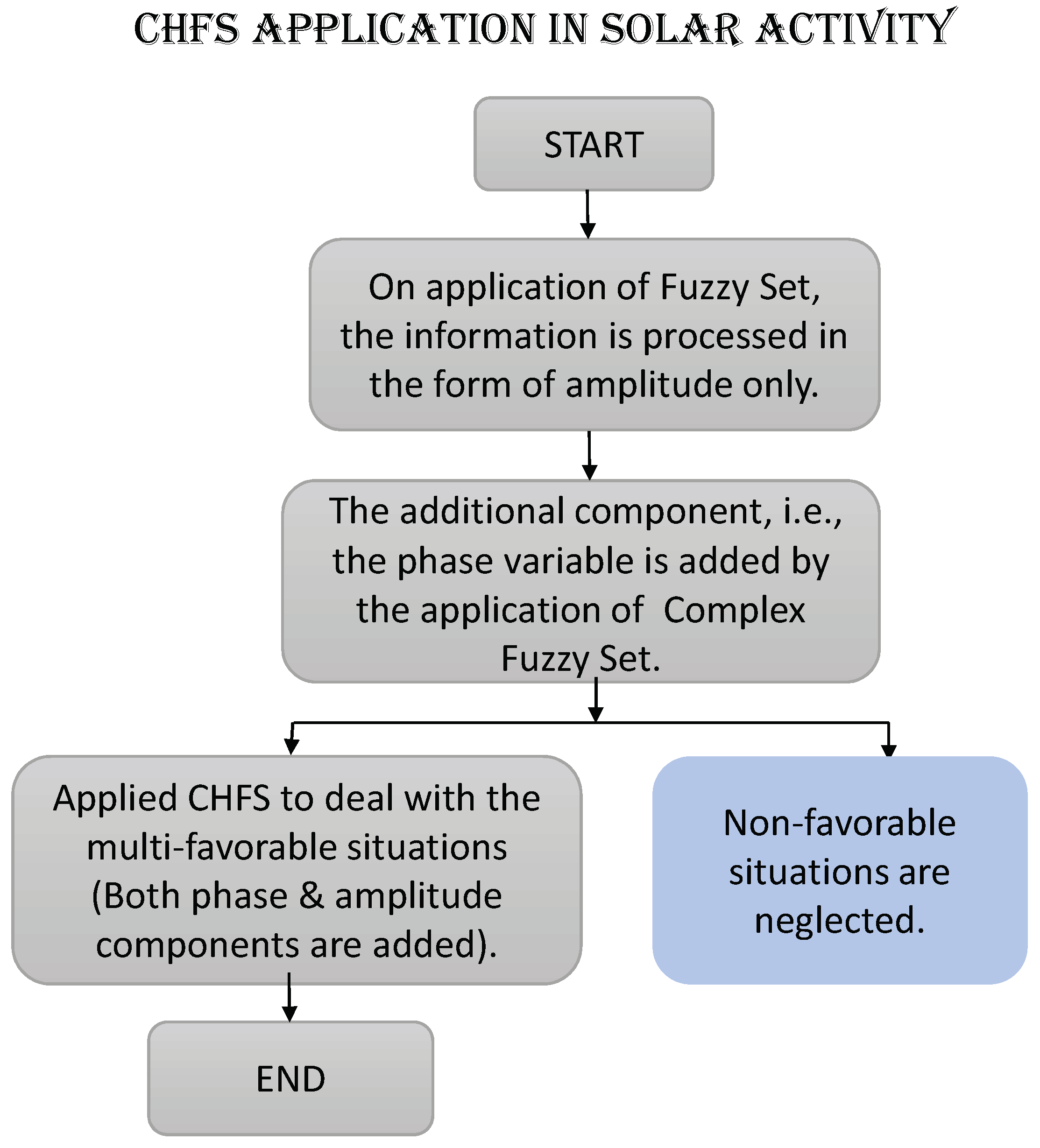
The idea behind implementing the cohesive fuzzy sets in the planning of the solar activities is given by Figure 4 for a better understanding of the concept. Moreover, the important role of CHFS in the case of solar activity is explained with the help of the following example (Example 3).

Example 3.

Every eleven years the sun undergoes a period of activity called the “solar maximum”, followed by a period known as “solar minimum”. During the solar maximum, a large number of sunspots, solar flares, and coronal mass ejections are noticed, which can affect communications and weather on Earth. During the solar minimum, a lesser number of sunspots are observed. This implies that one way of tracking solar activity is by observing the amplitude of sunspots. In this way, the dark blemishes observed on the face of the sun signify the sunspots and the sites where solar flares are observed to occur. As per the data available with the Solar Science resource (NASA) [65], the data collected show the monthly average of the number of sunspots observed since the year 1749. In the case of solar activity, the simple fuzzy set denoted by T is efficient in collecting the data regarding the amplitude of the sunspot, whereas in the case of the complex fuzzy set (CFS), one additional piece of information regarding the phase of the sunspot is obtained. This additional information helps to track the solar cycle with amplitude.

This helps us understand that a complex fuzzy set gives an added advantage over the fuzzy set. In the present work, the proposed notion of a cohesive fuzzy set (CHFS) would certainly have another extra advantage over the complex fuzzy set. It may be noted that when CHFS is used in place of CFS, then in the case of solar activity it encounters the information regarding the interval in which the maximum number of sunspots are obtained. Since the implementation of CHFS will be able to deal with the favorable set of situations in the unit circle on a complex plane, this will therefore not only neglect the useless data, but every element in the favorable set will also be considered.

Now, this is explained in detail with the help of empirical values. Consider an ordinary fuzzy set T with high solar activity, which implies that the set T consists of a large number of sunspots. However, the average number of sunspots observed during the month is used to derive the grade of membership in a particular month. The grade of membership is dependent on the average number of sunspots, i.e., if the number of sunspots is 200, it signifies a large grade of membership, whereas 2 (number of sunspots) is associated with a small grade of membership. If the grade of membership is 0.25 in set T, then it signifies the average number of sunspots in that particular month, say, 50, which can vary considerably if the solar cycle is considered. Therefore, a grade of membership of 0.25 may be treated as inefficient. For example, it has been noted that the maximum number of sunspots in the months of the years 1805 and 1956 was 50, and barely a quarter of the way up, respectively, in the solar cycle. Thus, planning a space mission in these kinds of years was not supposed to be possible. This signifies that it requires long-term planning to execute a mission related to space.

Ramot et al. [26] introduced the notion of the complex fuzzy set, which was able to deal with the phase variable with the explanation of the use of phase in tracking the cycle of solar activity. Furthermore, they explained that the degree of membership can accordingly be increased by using the phase element. Now, the degree of membership depends on both the amplitude and phase variables. The limitation of using CFS is that it only deals with the maximum value of membership of sunspots, whereas the nearby values are sometimes neglected, which can also play an essential role in the tracking of solar activity.

Therefore, to overcome such limitations, it would always be better and advantageous to apply the proposed notion of a cohesive fuzzy set (CHFS), which deals with the set of favorable values which not only counter the limitation of the ordinary fuzzy set but also provide an added feature over CFS. Hence, we can assert that CHFS plays a very important role in the planning of any solar activity. It is important to consider the following three conditions for achieving favorable sets in planning a solar activity:

• In the first condition, the amplitude will be in the range of [0.5, 1], and no restriction is applied to the phase element.
• Secondly, the phase element will be in the range of $\left[\frac{\pi }{2},\frac{3\pi }{2}\right]$, and no restriction is applied on the amplitude.
• Thirdly, the amplitude and phase element will always lie in the range [0.5, 1] and $\left[\frac{\pi }{2},\frac{3\pi }{2}\right]$, respectively.

It may be noted that all the above conditions can always be better dealt with using the help of cohesive fuzzy sets. Now, the first condition is only applicable for the year in which the average number of sunspots is between 100 to 200, which will lead to a grade of membership between [0.5, 1]. This will automatically increase the grade of membership irrespective of the membership of phase, likely from the year 1990–1994 (according to the data given in ref. [65]). Such conditions will automatically neglect the unfavorable data for any solar activity.

In the second case, we restrict the phase parameter and select the years in which the average number of sunspots is much less (such as in the year 1995—according to ref. [65]). In those years, due to the decrease in the average number of sunspots, the degree of membership will also decrease. Therefore, to increase the membership degree, it is advisable to increase the phase element. In this way, in the years when there is less amplitude of sunspots, a space mission can also be planned.

In the third case, this condition relates to the set of the most favorable situations in which we restrict both amplitude and phase terms in the intervals in which both are increasing. Hence, the degree of membership in this set will be the maximum for almost all the data. Thus, planning a space mission in this interval of years will increase the chances of success. In this manner, all the nearby situations cannot be neglected, and each of the elements of the sets in all the above cases can be dealt with using the help of CHFS. The cases explained above can accordingly be worked out depending on the place of the experiment. Therefore, the researchers must collect the data related to the solar cycles according to the places and then plan any solar activity.

6. Comparative Analysis and Advantages of the Proposed Methodology

The advantages of CHFS in contrast with the utilization of fuzzy sets and complex fuzzy sets are explained with the help of a characteristic table given as

Table 1. Characteristic comparison with the existing sets.

Degree of Membership	FS	CFS	HFS	CHFS
Amplitude	✓	✓	✓	✓
Phase	×	✓	×	✓
Advantages	Degree of membership in case of amplitude is obtained.	Degree of membership in case of amplitude and phase is obtained.	Degree of membership in case of favorable situation is obtained.	Degree of membership in case of amplitude and phase is obtained.
Advantages over other	It is not able to track the solar cycle.	It contains both the useful data as well as the nonuseful data, which consumes time. Secondly, it also misses some of the useful data, as only the max value is considered.	It contains favorable data but in the range [0, 1].	It only contains the favorable values in the set, and also all the values are considered.

.

• The advantage of CHFS is that it contains the properties of both complex fuzzy set (CFS) and hesitant fuzzy set (HFS), which enhances the efficiency of the proposed set in solving the problems more efficiently.
• The CHFS contains the ability to address the problems of time periodicity and handling the two-dimensional data set, which could not be addressed by Type-2 fuzzy sets or some other extensions of fuzzy sets. Moreover, it deals with the set of favorable values, which not only counter the limitation of the ordinary fuzzy set but also provide an added feature over CFS.
• The proposed notion of CHFS deals with the favorable set, i.e., in the case of signals, a favorable set of Cosine Transformation is considered, but the Sine Transformation is rejected due to the limitation of the problem under consideration. This limitation of the proposed methodology may be resolved in the future by introducing some new concepts with some other examples.
• Similarly, in the case of solar cycles, the different particular favorable cases were selected based on the structure of the problem.

7. Conclusions and Scope for Future Work

The new extension set coined as a cohesive fuzzy set has been successfully proposed, which has the dual benefits of the complex fuzzy set with coverage of the hesitant fuzzy set. We studied the various operations and several useful identities of the CHFS, which duly explained the process of selection of the best alternative among the available multifavorable situations with the possibility of its range in the extended unit circle of the complex plane. We successfully established the relationship between the cohesive fuzzy set and complex intuitionistic fuzzy set and also validated the obtained results. The identification process of the reference signal among various transmitted electromagnetic signals was accomplished by utilizing the feature of cohesive fuzzy set and Fourier cosine transform/inverse Fourier cosine transform. Moreover, the process of identifying the maximum number of sunspots in a particular interval under a solar activity has been discussed and explained with suitable references. The advantageous features of the proposed methodology are tabulated for better readability. The proposed notion of a cohesive fuzzy set appears to be a promising one for addressing certain real-life situations which cannot be dealt with by complex fuzzy set and other extensions of fuzzy sets. The concepts of aggregation operators and complex hesitant fuzzy relations for CHFS can further be worked out for solving various types of decision-making problems. In addition to this, some new similarity measures in the complex domain may be introduced and utilized for the problems of pattern recognition and medical diagnosis.