
A New Adaptive Accelerated Levenberg–Marquardt Method for Solving Nonlinear Equations and Its Applications in Supply Chain Problems

1
School of Mathematics and Statistics, Beihua University, Jilin 132013, China
2
School of Information Engineering, Hainan Vocational University of Science and Technology, Hainan 571126, China
*
Author to whom correspondence should be addressed.
Symmetry 2023, 15(3), 588; https://doi.org/10.3390/sym15030588
Submission received: 10 February 2023
/
Revised: 21 February 2023
/
Accepted: 22 February 2023
/
Published: 24 February 2023
(This article belongs to the Topic Evolutionary Differential Equations, Dynamic Systems, Computation and Optimization)
Abstract
:In this paper, a new adaptive Levenberg–Marquardt method is proposed to solve the nonlinear equations including supply chain optimization problems. We present a new adaptive update rule which is a segmented function on the ratio between the actual and predicted reductions of the objective function to accept a large number of unsuccessful iterations and avoid jumping in local areas. The global convergence and quadratic convergence of the proposed method are proved by using the trust region technique and local error bound condition, respectively. In addition, we use the proposed algorithm to test on the symmetric and asymmetric linear equations. Numerical results show that the proposed method has good numerical performance and development prospects. Furthermore, we apply the algorithm to solve the fresh agricultural products supply chain optimization problems.
1. Introduction
With the development of science and technology, more and more fields are involved in the solution of nonlinear equation problems, such as chemistry, mechanics, economics and product management [1,2,3,4]. For example, decentralized decision models in supply chain management and gas pressure volume models in physics can be converted into the following nonlinear equations
where is a continuously differentiable function. In particular, symmetric nonlinear equations with the Jacobian matrix symmetry also have a wide range of applications, such as the gradient mapping of unconstrained optimization problem, the Karush–Kuhn–Tucker (KKT) of equality constrained optimization problem, and other fields [5,6].
The steepest descent method, Newton method, quasi-Newton method, Gauss–Newton (GN) method are commonly used iterative methods for solving (1) [7,8,9,10]. The GN method is one of the most famous methods, when the Jacobian matrix is Lipschitz continuous and nonsingular at the solution of (1), the GN method has quadratic convergence. However, when the Jacobian matrix is singular or nearly singular, the GN method may not be well defined. In order to overcome this difficulty, the Levenberg–Marquardt (LM) method [11,12] for solving (1) was proposed. At the k-th iteration, the trial step is
where , is a Jacobian matrix of at , which may be a symmetric matrix or non-symmetric matrix, I is an identity matrix and the LM parameter .
The LM method ensures the uniqueness of solution of (1), and it also has quadratic convergence if is Lipschitz continuous, nonsingular at the solution, and is selected appropriately. In this sense, the update of the LM parameter has a great impact on the performance and efficiency of algorithm, many effective LM parameters have been proposed. Yamashita and Fukushima [13] chose the LM parameter as , and proved that the LM method had quadratic convergence under the local error bound condition and is Lipschitz continuous at the solution. However, when is far away from the solution set, may be very large, which makes very small and reduces the efficiency of algorithm; when is sufficiently close to the solution set, may be smaller than the machine epsilon and lose its role.
Based on these observations, Fan and Yuan [14] generalized the LM parameter in [13], and proved that the numerical results for choosing is better than choosing . Fan [15] first introduced the regularization factor into the LM method and chose , with numerical results showing that this choice of provides the best performance. However, when is far away from the solution set, the choice of both LM parameters does not provide good results. Therefore, to avoid this situation, Fan and Pan [16] chose the LM parameter as , in which is updated by a trust region technique. They defined as a positive function of , i.e.,
where . This update strategy can obtain larger LM trial steps, so that the iterative sequence can quickly converge to the solution set when is far away from the solution set. Amini et al. [17] chose the LM parameter as
It is clear that when is far away from the solution set and is very large, is close to 1, so is close to . The choice of speeds up the efficiency of the algorithm more than previous LM parameters.
In addition to the above different choices of LM parameters, the introduction of adaptive technology also has a great impact on the LM method. As we all know, the ratio between the actual and predicted reductions of the objective function reflects the degree to which the approximate quadratic model approaches the value function. To make more use of information about the ratio, Fan and Yuan [18] proposed an adaptive LM method by selecting , , is a continuous non-negative function about , and . The introduction of avoids discontinuities when crossing the threshold of the ratio, and better numerical results can be obtained.
In fact, similar adaptive techniques have been proposed in the trust region algorithms. If is sufficiently greater than 1, the iteration is too successful at this time, then we can reduce to a very small value. Then, the algorithm will continue to perform a large number of consecutive unsuccessful iterations. On the other hand, if , is a far-from-satisfactory trial step, then we can increase greatly. At this moment, the successive iteration points will be close to each other and the algorithm will converge slowly. Therefore, Hei [19] proposed an R-function by using an adaptive update strategy to update the trust region radius , i.e., . Furthermore, Walmag and Delhez [20] proposed a -function to update the trust region radius, i.e., , where is a non-negative and bounded function about . On this basis, Lu et al. [21] argued that the consistency between the model and the objective function is not good enough in too-successful iterations, so an L-function was proposed to update the trust region radius. They showed that the L-function contains some favorable features of the R-function and the -function, and the method is more efficient in too-successful iterations. In this paper, we want to learn from the presentation of the L-function and provide a new adaptive strategy to update the LM parameter. Our innovations mainly include the following:
◊ A new adaptive accelerated LM method is proposed, which can improve the consistency between the model and the objective function in too-successful iterations by using the ratio information of the actual reduction to the predicted reduction;
◊ The new algorithm can solve the situation in which the iterative sequence is far away from the optimal solution set, accept a large number of unsuccessful iterations and avoid jumping in local areas, thus improving the efficiency and stability of the algorithm;
◊ The new adaptive accelerated LM method has global convergence and quadratic convergence under local error bound.
The rest of this paper is organized as follows. In Section 2, we describe in detail a new adaptive accelerated LM method which makes full use of the ratio information. Furthermore, we demonstrate that the new algorithm has global convergence under the appropriate conditions and maintains quadratic convergence under local error bound condition. In Section 3, numerical results are given, indicating that the new algorithm is efficient. The conclusion is given in the last section.
2. Methodology
2.1. The Adaptive Accelerated Levenberg–Marquardt Method
In this section, our main aim is to discuss how to update the LM parameter to propose a new adaptive accelerated LM method. It is easy to see from (2) that is the solution to the optimization problem
If
then is also the solution of the subproblem
Therefore, the LM method can be regarded as a trust region method, which implicitly modifies the trust region radius . The difference between the general trust region method and the LM method is that the LM method does not directly update the trust region radius, but updates the regularization factor .
We define the actual reduction and predicted reduction of the merit function at the k-th iteration as
and
The ratio between the actual and predicted reductions of the objective function is defined by
This ratio determines whether the trial step is accepted. Here, we choose the LM parameter as
The usual empirical rules [22,23,24,25] of can be usually summarized as follows
where and are constants.
Iterations with greater than are very successful iterations. In this case, it is usually assumed that the approximation of the model function to the objective function is accurate and should be reduced. However, at too-successful iterations, i.e., is sufficiently greater than 1, the consistency between the model and the objective function is not good enough. Thus, we use an adaptive strategy to update the factor , i.e., , where is a function about .
We construct as follows:
where and are constants. Here, satisfies the following properties
If we obtain a satisfactory trial step and ratio , then we accept trial step and reduce ; otherwise, we reject trial step and increase . At too-successful iterations, the actual reduction of the objective function obtained at iteration k is obviously greater than the predicted reduction. Although the current iteration allows the algorithm to progress towards the optimum, the approximation of the model function to the objective function is bad. Therefore, to avoid reducing too quickly, we use the K-function to update .
According to the properties of the K-function, the rate of reduction is the fastest when is close to 1, i.e., when the model function provides an accurate local approximation of the objective function. The new idea we propose is to allow to be updated at a variable rate according to , which would improve the efficiency and stability of the algorithm.
Based on the above analysis, we state a description of the new adaptive accelerated LM method (Algorithm 1) as follows.
In Algorithm 1, m is a given lower bound of the parameter . It is introduced to prevent the step from being too large when the sequence is near the solution.
| Algorithm 1 NAALM. |
2.2. The Global Convergence
In this section, to obtain the global convergence of NAALM algorithm, we make the following assumption.
Assumption 1.
is continuously differentiable, and the Jacobian matrix are Lipschitz continuous, i.e., there exist positive constants and such that
and
Lemma 1.
Let be computed by (12), then the inequality
holds for all .
Proof.
The proof is complete. □
Theorem 1.
Under the conditions of Assumption 1, the sequence generated by NAALM algorithm satisfies
Proof.
If the theorem is not true, then there exist a positive and infinitely many k such that
Let , be the sets of all indices that satisfy
and
Then, is an infinite set. In the following, we will derive the contradictions regarding whether is finite or infinite.
Case (I) is finite.
It follows from the definition of that the set
is also finite. Let be the largest index of . Then, we know that holds for all . Define the indices set
Suppose . It is easy to see that . Moreover, we have . Otherwise, if , then , which contradicts the fact that is the largest index of . Hence, we have . By induction, we know that and hold for all .
It now follows from Step 3 of the NAALM Algorithm that for all , which imply
due to (12)–(14) and for all . Hence, we have
Furthermore, it follows from (21), (23) and Lemma 1 that
that is, . In view of the updating rule of , we know that there exists a positive constant such that holds for all sufficiently large k, which is a contradiction to (22). Hence, the supposition (21) cannot be true while is finite.
Case (II) is infinite.
It follows from Lemma 1 that
which gives
Relation (27) and the fact that (21) holds for infinitely many k indicate that there exists a with such that
By induction, we obtain that for all . This result and (26) mean that
2.3. Local Convergence
In this section, we will study the local convergence properties of the NAALM algorithm by using the singular value decomposition (SVD) technique. We assume that the sequence generated by the NAALM algorithm converges to the nonempty solution set and lies in some neighborhood of . Firstly, we present some assumptions which the local convergence theory required.
Definition 1.
Let such that , we say that provides a local error bound on for (1) if there exists a positive constant such that
where is the distance from x to .
Assumption 2.
(i) is continuously differentiable, and is Lipschitz continuous on with , i.e., there exists a positive constant such that
(ii) provides a local error bound on some neighborhood of , i.e., there exists a positive constant such that
By the Lipschitzness of the Jacobian matrix proposed by (30), we have
and
where is a positive constant.
In the following, we use to denote the vector in that satisfies
To obtain the local convergence rate of , we present some lemmas.
Lemma 2.
Under the conditions of Assumption 2, for all sufficiently large k, there exists a constant such that
Proof.
Lemma 3.
Under the conditions of Assumption 2, for all sufficiently large k, there exists a positive constant such that
Proof.
First, we show that for sufficiently large k, the following inequality holds
We consider two cases. In one case, if , then the definition of and Assumption 2 imply that
In the other case, if , then we have
Inequalities (41) and (42), together with Lemma 2 show that
which gives (40). Hence, it follows from (40), Assumption 2 and Lemma 2 that
Therefore, we have , thus, there exists a constant such that for all large k. The proof is completed. □
Without generality, we assume rank for all . Suppose the SVD of is
where with and , are orthogonal matrices. Correspondingly, we consider SVD of by
where , are orthogonal matrixes, with and with .
Lemma 4.
Under the conditions of Assumption 2, for all sufficiently large k, we have
;
;
;
.
Proof.
The result follows immediately from (16). By (15) and the theory of matrix perturbation [26], we have
which implies that
Let , where is the pseudo-inverse of . It is easy to see that is the least-squares solution of , so we obtain from (32) that
Let and . Since is the least-squares solution of , it follows from (32) that
Due to the orthogonality of and , we obtain the result .
Since converges to the solution set , we assume that holds for all sufficiently large k. Then, it follows from (46) that
It then follows from Lemmas 3 and 4 that
The proof is completed. □
We can state the quadratic convergence result of the NAALM algorithm.
Theorem 2.
Let the sequence be generated by the NAALM algorithm, under Assumption 2, the sequence converges quadratically to a solution of nonlinear Equation (1).
Proof.
It follows from Assumption 2, Lemma 2 and (47) that
On the other hand, it is clear that
It follows from Lemma 2 that, for any sufficiently large k, we have
Therefore, . This, along with (48), indicates that
which implies that is quadratically convergent to a solution of set . The proof is completed. □
3. Numerical Results
In this section, the numerical performance of NAALM algorithm will be listed. All codes were written in MATLAB R2016b on a PC with 1.19 GHz, 8.00 GB RAM, using Windows 11 operation system. In this section, we will expand on the following two aspects. On the one hand, the effectiveness of the NAALM algorithm is illustrated by comparing it with other algorithms on some test questions. On the other hand, it shows that the NAALM algorithm has good development prospects by applying the algorithm to a fresh agricultural products supply chain problem.
3.1. Some Singular Nonlinear Equations Problems
The test problems are constructed by modifying the nonsingular problems given by Moré et al. [27], which have the following form as [28]:
where is the standard test function, has full column rank with and x is a solution of the equation . According to the definition of , we obtain
where is Jacobian matrix of at with rank and . In our test problems, some of are symmetric matrices and some are non-symmetric matrices. Note that some roots of may not be roots of . Similar to [28], we construct two sets of singular problems while have rank or , by choosing
and
We test our NAALM algorithm on some singular nonlinear equations, and compare it with the self-adaptive Levenberg–Marquardt algorithm (SLM) proposed in [18]. The main differences between these two algorithms are in the updating rule of .
We set , , , , , , , , for all the tests. All test methods are terminated when . The algorithm is considered to fail when the number of iterations exceeds 500. Considering the global convergence of the algorithms, we run each test problem for five starting points, , , , and , where is given by [28]. For n as a variable, we take , , respectively.
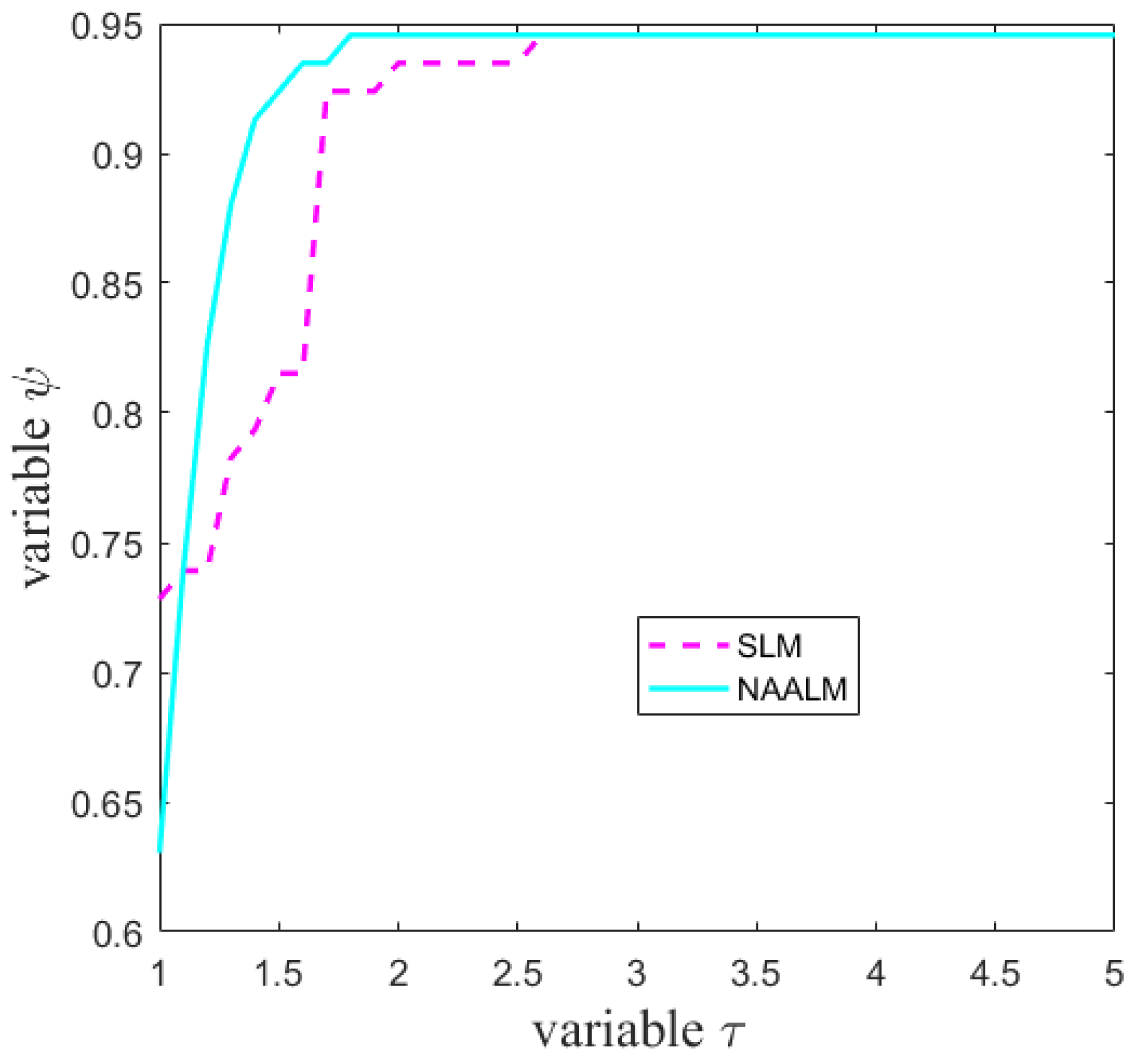
The performance profile of two algorithms. including the number of iterations (NI), function evaluations (NF), gradient evaluations (NG) and CPU time (CPU), is analyzed using the profiles of Dolan and Mor [29]. Let Y and W be the set of methods and test problems, , be the number of methods and test problems, respectively. The performance profile is for each and defined that is NI or NF or NG or CPU required to solve problems w by method y. Furthermore, the performance profile is obtained by
where , is the number of the elements in a set, and is the performance ratio defined as
Generally, the method whose performance profile plot is on the top right will represent the best method.
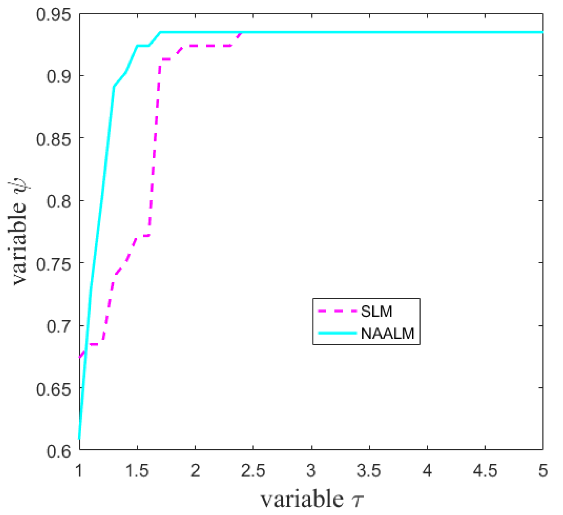
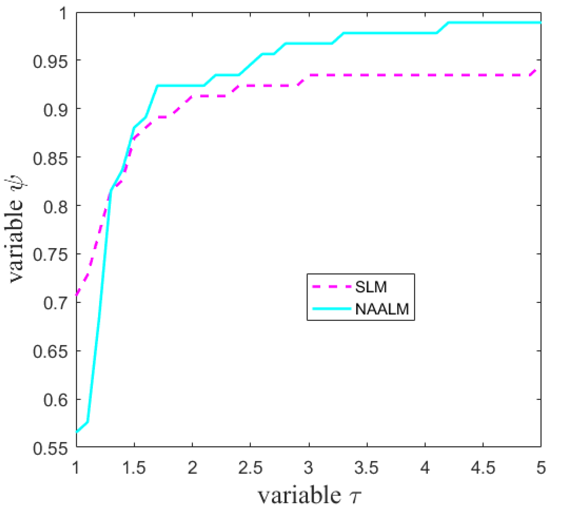
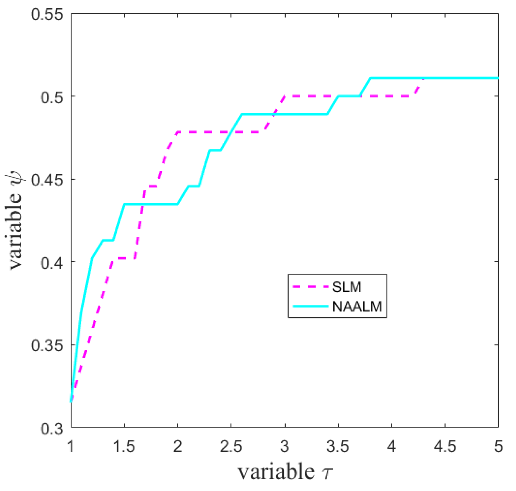
As can be seen from Figure 1, the NAALM algorithm is better than the SLM algorithm in terms of the number of iterations, especially when , the curve of NAALM algorithm becomes stable, which indicates that NAALM algorithm can solve the problem only with fewer iterations. In terms of function evaluations, as shown in Figure 2, the NAALM algorithm curve in , it has reached a stable state, while SLM algorithm can reach a stable state only when the curve coincides with that of NAALM algorithm at ; Figure 3 shows the performance diagram of the SLM algorithm and the NAALM algorithm in the Jacobian matrix. It can be seen that the NAALM algorithm can successfully solve test problems up to 98%, while SLM can only reach 94%, which shows that the NAALM algorithm can reduce the calculation times of the Jacobian matrix and save the calculation amount. Figure 4 shows the CPU time performance of the NAALM algorithm and the SLM algorithm. It can be seen from the figure that when , the curves of the NAALM algorithm and the SLM algorithm are similar, but when , both the NAALM algorithm and the SLM algorithm tend to be stable and coincide. Therefore, Figure 1, Figure 2, Figure 3 and Figure 4 show that the accelerated version of the LM algorithm proposed in this paper can not only converge to the solution quickly, but also reduce the computation amount of the Jacobian matrix.
3.2. Supply Chain Optimization Problems
The security and stability of the supply chain has a great impact on promoting high-quality and sustainable development of the economy. Therefore, supply chain has been applied to many fields, such as low-carbon supply chain, manufacturing green supply chain, food trade supply chain. In recent years, with the improvement of living standards, the quality of fresh agricultural products has attracted widespread attention from consumers. In order to meet the demand of consumers for high quality and low price of fresh agricultural products, we use the NAALM algorithm to study how suppliers and retailers make decisions to maximize both their own profits and the total profit of the fresh agricultural products supply chain under the decentralized policy.
In this supply chain, as the leader of Stackelberg game, fresh agricultural product suppliers supply the same variety of ordinary fresh agricultural products (ofp) and green fresh agricultural products (gfp) to retailers as followers, while retailers sell them to consumers. Suppliers need to choose the optimal wholesale price strategy of two fresh agricultural products, and retailers need to choose the optimal retail price strategy of two fresh agricultural products and determine the order quantity of two fresh agricultural products by market demand.
Without considering the impact of emergencies, the market demand for fresh agricultural products is relatively stable, and it is only related to price and freshness. Due to the substitution of the same varieties of ofp and gfp, there is a competitive relationship in the demand market. Based on the demand function theory of alternative price competition, it is assumed that the demand function of two fresh agricultural products is as follows
where , represent the market demand of gfp and ofp, respectively, a represents the total potential market capacity of fresh agricultural products, , represent the retail price of gfp and ofp, respectively, b is the price sensitivity coefficient, r is the competitive substitution coefficient of the two products, and it satisfies , is the freshness of fresh produce when it arrives at the retailer’s store.
Under the decentralized policy, we regard suppliers and retailers as independent entities, and both with the goal of maximizing their respective interests. Now, the profit function of fresh agricultural products retailer is as follows
where , represent the supply price of gfp and ofp, respectively, and the profit function of fresh agricultural products suppliers is as follows
where represents the quantity loss of fresh produce when it reaches the retailer’s store, , represents the unit production cost of gfp and ofp, respectively. Obviously, and . We record the total profit of fresh agricultural products supply chain as follows:
With reference to the setting of the parameters in the relevant literature [30], we set: , , , , , , . These values satisfy the theoretical proof in [30] and can guarantee that the optimal value has practical significance. Now, we transform the unconstrained optimization problem (51) into a nonlinear equation problem, and then choose different initial points and use the NAALM algorithm to solve the nonlinear equation problem.
As can be seen from Table 1, with certain parameters, the NAALM algorithm can be used to solve the optimization problem, so as to obtain the optimal pricing strategy with maximum profit in the supply chain led by suppliers under the decentralized policy. In addition, the global convergence and robustness of the NAALM algorithm are verified according to different initial values and the number of iterations.
4. Conclusions
We constructed a new function that makes full use of the ratio information to update LM parameters adaptively. Based on this new LM parameter, we presented an adaptive accelerated Levenberg–Marquardt method for solving nonlinear equations. Furthermore, we showed the global convergence analysis of the proposed algorithm. Furthermore, the quadratic convergence is also obtained under the local error bound condition. Numerical experiments demonstrated that our method has good numerical performance. In addition, the application of the NAALM algorithm to a supply chain problem showed that the new algorithm has a good application prospect. We further highlight that the proposed NAALM algorithm can be used in other fields, such as the symmetric system of nonlinear equations. It is vital to note that the method’s convergence analysis in Hölderian local error bound condition will be taken into account in our future work.
Author Contributions
Conceptualization, R.L., M.C. and G.Z.; methodology, R.L., M.C. and G.Z.; software, R.L., M.C. and G.Z. validation, R.L., M.C. and G.Z.; formal analysis, R.L., M.C. and G.Z.; investigation, R.L., M.C. and G.Z.; resources, R.L., M.C. and G.Z.; data curation, R.L., M.C. and G.Z.; writing—original draft preparation, R.L., M.C. and G.Z.; writing—review and editing, R.L., M.C. and G.Z. All authors have read and agreed to the published version of the manuscript.
Funding
This work is supported by the key project of natural science foundation joint fund of Jilin Province (YDZJ202101ZYTS167, YDZJ202201ZYTS303); the project of education department of Jilin Province (JJKH20210030KJ, JJKH20230054KJ); the graduate innovation project of Beihua University (2022033, 2021002); the youth science and technology innovation team cultivation program of Beihua University.
Data Availability Statement
Not applicable.
Acknowledgments
The authors would like to thank the anonymous referees and editor for reading this paper carefully, providing valuable suggestions and comments, which grately improved the final version.
Conflicts of Interest
The authors declare no conflict of interest.
References
- Musa, Y.B.; Waziri, M.Y.; Noor, M.A. An efficient method for solving system for nonlinear equation. J. Math. Anal. 2022, 13, 1–10. [Google Scholar]
- Ribeiro, S.; Lopes, L.G. Overview and computational analysis of PSO variants for solving systems of nonlinear equations. Commun. Intell. Syst. 2022, 461, 1093–1105. [Google Scholar]
- Ji, J.Y.; Wong, M.L. Decomposition-based multiobjective optimization for nonlinear equation systems with many and infinitely many roots. Inf. Sci. 2022, 610, 605–623. [Google Scholar] [CrossRef]
- Artacho, F.J.A.; Fleming, R.; Vuong, P.T. Accelerating the DC algorithm for smooth functions. Math. Program. 2018, 169B, 95–118. [Google Scholar] [CrossRef] [Green Version]
- Sabi’u, J.; Muangchoo, K.; Shah, A.; Abubakar, A.B.; Aremu, K.O. An inexact optimal hybrid conjugate gradient method for solving symmetric nonlinear equations. Symmetry 2021, 13, 1829. [Google Scholar] [CrossRef]
- Sabi’u, J.; Muangchoo, K.; Shah, A.; Abubakar, A.B.; Jolaoso, L.O. A modified PRP-CG type derivative-free algorithm with optimal choices for solving large-scale nonlinear symmetric equations. Symmetry 2021, 13, 234. [Google Scholar] [CrossRef]
- Niri, T.D.; Heydari, M.; Hosseini, M.M. Correction of trust region method with a new modified Newton method. Int. J. Comput. Math. 2022, 97, 1–15. [Google Scholar]
- Bellavia, S.; Morini, B.; Rebegoldi, S. On the convergence properties of a stochastic trust-region method with inexact restoration. Axioms 2023, 12, 38. [Google Scholar] [CrossRef]
- Zheng, L.; Chen, L.; Ma, Y.F. A variant of the Levenberg-Marquardt method with adaptive parameters for systems of nonlinear equations. AIMS Math. 2021, 7, 1241–1256. [Google Scholar] [CrossRef]
- Yudin, N.E. Adaptive Gauss-Newton method for solving systems of nonlinear equations. Dokl. Math. 2021, 104, 293–296. [Google Scholar] [CrossRef]
- Levenberg, K. A method for the solution of certain nonlinear problems in least squares. Quart. Appl. Math. 1944, 2, 164–166. [Google Scholar] [CrossRef] [Green Version]
- Marquardt, D.W. An algorithm for least-squares estimation of nonlinear inequalities. SIAM J. Appl. Math. 1963, 11, 431–441. [Google Scholar] [CrossRef]
- Yamashita, N.; Fukushima, M. On the Rate of Convergence of the Levenberg-Marquardt Method. Computing 2001, 15, 239–249. [Google Scholar]
- Fan, J.Y.; Yuan, Y.X. On the Convergence of a New Levenberg-Marquardt Method; Report No. 005, AMSS; Chinese Academy of Sciences: Beijing, China, 2001. [Google Scholar]
- Fan, J.Y. A modified Levenberg-Marquardt algorithm for singular system of nonlinear equation. J. Comput. Math. 2003, 21, 625–636. [Google Scholar]
- Fan, J.Y.; Pan, J.Y. A note on the Levenberg-Marquardt parameter. Appl. Mathe. Comput. 2009, 207, 351–359. [Google Scholar] [CrossRef]
- Amini, K.; Rostami, F.; Caristi, G. An efficient Levenberg-Marquardt method with a new LM parameter for systems of nonlinear equations. Optimization 2018, 67, 637–650. [Google Scholar] [CrossRef]
- Fan, J.Y.; Yuan, Y.X. Convergence properties of a self-adaptive Levenberg-Marquardt algorithm under local error bound condition. Comput. Optim. Appl. 2006, 34, 47–62. [Google Scholar] [CrossRef]
- Hei, L. A self-adaptive trust region algorithm. J. Comput. Math. 2003, 21, 229–236. [Google Scholar]
- Walmag, J.M.B.; Delhez, E.J.M. A note on trust-region radius update. Siam J. Optim. 2005, 16, 548–562. [Google Scholar] [CrossRef]
- Lu, Y.L.; Li, W.Y.; Cao, M.Y.; Yang, Y.T. A novel self-adaptive trust region algorithm for unconstrained optimization. J. Appl. Math. 2014, 2014, 1–8. [Google Scholar] [CrossRef] [Green Version]
- Amini, K.; Rostami, F. A modified two steps Levenberg-Marquardt method for nonlinear equations. J. Comput. 2015, 288, 341–350. [Google Scholar] [CrossRef]
- He, X.R.; Tang, J.Y. A smooth Levenberg-Marquardt method without nonsingularity condition for wLCP. AIMS Math. 2022, 7, 8914–8932. [Google Scholar] [CrossRef]
- Fan, J.Y. Accelerating the modified Levenberg-Marquardt method for nonlinear equations. Math. Comput. 2014, 83, 1173–1187. [Google Scholar] [CrossRef]
- Chen, L. A high-order modified Levenberg-Marquardt method for systems of nonlinear equations with fourth-order convergence. Appl. Math. Comput. 2016, 285, 79–93. [Google Scholar] [CrossRef]
- Stewart, G.W.; Sun, J.G. Matrix Perturbation Theory; Academic Press: San Diego, CA, USA, 1990. [Google Scholar]
- More, J.J. Recent developments in algorithms and software for trust region methods. Math. Program. 1983, 85, 258–287. [Google Scholar]
- Schnabel, R.B.; Frank, P.D. Tensor methods for nonlinear equations. SIAM J. Numer. Anal. 1984, 21, 815–843. [Google Scholar] [CrossRef] [Green Version]
- Dolan, E.; More, J.J. Benchmarking optimization software with performance profiles. Math. Program. 2022, 91, 201–213. [Google Scholar] [CrossRef]
- Wen, H. Research on Profit Maximization Strategy of Fresh Agricultural Products Supply Chain under Different Dominated Subjects. Ph.D. Thesis, Huazhong Agricultural University, Wuhan, China, 2020. [Google Scholar]
Figure 1.
Performance profiles for the iterations.

Figure 2.
Performance profiles for the function evaluations.

Figure 3.
Performance profiles for the gradient evaluations.

Figure 4.
Performance profiles for the CPU time.


Table 1.
The optimal solution corresponding to different initial points by NAALM.
| Initial Point | p1 | p2 | w1 | w2 | q1 | q2 | πT |
|---|---|---|---|---|---|---|---|
| (1;1;1;1) | 45.0266 | 43.7205 | 65.065 | 64.329 | 10.5818 | 13.2479 | 1.4587 × 10³ |
| (10;10;10;10) | 44.9648 | 43.7460 | 64.991 | 64.358 | 10.5163 | 13.2607 | 1.4587 × 10³ |
| (30;30;30;30) | 44.9920 | 43.7496 | 64.956 | 64.376 | 10.5825 | 13.3037 | 1.4587 × 10³ |
| (50;50;50;50) | 45.0158 | 43.7525 | 65.062 | 64.372 | 10.5125 | 13.3036 | 1.4587 × 10³ |
| (100;100;100;100) | 44.9751 | 43.7553 | 65.955 | 64.269 | 10.5222 | 13.2679 | 1.4587 × 10³ |
Disclaimer/Publisher’s Note: The statements, opinions and data contained in all publications are solely those of the individual author(s) and contributor(s) and not of MDPI and/or the editor(s). MDPI and/or the editor(s) disclaim responsibility for any injury to people or property resulting from any ideas, methods, instructions or products referred to in the content. |
© 2023 by the authors. Licensee MDPI, Basel, Switzerland. This article is an open access article distributed under the terms and conditions of the Creative Commons Attribution (CC BY) license (https://creativecommons.org/licenses/by/4.0/).
Share and Cite
MDPI and ACS Style
Li, R.; Cao, M.; Zhou, G. A New Adaptive Accelerated Levenberg–Marquardt Method for Solving Nonlinear Equations and Its Applications in Supply Chain Problems. Symmetry 2023, 15, 588. https://doi.org/10.3390/sym15030588
AMA Style
Li R, Cao M, Zhou G. A New Adaptive Accelerated Levenberg–Marquardt Method for Solving Nonlinear Equations and Its Applications in Supply Chain Problems. Symmetry. 2023; 15(3):588. https://doi.org/10.3390/sym15030588
Chicago/Turabian StyleLi, Rong, Mingyuan Cao, and Guoling Zhou. 2023. "A New Adaptive Accelerated Levenberg–Marquardt Method for Solving Nonlinear Equations and Its Applications in Supply Chain Problems" Symmetry 15, no. 3: 588. https://doi.org/10.3390/sym15030588
Note that from the first issue of 2016, this journal uses article numbers instead of page numbers. See further details here.