
The Weak Field Approximation of General Relativity and the Problem of Precession of the Perihelion for Mercury †


1
Department of Electrical & Electronic Engineering, Faculty of Engineering, Ariel University, Ariel 40700, Israel
2
Center for Astrophysics, Geophysics, and Space Sciences (AGASS), Ariel University, Ariel 40700, Israel
†
This paper is an extended version of our paper published in the proceedings of the Cosmology on Small Scales 2022 Conference, Michal Křížek and Yurii Dumin (Eds.), Institute of Mathematics CAS, Prague.
Symmetry 2023, 15(1), 39; https://doi.org/10.3390/sym15010039
Submission received: 7 December 2022
/
Revised: 14 December 2022
/
Accepted: 19 December 2022
/
Published: 23 December 2022
(This article belongs to the Special Issue Symmetry and Geometry in Physics II)
Abstract
:In this paper we represent a different approach to the calculation of the perihelion shift than the one presented in common text books. We do not rely on the Schwarzschild metric and the Hamilton–Jacobi technique to obtain our results. Instead we use a weak field approximation, with the advantage that we are not obliged to work with a definite static metric and can consider time dependent effects. Our results support the conclusion of Křížek regarding the significant influence of celestial parameters on the indeterminacy of the perihelion shift of Mercury’s orbit. This shift is thought to be one of the fundamental tests of the validity of the general theory of relativity. In the current astrophysical community, it is generally accepted that the additional relativistic perihelion shift of Mercury is the difference between its observed perihelion shift and the one predicted by Newtonian mechanics, and that this difference equals per century. However, as it results from the subtraction of two inexact numbers of almost equal magnitude, it is subject to cancellation errors. As such, the above accepted value is highly uncertain and may not correspond to reality.
1. Introduction
Under Newtonian physics, an object with spherical mass distribution in an (isolated) two-body system, consisting of the object orbiting a spherical mass, would trace out an ellipse with the massive object at a focus of the ellipse (for small enough velocities in order to avoid parabolic or hyperbolic trajectories). The point of closest approach, called the periapsis (or, because the central massive body in the Solar System is the Sun, perihelion), is fixed. Hence, the major axis of the ellipse remains fixed in space. Both objects orbit around the center of mass of this system, so they each have their own ellipse, but the heavier body trajectory is smaller. In fact it can be much smaller if the ratio between the masses is considerable. However, a number of effects in the Solar System cause the perihelia of planets to precess (rotate) around the Sun, or equivalently, cause the major axis to rotate, hence changing its orientation in space. The principal cause is the presence of other planets which perturb one another’s orbit. Another (much less significant) effect is Solar oblateness.
Mercury deviates from the precession predicted from these Newtonian effects. This anomalous rate of precession of the perihelion of Mercury’s orbit was first recognized in 1859 as a problem in celestial mechanics, by Urbain Le Verrier. His re-analysis of available timed observations of transits of Mercury over the Sun’s disk from 1697 to 1848 demonstrated that the actual rate of the precession disagreed from that predicted from Newton’s theory by (arcseconds) per tropical century [1] (later it was estimated to be by Simon Newcomb in 1882 [2]). A number of ad hoc and ultimately unsuccessful solutions were proposed, but they seemed to cause more problems. Le Verrier speculated that another hypothetical planet might exist to account for Mercury’s behavior [3]. The previously successful search for Neptune based on its perturbations of the orbit of Uranus led astronomers to place some faith in this possible explanation, and the hypothetical planet was even named Vulcan. Finally, in 1908, W. W. Campbell, Director of the Lick Observatory, after meticulous photographic observations by Lick astronomer, Charles D. Perrine, at three different Solar eclipse expeditions, stated, “In my opinion, Dr. Perrine’s work at the three eclipses of 1901, 1905, and 1908 brings the observational side of the famous intramercurial-planet problem definitely to a close” [4]. Since no evidence of Vulcan was found and Einstein’s 1915 general theory accounted for Mercury’s anomalous precession. Einstein could write to his friend Michael Besso, “Perihelion motions explained quantitatively … you will be astonished” [4].
In general relativity, this remaining precession, or change of orientation of the orbital ellipse within its orbital plane, is explained by gravitation being mediated by the curvature of spacetime, and by the fact that the trajectory must be a geodesic in the curved space-time. Einstein showed that general relativity [5,6] agrees closely with the observed amount of perihelion shift. This was a powerful factor motivating the adoption of general relativity.
Although earlier measurements of planetary orbits were made using conventional telescopes, more precise measurements are now made using a radar. The total observed precession of Mercury is per century [7] relative to the inertial International Celestial Reference System (ICRS) (the current standard celestial reference system adopted by the International Astronomical Union (IAU). Its origin is at the barycenter of the Solar System, with axes that are intended to be oriented with respect to the stars.)
Thus despite the efforts, theoretical predictions of the precession of perihelion for Mercury do not fall within observational results error bars and the discrepancy is at best per century or about . This is not much but still requires explanation.
In general relativity the perihelion shift , expressed in radians per revolution, is approximately given by Ref. [9]:
× is the universal gravitational constant and × indicates the velocity of light in the absence of matter, M is the mass of the Sun, a is the semi-major axis of the ellipsoidal trajectory, and e is its orbital eccentricity. The above is based on calculating a geodesic in a Schwarzschild geometry, that is in a geometry created by a static point mass. The framework of Schwarzschild geometry does not allow us to take into account effects such as the motion of the Sun with respect to the frame.
The other planets experience perihelion shifts as well, but, since they are farther from the Sun and have longer periods, their shifts are lower, and could not be observed accurately until long after Mercury’s. For example, the perihelion shift of Earth’s orbit due to general relativity is theoretically per century and experimentally /cy, Venus’s is /cy and /cy. Both values have now been measured, with results that are in good agreement with theory [10].
Einstein’s general relativity (GR) is known to be invariant under general coordinate modifications. This group of general transformations has a Lorentz subgroup, which is valid even in the weak field approximation. This is seen through the field equations containing the d’Alembert (wave) operator, which can be solved using a retarded potential solution.
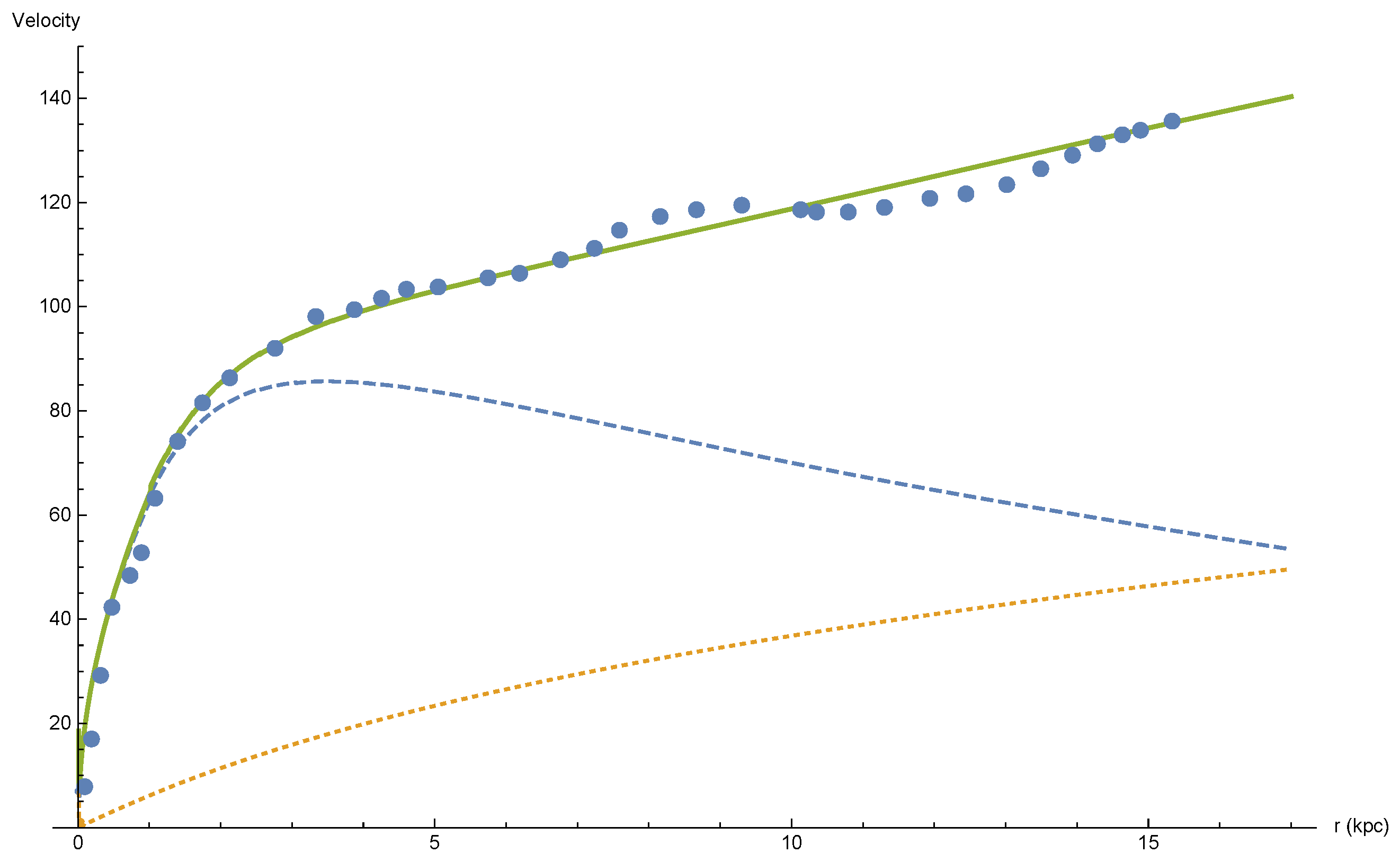
It is known that GR is verified by many types of observations. However, currently, the Newton–Einstein gravitational theory is at a crossroads. It has much in its favor observationally, and it has some very disquieting challenges. The successes that it has achieved in both astrophysical and cosmological scales have to be considered in light of the fact that GR needs to appeal to two unconfirmed ingredients, dark matter and energy, to achieve these successes. Dark matter has not only been with us since the 1920s (when it was initially known as the missing mass problem), but it has also become severe as more and more of it had to be introduced on larger distance scales as new data have become available. Moreover, 40-year-underground and accelerator searches and experiments have failed to establish its existence. The dark matter situation has become even more disturbing in recent years as the Large Hadron Collider was unable to find any super symmetric particle candidates, the community’s preferred form of dark matter. While things may still take a turn in favor of the dark matter hypothesis, the current situation is serious enough to consider the possibility that the popular paradigm might need to be amended in some way if not replaced altogether. In our recent work we have sought such a modification. Unlike other ideas such as Milgrom’s MOND [11], Mannheim’s Conformal Gravity [12,13,14], Moffat’s MOG [15] or theories and scalar-tensor gravity [16], the present approach is the minimalist one adhering to the razor of Occam. It suggests to replace dark matter by the retardation effect within standard GR. Fritz Zwicky noticed in 1933 that the velocities of Galaxies within the Comma Cluster are much higher than those predicted by the virial calculation that assumes Newtonian theory [17]. He calculated that the amount of matter required to account for the velocities could be 400 times greater with respect to that of visible matter, which led to suggesting dark matter throughout the cluster. In 1959, Volders, pointed out that stars in the outer rims of the nearby galaxy M33 do not move according to Newtonian theory [18]. The virial theorem coupled with Newtonian Gravity implies that , thus the expected rotation curve should at some point decrease as . During the 1970s, Rubin and Ford [19,20] showed that, for a large number of spiral galaxies, this behavior can be considered generic: velocities at the rim of the galaxies do not decrease—but they attain a plateau at some unique velocity, which differs for every galaxy. We have shown that such velocity curves can be deduced from GR if retardation is not neglected. The derivation of the retardation force is described in previous publications [21,22,23,24,25,26,27,28], see for example Figure 1. It should be noted that “dark matter” effects on light rays (gravitational lensing) are well handled when taking into account retardation [29].
The effects of gravitational lensing and the explanation of the anomalous perihelion advance of the planet Mercury were the first corroborated predictions of GR. Einstein made unpublished work on gravitational lensing as early as 1912 [30] (see Figure 2). As we mentioned previously in 1915 Einstein showed how GR explained the anomalous perihelion advance of the planet Mercury without any arbitrary parameters [31] (for a detailed account of Einstein’s previous unsuccessful attempts to obtain the same see Weinstein [32]), in 1919 an expedition led by Eddington confirmed GR’s prediction for the deflection of starlight by the Sun in the total Solar eclipse of 29 May 1919 [33,34], making Einstein instantly famous [31]. The reader should recall that there was a special significance to a British scientist confirming the prediction of a German scientist after the bloody battles of World War 1.
Figure 1.
Velocity curve for M33. Observational points were obtained by Dr. Michal Wagman, a former PhD student under my supervision, using Ref. [35]; the full line describes the rotation curve, which is the sum of the dotted line, describing the retardation contribution, and the dashed line, which is Newtonian.

Gravitational retardation effects do not seem to be very important in the Solar system, up to small corrections the dynamics is well described by Newtonian mechanics, and even the small GR effects observed can be well explained by a constant Schwarzschild metric, that is without time dependency effects of the metric. Still, it is perhaps too early to dismiss any time dependent effects on account of the discrepancy described in Table 1 with regard to the perihelion precession of Mercury, which is the reason for our study.
2. General Relativity
The general theory of relativity is based on two fundamental equations, the first being Einstein equations [36,37,38,39]:
where stands for the Einstein tensor (see Equation (8)), indicates the stress–energy tensor (see Equation (4)), (Greek letters are indices in the range 0–3). The second fundamental equation that GR is based on is the geodesic equation:
are the coordinates of the particle in spacetime, p is a typical parameter along the trajectory that for massive particles is chosen to be the length of the trajectory (), or the proper time () is the -th component of the 4-velocity of a massive particle moving along the geodesic trajectory (increment of x per p) and is the affine connection (Einstein summation convention is assumed). The stress–energy tensor of matter is usually taken in the form:
In the above, is the pressure and is the mass density. We remind the reader that lowering and raising indices is done through the metric and inverse metric , such that . The same metric serves to calculate s:
The affine connection is connected to the metric as follows:
Using the affine connection we calculate the Riemann and Ricci tensors and the curvature scalar:
which, in turn, serves to calculate the Einstein tensor:
Hence, the given matter distribution determines the metric through Equation (2) and the metric determines the geodesic trajectories through Equation (3).
3. Linear Approximation of GR—Justification
Only in extreme cases of compact objects (black holes and neutron stars) and the primordial reality or the very early universe does one need to not consider the solution of the full non-linear Einstein Equation [21]. In typical cases of astronomical interest (private communication with the late Professor Donald Lynden-Bell), certainly everywhere in the Solar system, one can use a linear approximation to those equations around the flat Lorentz metric such that:
In order to appreciate the above statements, let us look at the Schwarzschild metric [38]. This metric describes a static spherically symmetric mass distribution and is thus less general than the approach we intend to develop in this paper. It does have one advantage, however, and this is the ability to take into account strong gravitational fields and not just weak ones. This advantage is irrelevant in most astronomical cases in which gravity is weak and must only be considered for trajectories near compact objects (black holes and neutron stars). Here we introduce it just for the sake of making an order of magnitude estimate. The Schwarzschild squared interval can be written as:
In which are spherical coordinates and the point massive body is located at . The Schwarzschild radius is defined as:
in which M is the mass of the point particle. The most massive object in the Solar system is the Sun with a Solar mass of leading to . The deviation of the metric from the empty space Minkowski metric according to Equation (11) is:
Here is strongest on the Sun’s surface where in which , this is quite small (with respect to unity) indeed. For Mercury the closer distance to the Sun (perihelion) is hence at most. Neglecting the second order terms thus means neglecting terms of order and seems quite justified.
4. Linear Approximation of GR—The Metric
One then defines the quantity:
for non diagonal terms. For diagonal terms:
It can be shown ([36] page 75, Exercise 37, see also Refs. [37,38,39]) that one can choose a gauge such that the Einstein equations are:
Equation (16) can always be integrated to take the form [40]:
For reasons why the symmetry between space and time is broken, see Refs. [41,42]. The factor before the integral is small: in MKS units; hence, in the above calculation one can take , which is zero order in . In the zeroth order:
And also:
Assuming the reasonable assumption that the said massive body is composed of particles of non relativistic velocities:
and also:
Let us now look at Equation (4). We assume and, taking into account Equation (20), we arrive at , while other tensor components are significantly smaller. Thus, is significantly larger than other components of which are ignored from now on. One should notice that it is possible to deduce from the gauge condition in Equation (16) the relative order of magnitude of the relative components of :
Thus, the zeroth derivative of (which contains a as ) is the same order as the spatial derivative of meaning that is of order smaller than . The zeroth derivative of (which appears in Equation (22)) is the same order as the spatial derivative of . Meaning that is of order with respect to and of order with respect to .
In the current approximation, the following results hold:
(The underline signifies that the Einstein summation convention is not assumed).
We can summarize the above results in a concise formula:
in which is Kronecker’s delta. Thus:
and the proper time is:
for slow particles this reduces to:
and thus:
The above somewhat complex relation is the main reason that we will prefer to perform our analysis with rather than keeping in mind that in the Solar system for slow moving bodies (with respect to the speed of light).
It will be useful to introduce the gravitational potential which is defined below and can be calculated using Equation (17):
from the above definition and Equation (24) it follows that:
Let us now calculate the affine connection in the linear approximation:
taking into account Equation (27) we arrive at the result:
the above equation is only correct for a Latin index a; this is our main concern, as we will concentrate on the analysis of (rather than ).
5. Linear Approximation of GR—The Trajectory
Let us start by calculating the trajectory by inserting Equation (35) into Equation (3), we arrive at the equation:
We may write:
Thus:
As the current analysis is only valid for the first order in and since the right hand side of the equation is already linear in we only need to consider the other expressions on the right-hand side to zeroth order in , thus:
It follows that according to Equation (5):
and also:
Thus we obtain:
or in vector form:
In term of the potential this takes the form:
If the body is slow moving such that it follows that , , and thus:
if does not depend explicitly on time: and we obtain:
thus we are back to the Newtonian equation of motion, which can be used as a good approximation for most purposes to derive planetary motion.
5.1. “Angular Momentum”
Let us perform a vector multiplication of Equation (43) with the vector . We obtain:
Now suppose that in which , in this case . Thus:
the last equation sign is correct to the first order in (which is the order of our entire analysis). We now define an “angular momentum”:
in which m is the mass of the particle under consideration. The right-hand side of the equation is correct for slow bodies, in the Solar system. It follows that:
Hence for each Cartesian component:
Or also:
Thus:
in which is constant. This implies that the “angular momentum” has a size that depends on :
and a fixed direction:
We conveniently choose this direction to point in the z axis, hence:
Since the direction of is fixed and perpendicular to the direction of both and it follows that both vectors lie in the plane. Thus we can conveniently describe their motion using the standard polar coordinates . We underline that unlike the angular momentum vector of classical mechanics, this vector is only fixed in direction but not in size. We also underline that nowhere did we imply that the velocity of the particle must be small with respect to the velocity of light.
5.2. “Energy”
Let us make a scalar multiplication of Equation (43) with to obtain:
For a without explicit time dependence we have:
it follows that:
the term in parenthesis in the right-hand side needs only to be evaluated to zeroth order in and this can be done using Equation (40):
in which we use the definition for the potential given in Equation (33). Hence we obtain the conserved “energy”:
the “energy” is defined for either fast or slow bodies, while the right-hand ≃ relates only to slow bodies.
5.3. Polar Coordinates
By introducing polar coordinates we may write Equations (49) and (61) as follows:
the above forms seem quite classical, however, one should remember that the derivatives are with respect to the proper time of the body and not with respect to the global t coordinate. One should also recall that J is not constant and can vary to a small extent. Thus we eliminate and obtain:
The above result is quite classical except for the last term, which is a relativistic correction as is disclosed by the appearing there. To put the above result in a form that is closer to the forms that are found in the literature [9,39], we make the following observation. We have written as is usually done for spherical coordinates. However, notice that r in the above is not strictly a radial coordinate, which is defined as the circumference, divided by , of a sphere centered around the massive body. In fact, from Equation (28), it is clear that the appropriate radial coordinate is:
which is a small correction to r. Now, calculating the differential it follows that:
If we assume a Schwarzschild metric according to Equation (13):
where the last equality is correct to the first order. Alternatively one can use Equation (32) to calculate the gravitational potential for a static point mass to obtain:
and then plug this into Equation (33) to again obtain:
It now follows that:
Plugging Equation (69) into Equation (65) leads to:
Hence to first order in :
Using the results Equations (64) and (71) the interval given in Equation (28) can be rewritten as:
As to first order in :
and taking into account Equation (13), we obtain:
Thus the first order of our metric is identical to Schwarzschild’s for the case of a static point particle. This makes our analysis superior as it addresses the case of a general density distribution and does not ignore the possibility of time dependence.
In terms of we may write the energy as:
The relativistic correction has a dependence and the greater it is the closer the object is to the gravitating point mass, which represents the Sun. We also notice that in terms of one may write up to first order in :
which is reminiscent of the well known classical result regrading the conservation of angular momentum.
5.4. Integration of the Equations of Motion
Using Equation (76), we may write:
Defining (the symbol has nothing to do with the previously defined and is chosen this way in order to comply with the symbol used in the literature [9]):
Plugging Equation (78) into Equation (75) we arrive at the result:
Or:
Which is exactly the Padmanabhan [9] equation 7.114 (page 318), with a slightly different notation:
The analysis of Padmanabhan [9] of Equation (80) leads to Equation (1) and will not be repeated here due to lack of space. The interested reader is referred to the original text. We only mention that the semi-major axis, can be calculated by:
and the eccentricity can be calculated as:
Recently Křížek [43] has commented regarding the uncertainties related to the approximation needed in order to derive Equation (1) from Equation (80). The integration of Equation (80) involves elliptic functions, and the derivation of Equation (1) is not exact but involves approximations to those integrals, thus errors are introduced, which should be accounted for.
6. Metric Correction and the Gravitational Potential
So far we have considered only a naive model in which the Sun was taken to be a static point particle in the inertial frame, this has led us from Equation (67) to Equation (1). However, we can certainly do better, as it is well known that Equation (32) can be integrated for a particle p of mass moving in an arbitrary trajectory with velocity , resulting in a Liénard–Wiechert potential [40,44,45]:
The peculiar thing about this equation is that it must be evaluated at a retarded time , which is only given in terms of an implicit equation. This equation requires knowledge of the evaluation point of the potential and the knowledge of the particles trajectory for its solution, which is highly inconvenient. The derivative of the global time coordinate t with respect to the particular retardation time related to a certain particle is:
Which implies that for a slow moving particle with we arrive at the classical gravitational potential:
If many slow moving bodies affect a particular body, this body will move under the influence of a potential:
this is essentially Křížek’s [46] Equation (7) (given in terms of potential rather than force). In the Mercury case the most dominant body influencing its trajectory is the Sun, which is much more massive than the other planets in the Solar system, thus to a zeroth order approximation we can ignore the other planets altogether. However, for more subtle effects such as the precession of the perihelion for Mercury they cannot be ignored. Indeed, most of the precession can be attributed to the effect of the various planets as is indicated in the first row of Table 1 [7,8]. Křížek’s [46] has correctly criticized the lack of any error bar to this number, which must result from the uncertainty in the other planet masses and trajectories. This should be contrasted with the uncertainty attributed to the observed precession of the perihelion for Mercury in the same table.
As indicated, previously relativistic corrections in Equation (84) are only relevant for fast moving bodies with a considerable . The highest in the Solar system is for Mercury itself with × km/s yielding a × . However, the highest velocity among the other planets affecting Mercury’s orbit is Venus, with × km/s, yielding a × . Thus the relativistic corrections are small corrections to the contribution that the other planets make to the gravitational potential experienced by Mercury. These contributions are quite small even before a relativistic correction is applied. It thus remains to analyze the corrections to the gravitational potential of the Sun.
The Schwarzschild-based analysis, as well as the one presented in the previous sections assumes that the Sun is static and is located at the origin of axes. The Liénard-Wiechert potential described above allows us to take into account various corrections to the above simplified assumptions. The Sun does not need to be located at the origin of axis, and it can be moving with respect to the inertial frame. The motion of the Sun as well as the time gravity propagates from the Sun to Mercury both affect the gravitational potential. All these effects are small but not necessarily of the same magnitude, hence we need to evaluate their relative strengths.
Classical mechanics teaches us that a frame in which the Sun is located at the origin of axis is not inertial. A classical system that is inertial is one in which the origin of the axis is located at the center of the mass. This is only true in classical mechanics, however, the relativistic engine effect described in Refs. [47,48,49,50,51,52,53] shows that the relativistic retardation phenomena may cause even the center of the mass to accelerate, and thus cannot be used in strictly fixing an inertial frame.
Nevertheless, we shall assume for now that the center of mass does define an inertial frame and discuss the effect of the motion of the Sun with respect to it. The velocity of the Sun from the center of mass is estimated to be m/s [54] yielding a × . The difference between the potential and the potential given in Equation (67) is defined as:
The difference can be written in terms of three terms:
Those terms can be approximated to the first order as follows:
It is apparent that and cancel each other to first order in as expected, while the second order corrections in are negligible. Thus we may write a more accurate potential due to the Sun as:
Taking into account the distance of the Sun from the barycenter (see Figure 3 of Křížek [46]) it follows that it is of the order of the Sun’s diameter, while the exact trajectory of the Sun with respect to the Solar system barycenter is quite complex. Thus:
The analytical approach described above is not useful for calculating the trajectory in the presence of the potential correction. The potential now depends on time and thus the energy is not strictly conserved, moreover the potential depends on the polar angle and thus angular momentum is not conserved in an exact sense. Thus it seems best to integrate the equations numerically, however, this is beyond the scope of the present paper. A crude model that can accommodate the present approach would be to replace the Sun’s mass with an effective mass:
Thus the anomalous perihelion shift is not the value given by Equation (1) but rather by:
for Mercury the semi-major axis is km and the eccentricity is thus:
Thus the calculated value can be easily put within the error bar of the observed value as we recall that the discrepancy is only about per century. Other uncertainties may arise regarding the Newtonian contributions of the other planets to the gravitational potential [46].
7. Conclusions
We have shown that one can solve the Mercury trajectory problem using the weak gravitational approximation to GR and without using the Schwarzschild metric. This is contrary to the claims that this problem can only be solved in the framework of strong gravity [9]. In fact, it can easily be seen that the weak gravity approximation will suffice anywhere in the Solar system, and Mercury is no exception to this rule.
We have presented a solution to the current discrepancy between the observed and calculated perihelion shift although the solution is crude and numerical simulations may reveal more details.
The weak field approximation accounts for retardation, however, the retardation correction is of order , as should be expected, and is thus unimportant in the Mercury trajectory problem, certainly compared to the corrections related to the motion of the center of the Sun with respect to the barycenter of the Solar system. In this respect the Mercury perihelion problem is quite different than the “dark matter” problem, although the weak gravity approach can handle them both.
Funding
This research received no external funding.
Institutional Review Board Statement
Not applicable.
Informed Consent Statement
Not applicable.
Data Availability Statement
Not applicable.
Conflicts of Interest
The author declares no conflict of interest.
References
- Le Verrier, U. Lettre de M. Le Verrier à M. Faye sur la théorie de Mercure et sur le mouvement du périhélie de cette planète. Comptes Rendus Hebd. Séances L’Académie Sci. 1859, 49, 379–383. (In France) [Google Scholar]
- Carter, W.E.; Carter, M.S. Simon Newcomb, America’s first great astronomer. Phys. Today 2009, 62, 46. [Google Scholar] [CrossRef]
- Levenson, T. The Hunt for Vulcan. And How Albert Einstein Destroyed a Planet, Discovered Relativity, and Deciphered the Universe; Random House Publishing Group: New York, NY, USA, 2015; p. 80. [Google Scholar]
- Baum, R.P.; Sheehan, W. In Search of Planet Vulcan: The Ghost in Newton’s Clockwork; Basic Books: New York, NY, USA, 2003. [Google Scholar]
- Albert, E. The Foundation of the General Theory of Relativity. Annalen der Physik. 1916, 49, 769–822. [Google Scholar]
- Albert, E. Näherungsweise Integration der Feldgleichungen der Gravitation. In Sitzungsberichte der Königlich Preussischen Akademie der Wissenschaften Berlin; Part 1; The Prusssian Academy of Sciences: Berlin, Germany, 1916; pp. 688–696. [Google Scholar]
- Clemence, G.M. The Relativity Effect in Planetary Motions. Rev. Mod. Phys. 1947, 19, 361–364. [Google Scholar] [CrossRef]
- Park, R.S.; Folkner, W.M.; Konopliv, A.S.; Williams, J.G.; Smith, D.E.; Zuber, M.T. Precession of Mercury’s Perihelion from Ranging to the MESSENGER Spacecraft. Astron. J. 2017, 153, 121. [Google Scholar] [CrossRef]
- Padmanabhan, T. Gravitation—Foundations and Frontiers; Cambridge University Press: Cambridge, UK, 2010. [Google Scholar]
- Biswas, A.; Mani, K.R. Relativistic perihelion precession of orbits of Venus and the Earth. Cent. Eur. J. Phys. 2008, 6, 754–758. [Google Scholar] [CrossRef] [Green Version]
- Milgrom, M. A modification of the Newtonian dynamics as a possible alternative to the hidden mass hypothesis. Astrophys. J. 1983, 270, 365–370. [Google Scholar] [CrossRef]
- Mannheim, P.D.; Kazanas, D. Exact vacuum solution to conformal Weyl gravity and galactic rotation curves. Astrophys. J. 1989, 342, 635. [Google Scholar] [CrossRef]
- Mannheim, P.D. Linear Potentials and Galactic Rotation Curves. Astrophys. J. 1993, 149, 150. [Google Scholar] [CrossRef]
- Mannheim, P.D. Are Galactic Rotation Curves Really Flat? Astrophys. J. 1997, 479, 659. [Google Scholar] [CrossRef] [Green Version]
- Moffat, J.W. Scalar-Tensor-Vector Gravity Theory. J. Cosmol. Astropart. Phys. 2006, 2006, 4. [Google Scholar] [CrossRef]
- Corda, C. Interferometric detection of gravitational waves: The definitive test for General Relativity. Int. J. Mod. Phys. D 2009, 18, 2275. [Google Scholar] [CrossRef]
- Zwicky, F. On a New Cluster of Nebulae in Pisces. Proc. Natl. Acad. Sci. USA 1937, 23, 251–256. [Google Scholar] [CrossRef] [Green Version]
- Volders, L.M.J.S. Neutral Hydrogen in M33 and M101. Bull. Astr. Inst. Netherl. 1959, 14, 323. [Google Scholar]
- Rubin, V.C.; Ford, W.K., Jr. Rotation of the Andromeda Nebula from a Spectroscopic Survey of Emission Regions. Astrophys. J. 1970, 159, 379. [Google Scholar] [CrossRef]
- Rubin, V.C.; Ford, W.K., Jr.; Thonnard, N. Rotational Properties of 21 Sc Galaxies with a Large Range of Luminosities and Radii from NGC 4605 (R = 4 kpc) to UGC 2885 (R = 122 kpc). Astrophys. J. 1980, 238, 471. [Google Scholar] [CrossRef]
- Yahalom, A. The effect of Retardation on Galactic Rotation Curves. J. Phys. Conf. Ser. 2019, 1239, 012006. [Google Scholar] [CrossRef]
- Yahalom, A. Retardation Effects in Electromagnetism and Gravitation. In Proceedings of the Material Technologies and Modeling the Tenth International Conference, Ariel University, Ariel, Israel, 20–24 August 2018. [Google Scholar]
- Yahalom, A. Dark Matter: Reality or a Relativistic Illusion? In Proceedings of the Eighteenth Israeli-Russian Bi-National Workshop 2019, The Optimization of Composition, Structure and Properties of Metals, Oxides, Composites, Nano and Amorphous Materials, Ein Bokek, Israel, 17–22 February 2019. [Google Scholar]
- Wagman, M. Retardation Theory in Galaxies. Ph.D. Thesis, Senate of Ariel University, Samria, Israel, 2019. [Google Scholar]
- Yahalom, A. Lorentz Symmetry Group, Retardation, Intergalactic Mass Depletion and Mechanisms Leading to Galactic Rotation Curves. Symmetry 2020, 12, 1693. [Google Scholar] [CrossRef]
- Yahalom, A. Effects of Higher Order Retarded Gravity. Universe 2021, 7, 207. [Google Scholar] [CrossRef]
- Yahalom, A. The Cosmological Decrease of Galactic Density and the Induced Retarded Gravity Effect on Rotation Curves. J. Phys. Conf. Ser. 2021, 1956, 012002. [Google Scholar] [CrossRef]
- Yahalom, A. Tully—Fisher Relations and Retardation Theory for Galaxies. Int. J. Mod. Phys. 2021, 30, 2142008. [Google Scholar] [CrossRef]
- Yahalom, A. Lensing Effects in Retarded Gravity. Symmetry 2021, 13, 1062. [Google Scholar] [CrossRef]
- Sauer, T. Nova Geminorum 1912 and the Origin of the Idea of Gravitational Lensing. Arch. Hist. Exact Sci. 2008, 62, 1–22. [Google Scholar] [CrossRef]
- Pais, A. Subtle is the Lord...: The Science and Life of Albert Einstein; Oxford University Press: Oxford, UK, 1982; ISBN 978-0-19-853907-0. [Google Scholar]
- Weinstein, G. Einstein and the problem of confirmation by previously known evidence: A comment on Michel Janssen and Jurgen Renns Einstein and the Perihelion Motion of Mercury. arXiv 2022, arXiv:2201.00807v1. [Google Scholar]
- Dyson, F.W.; Eddington, A.S.; Davidson, C.R. A Determination of the Deflection of Light by the Sun’s Gravitational Field, from Observations Made at the Solar eclipse of May 29, 1919. Phil. Trans. R. Soc. A. 1920, 220, 291–333. [Google Scholar] [CrossRef]
- Kennefick, D. Not Only Because of Theory: Dyson, Eddington and the Competing Myths of the 1919 Eclipse Expedition. In Proceedings of the 7th Conference on the History of General Relativity, Tenerife, Spain, 10–14 March 2005; Volume 0709, p. 685. [Google Scholar] [CrossRef]
- Corbelli, E. Dark matter and visible baryons in M33. Mon. Not. R. Astron. Soc. 2003, 342, 199–207. [Google Scholar] [CrossRef] [Green Version]
- Narlikar, J.V. Introduction to Cosmology, 2nd ed.; Cambridge University Press: Cambridge, UK, 1993. [Google Scholar]
- Eddington, A.S. The Mathematical Theory of Relativity; Cambridge University Press: Cambridge, UK, 1923. [Google Scholar]
- Weinberg, S. Gravitation and Cosmology: Principles and Applications of the General Theory of Relativity; John Wiley & Sons, Inc.: Hoboken, NJ, USA, 1972. [Google Scholar]
- Misner, C.W.; Thorne, K.S.; Wheeler, J.A. Gravitation; W.H. Freeman & Company: New York, NY, USA, 1973. [Google Scholar]
- Jackson, J.D. Classical Electrodynamics, 3rd ed.; Wiley: New York, NY, USA, 1999. [Google Scholar]
- Yahalom, A. The Geometrical Meaning of Time. Found. Phys. 2008, 38, 489–497. [Google Scholar] [CrossRef]
- Yahalom, A. The Gravitational Origin of the Distinction between Space and Time. Int. J. Mod. Phys. D 2009, 18, 2155–2158. [Google Scholar] [CrossRef]
- Křížek, M. Relativistic perihelion shift of Mercury revisited. Astron. Nachrichten 2022, 343, e2022001. [Google Scholar] [CrossRef]
- Liénard, A. Champ électrique et magnétique produit parune charge concentrée en un point et animée d’un mouvement quelconque. L’éclairage Electrique 1898, 16, 5. [Google Scholar]
- Wiechert, E. Elektrodynamische Elementargesetze. Annalen der Physik 1901, 309, 667–689. [Google Scholar] [CrossRef] [Green Version]
- Křížek, M. Influence of celestial parameters on Mercury’s perihelion shift. Bulg. Astron. J. 2017, 27, 41. [Google Scholar]
- Tuval, M.; Yahalom, A. Newton’s Third Law in the Framework of Special Relativity. Eur. Phys. J. Plus 2014, 129, 240. [Google Scholar] [CrossRef] [Green Version]
- Yahalom, A. Retardation in Special Relativity and the Design of a Relativistic Motor. Acta Phys. Pol. 2017, 131, 1285–1288. [Google Scholar] [CrossRef]
- Tuval, M.; Yahalom, A. Momentum Conservation in a Relativistic Engine. Eur. Phys. J. Plus 2016, 131, 374. [Google Scholar] [CrossRef]
- Yahalom, A. Preliminary Energy Considerations in a Relativistic Engine. In Proceedings of the Israeli-Russian Bi-National Workshop, The Optimization of Composition, Structure and Properties of Metals, Oxides, Composites, Nano—and Amorphous Materials, Ariel, Israel, 28–31 August 2017; pp. 203–213. [Google Scholar]
- Rajput, S.; Yahalom, A. Material Engineering and Design of a Relativistic Engine: How to Avoid Radiation Losses. In Advanced Engineering Forum; Trans Tech Publications Ltd.: Wollerau, Switzerland, 2020; Volume 36, pp. 126–131. [Google Scholar]
- Rajput, S.; Yahalom, A.; Qin, H. Lorentz Symmetry Group, Retardation and Energy Transformations in a Relativistic Engine. Symmetry 2021, 13, 420. [Google Scholar] [CrossRef]
- Rajput, S.; Yahalom, A. Newton’s Third Law in the Framework of Special Relativity for Charged Bodies. Symmetry 2021, 13, 1250. [Google Scholar] [CrossRef]
- Wright, J.T.; Kanodia, S. Barycentric Corrections for Precise Radial Velocity Measurements of Sunlight. Planet. Sci. J. 2020, 1, 38. [Google Scholar] [CrossRef]
Figure 2.
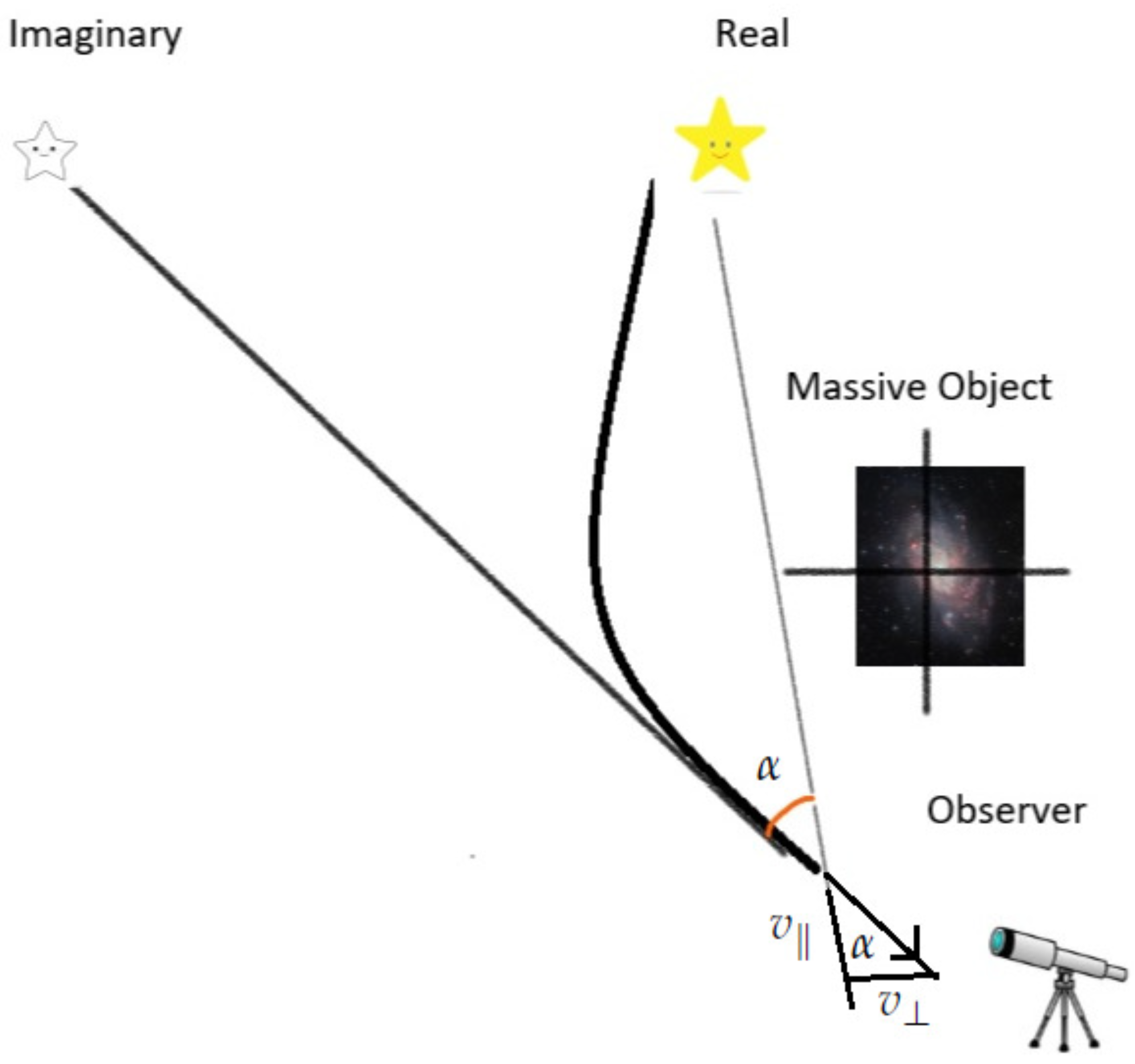
Light traveling toward the observer is bent due to the gravitational field of a massive object, thus a distant star appears to the observer at an angle with respect to its true location.
Figure 2.
Light traveling toward the observer is bent due to the gravitational field of a massive object, thus a distant star appears to the observer at an angle with respect to its true location.


Table 1.
The different contributions to the precession of perihelion for Mercury amount (arcsec/Julian century), theory vs. prediction.
Table 1.
The different contributions to the precession of perihelion for Mercury amount (arcsec/Julian century), theory vs. prediction.
| Causes of the Precession of Perihelion for Mercury (Arcsec/Julian Century) | Cause |
|---|---|
| 532.3035 | Gravitational tugs of other Solar bodies |
| 0.0286 | Oblateness of the Sun (quadruple moment) |
| 42.9799 | General Relativity effect (Schwarzschild—like) |
| −0.0020 | Lense-Thirring precession |
| 575.31 | Total predicted |
| 574.10 ± 0.65 | Observed |
Disclaimer/Publisher’s Note: The statements, opinions and data contained in all publications are solely those of the individual author(s) and contributor(s) and not of MDPI and/or the editor(s). MDPI and/or the editor(s) disclaim responsibility for any injury to people or property resulting from any ideas, methods, instructions or products referred to in the content. |
© 2022 by the author. Licensee MDPI, Basel, Switzerland. This article is an open access article distributed under the terms and conditions of the Creative Commons Attribution (CC BY) license (https://creativecommons.org/licenses/by/4.0/).
Share and Cite
MDPI and ACS Style
Yahalom, A. The Weak Field Approximation of General Relativity and the Problem of Precession of the Perihelion for Mercury. Symmetry 2023, 15, 39. https://doi.org/10.3390/sym15010039
AMA Style
Yahalom A. The Weak Field Approximation of General Relativity and the Problem of Precession of the Perihelion for Mercury. Symmetry. 2023; 15(1):39. https://doi.org/10.3390/sym15010039
Chicago/Turabian StyleYahalom, Asher. 2023. "The Weak Field Approximation of General Relativity and the Problem of Precession of the Perihelion for Mercury" Symmetry 15, no. 1: 39. https://doi.org/10.3390/sym15010039
Note that from the first issue of 2016, this journal uses article numbers instead of page numbers. See further details here.