
Solutions of 2-D Bratu Equations Using Lie Group Method
Department of Engineering Mathematics and Physics, Faculty of Engineering, Alexandria University, Alexandria 21544, Egypt
*
Author to whom correspondence should be addressed.
Symmetry 2022, 14(12), 2635; https://doi.org/10.3390/sym14122635
Submission received: 2 November 2022
/
Revised: 29 November 2022
/
Accepted: 2 December 2022
/
Published: 13 December 2022
(This article belongs to the Section Mathematics)
Abstract
:In this study, the nonlinear term in the two-dimensional Bratu equation has been replaced by its Taylor’s expansion. Hence, the resulting nonlinear partial differential equation has been studied using the Lie group method. The symmetry reductions that reduce nonlinear partial differential equations to ordinary differential equations are determined using the Lie group theory. The resultant ordinary differential equations were analytically solved, and the solutions were obtained in closed form for some specified parameter values, while others were solved numerically. We investigated the effect of increasing the value of the coefficient of the nonlinear term on the behavior of the solution in the obtained results, and the solutions were graphically presented.
1. Introduction
The evolution of nonlinear differential equations played an important role in many fields, such as fluid mechanics, chemical kinetics and plasma physics. Therefore, researchers are interested to obtain the exact solution of nonlinear differential equations. The Bratu equation appears in a large variety of applications, such as thermal reaction, radiative heat transfer, the fuel ignition model of thermal combustion, the Chandrasekhar model of the expansion of the universe, chemical reactor theory, non-deformable material of constant density during the ignition period and nanotechnology [1,2,3]. Recently, the Bratu equation was found in engineering, such as electro-spinning process for the manufacturing of nano-fibers. Nonlinear elliptic equations with boundary conditions of this type have been used to describe thermal explosions in the field of combustion theory (Gordon, Ko, & Shivaji, 2014) [4], as well as BVP emerging in the modelling of electrically conducting substances (Khuri & Wazwaz, 2013) [5].
In 1914, the Bratu equation was first set up by Bratu [6]. The generalization of the Bratu equation has been presented by Gelfand and Liouville. The equation is also used as a model for investigating the sun’s core temperature using the three-dimensional model Chandrasekhar (1967) [7]. In 1980, Adomian introduced and developed the Adomian decomposition method (ADM) [8]. The two-dimensional case was studied numerically by Boyd 1986 [9], Kapania (1990) [10], Misirli and Gurefe (2011) [11]. Bebernes and Eberly (1989) [12] used the Bratu equation with suitable boundary conditions to model the temperature distribution in combustion models. In 2018, Agheli introduced the approximation solution of Bratu differential equations using trigonometric basic functions [13]. He defined the values of the transformation in relation to trigonometric basis functions. The Bratu equation is widely used as a benchmarking tool for the validation of accuracy and effectiveness of numerical techniques. Bratu appears in several numerical methods, such as the finite difference method, finite element approximation, weighted residual method, a variational iteration scheme, Adomian decomposition method (ADM) (Wazwaz, 2005) [14] and homotopy analysis (Abbasbandy & Shivanian, 2010) [15].
Laplace transformed decomposition method (LTDM) (Khuri, 2004) [16], non-polynomial spline method (NSM) (Jalilian, 2010) [17], pseudo-spectral collocation method (Boyd, 2011) [18], Lie group shooting method (LGSM) (Abbasbandy, Hashemi, & Liu, 2011) [19] and nonlinear conjugate-gradient method (Mohsen, 2013) [20]. Stochastic solvers based on artificial intelligence using neural networks optimized and local research methodology are relatively less exploited in this domain. Artificial neural networks (ANNs) hybridized with the evolutionary approach are used to solve two-dimensional Bratu’s type equations (Raga, Ahmed, & Samar, 2013) [21]. Furthermore, this equation appears in a number of works that have been solved analytically and numerically [22,23,24].
The two-dimensional Bratu equation is given by
with the boundary conditions:
The exact solution to Equation (1) is given in [16] for can be positive and negative values, but we are interested in case is a positive value, in this case, is known as the Frank-Kamenetskii parameter in the combustion context.
Taylor’s expansion of the nonlinear term in (1) reads as
by substituting (3) in (1) we obtain
in this study, (4) will take two forms. The first called modified Bratu equation in linear form. Hence, (4) will be
the second is called modified Bratu equation in nonlinear form. Hence, (4) will be
Taylor’s expansion that is used in (1) enables us to obtain the linear form of Bratu (5) when we take the first and second term from (4). This is helpful, as polynomials are much easier to solve and deal with. If we use the number of terms of Taylor’s expansion, we obtain the nonlinear form of Bratu (6). As a result, we used the expansion to cope with the exponential part of Bratu (2).
The one-parameter group transformation is the mathematical technique used in this investigation. The Lie group method represents the group’s infinitesimals in terms of one or more functions known as infinitesimal functions, each of which is dependent on independent and dependent variables. The procedure for determining the infinitesimals is then reduced to determine the auxiliary equation, which can be obtained by solving a system of coupled linear partial differential equations known as the determining equations, which arise as a result of invoking the partial differential equations’ invariance and its auxiliary conditions.
We used the Lie group method to investigate the modified Bratu problem in this paper. The Lie group transformation methodology is an analytic technique. In the early nineteenth century, Norwegian mathematician Sophus Lie promoted this approach, which was later proposed by Ovsianikov and others [25,26,27]. The main idea of Lie symmetry analysis is to find continuous transformations with one or more parameters that keep the equation invariant [28,29,30,31]. The utility of the Lie point symmetry technique was widely demonstrated in a number of nonlinear differential equations encountered in various fields of applied research. Recently, the Lie group technique was used in a variety of works to solve linear and nonlinear problems, such as [32,33,34,35,36].
The above two cases (linear and nonlinear) have been considered. In the first case, we studied the modified Bratu equation in linear form, hence, we obtained two cases. In the first case, the analytical solution was in terms of Bessel function, while the analytical solution in the second case was in terms of trigonometric sine and cosine. Moreover, by solving the modified Bratu equation in nonlinear form, we also obtained two cases, the first case has been solved using Differential Transformation Method [37,38], while the second case has been solved numerically.
2. Lie Symmetry Group Method
Case (1): The modified Bratu equation in linear form
We consider the Bratu equation in the form.
according to Lie’s method, the infinitesimal generator [28,29,30,31] of the symmetry group is given by
in which are infinitesimal functions of the group variables. Then, the corresponding one-parameter Lie group of transformations is given by
if (9) is left invariant by the transformation then → . Equivalently, we can obtain by solving.
since (7) contains second derivative, so we evaluate the second prolongation.
where,
With . Therefore,
Solving the (13) we obtain the determining equations.
Solving (14), we obtain
the auxiliary equation will be
Sub case (1.1): By setting in (16) we obtain
Solving (17) we obtain
this type of symmetry converts the Bratu equation from rectangle geometry to cylindrical geometry.
By Substituting (18) in (7) we obtain
The general solution of (19) will be
where is called the Bessel function of the first kind of order , is called the Bessel function of the second of order , and , are arbitrary constants.
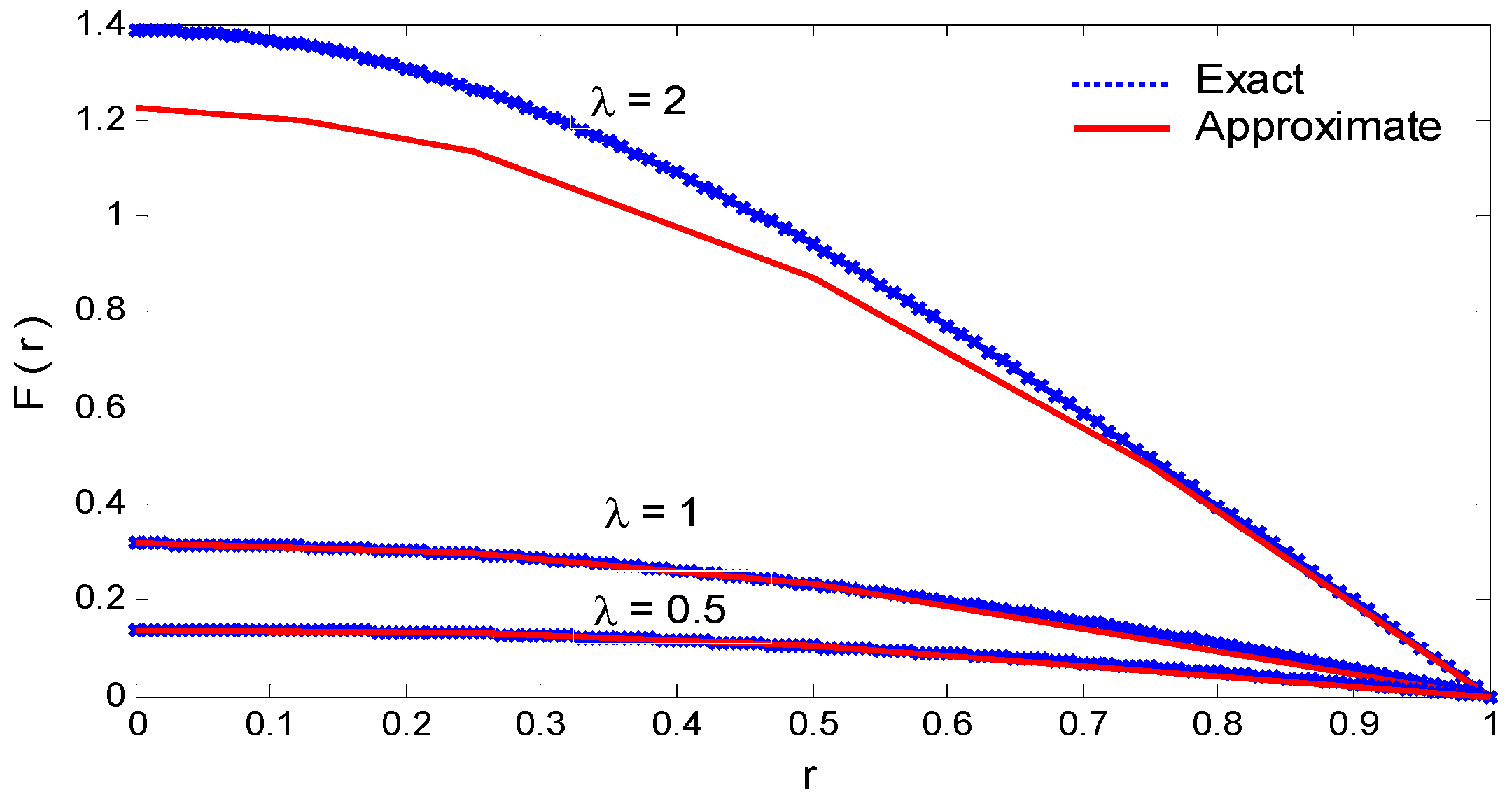
In Figure 1, we present the exact solution and the approximate analytical solution in (21) for in (22) for .
Since the two-dimensional Bratu equation is equivalent to the one-dimension boundary value problem given in [21]. Hence, by applying the boundary conditions (2) on (20) we obtain
Clearly, the solution of the modified Bratu equation in linear form is suitable only for . Moreover, it is evident that the values of increase when the parameter increases.
By substituting (21) in (18) we obtain
For , our result coincides with the result of [9].
Sub case (1.2): By setting in (16), we obtain.
Solving (23), we obtain.
by substituting (24) in (7) we obtain
Solution of (25) subject to boundary conditions in (2) will be
The solution in this case depends on two parameters; and . We compared our result with the exact solution in [21], by considering , therefore, . Hence, for and we found that the corresponding values of are , and , respectively.
In Figure 3, we present the exact and the approximate analytical solution in (26) for .
From Figure 3, by increasing the coefficient of nonlinear term in the modified Bratu equation , the error increased slightly. For this reason, one may use this approximate analytical form to describe the behavior of the solution. Moreover, we noticed that the values of increase when the parameter increases.
By substituting (26) in (24)
In Figure 4, we present travelling wave solution in (27) for and .
Case (2): The modified Bratu equation in nonlinear form
Considering Bratu’s equation in the form.
Repeating the same procedures as we did from (8) to (15), we obtain
the auxiliary equation will be
Sub Case (2.1): By setting in (30) we obtain
Solving (31), we obtain
by substituting (32) in (28), we obtain
To solve Equation (33) we used Differential Transformation Method.
Differential Transformation Method is a different approach to getting an analytic Taylor series solution to differential equations. The fundamental advantage of this method is that it may be immediately used in nonlinear equations without the need for linearization or discretization [37,38]. The concept of DTM was first introduced by Zhou [38] who solved linear and nonlinear problems in electrical circuits.
The differential transform of a function is defined as follows [37,38]:
and the inverse differential transform of is defined as:
In Table 1 we summarized the main theorems of the differential transform.
By multiplying (32) with , we obtain
From (36) and the main theorems in Table 1, we obtain
But
By the same method, we can obtain the other terms and .
Applying DTM on (36) and substituting it with (36a)–(36c) and the other terms that were mentioned above, we obtain
such that satisfies the relation
Equation (38) represents the transformation of (36) after applying the differential transformation method.
By setting , hence, by applying the differential transform method on (2), therefore, and . We summarized the relation between and in Table 2.
For the convergence of the power series, we require . The relation between and satisfy the equation .
Table 3 shows that the absolute error when is less than , while when is less than and finally when is less than . Hence, it is evident that the values of the absolute error increase when the parameter increases.
In Figure 5, we present the exact and the analytical approximate solutions in (39) for .
In this case, we found perfect match of our approximate solution with the exact solution for all values of .
By substituting (39) with (32), we obtain
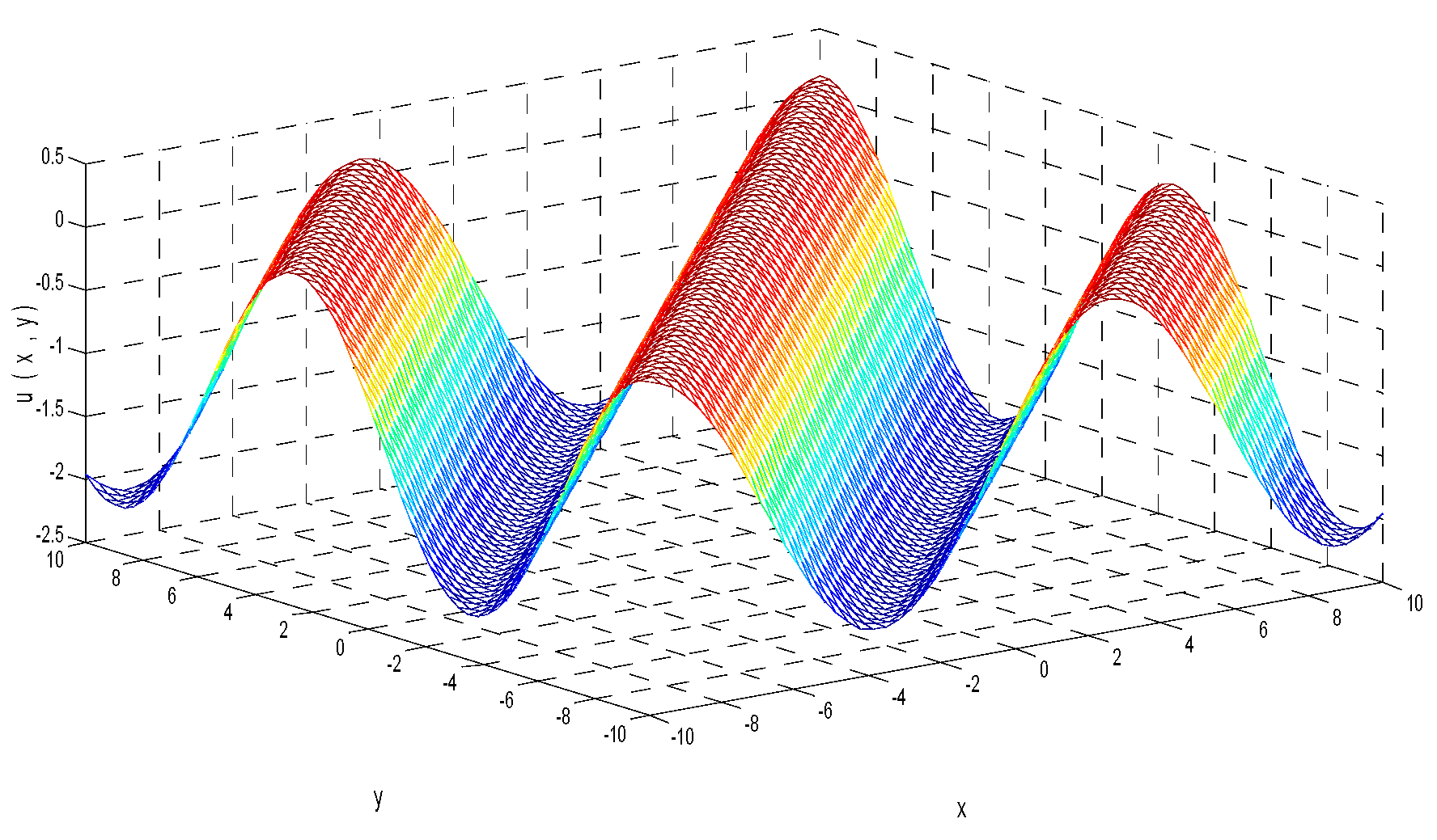
Figure 6 illustrate the behavior of the function u(x, y) that depends on the location of (x) and the location of (y).
Sub Case (2.2): By setting in (30) we obtain
By solving (41), we obtain
by substituting (42) with (27), we obtain
The numerical solution of (43) has been obtained for using fourth and fifth order Runge Kutta method. The values of the parameter in (43) have been chosen to adjust the value of to be close to the exact value in [6,9,21].
In Figure 7, we present exact solution and numerical solution in (43) for and the corresponding value of the parameter are , , respectively.
The numerical solution in this case is asymmetric about the origin point. Moreover, in the case of we could not find a value for so that the numerical solution matches the analytical solution at the origin point.
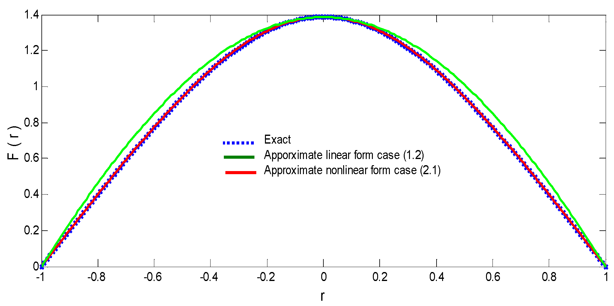
In Figure 8, we present exact solution and our approximate analytical solutions in (26) and (39) for .
Form Figure 8. Clearly, the exact solution and our approximate solutions of Bratu equations are symmetric about the origin. By comparing our approximate analytical solutions with the analytical solution in [25], we noticed that the cylindrical invariant solution of the modified Bratu equation in nonlinear form perfectly matches the exact solution.
3. Conclusions
The nonlinear Bratu equation has been solved using the Lie group approach, demonstrating the method’s efficiency in producing invariant solutions for partial differential equations with two independent variables. The approach reduces the nonlinear ordinary differential equation to the partial differential equation. The Lie group method proved that the modified Bratu equations in linear and nonlinear forms have two types of invariant solutions; the cylindrical solution and the travelling wave solution. It is evident that the values of and the absolute error increase when the parameter increases in all cases studied.
In the modified Bratu equation in linear form, the cylindrical solution was obtained in terms of Bessel function and depends on the value of , while the travelling wave solution was found in terms of cosine function and depends on and . The cylindrical solution of the modified Bratu equation in nonlinear form was obtained in series form using the differential transform method and depends on . It is evident that we obtained the best results with the series solution of the modified Bratu equation in nonlinear from for all values of , while all obtained solutions could be used only in case of between 0 and 1.
Author Contributions
M.B.A.-e.-M. was responsible for suggesting the problem, reviewing the results and editing the writing; A.M.A. validate the calculations and check the accuracy of plotted results, M.E.M. was responsible for the calculations and writing the manuscript. All authors have read and agreed to the published version of the manuscript.
Funding
The research received no external funding.
Data Availability Statement
Not applicable.
Acknowledgments
The authors like to express their gratitude and thanks to the potential reviewers for their critical review of the paper and for their valuable comments and suggestions that improved the paper to the present form.
Conflicts of Interest
The authors declare no conflict of interest.
References
- Gelfand, I.M. Some problems in the theory of quasi-linear equations. Usp. Mat. Nauk 1959, 14, 87–158. [Google Scholar]
- Wan, Y.Q.; Guo, Q.; Pan, N. Thermo-electro-hydrodynamic model for electro spinning process. Int. J. Nonlinear Sci. Numer. Simul. 2004, 5, 5–8. [Google Scholar] [CrossRef]
- Jacobsen, J.; Schmitt, K. The Liouville-Bratu-Gelfand problem for radial operators. J. Differ. Equ. 2002, 184, 283–289. [Google Scholar] [CrossRef] [Green Version]
- Gordon, P.V.; Ko, E.; Shivaji, R. Multiplicity and uniqueness of positive solutions for elliptic equations with nonlinear boundary conditions arising in a theory of thermal explosion. Nonlinear Anal. Real World Appl. 2014, 15, 51–57. [Google Scholar] [CrossRef]
- Khuri, S.A.; Wazwaz, A.M. A variational approach to a BVP arising in the modelling of electrically conducting solids. Cent. Eur. J. Eng. 2013, 3, 106–112. [Google Scholar] [CrossRef] [Green Version]
- Bratu, G. Sur les equations integrals non-lineaires. Bull. Soc. Math. France 1914, 42, 113–142. [Google Scholar] [CrossRef] [Green Version]
- Chandrasekhar, S. An Introduction to the Study of Stellar Structure; Dover Publications Inc.: New York, NY, USA, 1967. [Google Scholar]
- Adomian, G.A. Review of the Decomposition Method in Applied Mathematics. J. Math. Anal. Appl. 1988, 135, 501–544. [Google Scholar] [CrossRef] [Green Version]
- Boyd, J.P. An analytical and numerical study of the two-dimensional Bratu equation. J. Sci. Comput. 1986, 1, 183–206. [Google Scholar] [CrossRef] [Green Version]
- Kapania, R.K. A pseudo-spectral solution of 2-parameter Bratu equation. Comput. Mech. 1990, 6, 55–63. [Google Scholar] [CrossRef]
- Misirli, E.; Gurefe, Y. Exp-function method for solving nonlinear evolution equations. Math. Comput. Appl. 2011, 16, 258–266. [Google Scholar] [CrossRef] [Green Version]
- Bebernes, J.; Eberly, D. Mathematical Problems from Combustion Theory; Springer: New York, NY, USA, 1989; pp. 6–8. [Google Scholar]
- Agheli, B. Approximate solution of Bratu differential equation using trigonometric basic functions. Kragujev. J. Math. 2021, 45, 203–214. [Google Scholar] [CrossRef]
- Wazwaz, A.M. Adomian decomposition method for a reliable treatment of the Bratu-type equations. Appl. Math. Comput. 2005, 166, 652–663. [Google Scholar] [CrossRef]
- Abbasbandy, S.; Shivanian, E. Prediction of multiplicity of solutions of nonlinear boundary value problems: Novel application of homotopy analysis method. Commun. Nonlinear Sci. Numer. Simul. 2010, 15, 3830–3846. [Google Scholar] [CrossRef]
- Khuri, S.A. A new approach to Bratu’s problem. Appl. Math. Comput. 2004, 147, 131–136. [Google Scholar] [CrossRef]
- Jalilian, R. Non-polynomial spline method for solving Bratu’s problem. Comput. Phys. Commun. 2010, 181, 1868–1872. [Google Scholar] [CrossRef]
- Boyd, J.P. One-point pseudo spectral collocation for one-dimensional Bratu equation. Appl. Math. Comput. 2011, 217, 5553–5565. [Google Scholar] [CrossRef]
- Abbasbandy, S.; Hashemi, M.S.; Liu, C.S. The Lie group shooting method for solving the Bratu equation. Commun. Nonlinear Sci. Numer. Simul. 2011, 16, 4238–4249. [Google Scholar] [CrossRef]
- Mohsen, A. On the integral solution of the one-dimensional Bratu problem. J. Comput. Appl. Math. 2013, 251, 61–66. [Google Scholar] [CrossRef]
- Raja MA, Z.; Ahmed, S.I.; Samar, R. Neural network optimized with computing technique for solving the 2-dimensional Bratu problem. Neural Comput. Appl. 2013, 23, 2199–2210. [Google Scholar] [CrossRef]
- Buckmire, R. Application of a Mickens Finite-Difference Scheme to the Cylindrical Bratu–Gelfand Problem. Numer. Methods Partial. Differ. Equ. 2004, 20, 327–337. [Google Scholar] [CrossRef]
- Zis¸, T.O.; Yildirim, A. Comparison between adomian’s method and He’s homotopy perturbation method. Comput. Math. Appl. 2008, 56, 1216–1224. [Google Scholar]
- Aregbesola, Y.A.S. Numerical solution of Bratu problem using the method of weighted residual. Electron. J. S. Afr. Math. Sci. Assoc. 2003, 3, 1–7. [Google Scholar]
- Olver, P.J. Application of Lie Group to Differential Equations; Springer: Berlin/Heidelberg, Germany, 1986. [Google Scholar]
- Ovsiannikov, L.V. Group Analysis of Differential Equations; Academic Press: Cambridge, MA, USA, 1982. [Google Scholar]
- Hydon, P.E. Symmetry Methods for Differential Equations; Cambridge University Press: Cambridge, UK, 2000. [Google Scholar]
- Bluman, G.B.; Kumei, S. Symmetries and Differential Equation; Springer: Berlin/Heidelberg, Germany, 1989. [Google Scholar]
- Ibragimove, N.H. Handbook of Lie Group Analysis of Differential Equations; CRC Press: Boca Raton, FL, USA, 1994; Volume 1. [Google Scholar]
- Hill, J.M. Differential Equations and Group Methods for Scientists and Engineers; CRC Press: Boca Raton, FL, USA, 1992. [Google Scholar]
- Bluman, G.W.; Cheviakov, A.F.; Anco, S.C. Applications of Symmetry Methods to Partial Differential Equations; Springer: New York, NY, USA, 2010. [Google Scholar]
- Naderifard AHejazi, S.R.; Dastranj, E. Symmetry properties, conservation law and exact solutions of time- fractional irrigation equation. Waves Random Complex Media 2019, 29, 178–194. [Google Scholar] [CrossRef]
- Rashidi, S.; Hejazi, S. Lie symmetry approach for The Vlasov-Maxwell system of equations. J. Geom. Phys. 2018, 132, 1–12. [Google Scholar] [CrossRef]
- Rashidi, S.; Hejazi, S.; Mohammadizadeh, F. Group formalism of Lie transformations, conversation laws, exact and numerical solutions of nonlinear time-fractional Black-Scholes equation. J. Comput. Appl. Math. 2022, 403, 113863. [Google Scholar] [CrossRef]
- Hejazi, S.; Saberi, E.; Mohammadizadeh, F. Anisotropic nonlinear time-fractional diffusion equation with a source term: Classification via Lie point symmetries, analytic solutions and numerical solution. Appl. Math. Comput. 2021, 391, 125652. [Google Scholar] [CrossRef]
- Hejazi, S.; Naderifard, A. Dym equation: Group analysis and conservation laws. AUT J. Math. Comput. 2022, 3, 17–26. [Google Scholar]
- Hatami, M.; Ganiji, D.D.; Sheikholeslami, M. Differential Transformation Method for Mechanical Engineering Problems; Academic Press: Cambridge, MA, USA, 2016. [Google Scholar]
- Zhou, J.K. Differential Transformation and Its Applications for Electrical Circuits; Huazhong University Press: Wuhan, China, 1986. [Google Scholar]
Figure 1.
Represents the exact solution and the approximate analytical solution in (21) for in (22) for .
Figure 1.
Represents the exact solution and the approximate analytical solution in (21) for in (22) for .

Figure 2.
Represents u(x, y) in (22) for .

Figure 3.
Represents the exact and the approximate analytical solution in (26) for .

Figure 4.
Represents the travelling wave solution in (27) for and c = 1.0055.

Figure 5.
Represents the exact and the analytical approximate solutions in (39) for .

Figure 6.
Represents in (40) for .

Figure 7.
Represents exact solution and numerical solution in (43) for and the corresponding value of the parameter are , , respectively.
Figure 7.
Represents exact solution and numerical solution in (43) for and the corresponding value of the parameter are , , respectively.

Figure 8.
Represents exact solution and our approximate analytical solutions in (26) and (39) for .


Table 1.
The main theorems of the differential transform method.
| No | Original Function | Transformed Function |
|---|---|---|
| 1 | ||
| 2 | ||
| 3 | ||
| 4 | ||
| 5 |
Table 2.
Represents the relation between and f(k).
| 1 | |
| 2 | f(3) = 0 |
| 3 | |
| 4 | f(5) = 0 |
| 5 | |
| 6 | f(7) = 0 |
| 7 |
Table 3.
Represents the absolute error between the exact solution and our approximate solution.
Publisher’s Note: MDPI stays neutral with regard to jurisdictional claims in published maps and institutional affiliations. |
© 2022 by the authors. Licensee MDPI, Basel, Switzerland. This article is an open access article distributed under the terms and conditions of the Creative Commons Attribution (CC BY) license (https://creativecommons.org/licenses/by/4.0/).
Share and Cite
MDPI and ACS Style
Abd-el-Malek, M.B.; Amin, A.M.; Mahmoud, M.E. Solutions of 2-D Bratu Equations Using Lie Group Method. Symmetry 2022, 14, 2635. https://doi.org/10.3390/sym14122635
AMA Style
Abd-el-Malek MB, Amin AM, Mahmoud ME. Solutions of 2-D Bratu Equations Using Lie Group Method. Symmetry. 2022; 14(12):2635. https://doi.org/10.3390/sym14122635
Chicago/Turabian StyleAbd-el-Malek, Mina B., Amr M. Amin, and Mahmoud E. Mahmoud. 2022. "Solutions of 2-D Bratu Equations Using Lie Group Method" Symmetry 14, no. 12: 2635. https://doi.org/10.3390/sym14122635
Note that from the first issue of 2016, this journal uses article numbers instead of page numbers. See further details here.